Multiband imaging of the HD 36546 debris disk: a refined view from SCExAO/CHARISBased on data collected at Subaru Telescope, which is operated by the National Astronomical Observatory of Japan.Journal: AJ
Abstract
We present the first multi-wavelength (near-infrared; ) imaging of HD 36546’s debris disk, using the Subaru Coronagraphic Extreme Adaptive Optics (SCExAO) system coupled with the Coronagraphic High Angular Resolution Imaging Spectrograph (CHARIS). As a 3-10 Myr old star, HD 36546 presents a rare opportunity to study a debris disk at very early stages. SCExAO/CHARIS imagery resolves the disk over angular separations of (projected separations of ) and enables the first spectrophotometric analysis of the disk. The disk’s brightness appears symmetric between its eastern and western extents and it exhibits slightly blue near-infrared colors on average (e.g. JK) – suggesting copious sub-micron sized or highly porous grains. Through detailed modeling adopting a Hong scattering phase function (SPF), instead of the more common Henyey-Greenstein function, and using the differential evolution optimization algorithm, we provide an updated schematic of HD 36546’s disk. The disk has a shallow radial dust density profile ( and ), a fiducial radius of au, an inclination of , and a position angle of PA . Through spine tracing, we find a spine that is consistent with our modeling, but also with a “swept-back wing” geometry. Finally, we provide constraints on companions, including limiting a companion responsible for a marginal Hipparcos–Gaia acceleration to a projected separation of and to a minimum mass of .
I Introduction
Gas depleted, dust-dominated debris disks are critical targets for understanding the composition, structure, and (typically late-stage) formation of planetary systems (Wyatt 2008; Kenyon & Bromley 2008; Hughes et al. 2018). Scattered-light imaging of debris disks can reveal and characterize signatures of planets responsible for shaping the disks’ morphologies and help constrain the properties of the planets themselves (Kalas et al. 2005; Lagrange et al. 2010, e.g.). “Extreme adaptive-optics” (exAO) facilities, such as SPHERE (Beuzit et al. 2019), GPI (Macintosh et al. 2015), and SCExAO (Jovanovic et al. 2015; Lozi et al. 2018; Currie et al. 2020a), now deliver high-fidelity images of numerous debris disks at sub-arcsecond separations (Milli et al. 2017; Duchêne et al. 2020; Esposito et al. 2020; Lawson et al. 2020, e.g.).
Modeling of multi-wavelength imaging can enable analysis of the properties and composition of the constituent dust (Boccaletti et al. 2003; Fitzgerald et al. 2007; Goebel et al. 2018; Lawson et al. 2020, e.g.), providing a context for the chemistry and evolution of our own Kuiper belt (Currie et al. 2015b; Milli et al. 2017; Chen et al. 2020). However, the assumed scattering phase function (SPF) critically affects resulting model disk images and thus our ability to infer disk properties. The traditionally adopted Henyey-Greenstein (H-G) SPF (Henyey & Greenstein 1941) can reproduce scattered light images at large scattering angles but is not physically motivated and is often inconsistent with data at smaller scattering angles (Hughes et al. 2018, e.g.). Combined with evidence suggesting that the best-fit H-G SPF from disk modeling is correlated with the scattering angles probed by the data (rather than any more meaningful physical properties of the system), Hughes et al. 2018 suggest that some other SPF – capable of explaining debris disk imagery irrespective of the scattering angles probed – is needed. Lawson et al. 2020 showed that the Hong 1985 SPF, which is derived from observations of solar system zodiacal dust, reasonably reproduced near-infrared (NIR) imagery of the debris disk of HD 15115. This finding is consistent with the suggestion in Hughes et al. 2018 that a near-universal SPF may exist to explain observed scattered light of a particular wavelength originating from nearly any circumstellar dust. Moreover, Lawson et al. 2020 found that the adopted SPF can fundamentally change the interpretation of scattered light images, e.g. the number of separate dust populations required to reproduce the data. If scattered light imagery of additional systems can be well-modeled using this SPF, it could provide further evidence of such a universal SPF.
In this study, we present the first multi-wavelength scattered light imaging of the debris disk around HD 36546 (Currie et al. 2017), using the Subaru Coronagraphic Extreme Adaptive Optics (SCExAO) system and the Coronagraphic High Angular Resolution Imaging Spectrograph (CHARIS) integral field spectrograph in broadband (spanning NIR , , and bands, ) mode (Groff et al. 2016). HD 36546’s disk is highly inclined, bright in scattered light, and has an extremely high fractional luminosity ( 410-3) comparable to long-studied debris disks around Pictoris and HR 4796A and new benchmarks such as HD 115600 (Smith & Terrile 1984; Schneider et al. 2014; Currie et al. 2015b; Millar-Blanchaer et al. 2015; Gibbs et al. 2019).
The HD 36546 system lies at a distance of pc (Gaia Collaboration et al. 2018), slightly foreground to the Taurus-Auriga star-forming region and is a member of the 3–10 Myr old 118 Tau association (99.1% probability, Gagné et al. 2018)11 1 This association is labeled as “Mamajek 17” in Currie et al. 2017.. Due to the system’s extreme youth, the HD 36546’s debris disk represents a rare opportunity to study debris disk structure and composition at very early stages where protoplanetary disk accretion ceases, colder gas dissipates, and collisions between icy planetesimals tracing Kuiper belt-analogue formation are predicted to yield detectable debris at peak luminosity (Currie et al. 2008; Currie et al. 2009; Cloutier et al. 2014; Ribas et al. 2015; Kenyon & Bromley 2008).
Previous work on HD 36546 found evidence for a disk with an extremely large scale height and strong forward-scattering: an H-G value of 0.7–0.85, among the highest of any known debris disk (Currie et al. 2017; Hughes et al. 2018). Revisiting HD 36546’s disk with our new, comparable-quality data obtained over a wider wavelength range will provide improved constraints on its structure and the first look at its composition. Much like for the case with HD 15115 (Lawson et al. 2020), modeling these data with a different SPF may lead to revisions in our understanding of the HD 36546 disk’s properties.
Our new data resolve the disk down to separations as small as ( au) and enable the first spectrophotometric analysis of the disk. From these data, we provide surface brightness, surface contrast, and asymmetry profiles in CHARIS broadband and , , and bands – as well as disk color profiles in and . Through detailed forward modeling, we provide a refined schematic for HD 36546’s disk. Finally, we provide constraints for the presence of companions within the CHARIS field of view (FOV; angular separations of ).
II Data
II.1 Observations
We observed HD 36546 (Currie et al. 2017; Lisse et al. 2017, A0–A2V, V=6.95, H=6.92;) on 2019 January 12 using the Subaru Telescope’s SCExAO running at 2 kHz paired with the CHARIS integral field spectrograph (Groff et al. 2016) operating in low-resolution (R ), broadband (1.16–2.37 ) mode, and utilizing SCExAO’s Lyot coronagraph with 217 mas diameter occulting spot. Conditions were photometric with good 04–05 seeing and 16 km/hour winds22 2 However, AO performance was compromised compared to typical performance due to a significant (4–5x) loss in the IR secondary mirror’s reflectivity at blue optical wavelengths where AO188 (which provides a needed low-order correction for SCExAO) does wavefront sensing. This loss resulted from oxidization of the mirror’s silver coating from sulfur dioxide stemming from the Kilauea eruption in May 2018. For wavefront sensing, HD 36546 was effectively a magnitude 10.5 star. The mirrors were realuminized with a fresh coating in late 2019.. The data were collected in angular differential imaging mode (ADI; Marois et al. 2006) and achieved total parallactic angle rotation of with total integration time of 50 minutes. The data set is made up of 66 individual exposures, with 65 having exposure times of 45.73 seconds and one having an exposure time of 30.98 seconds. Sky frames were also obtained following the science data to enable sky subtraction.
A second target, HR 2466 (A2V; V = 5.21, H = 5.07), was observed on the same night with the same instrument configuration to enable reference star differential imaging (RDI). These data include 143 individual exposures of 20.65 seconds each, for a total integration time of 49 minutes. For all reduction and analysis, we adopt the revised CHARIS pixel scale of 00162 and the North-up PA offset of 22 as reported in Currie et al. 2018.
II.2 CHARIS Data Reduction
CHARIS data cubes were extracted from raw CHARIS exposures using the CHARIS Data Reduction Pipeline (Brandt et al. 2017), using modifications to read noise suppression listed in Currie et al. 2020a. Extracted data take the form of image cubes with dimensions (i.e. pixel images for each of 22 wavelength channels). Subsequent basic image processing – e.g. sky subtraction, image registration, spectrophotometric calibration – was carried out as in Currie et al. 2011; Currie et al. 2018. Inspection of registered data cubes showed that the quality of the AO correction varied between exposures taken before (good), during (worst33 3 This is a result of HD 36546 transiting very near zenith from Subaru, making alt/az tracking through transit challenging.), and after (best) transit. Particularly low quality frames were identified by first measuring the peak-to-halo flux ratio of the satellite spots in each exposure44 4 The peak flux is defined as the flux within an aperture with a radius of one instrumental full-width at half-maximum (FWHM), centered on the satellite spot. The halo flux is the flux within an annulus centered on the satellite spot, with inner and outer radii of FWHM and FWHM respectively, where dr is the radial extent that results in an annulus enclosing the same area as the peak aperture.. These values were then averaged over the 4 satellite spots and 22 wavelength channels, and the median and median absolute deviation of the values across the full data sequence were computed. Any exposures falling more than 3 median absolute deviations below the median peak-to-halo ratio were removed. We removed three frames near transit which met this criteria.
PSF subtraction to recover HD 36546’s disk was performed using RDI with the Karhunen-Loève Image Projection (KLIP; Soummer et al. 2012) algorithm (RDI-KLIP), as well as ADI with both KLIP (ADI-KLIP) and the Adaptive, Locally Optimized Combination of Images (A-LOCI; Currie et al. 2012a; Currie et al. 2015a) algorithm (ADI-ALOCI) which is based on the LOCI algorithm (Lafrenière et al. 2007). To search for planets, we exploit both ADI and spectral differential imaging (Sparks & Ford 2002, SDI;) (Beuzit et al. 2019, see e.g.,), using a more aggressive implementation of A-LOCI (Currie et al. 2018; Currie et al. 2020a; Currie et al. 2020b; Lawson et al. 2020, as in e.g.,). Unlike prior implementations, we performed an ADI-based reduction on the post-SDI residuals instead of SDI on the post-ADI residuals. We found that for data sets with somewhat variable AO corrections leading to temporally decorrelated images, the former approach is slightly superior. The utilized algorithm parameters are provided in Table 1.
| Method | Param. Tuning | Radial Prof. Sub. | Algorithm Parameters | |||
|---|---|---|---|---|---|---|
| RDI-KLIP | disk | False | 15 | 70 | 55 | , , |
| ADI-KLIP | disk | True | 15 | 65 | 50 | , , |
| ADI-ALOCI | disk | True | 15 | 70 | 5 | , , , |
| SDI+ADI-ALOCI | planet | True | 5 | 70 | 2.5 | , , , |
Note. — Algorithm settings for PSF subtraction with each of the three techniques utilized. ‘Radial Profile Sub.’ indicates whether each reduction was carried out on radial profile subtracted data. and refer to the inner and outer radii of the subtraction region for each reduction (in pixels). indicates the radial width of individual subtraction annuli. ‘g’ refers to the aspect ratio of the optimization regions (which are annular subsections, defined in polar-coordinates by radial and azimuthal extents) with producing azimuthally elongated regions and producing radially elongated regions. ‘’ refers to the area of optimization regions in units of PSF cores. ‘’ indicates the minimum rotation gap in units of PSF FWHM (for both A-LOCI and KLIP). ‘’ gives the radial size of subtraction regions in units of pixels (for both A-LOCI and KLIP). ‘’ indicates the number of principal components utilized in construction of the model PSF. ‘’ is the number of subsections into which each KLIP optimization annulus was divided (with a value of 1 corresponding to full annuli). ‘SVD’ refers to the threshold for normalized singular values below which A-LOCI coefficients are truncated. For the ADI-ALOCI reduction, the algorithm is not restricted in the number of images that may be used in constructing the PSF model. For the SDI+ADI-ALOCI parameter tuning, we also employed a moving pixel mask over the subtraction zone (Marois et al. 2010; Currie et al. 2012a) and restricted the reference PSF construction for each target image to the 50 best-correlated frames (Currie et al. 2012b).
II.3 Results
In broadband (wavelength-collapsed) imagery, all three PSF-subtraction techniques result in clear detection of the bright side of HD 36546’s disk to separations as small as (Figures 1, 2). Each result also shows a partial, weak detection of the fainter side of the disk in the west, which is strongest in the ADI-ALOCI result, with signal-to-noise ratio per resolution element (SNRE) . As in the discovery imagery of the disk from SCExAO/HiCIAO (Currie et al. 2017), SCExAO/CHARIS imagery of HD 36546 reveals a highly inclined, significantly asymmetrically scattering disk. ADI-based reductions reveal no obvious evidence of ansae, indicative of gaps or a ring-like structure, within the field of view. The RDI-KLIP reduction, however, appears to show a change in the disk profile at , consistent with the fiducial radius of the best-fitting disk model identified in Currie et al. 2017.
The SNRE of the disk is calculated following the standard procedure (e.g. Goebel et al. 2018); the signal per resolution element is determined by replacing each pixel with the sum of pixels within an aperture of one PSF full-width at half maximum (FWHM), while the noise per resolution element is the radial noise profile of the aforementioned signal with a finite-element-correction applied (Mawet et al. 2014). The quotient of these is taken to be the SNRE. The detection in the broadband images (Figure 3) is strongest for the ADI-ALOCI reduction, with a SNRE along the trace of the disk of for regions exterior to 02555 5 In the SNR calculation, we use a software mask to reduce the amount of disk signal included in the noise estimation.. The ADI-KLIP reduction yields slightly weaker SNRE (typically less than the same locations in the ADI-ALOCI result). SNRE maps for the RDI-KLIP reduction suggest a somewhat weaker detection having SNRE of at small separations, dropping to beyond . We note, however, that the noise calculation for the RDI-KLIP reduction is more heavily affected by the disk’s signal since RDI subtraction tends to be more conservative of disk flux. Therefore, the resulting SNRE depends on the size of the noise mask utilized. Using a slightly larger mask results in SNRE of out to , and beyond (Figure 3, upper right). The detection is clearest in H-band, where the disk appears much like the broadband result. Detections in J-band and K-band are weaker, with J-band suffering especially from prominent residual speckles at small separations, and K-band from weaker scattering and higher background flux (Figure 4).


III Modeling the Debris Disk of HD 36546
III.1 Disk Forward Modeling
To probe the morphology of HD 36546’s disk, we adopt a strategy of forward-modeling synthetic disk images as described in Currie et al. 2019; Lawson et al. 2020, focused on KLIP instead of A-LOCI due to the former’s much faster computational speed66 6 In this case, KLIP is faster because reductions are performed in full annuli, requiring far fewer matrix operations than A-LOCI which is performed in much smaller annular segments.. We create synthetic scattered-light images using a version of the GRaTeR software (Augereau et al. 1999). This model image is then rotated to an array of parallactic angles matching those of the data, and convolved with the instrumental PSF for each of the 22 CHARIS wavelength channels. Here, the PSF is estimated empirically by median combining normalized cutouts of the satellite spots for each wavelength over the full data sequence. Using forward-modeling (Pueyo 2016), we simulate annealing of the disk model for each CHARIS data cube in our sequence. In this procedure, over-subtraction (where the presence of disk signal results in an over-bright PSF model), direct self-subtraction (inclusion of the disk signal in basis vectors), and indirect self-subtraction (perturbation of basis vectors by the disk signal) terms are computed from the Karhunen-Loève modes used for the science data reduction and their perturbations by the disk.
Once this process is completed, we compare the disk model to the wavelength-collapsed science image to assess the goodness of fit. For this purpose, we utilize , which is calculated here within a region of interest as described in Lawson et al. 2020. The region of interest considered is a rectangular box centered on the star with un-binned dimensions of 120 pixels 50 pixels () and rotated 11°clockwise to approximately align the region with the disk’s major axis. Models which are acceptably consistent with the overall best model’s fitness, , are defined as those having (Thalmann et al. 2013). Here, is the degree of freedom, defined as the difference between the number of bins in the region of interest when binned to resolution and the number of free model parameters. The disk models are restricted to those with simple one-ring geometries with linear flaring (), and a Gaussian vertical density distribution ().
It is common to describe the angular distribution of scattered light in debris disks using the physically-unmotivated Henyey-Greenstein (H-G) scattering phase function (Henyey & Greenstein 1941). The H-G SPF, parameterized by a single variable – the asymmetry parameter 77 7 The asymmetry parameter is defined as the average of the cosine of the scattering angle, weighted by the (normalised) phase function, over all directions., can reproduce scattered light images at large scattering angles but often fails at smaller angles (Hughes et al. 2018, e.g.). Moreover, best-fit single H-G scattering asymmetry parameters are well correlated with the scattering angles probed by observations, while lacking correlation with the properties of the systems (Hughes et al. 2018). This appears to suggest that some other SPF, capable of reproducing observations irrespective of the scattering angles probed, is necessary. Linear combinations of two or more H-G phase functions of differing asymmetry parameter could provide a suitable solution specific to the details of a particular disk (e.g., its composition). However, optimization of a disk model with an SPF formed from the linear combination of H-G phase functions will introduce either additional free parameters, with an asymmetry parameter () and weight () for each, or free parameters for a constrained optimization problem (with the constraint that the weights sum to unity, allowing the weight for one asymmetry parameter to be assumed). Without providing additional constraints (e.g. that ), these weights and asymmetry parameters will also have significant correlations or degeneracies with one another. Since the utilized SPF is expected to alter the best-fit value of other disk parameters, the SPF cannot be optimized independently. Thus, exploration of such phase functions would introduce significant, possibly intractable, model complexity for attempts to optimize disk models.
Another possibility, evidenced by measurements of both Solar-system and extrasolar dust, is that there exists a nearly universal SPF to describe circumstellar dust in a given wavelength regime (Hughes et al. 2018). In such a scenario, this SPF could be measured independently, such as by observation of Solar-system dust, and then simply adopted for use by groups modeling scattered light from disks. Lawson et al. 2020 showed that imagery of HD 15115 could be reasonably reproduced by adopting the fixed Hong 1985 SPF – modeled as the linear combination of three separate H-G phase functions based on observations of solar system zodiacal dust. Here, we again adopt the Hong 1985 scattering phase function, with asymmetry parameters and weights fixed to the values identified in Hong 1985: , , and , with weights , , and .
Altogether, our prescription results in a model having 6 free parameters:
- 1.
, the radius of peak grain density in au
- 2.
, the ratio of disk scale height at to
- 3.
, the power law index describing the change in radial density interior to
- 4.
, the power law index describing the change in radial density exterior to
- 5.
i, the inclination of the disk in degrees
- 6.
PA, the position angle of the disk in degrees
To explore these parameters, we utilize the differential evolution (DE) optimization algorithm as described in Lawson et al. 2020. In DE, a population of trial solutions is iteratively improved by adding the weighted difference of two random solutions to a third and keeping only those “mutated” population members that result in an improvement in the fitness metric. Algorithm meta-parameters are set as follows: , resulting in a population size of 90 ( free parameters ), a dithered mutation constant , and a crossover probability . We test for convergence in the current population at the end of each generation. We consider the population to be converged if either of the following criteria is met:
- 1.
For each varying parameter, the standard deviation among the set of normalized parameter values for the current population falls below a threshold value,
- 2.
The standard deviation of the fitness of the current population, divided by the median fitness of the current population, falls below a threshold value, , and more than 10 generations have completed.
Effectively, the first criterion is met by a population whose parameters have converged to a single minimum position, while the second accommodates a population with diverse parameter values but comparable goodness of fit, as might occur with weak or degenerate parameters. The additional requirement that 10 generations have finished for the second criteria prevents the unlikely case in which convergence might otherwise be achieved by a population in the first few generations with approximately uniform but weak fitness. Both thresholds, and , are set to 0.00588 8 Typically, larger values are chosen. However, we opt for a stricter convergence requirement here purely for the sake of producing full corner plot visualizations – the solutions show no statistically significant changes between a threshold of 0.01 and 0.005..
We carry out several distinct procedures for optimizing the disk model. Our primary results focus on a procedure in which the model is optimized for both the RDI-KLIP and ADI-KLIP reductions simultaneously (i.e. seeking the model that minimizes the combined for both reductions). However, since the adopted noise profile for the RDI reduction suggests substantially larger noise levels than that of the ADI-KLIP reduction, its contribution to a combined metric will be minor; effectively, if the global best-fit solution differs considerably between the RDI and ADI reductions, this would not likely be apparent for such a procedure. As such, we also carry out procedures optimizing the model for each individual reduction. A secondary motivation for this is to validate the consistency of the solutions provided by DE. Toward this latter point, we also run two separate optimization procedures with identical settings for the RDI-KLIP data99 9 Since DE involves a randomly initialized set of trial solutions which are then randomly mutated over subsequent generations, it is conceivable that two DE procedures could converge to distinct solutions..
III.2 Model Results
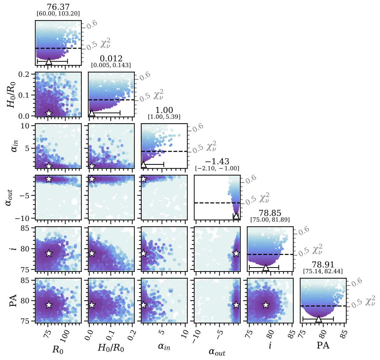
The key results of the four modeling procedures (two for RDI-KLIP, one for ADI-KLIP, and one combined) are provided in Table 2. A corner plot for the combined procedure is provided in Figure 5. For analysis hereafter (e.g. for attenuation correction in Section IV), we adopt the best-fitting model resulting for the combined procedure, having parameters: au, , , , and (visualized in Figures 6, 7). The results of the other modeling procedures are visualized and compared in Appendix A.
| (au) | (deg) | PA (deg) | |||||
|---|---|---|---|---|---|---|---|
| RDI-KLIP (1) | 75.4 | 0.007 | 1.0 | -1.4 | 78.9 | 79.0 | 0.45 |
| N=1980 | [60.0, 103.2] | [0.005, 0.143] | [1.0, 5.0] | [75.0, 81.4] | [75.1, 82.4] | <0.50 | |
| RDI-KLIP (2) | 76.4 | 0.012 | 1.0 | -1.4 | 78.9 | 78.9 | 0.45 |
| N=2340 | [60.0, 102.7] | [0.005, 0.138] | [1.0, 5.4] | [75.0, 81.9] | [75.5, 82.4] | <0.50 | |
| ADI-KLIP | 87.4 | 0.005 | 1.0 | -1.6 | 79.3 | 80.6 | 0.76 |
| N=1800 | [70.3, 114.6] | [0.005, 0.050] | [1.0, 1.9] | [76.9, 81.3] | [78.7, 82.6] | <0.81 | |
| ADI & RDI | 82.7 | 0.005 | 1.0 | -1.5 | 79.1 | 80.1 | 0.61 |
| N=2160 | [64.1, 109.0] | [0.005, 0.052] | [1.0, 1.9] | [77.3, 80.7] | [78.6, 82.0] | <0.65 | |
| Currie et al. (2017) a | 75.6 | 0.118 | 3 | -3 | 75 | 75 | 1.03 |
| [66.7, 84.5] | [0.070, 0.160] | [3, 10] | [70, 75] | <1.07 | |||
| Bounds | – |
Note. — Results for each of the four distinct DE optimization runs outlined in Section III.1, as well as the forward modeling of HD 36546 in Currie et al. 2017. Each parameter column provides the value for the best model for the run indicated in the leftmost column (with indicating the total number of models evaluated for each procedure), with the following line providing the range of values resulting in an acceptably fitting model. The final column gives the corresponding run’s minimum and the threshold for acceptable models. The permitted boundary for each parameter in modeling for CHARIS data (the modeling procedure of Currie et al. 2017 used different bounds) is given on the final line. We adopt the best model for the combined run (“ADI & RDI”) for analysis hereafter. In Currie et al. 2017, models are discussed in terms of ( or in the text) rather than ; for simplicity we present these results in terms of instead. Additionally, we have updated relevant values for the difference in the assumed distance to the system — 114 pc in Currie et al. 2017, versus 101.35 pc here.


III.3 Modeling Discussion
The results of our forward-modeling procedure echo many of the themes of the results in Currie et al. 2017: favoring a highly inclined disk model with shallow radial density profiles (small , ), suggestive of an extended disk as opposed to the ring-like geometry often found for debris disks.
We emphasize here that, while the nominal parameter values are expected to very closely correspond to the global minimum of the parameter space, the acceptable parameter ranges from DE provide only a rough approximation of parameter uncertainties. Unlike ensemble samplers (e.g. Markov chain Monte Carlo), which draw samples from a parameter space in proportion to the statistical likelihood of those samples, DE is designed to rapidly approach the global minimum with little regard for sub-optimal combinations of parameters; in cases where the algorithm identifies a strong value for a particular parameter early in the run, the values of that parameter which yield “acceptable” results may be poorly explored. If a stronger approximation of parameter uncertainties is desired, repeated DE runs (or follow-up runs near the best DE solution with “local” optimization algorithms, such as damped least-squares) can provide thorough exploration of acceptable values while still requiring orders of magnitude fewer samples than would be required by an ensemble sampler.
While highly inclined disks are expected to be relatively insensitive to changes in the parameters (see, e.g., Lawson et al. 2020), these parameters are perhaps the best constrained of any in our modeling (see Figure 5). This might be explained by the particularly small scale height favored by our modeling: , an order of magnitude smaller than the median value of 0.06 provided by Hughes et al. 2018 and the lower boundary for values permitted by our procedure. However, we note that scale heights up to are also acceptable solutions. In fact, the diagonal subplot for in Figure 5 shows that the minimum changes very little as a function of for . Given that the corner plot shows no obvious strong correlations between and other parameters, this appears to suggest that our data simply cannot discriminate between values in this range. This is not particularly surprising, given that for a fiducial radius of au corresponds to au, which projects to or pixels, compared to our resolution of pixels. Considering this apparent degeneracy for , our results for this parameter should be interpreted as . Additionally, we note that the value of converges to the lower bound for permitted values (). This result, indicating an exceptionally slow decline in density interior to , could suggest that the disk is better described by a geometry with a nearly flat density slope over some intermediate region, followed by typical power-law slopes interior and exterior to that region. An alternative explanation for the strong constraint that manifests here is addressed briefly in Section IV.1.
The best-fit parameter values and acceptable ranges resulting from forward modeling in Currie et al. 2017 are included for comparison in Table 2. Notably, this modeling was conducted on a coarse grid; the acceptable ranges provided are much less likely to correspond to complete ranges of acceptably-fitting parameters. Additionally, we note that, while the value for PA identified in Currie et al. 2017 is at the lower bound of allowed values for our presented DE runs, in earlier modeling runs not presented here the range of allowed PA values extended as low as 60 but showed very poor fits for PA . As such, the final procedure restricted PA to the provided range to speed convergence. As stated previously, our results are thematically consistent with the picture of the disk suggested by the analysis in Currie et al. 2017. Many of the specific parameter values identified, however, appear inconsistent; e.g., despite evaluating models with , the best-fit in Currie et al. 2017 is achieved for . Forward modeling the best fit solution from Currie et al. 2017 for our reductions results in a combined value of (well beyond the limit for acceptable models of ). This apparent difference in identified optimal parameters might be explained by some combination of a few key differences in the modeling procedures:
- 1.
the data itself, e.g. with the CHARIS reduction making a partial detection of the fainter side of the disk where HiCIAO data did not,
- 2.
the scattering phase functions, with our choice to adopt the Hong phase function, as opposed to fitting an asymmetry parameter as in Currie et al. 2017; in prior work modeling the disk of HD 15115 (Lawson et al. 2020), this was found to have a significant impact on the optimal parameters,
- 3.
the choice in Currie et al. 2017 to not vary PA, instead adopting the PA resulting from spine tracing,
- 4.
the parameter bounds, e.g. with values of in Currie et al. 2017 not including the best-fit value that we identify,
- 5.
the parameter optimization, with Currie et al. 2017 identifying best-fit parameters through a much less thorough grid search.
The best-fit model for the combined (“ADI & RDI”) DE run results in a reduced score for each reduction that is very similar to the best scores achieved in the DE runs for individual reductions. The DE run for only the ADI-KLIP reduction results in a best-fit model having (with “acceptable” models having ), while the best-fit model of the combined run results in when considering only the ADI-KLIP data — well within the limit to be considered an acceptable solution. Similarly, the DE runs for only the RDI-KLIP reduction result in a best-fit model having (with being acceptable) while the best-fit model of the combined run results in for the RDI-KLIP reduction. In other words, the adopted disk model from our combined modeling run is also a reasonable explanation when considering the imagery of each data reduction individually.
IV Disk Spine Trace and Surface Brightness
To measure the disk’s spine and surface brightness (SB), we proceed largely as detailed in Lawson et al. 2020 and summarized hereafter. In place of the RDI-KLIP reduction utilized for modeling, we perform spine fitting and surface brightness measurements on an RDI-KLIP reduction in which radial profile subtraction is utilized (with all other parameters remaining unchanged). This results in a generally weaker detection of the disk at very small separations and in wavelength collapsed imagery, but provides a more consistent detection across the field of view and in individual wavelength channels. For the sake of attenuation correction, we forward-model the adopted best-fitting model of Section III.1 for this additional reduction. The wavelength-collapsed image for this reduction and the corresponding forward modeling results are provided in Appendix B.
IV.1 Disk Spine
The positions of peak radial brightness along the disk are referred to as the disk’s spine, and are typically used as locations for surface brightness measurements and to approximate the geometric paramaters of the disk (e.g., fiducial radius, inclination, and position angle). We fit the spine position using wavelength-collapsed products and applying an initial image rotation of to approximately horizontally align the disk’s major-axis. We then measure the spine at each pixel column position by fitting Lorentzian profiles to the image values weighted by the inverse of the radial noise profile. The fit Lorentzian peak and associated fit uncertainty are taken as the spine position and uncertainty. As a departure from the method of Lawson et al. 2020, the fitting is carried out on both the ADI-KLIP and RDI-KLIP images simultaneously to identify the spine position most consistent with both images (rather than taking the weighted average of the results).
Notably, the fit spine (Figure 8) appears to grow further from the major axis at larger separations, suggesting a possible “swept-back wing” geometry (see e.g. Hughes et al. 2018), in which a disk’s outer dust ring appears to bend (rather than remaining planar) at increasing separations. As a result of this, the measured spine is extremely poorly described by an ellipse and thus cannot easily provide a meaningful assessment of the disk’s inclination or radius. While it may be possible to estimate the position angle of the disk’s major axis from this spine profile, it is unclear how the value would be affected by the noted phenomenon. As such, we provide no estimate of the disk geometry based on spine fitting. For the locations of surface brightness measurements, we use the fit spine profile in place of the best-fit ellipse profile used for our analysis in Lawson et al. 2020 — correcting the initial rotation of using a rotational transformation of the spine positions.
Interestingly, applying this spine fitting procedure to our best-fitting models also results in a divergent spine trace (both before and after attenuation is induced by forward modeling). After comparison to the complete sample of models, this behavior manifests only if . This could suggest that the observed spine shape is simply the result of a disk with a dust distribution meeting this criteria and viewed nearly edge-on. Alternatively, models having such values of may have been the only accessible means by which to reproduce this feature of the observations – with the true cause being more similar to the explanations summarized by Hughes et al. 2018 (e.g. ISM interaction).

IV.2 Disk Surface Brightness
Peak surface brightness is measured for both the RDI-KLIP and ADI-KLIP reductions at the aforementioned spine locations using an aperture of diameter 012 (7.4 pixels). As in Lawson et al. 2020, a) we apply wavelength-dependent attenuation corrections based the adopted disk model (determined by comparison of the PSF-convolved input model cube and the attenuated model cube after forward modeling), and b) we approximate the uncertainty for each SB measurement as the standard deviation of an array of like-measurements taken at the same stellocentric radius but with azimuthal angles placed every 10°. These measurements are made on the “broadband” wavelength-collapsed images, as well as images corresponding to , , and bands. The final surface brightness profile for a given filter is taken to be the weighted average of the results for the two individual reductions. The results of this procedure are visualized in Figure 10.
Disk surface contrast (the surface brightness of the disk relative to the stellar flux) is then computed by combining disk SB with measurements of the stellar flux for each filter (Figure 11).
Any east-west asymmetry is measured by comparing the surface brightness of opposing sides in a given filter (Figure 12).
Finally, the disk color in isolation from the stellar color is measured by converting surface contrasts to magnitudes and taking the difference of measurements between filters (see Figure 13), e.g. , where is the color of the disk without contribution from the star.
IV.3 Surface Brightness Power-Law
For the broadband (wavelength-collapsed) images, we make an additional set of measurements to facilitate fitting a power-law to the disk’s radial surface brightness profile. For this purpose, we follow the SB measurement procedure of Section IV.2, except:
- 1.
measurements are made at positions with an array of radial separations but corresponding to a single scattering angle (25°1010 10 The particular scattering angle is chosen arbitrarily in an attempt to probe a scattering angle providing radial coverage with both generally high disk signal and well defined attenuation estimates in the east and west. Values within provide comparable results., assuming and based on the results of Section III.2),
- 2.
images are binned to resolution ( pixels ),
- 3.
the aperture diameter is set to one resolution element
The first change enables characterization of the radial dependence of the disk’s SB for comparison with results in the literature, while the latter two changes result in approximately statistically independent SB measurements for fitting. The locations of these measurements are overlaid on the binned ADI-KLIP image in the top panel of Figure 14. We then fit power-laws to these SB measurements as a function of deprojected stellocentric separation1111 11 Derived deprojected stellocentric separations consider only the determined PA and inclination of the system, and assume that our line of sight probes light scattered from the disk midplane. A more detailed assessment would take scale height, flaring, and similar effects into account, but is beyond the scope of this work. for the eastern and western extents of the disk separately (Figure 14). We find best fitting power law slopes of and for the west and east respectively.

IV.4 Surface Brightness Discussion
Disk Color – Our individual measurements of disk color along the apparent spine of the disk (Figure 13) appear generally consistent with a disk scattering profile that is grey in NIR. However, taking the inverse-variance weighted average of the individual measurements for each color suggests a slightly blue color for the disk in both cases: and . 1212 12 This general result appears to be robust to the specific disk model adopted for the sake of attenuation correction. Calculating the average disk colors using each of the 691 acceptable disk models for attenuation correction instead resulted in color ranges of and with uncertainties comparable to the values found using the best-fit disk for attenuation correction. Notably, the locations of the apparent disk spine at which this blue color was measured fall beyond the projected location of peak density for the disk. To assess the properties of the bulk population of dust in the disk, rather than just those of the dust pushed to larger separations by pressure from the parent star, we make additional measurements of the disk’s color in the vicinity of the disk’s peak radial density. For this purpose, we measure surface brightness in apertures of the same size (006) along the brighter side of the disk at the projected location of the adopted disk model’s density peak (i.e., along the southern edge of the ellipse overlaid in Figure 8 – corresponding to a single deprojected stellocentric separation). From these measurements, we proceed to average color measurements as before, finding: , , and . These results again suggest a slightly blue NIR color for the disk.
Comparison with the numerical simulations in Boccaletti et al. 2003, which model NIR disk colors as a function of the dust size distribution’s minimum grain size () and porosity (P), can enable some constraints regarding the size distribution of the dust in HD 36546’s disk. With , for 1.1 versus 2.2 (), a blue disk color is achieved only for . Similarly, for 1.6 versus 2.2 () a blue color is achieved for µm. Finally, for 1.1 versus 1.6 (), a blue color is achieved for µm1313 13 The models of Boccaletti et al. 2003 are presented in terms of and . For our purposes, we combine the provided measurements to present these results in terms of as well. Based on these simulations, we can estimate a minimum grain size (assuming P=0) of to produce the blue color that we observe. The minimum grain size producing a blue color tends to increase for higher porosity, e.g. with producing a blue JK color for P=0.95.
Disk Asymmetry – Both individual measurements and the overall averages for east-west flux asymmetry show no statistically significant evidence for a disk that is asymmetric in brightness in any of the four filters analyzed (Figure 12). While the processed imagery of the disk may initially suggest some asymmetry is present – with the western extent of the disk appearing brighter in all three presented reductions in Figure 2 – no asymmetry is evident in SB measurements once attenuation corrections are applied. Thus, we conclude that the apparent asymmetry in CHARIS imagery is an artifact of PSF-subtraction and is not truly astrophysical in nature.
Disk Power-Law – The results of power-law fitting (Figure 14) are in good agreement with the results of our asymmetry measurements (Figure 12) — again suggesting that the disk’s flux is largely symmetrical at NIR wavelengths in the region of CHARIS’s detection.
Comparing our best-fitting power law slope of for HD 36546 ( au) to values in the literature for other debris disks provides further evidence that HD 36546 has a particularly shallow density slope. For the debris disk of HD 32297 ( au), Currie et al. 2012b find and for the debris disk of HR 4796 A ( au), Thalmann et al. 2011 report .
V Limits on Planets
For the planet detection reduction outlined in Section II.2, we computed contrast limits in CHARIS broadband, following the procedure of Currie et al. 2018 for computing planet throughput corrections.
Contrasts are about a factor of 2–3 worse at 075 than good performance for bright diskless stars (Currie et al. 2020a) and slightly poorer than our previous limits for the debris disk-bearing HD 15115 (Lawson et al. 2020). However, despite a loss of wavefront sensing sensitivity (see Section II), we reach contrasts at mid spatial frequencies slightly better than those achieved in Currie et al. 2017 with SCExAO/HiCIAO (e.g. at 045 with CHARIS, versus with HiCIAO). This gain is likely due to the use of SDI for additional speckle suppression.
To convert from contrast to planet mass limits, we integrated the hot-start, solar metallicity, hybrid cloud, synthetic planet spectra provided by Spiegel & Burrows 2012 over the CHARIS bandpass and divided by the integrated stellar spectrum. We consider two mappings between contrast and mass, corresponding to the lower and upper age limits estimated for the system (3 Myr and 10 Myr).
The right axis of Figure 15 denotes these mass limits. For au ( ), our reduction is sensitive to planets at Myr, and planets at Myr. Despite achieving generally inferior contrasts compared to the best reduction of CHARIS data for the debris disk-bearing star HD 15115 (Lawson et al. 2020), we are able to probe slightly less massive planets at a given projected separation due to HD 36546’s relative youth.
While our data do not result in the detection of any candidate planets, HD 36546 may show tentative, indirect evidence for a massive and (in-principle) imageable companion. The Hipparcos-Gaia Catalog of Accelerations (HGCA; Brandt 2018) provides calibrated proper motion data for nearby stars spanning the year baseline between Hipparcos and Gaia astrometry. Accelerations based on this data have been used to measure dynamical masses of directly imaged exoplanets (Brandt et al. 2019, e.g.), as well as to provide evidence of gravitational interaction with yet-unseen companions for targeted direct imaging searches (Currie et al. 2020b; Steiger et al. 2021). Brandt et al. (2021, submitted) updates HGCA, replacing Gaia DR2 measurements with those from Gaia eDR3, which yield a factor of 3 improvement in astrometric precision. Using these updated Gaia measurements, HGCA for HD 36546 (Table 3) indicates a marginally significant acceleration relative to a model of constant proper motion — , or 2.3 for two degrees of freedom — that could be indicative of a companion.
| Source | Corr | ||||||
|---|---|---|---|---|---|---|---|
| Hip | 8.513 | 0.974 | -41.876 | 0.472 | 0.257 | 1991.15 | 1990.76 |
| HG | 7.368 | 0.028 | -41.226 | 0.014 | 0.087 | ||
| Gaia | 7.508 | 0.056 | -41.305 | 0.040 | -0.137 | 2016.00 | 2016.50 |
Note. — HGCA calibrated proper motion measurements for HD 36546 (Brandt 2018) as updated with Gaia eDR3 measurements in Brandt et al. (2021, submitted).
Following equations in Brandt et al. 2019 to estimate companion mass as a function of projected separation using HGCA accelerations, we can assess the completeness of our search for the HD 36546 companion that would induce this acceleration. Since radial velocity (RV) measurements are not available for HD 36546, we adopt an RV acceleration of zero to compute a minimum mass instead. Mapping of the resulting minimum masses to contrasts for 3 Myr and 10 Myr are overlaid on Figure 15. These results suggest that we would likely recover the HGCA companion for a projected separation beyond assuming an age of 3 Myr, or for an age of 10 Myr.
VI Conclusions and Future Work
Our study provides the first multi-wavelength imaging of the HD 36546 disk and recovers disk signal to separations as small as . Through detailed modeling implementing a Hong 1985 scattering phase function and using the differential evolution optimization algorithm, we provide an updated schematic of HD 36546’s disk. This schematic suggests a disk with a particularly shallow radial dust density profile, a fiducial radius of au, an inclination of , and a position angle of . Through spine tracing, we find a disk spine that is consistent with our modeling results, but also consistent with a “swept-back wing” geometry. Surface brightness measurements show no significant flux asymmetry between the eastern and western extents of the disk, and slightly blue NIR colors on average. While we report no evidence of directly imaged companions, we provide contrast limits to constrain the most plausible remaining companions.
Notably, prior work modeling the debris disks of HD 36546 and HD 15115 in NIR total intensity data identified very distinct optimal HG SPF asymmetry parameters of (Currie et al. 2017) and (Engler et al. 2019) respectively. Alongside the results of Lawson et al. 2020, we have shown that imagery of both disks can be reasonably reproduced by models using the same Hong 1985 SPF instead. As is suggested in Hughes et al. 2018, this may support the existence of a nearly universal SPF for circumstellar dust. Additional data to study smaller scattering angles and additional disk systems is necessary to clarify this possibility. If such an SPF is verified, it will enable both better exploration of model parameters (by reducing the number of varying parameters) and tighter constraints on parameter values (by mitigating parameter degeneracies).
Deeper follow-up observations with SCExAO/CHARIS would provide a) further constraints on companions within the disk and b) higher SNR measurements of the disk color, enabling a more detailed assessment of the dust properties of the disk. The upcoming replacement of Subaru’s AO188 system and additional commissioned improvements to wavefront sensing are expected to improve SCExAO/CHARIS contrasts at small separations by roughly a factor of 10 by late 2021 (Currie et al. 2020a). Assuming a system age of 3 Myr, these contrasts would enable detection of 1 -mass planets at au. A future non-detection would likely restrict the location of any super-Jovian mass planet to .
Observations measuring the polarized intensity of the disk at comparable scales – or the total intensity of the disk in a wider field of view – could clarify the underlying cause of the noted diverging spine trace. CHARIS’s integral field spectropolarimetry mode or space-based imaging of the system could provide these data. Further, polarized intensity imaging would enable even tighter constraints on disk model parameters by better probing regions of the disk where the polarized intensity phase function results in more favorable sensitivity.
Appendix A Additional Model Results
The results of our additional differential evolution disk model optimization procedures are included here, with the information of Table 2 graphically summarized in Figure 16. Individual reductions are in close agreement with one another; while the optimal values for some parameters (e.g. ) differ noticeably compared to the permitted parameter bounds, each reduction’s best fit values fall within the acceptable ranges for the other reductions.
Comparison of the samples for between the two RDI-KLIP DE runs (the first two rows of Figure 16) illustrates our prior warning regarding approximation of parameter uncertainties from DE (see Section III.3). While the runs ultimately yield very similar acceptable ranges, the comparable upper limit achieved for “RDI-KLIP (2)” is the result of a single sample; except for the lone acceptable model with , the acceptable range of values for this run would manifest much more comparably to that of the ADI-KLIP run.
As a result of the larger noise levels in the RDI-KLIP reduction, the RDI-KLIP modeling procedure (Fig. 17) shows much weaker constraints than the ADI-KLIP (Fig. 18) modeling procedure. Despite some differences in the resulting parameter values, the best-fit solutions for these procedures manifest very similarly to those of the combined run (e.g. Figures 6, 7).


Appendix B RDI-KLIP Reduction using Radial Profile Subtraction
The results of forward modeling the adopted best-fitting model for the radial profile subtracted RDI-KLIP reduction (see Section IV) are provided in Figure 19.

References
- Augereau et al. (1999) Augereau, J. C., Lagrange, A. M., Mouillet, D., Papaloizou, J. C. B., & Grorod, P. A. 1999, A&A, 348, 557. https://arxiv.org/abs/astro-ph/9906429
- Beuzit et al. (2019) Beuzit, J. L., Vigan, A., Mouillet, D., et al. 2019, A&A, 631, A155, doi: 10.1051/0004-6361/201935251
- Boccaletti et al. (2003) Boccaletti, A., Augereau, J. C., Marchis, F., & Hahn, J. 2003, ApJ, 585, 494, doi: 10.1086/346019
- Brandt (2018) Brandt, T. D. 2018, ApJS, 239, 31, doi: 10.3847/1538-4365/aaec06
- Brandt et al. (2019) Brandt, T. D., Dupuy, T. J., & Bowler, B. P. 2019, AJ, 158, 140, doi: 10.3847/1538-3881/ab04a8
- Brandt et al. (2017) Brandt, T. D., Rizzo, M., Groff, T., et al. 2017, Journal of Astronomical Telescopes, Instruments, and Systems, 3, 048002, doi: 10.1117/1.JATIS.3.4.048002
- Chen et al. (2020) Chen, C., Mazoyer, J., Poteet, C. A., et al. 2020, ApJ, 898, 55, doi: 10.3847/1538-4357/ab9aba
- Cloutier et al. (2014) Cloutier, R., Currie, T., Rieke, G. H., et al. 2014, ApJ, 796, 127, doi: 10.1088/0004-637X/796/2/127
- Currie et al. (2015a) Currie, T., Cloutier, R., Brittain, S., et al. 2015a, ApJ, 814, L27, doi: 10.1088/2041-8205/814/2/L27
- Currie et al. (2008) Currie, T., Kenyon, S. J., Balog, Z., et al. 2008, ApJ, 672, 558, doi: 10.1086/523698
- Currie et al. (2009) Currie, T., Lada, C. J., Plavchan, P., et al. 2009, ApJ, 698, 1, doi: 10.1088/0004-637X/698/1/1
- Currie et al. (2015b) Currie, T., Lisse, C. M., Kuchner, M., et al. 2015b, ApJ, 807, L7, doi: 10.1088/2041-8205/807/1/L7
- Currie et al. (2011) Currie, T., Burrows, A., Itoh, Y., et al. 2011, ApJ, 729, 128, doi: 10.1088/0004-637X/729/2/128
- Currie et al. (2012a) Currie, T., Debes, J., Rodigas, T. J., et al. 2012a, ApJ, 760, L32, doi: 10.1088/2041-8205/760/2/L32
- Currie et al. (2012b) Currie, T., Rodigas, T. J., Debes, J., et al. 2012b, ApJ, 757, 28, doi: 10.1088/0004-637X/757/1/28
- Currie et al. (2017) Currie, T., Guyon, O., Tamura, M., et al. 2017, ApJ, 836, L15, doi: 10.3847/2041-8213/836/1/L15
- Currie et al. (2018) Currie, T., Brandt, T. D., Uyama, T., et al. 2018, AJ, 156, 291, doi: 10.3847/1538-3881/aae9ea
- Currie et al. (2019) Currie, T., Marois, C., Cieza, L., et al. 2019, ApJ, 877, L3, doi: 10.3847/2041-8213/ab1b42
- Currie et al. (2020a) Currie, T., Guyon, O., Lozi, J., et al. 2020a, in Society of Photo-Optical Instrumentation Engineers (SPIE) Conference Series, Vol. 11448, Society of Photo-Optical Instrumentation Engineers (SPIE) Conference Series, 114487H, doi: 10.1117/12.2576349
- Currie et al. (2020b) Currie, T., Brandt, T. D., Kuzuhara, M., et al. 2020b, ApJ, 904, L25, doi: 10.3847/2041-8213/abc631
- Duchêne et al. (2020) Duchêne, G., Rice, M., Hom, J., et al. 2020, AJ, 159, 251, doi: 10.3847/1538-3881/ab8881
- Engler et al. (2019) Engler, N., Boccaletti, A., Schmid, H. M., et al. 2019, A&A, 622, A192, doi: 10.1051/0004-6361/201833542
- Esposito et al. (2020) Esposito, T. M., Kalas, P., Fitzgerald, M. P., et al. 2020, AJ, 160, 24, doi: 10.3847/1538-3881/ab9199
- Fitzgerald et al. (2007) Fitzgerald, M. P., Kalas, P. G., Duchêne, G., Pinte, C., & Graham, J. R. 2007, ApJ, 670, 536, doi: 10.1086/521344
- Gagné et al. (2018) Gagné, J., Mamajek, E. E., Malo, L., et al. 2018, ApJ, 856, 23, doi: 10.3847/1538-4357/aaae09
- Gaia Collaboration et al. (2018) Gaia Collaboration, Brown, A. G. A., Vallenari, A., et al. 2018, A&A, 616, A1, doi: 10.1051/0004-6361/201833051
- Gibbs et al. (2019) Gibbs, A., Wagner, K., Apai, D., et al. 2019, AJ, 157, 39, doi: 10.3847/1538-3881/aaf1bd
- Goebel et al. (2018) Goebel, S., Currie, T., Guyon, O., et al. 2018, AJ, 156, 279, doi: 10.3847/1538-3881/aaeb24
- Groff et al. (2016) Groff, T. D., Chilcote, J., Kasdin, N. J., et al. 2016, in Society of Photo-Optical Instrumentation Engineers (SPIE) Conference Series, Vol. 9908, Ground-based and Airborne Instrumentation for Astronomy VI, 99080O, doi: 10.1117/12.2233447
- Henyey & Greenstein (1941) Henyey, L. G., & Greenstein, J. L. 1941, ApJ, 93, 70, doi: 10.1086/144246
- Hong (1985) Hong, S. S. 1985, A&A, 146, 67
- Hughes et al. (2018) Hughes, A. M., Duchêne, G., & Matthews, B. C. 2018, ARA&A, 56, 541, doi: 10.1146/annurev-astro-081817-052035
- Jovanovic et al. (2015) Jovanovic, N., Martinache, F., Guyon, O., et al. 2015, PASP, 127, 890, doi: 10.1086/682989
- Kalas et al. (2005) Kalas, P., Graham, J. R., & Clampin, M. 2005, Nature, 435, 1067, doi: 10.1038/nature03601
- Kenyon & Bromley (2008) Kenyon, S. J., & Bromley, B. C. 2008, ApJS, 179, 451, doi: 10.1086/591794
- Lafrenière et al. (2007) Lafrenière, D., Marois, C., Doyon, R., Nadeau, D., & Artigau, É. 2007, ApJ, 660, 770, doi: 10.1086/513180
- Lagrange et al. (2010) Lagrange, A.-M., Bonnefoy, M., Chauvin, G., et al. 2010, Science, 329, 57, doi: 10.1126/science.1187187
- Lawson et al. (2020) Lawson, K., Currie, T., Wisniewski, J. P., et al. 2020, AJ, 160, 163, doi: 10.3847/1538-3881/ababa6
- Lisse et al. (2017) Lisse, C. M., Sitko, M. L., Russell, R. W., et al. 2017, ApJ, 840, L20, doi: 10.3847/2041-8213/aa6ea3
- Lozi et al. (2018) Lozi, J., Guyon, O., Jovanovic, N., et al. 2018, in Society of Photo-Optical Instrumentation Engineers (SPIE) Conference Series, Vol. 10703, Proc. SPIE, 1070359, doi: 10.1117/12.2314282
- Macintosh et al. (2015) Macintosh, B., Graham, J. R., Barman, T., et al. 2015, Science, 350, 64, doi: 10.1126/science.aac5891
- Marois et al. (2006) Marois, C., Lafrenière, D., Doyon, R., Macintosh, B., & Nadeau, D. 2006, ApJ, 641, 556, doi: 10.1086/500401
- Marois et al. (2010) Marois, C., Macintosh, B., & Véran, J.-P. 2010, in Society of Photo-Optical Instrumentation Engineers (SPIE) Conference Series, Vol. 7736, Proc. SPIE, 77361J, doi: 10.1117/12.857225
- Mawet et al. (2014) Mawet, D., Milli, J., Wahhaj, Z., et al. 2014, ApJ, 792, 97, doi: 10.1088/0004-637X/792/2/97
- Millar-Blanchaer et al. (2015) Millar-Blanchaer, M. A., Graham, J. R., Pueyo, L., et al. 2015, ApJ, 811, 18, doi: 10.1088/0004-637X/811/1/18
- Milli et al. (2017) Milli, J., Vigan, A., Mouillet, D., et al. 2017, A&A, 599, A108, doi: 10.1051/0004-6361/201527838
- Pueyo (2016) Pueyo, L. 2016, ApJ, 824, 117, doi: 10.3847/0004-637X/824/2/117
- Ribas et al. (2015) Ribas, Á., Bouy, H., & Merín, B. 2015, A&A, 576, A52, doi: 10.1051/0004-6361/201424846
- Schneider et al. (2014) Schneider, G., Grady, C. A., Hines, D. C., et al. 2014, AJ, 148, 59, doi: 10.1088/0004-6256/148/4/59
- Smith & Terrile (1984) Smith, B. A., & Terrile, R. J. 1984, Science, 226, 1421, doi: 10.1126/science.226.4681.1421
- Soummer et al. (2012) Soummer, R., Pueyo, L., & Larkin, J. 2012, ApJ, 755, L28, doi: 10.1088/2041-8205/755/2/L28
- Sparks & Ford (2002) Sparks, W. B., & Ford, H. C. 2002, ApJ, 578, 543, doi: 10.1086/342401
- Spiegel & Burrows (2012) Spiegel, D. S., & Burrows, A. 2012, ApJ, 745, 174, doi: 10.1088/0004-637X/745/2/174
- Steiger et al. (2021) Steiger, S., Currie, T., Brandt, T. D., et al. 2021, AJ, 162, 44, doi: 10.3847/1538-3881/ac02cc
- Thalmann et al. (2011) Thalmann, C., Janson, M., Buenzli, E., et al. 2011, ApJ, 743, L6, doi: 10.1088/2041-8205/743/1/L6
- Thalmann et al. (2013) —. 2013, ApJ, 763, L29, doi: 10.1088/2041-8205/763/2/L29
- Wyatt (2008) Wyatt, M. C. 2008, ARA&A, 46, 339, doi: 10.1146/annurev.astro.45.051806.110525