∎
Convex Formulation for Planted Quasi-Clique Recovery
Abstract
In this paper, we consider the planted quasi-clique or -clique problem. This problem is an extension of the well known planted clique problem which is NP-hard. The maximum quasi-clique problem is applicable in community detection, information retrieval and biology. We propose a convex formulation using nuclear norm minimization for planted quasi-clique recovery. We carry out numerical experiments using our convex formulation and the existing mixed integer programming formulations. Results show that the convex formulation performs better than the mixed integer formulations when is greater than a particular threshold.
Keywords:
Quasi-clique Relaxations Nuclear norm Edge density1 Introduction
A clique is the densest subgraph of any undirected graph, . A subgraph, induced by , forms a clique if every pair of nodes are adjacent Luce and Perry 1949. The problem of finding the largest clique in a graph is known as the Maximum Clique Problem (MCP) Bomze et al. 1999; Pardalos and Rodgers 1992; Pardalos and Xue 1994. The size of the largest clique in is known as the clique number and it is denoted by . Although this problem is NP-hard Garey and Johnson 2002, it has been well studied due to its wide applications. Verily, cliques possess the ideal properties for cohesiveness Pattillo et al. 2012. However, the requirement that every pair of nodes are adjacent is too confining for some applications Pattillo et al. 2013. This motivates the emergence of different clique relaxations. Some of the clique relaxation models emanating from soical network analysis include the -clique, -club, and -plex, see for example, Balasundaram et al. 2005; Balasundaram et al. 2011. A density based relaxation known as quasi-clique or -clique was introduced in Abello et al. 1999. Although -clique is the most recent of clique relaxations, it is one of the most popular due to its suitability for a range of applications Veremyev et al. 2016. The quasi-clique model is applicable in community detection Hajek et al. 2015; Pattillo et al. 2012, data clustering and data mining Balasundaram et al. 2005; Verma and Butenko 2013, information retrieval Terveen et al. 1999, protein-protein network Junker and Schreiber 2011, and criminal network analysis Balabhaskar 2007; Kiani et al. 2015.
A subgraph, , is a -clique if , where . The problem of finding a -clique with maximum cardinality in is known as the maximum quasi-clique problem (MQCP). Obviously, the case is equivalent to the maximum clique problem. This problem has been shown to be NP-hard Pattillo et al. 2013. The size of the maximum quasi-clique in is known as -clique number and we denote it by . A number of existing works on finding the maximum -clique focused on developing heuristic methods for finding large quasi-cliques for different instances Abello et al. 2002; Bhattacharyya and Bandyopadhyay 2009; Liu and Wong 2008; Pei et al. 2005. Other various heuristic and enumerative algorithms have recently been developed (see e.g, Marinelli et al. 2020; Miao and Balasundaram 2020; Pastukhov et al. 2018; Ribeiro and Riveaux 2019; Zhou et al. 2020)
The first mathematical model for maximum quasi-clique recovery is the mixed integer programming (MIP) of Pattillo et al. 2013. This model has been reformulated in Veremyev et al. 2016 to handle larger problems. These are the only known existing maximum quasi-clique recovery models. In this paper, we focus on a special case of this problem, namely, the planted quasi-clique. We propose a novel convex formulation for the planted quasi-clique recovery. We adopt techniques from the matrix decomposition to split the adjacency matrix of the given graph into its low rank and sparse component. We were inspired by the work in Ames and Vavasis 2011 where a matrix completion strategy was used for planted maximum clique recovery. Planted clique is a well known problem that has been studied in Alon et al. 1998; Ames and Vavasis 2011; Frieze and Kannan 2008; Kučera 1995. To the best of our knowledge, this paper presents the first attempt to solve the planted maximum -clique problem. Our numerical experiments show that this approach is more robust than the nuclear norm formulation of Ames and Vavasis 2011 and more effective for planted quasi-clique recovery than the mixed integer programming models of Pattillo et al. 2013; Veremyev et al. 2016.
The rest of this paper is organised as follows. We present the nuclear norm formulation for the planted clique and planted quasi-clique problem in Section 2. We briefly present the mixed integer programming formulations for maximum quasi-clique problem in Section 4. The report of our numerical experiments is presented in Section 5 while the concluding remarks are made in Section 6.
2 The planted quasi-clique model
An instance of the MCP is the planted (hidden) clique problem. The problem can be formulated in two different ways namely: the randomized case and the adversarial case. For the randomized case, vertices are chosen at random from vertices () and a clique of size is constructed. The remaining pairs of nodes are then connected depending on a given probability. For the adversarial case, on the contrary, instead of joining the diversionary edges in a probabilistic manner, an adversary is allowed to join the edges. A restriction is placed on the maximum number of edges he can insert so that a clique bigger than the planted clique is not formed. For our planted quasi-clique problem, we have only considered the randomized case. We have formulated the problem using two probablities, namely: , is the probability of an edge existing between two nodes belonging to the planted quasi-clique while is the probability of an edge between the nodes not belonging to the planted quasi-clique. So, summarily, we generate a graph of size and select nodes randomly () and connect them with probability . The remaining nodes form the diversionary nodes are they are connected with probability . The smaller the value of the more difficulty it is to recover the planted quasi-clique. Conversely, as grows bigger, tending towards , the harder it is to recover the planted quasi-clique.
The planted clique problem has previously been studied in Alon et al. 1998; Feige and Krauthgamer 2000; Frieze and Kannan 2008; Kučera 1995. The following nuclear norm minimization formulation has been recently proposed for solving the planted clique problem Ames and Vavasis 2011:
| (1a) | ||||
| subject to | (1b) | |||
| (1c) | ||||
| (1d) | ||||
| (1e) | ||||
where and is the size of the planted clique. The nuclear norm is defined as , where , are the singlular values and is the rank of the matrix. We denote model (1) as NNM(1) (nuclear norm based model 1).
In our case, we adopt the technique from matrix decomposition Candès et al. 2011 to recover the planted quasi-clique in a graph. The planted quasi-clique problem is a more difficult problem than the planted clique problem, as the latter is a special case of the former. The matrix decomposition problem is described as follows. A matrix, , is formed by adding a low rank matrix, , to a sparse matrix, . The objective is to devise a mean to separate into its low rank and sparse component. Mathematically, we want to solve:
| (2a) | ||||
| (2b) | ||||
where is the number of non-zero entries of . Both the rank function and minimization are non-convex. However, nuclear norm minimization gives a good approximation of the rank minimization problem Recht et al. 2010. Furthermore, the matrix norm, defined as for , is a good replacement for the cardinality minimization problem Fornasier 2010. Hence, problem (2) can be written as
| (3a) | ||||
| (3b) | ||||
This problem has applications in facial recognition and image segmentation Candès et al. 2011. The problem has been studied in Candès et al. 2011; Chandrasekaran et al. 2011; Chen et al. 2013, with application to facial recognition in Candès et al. 2011. We apply this technique to planted quasi-clique recovery. Our proposed formulation is the following:
| (4a) | ||||
| subject to | (4b) | |||
| (4c) | ||||
| (4d) | ||||
where are matrix variables corresponding to the quasi-clique and the diversionary edges, is the adjacency matrix of the input graph while the parameter is the desired edge density of the quasi-clique to be recovered. The constraint (4b) enusures that the solution satisfies the edge density requirement, while (4c) makes sure that the decomposition agrees with the input matrix. is a positive integer value variable that determines the size of the recovered quasi-clique.
Since we are only interested in , we can eliminate constraint (4c) and write . Therefore, (4) can be reformulated as
| (5a) | ||||
| subject to | (5b) | |||
| (5c) | ||||
We denote model (5) as NNM(5). Following the approach in Appendix A of Chandrasekaran et al. 2011, the semidefinite (SDP) formulation for (5) is the following:
| (6) | ||||
where is an -dimensional vector of all entries equal to one and .
3 Illustrative Example
Suppose the input graph, , containing the planted quasi clique is the graph presented in Figure 1 and that we want to recover the planted -clique from it. is the adjacency matrix of . We add a loop to every node of to obtain as the adjacency matrix. This is necessary for the algorithm to be able to recover a low rank submatrix.
The matrix decomposition algorithm will perform two tasks, namely; completion of the low-rank matrix and separation of the low-rank matrix from the sparse matrix. However, since we are only interested in the low-rank submatrix, we have reformulated the model to suite this purpose. The reformulation has improved the performance of the algorithm in terms of speed. Therefore, for this particular example, we recover as the largest rank-one matrix and in this case. This corresponds to the adjacency matrix of the recovered maximum clique. The adjacency matrix of the planted maximum quasi-clique, , can then finally be obtained by setting if .

4 Existing Formulations for Maximum Quasi-Clique Problem
As stated earlier, majority of the existing works on -clique focused on developing heuristics for detection of large quasi-clique. The first deterministic solution for -clique recovery problem is based on the linear mixed integer programming model suggested in Pattillo et al. 2013, where an upper bound was derived. For , define such that if and only if and otherwise, where is the vertex set of the maximum quasi-clique. The following linearized MIP formulation was proposed:
| (7a) | ||||
| subject to: | ||||
| (7b) | ||||
| (7c) | ||||
| (7d) | ||||
| (7e) | ||||
| (7f) | ||||
where, are the entries of the adjacency matrix of the graph, is a constant that is large enough and is defined as
| (8) |
(7) can only handle problems with small graph size. Because of this drawback, Veremyev et al. 2016 Veremyev et al. 2016 reformulate this model by defining as a binary variable, such that if and only if . In addition, a binary variable , which determines the size of the quasi-clique is defined. This implies that if and only if . With these additional variables and notations, the improved MIP model presented in Veremyev et al. 2016 is:
| (9a) | ||||
| subject to | (9b) | |||
| (9c) | ||||
| (9d) | ||||
| (9e) | ||||
| (9f) | ||||
where and are the upper and lower bound on the size of quasi-clique that could be found in the input graph. These can be set to and respectively if no estimates are available. The constraint (9b) is the edge density requirement while (9c) ensures that if and only if and belong to the quasi-clique. Observe that the left hand side of (9b) can be written as
| (10) |
Setting to the quantity in the bracket in equation (10) above, (9) can be reformulated as Veremyev et al. 2016:
| (11a) | ||||
| subject to | (11b) | |||
| (11c) | ||||
| (11d) | ||||
| (11e) | ||||
| (11f) | ||||
where is a parameter that is sufficiently large. In particular, , where is the degree of a node in a given graph, .
5 Numerical Experiments
Recall that the planted quasi-clique problem becomes planted clique problem when is equal to one. We performed numerical experiments with our nuclear norm minimization (NNM) formulation (5) for planted maximum quasi-clique to compare its performance with the existing nuclear norm minimization formulation (1) for planted maximum clique recovery. Further, we compare the efficacy of our formulation with the mixed integer programming models (7), (9) and (11) for quasi cliques.
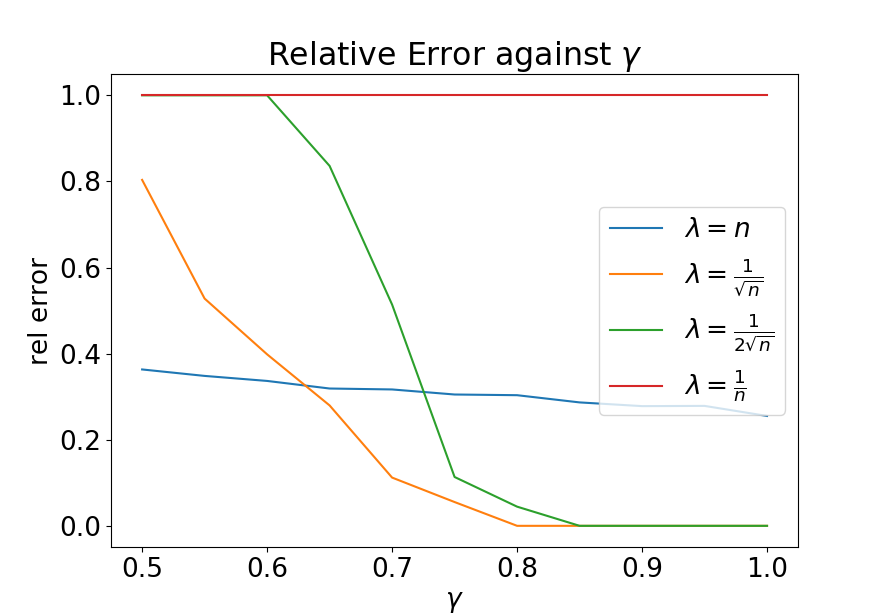
The experiments have been performed on a HP computer with 16GB Ram and Intel core i7 processor. The machine runs on Debian Linux. The simulations are performed using CVXPY Diamond and Boyd 2016 with NCVX Diamond et al. 2018. CVXPY is a python package used to solve convex optimization problems with different solvers, e.g SCS, CVXOPT, and XPRESS. Every instance of the experiment has been carried out ten times and the average result is taken. We have used different values of the regularization parameter, , to ascertain that our choice of works well for the problem. We have planted a quasi-clique with for various values of in a graph with nodes. We implement our algorithm for . The results is presented in Table 1 and Figure 2. From Table 1, we discover that when , the algorithm fails in all instances considered. This finding has been supported by the relative errors in Figure 2, where the relative errors have been calculated using (12).
| (12) |
where denotes the Frobenius norm. This is contrary to what can be observed when . For these values, the exact size of planted quasi-clique has been recovered with zero relative error when approaches (). From this results, we conclude that values of will work for our model. This is similar to the recommendation in Candès et al. 2011. This is not surprising since the entries of our matrix are also independent and identically distributed (iid) and hence satisfy the incoherence condition (see Candes and Plan 2010; Candés and Recht 2009; Candès et al. 2011). Chandrasekaran et al. 2011 Chandrasekaran et al. 2011 also contains a heuristic for choosing and our finding agrees with their result, although our approach is different. The detailed report of the experiments is as follows.
| Size of the planted quasi-clique | Size of recovered quasi-clique when | ||||
| 0.5 | 35 | 50 | 22.7 | 0 | 0 |
| 0.55 | 35 | 50 | 31 | 0 | 0 |
| 0.6 | 35 | 50 | 33.9 | 0 | 0 |
| 0.65 | 35 | 50 | 34.5 | 12.1 | 0 |
| 0.7 | 35 | 50 | 34.5 | 29.9 | 0 |
| 0.75 | 35 | 50 | 34.7 | 34.6 | 0 |
| 0.8 | 35 | 50 | 35 | 35 | 0 |
| 0.85 | 35 | 50 | 35 | 35 | 0 |
| 0.9 | 35 | 50 | 35 | 35 | 0 |
| 0.95 | 35 | 50 | 35 | 35 | 0 |
| 1 | 35 | 50 | 35 | 35 | 0 |
5.1 Comparison between NNM(1) and NNM(5)
Our model, NNM(5), represents the planted maximum clique model when . Hence, we compare its performance with NNM(1). We have considered a graph with 100 nodes in this experiment. We have planted clique of size and and then varied the probability, , of an edge existing between the remaining nodes. The results of this experiment is contained in Figure 3. In both cases considered, the results show that both (1) and (5) recover planted clique perfectly when the probability of adding a diversionary edge is below certain threshold (roughly ). However, (5) fails to perfectly recover the planted clique when this threshold is exceeded while (1) still solves the problem perfectly. We have observed that the presence of constraint (1c) enables finding the largest rank-one submatrix in the input matrix easier in the formulation (1). However, this constraint can not be imposed in the case of (5), otherwise, solving planted quasi-clique problem with the formulation will be impossible. Figure 4 represents the CPU times for NNM(1) and NNM(5) with planted clique of size and . It can be observed from the figures that NNM(1) is more efficient than NNM(5) in this case.
Figure 5 shows the performance of NNM(1) compared with NNM(5) in finding quasi-clique (with ). We have observed from Figure 5a that despite the fact that the planted quasi-clique that we have considered for this case has very few missing edges (), NNM(1) failed to recover the quasi-clique for every trial. However, NNM(5) produced similar result as the case (see Figure 3b and 5a). In addition, NNM(5) is, by far, more efficient than NNM(1) for the case (see Figure 5b).


5.2 Maximum Quasi-Clique Recovery
5.2.1 The planted case
Two types of experiment have been performed in this case. In the first case, we have checked whether the recovered quasi-clique satisfies the edge density requirement or not. The second experiment focuses on the size of the recovered quasi-clique, i.e, to examine whether the size of the planted quasi-clique () is the same as the size of the recovered quasi-clique (). The detailed report of both experiments is as follows.
The goal of the first experiment is to examine the error in the edge density of the recovered -clique with respect to the edge density of the planted maximum -clique. We have computed the relative error between the edge density of the recovered -clique and the edge density of the planted -clique (i.e, the expected edge density) for various . All the errors computed in this section are relative errors.
We have considered again graphs with and nodes for this case with planted -cliques of sizes and , respectively. The planted -clique corresponds to a dense submatrix of the (respectively, ) input matrix with (respectively, ) nonzero rows/columns. We have varied the edge density of the planted -clique by setting . The probability, , determines whether an edge will exist between two nodes in the planted quasi-clique. The smaller the , the fewer the edges and consequently, the more difficult it is to recover what is planted. The setup follows the Stochastic Block Model (SBM) Lee and Wilkinson 2019. Detail is as follows. For the case , we generate a symmetric matrix, , with zero entries. We choose a submatrix of this matrix and assign to its indices with probability (suppose ), using Bernoulli trial. This forms the dense component of the input matrix (the planted -clique). The entries of the remaining rows and columns are also assigned values but with a much smaller probability, (say ). This forms the sparse component of the matrix (or the random noise). The goal is to recover the dense submatrix from the input matrix. The results of these experiments are reported in Tables 2 and 3. In both Tables, columns contain errors in edge density of the planted quasi-cliques recovered using the MIP models (7), (9) and (11) while column contains the errors in edge density of the -clique recovered using our nuclear norm minimization approach, NNM(5). The relative error here shows the disparity in the densities of what is planted and what is recovered. If these edge densities coincide, i.e, if the edge densities of what is planted and the recovered quasi-clique are equal, the relative error with respect to the Frobenius norm will be zero. When , MIP(7) performed better than the two other MIP models for all values of . However, our model NNM(5) has exhibited the best performance when . For graphs with nodes (see Table 3), MIP(11) performed better than other MIP models except for when is equal to and where MIP(7) has shown better performances. Nevertheless, when , NNM(5) outperformed all the mixed integer programs. One can also infer from Tables 2 and 3 that as the graph size increases, the lower bound on for perfect recovery by NNM(5) decreases. Figure 6 shows the CPU time for each of the methods for the experiments reported in Tables 2 and 3. Our off-the-shelf solver, splitting conic solver (SCS) O’Donoghue et al. 2016, is faster than the popular SDP solvers like SeDumi Sturm 1999 and SDP3 Toh et al. 1999. However, it is not as efficient as the well-developed FICO XPRESS optimizer used to solve the MIP models. Nonethless, as increases, there is a drastic drop in the CPU time for NNM(5) in both instances.
| Recovery Error | ||||
|---|---|---|---|---|
| MIP(7) | MIP(9) | MIP(11) | NNM(5) | |
| 0.6 | 0.0922 | 0.1279 | 0.2093 | 0.3085 |
| 0.65 | 0.0688 | 0.1607 | 0.1897 | 0.2053 |
| 0.7 | 0.0809 | 0.1646 | 0.2086 | 0.1170 |
| 0.75 | 0.0809 | 0.1935 | 0.1558 | 0.0230 |
| 0.8 | 0.087 | 0.2044 | 0.1526 | 0 |
| 0.85 | 0.02 | 0.2265 | 0.1299 | 0 |
| 0.9 | 0.0215 | 0.2233 | 0.1806 | 0 |
| 0.95 | 0 | 0.2245 | 0.2026 | 0 |
| 1 | 0 | 0.2236 | 0.2434 | 0 |
| Recovery Error | ||||
|---|---|---|---|---|
| MIP(7) | MIP(9) | MIP(11) | NNM(5) | |
| 0.6 | 0.0916 | 0.0736 | 0.054 | 0.2424 |
| 0.65 | 0.0892 | 0.0843 | 0.0492 | 0.1012 |
| 0.7 | 0.0879 | 0.0719 | 0.0634 | 0.0131 |
| 0.75 | 0.0879 | 0.1378 | 0.0905 | 0 |
| 0.8 | 0.0829 | 0.1001 | 0.0766 | 0 |
| 0.85 | 0.0783 | 0.1563 | 0.0603 | 0 |
| 0.9 | 0.0817 | 0.1144 | 0.0975 | 0 |
| 0.95 | 0.0735 | 0.1432 | 0.1376 | 0 |
| 1 | 0.0694 | 0.1581 | 0.1717 | 0 |


The second experiment was to find out if the number of nodes in the planted quasi-cliques, , is the same as the number of nodes in the recovered quasi-cliques, . For this experiment, we have considered graphs of sizes and . We chose the size of the planted quasi clique, , to be . We have again run the experiment times for each case and averaged the recovered quasi-clique size. The results obtained are presented in Table 4. The first column under each method contains the average size of recovered quasi-clique using the method while the second contains the relative error for the method. We compute relative error in this case using
Clearly, if the size of the recovered quasi-clique is equal to the size of the planted quasi-clique, this error will be equal to zero. As shown in the last column of Table 4, the relative errors in the size of quasi-clique recovered via NMM(5) are all zero since throughout. This shows that the convex formulation always returns correct planted quasi-clique size. MIP(7) has the overall worst performance in this experiment. Based on the results in Table 2 and 4, when , and the error in edge density is equal to zero. This implies that our convex formulation perfectly recovers maximum planted quasi-clique when for and large enough.
| Average Recovered Quasi-clique size/Relative Error | |||||||||
| MIP(7) | MIP(9) | MIP(11) | NNM(5) | ||||||
| 50 | 40 | 41 | 0.025 | 40.4 | 0.01 | 40.8 | 0.02 | 40 | 0 |
| 100 | 80 | 81.7 | 0.021 | 80.8 | 0.01 | 80.8 | 0.01 | 80 | 0 |
| 150 | 120 | 122.7 | 0.023 | 121 | 0.008 | 120.6 | 0.005 | 120 | 0 |
| 200 | 160 | 163.4 | 0.021 | 161.6 | 0.01 | 160.9 | 0.006 | 160 | 0 |
| 250 | 200 | 204.4 | 0.022 | 201.9 | 0.01 | 200.7 | 0.003 | 200 | 0 |
| 50 | 40 | 40.5 | 0.013 | 40.1 | 0.003 | 40.4 | 0.01 | 40 | 0 |
| 100 | 80 | 81.3 | 0.016 | 80.4 | 0.005 | 80.5 | 0.006 | 80 | 0 |
| 150 | 120 | 122.4 | 0.02 | 121 | 0.008 | 120.7 | 0.006 | 120 | 0 |
| 200 | 160 | 163 | 0.019 | 161 | 0.006 | 160.6 | 0.004 | 160 | 0 |
| 250 | 200 | 204 | 0.02 | 201.5 | 0.008 | 200.4 | 0.002 | 200 | 0 |
| 50 | 40 | 40.2 | 0.005 | 40 | 0 | 40.5 | 0.013 | 40 | 0 |
| 100 | 80 | 81 | 0.025 | 80.2 | 0.003 | 80.2 | 0.003 | 80 | 0 |
| 150 | 120 | 123 | 0.025 | 120.5 | 0.004 | 120.3 | 0.002 | 120 | 0 |
| 200 | 160 | 163.2 | 0.02 | 161.2 | 0.007 | 160.4 | 0.003 | 160 | 0 |
| 250 | 200 | 204 | 0.02 | 201.3 | 0.007 | 200.4 | 0.002 | 200 | 0 |
| 50 | 40 | 40.6 | 0.015 | 40 | 0 | 40.5 | 0.013 | 40 | 0 |
| 100 | 80 | 81.1 | 0.014 | 80.2 | 0.003 | 80.2 | 0.003 | 80 | 0 |
| 150 | 120 | 122 | 0.017 | 120.3 | 0.002 | 120.1 | 0.001 | 120 | 0 |
| 200 | 160 | 163 | 0.019 | 160.9 | 0.006 | 160.3 | 0.002 | 160 | 0 |
| 250 | 200 | 203.9 | 0.02 | 200.9 | 0.005 | 200.1 | 0 | 200 | 0 |
| 50 | 40 | 40 | 0 | 40 | 0 | 40 | 0 | 40 | 0 |
| 100 | 80 | 81 | 0.013 | 80 | 0 | 80 | 0 | 80 | 0 |
| 150 | 120 | 122 | 0.017 | 120.3 | 0.002 | 120 | 0 | 120 | 0 |
| 200 | 160 | 163 | 0.019 | 160.9 | 0.006 | 160 | 0 | 160 | 0 |
| 250 | 200 | 204 | 0.02 | 201 | 0.005 | 200 | 0 | 200 | 0 |
5.2.2 Recovery from random graphs
Our last experiment focuses on checking the performance of our model in a scenario that mirrors real-life situation. It has been observed that real networks obey some scaling laws rather than being completely random. Hence, the well-known Erdos Renyi random graph, where edges are generated with a constant probability with degree distribution following a Poisson law, may not be suitable. Hence, we have generated our random graph using the preferential attachment model of Barabasi-Albert Barabási and Albert 1999. The degree distribution of these graphs follow power-law. In this setting, the rate, , with which a node with edges acquires new edges is a monotonically increasing function of . The time evolution of the degree of node can be obtained from the first-order ordinary differential equation Jeong et al. 2003:
| (13) |
where is a constant; it is the number of edges to attach from a new node to the existing nodes. We have considered graphs with and nodes with set to and , respectively. The results of this experiment are presented in Table 4. From Table 4(a) and 4(b), it can be observed that MIP(7) returns the largest quasi-clique while our NNM(5) returns quasi-cliques with the smallest size. However, for , our formulation and MIP(11) return similar results. Recall, from the first experiment of Section 4.2.1, that the recovery error of our formulation is zero for . Unfortunately, since the quasi-cliques in this case have not been planted, computing the error in the recovered quasi-clique is not straight-forward. MIP(7) has the worst performance in terms of CPU time for this experiment while MIP(11) has the best performance of the three formulations compared (see Figure 7). Also, both MIP(11) and NNM(5) show no significance difference in CPU time for various value of .


6 Conclusion
We have studied the planted quasi-clique problem in this paper. We have considered a matrix decomposition type of mathematical formulation for the problem. We have used this formulation to solve the planted maximum quasi-clique problem. We have shown, experimentally, the range of values of the regularization parameter, , that works for the model. We have numerically established the superiority of our formulation over the nuclear norm minimization model in Ames and Vavasis 2011 by solving a wider range the problem and the three existing mixed integer programming formulations in terms of effectiveness. Our future research will be to establish the theoretical guarantee for perfect recovery and providing a bound on for which recovery is guaranteed. There are some special algorithms developed for nuclear norm minimization and low-rank plus sparse matrix recovery like the iterative singular value thresholding Cai et al. 2010, accelerated proximal gradient Toh and Yun 2010 and the alternating direction method Yuan and Yang 2009; Ganesh et al. 2009. It will be interesting to implement these algorithms for planted quasi-clique recovery to compare their performances with the SCS used for this work. Lastly, there is no theory to explain why the values of that work do. It will be interesting have a better understanding of why they do.
References
- Abello et al. [1999] James Abello, PM Pardalos, and MGC Resende. On maximum clique problems in very large graphs. DIMACS series, 50:119–130, 1999.
- Abello et al. [2002] James Abello, Mauricio GC Resende, and Sandra Sudarsky. Massive quasi-clique detection. In Latin American Symposium on Theoretical Informatics, pages 598–612. Springer, 2002.
- Alon et al. [1998] Noga Alon, Michael Krivelevich, and Benny Sudakov. Finding a large hidden clique in a random graph. Random Structures and Algorithms, 13(3-4):457–466, 1998.
- Ames and Vavasis [2011] Brendan PW Ames and Stephen A Vavasis. Nuclear norm minimization for the planted clique and biclique problems. Mathematical programming, 129(1):69–89, 2011.
- Balabhaskar [2007] Balasundaram Balabhaskar. Graph theoretic generalization of clique: Optimization and extensions. PhD thesis, PhD thesis, Texas A & M University, 2007.
- Balasundaram et al. [2005] Balabhaskar Balasundaram, Sergiy Butenko, and Svyatoslav Trukhanov. Novel approaches for analyzing biological networks. Journal of Combinatorial Optimization, 10(1):23–39, 2005.
- Balasundaram et al. [2011] Balabhaskar Balasundaram, Sergiy Butenko, and Illya V Hicks. Clique relaxations in social network analysis: The maximum -plex problem. Operations Research, 59(1):133–142, 2011.
- Barabási and Albert [1999] Albert-László Barabási and Réka Albert. Emergence of scaling in random networks. science, 286(5439):509–512, 1999.
- Bhattacharyya and Bandyopadhyay [2009] Malay Bhattacharyya and Sanghamitra Bandyopadhyay. Mining the largest quasi-clique in human protein interactome. In 2009 International Conference on Adaptive and Intelligent Systems, pages 194–199. IEEE, 2009.
- Bomze et al. [1999] Immanuel M Bomze, Marco Budinich, Panos M Pardalos, and Marcello Pelillo. The maximum clique problem. In Handbook of combinatorial optimization, pages 1–74. Springer, 1999.
- Cai et al. [2010] Jian-Feng Cai, Emmanuel J Candès, and Zuowei Shen. A singular value thresholding algorithm for matrix completion. SIAM Journal on optimization, 20(4):1956–1982, 2010.
- Candes and Plan [2010] Emmanuel J Candes and Yaniv Plan. Matrix completion with noise. Proceedings of the IEEE, 98(6):925–936, 2010.
- Candés and Recht [2009] Emmanuel J Candés and Benjamin Recht. Exact matrix completion via convex optimization. Foundations of Computational mathematics, 9(6):717–772, 2009.
- Candès et al. [2011] Emmanuel J Candès, Xiaodong Li, Yi Ma, and John Wright. Robust principal component analysis? Journal of the ACM (JACM), 58(3):11:1 – 11:37, 2011.
- Chandrasekaran et al. [2011] Venkat Chandrasekaran, Sujay Sanghavi, Pablo A Parrilo, and Alan S Willsky. Rank-sparsity incoherence for matrix decomposition. SIAM Journal on Optimization, 21(2):572–596, 2011.
- Chen et al. [2013] Yudong Chen, Ali Jalali, Sujay Sanghavi, and Constantine Caramanis. Low-rank matrix recovery from errors and erasures. IEEE Transactions on Information Theory, 59(7):4324–4337, 2013.
- Diamond and Boyd [2016] Steven Diamond and Stephen Boyd. CVXPY: A Python-embedded modeling language for convex optimization. Journal of Machine Learning Research, 17(83):1–5, 2016.
- Diamond et al. [2018] Steven Diamond, Reza Takapoui, and S Boyd. A general system for heuristic minimization of convex functions over non-convex sets. Optimization Methods and Software, 33(1):165–193, 2018.
- Feige and Krauthgamer [2000] Uriel Feige and Robert Krauthgamer. Finding and certifying a large hidden clique in a semirandom graph. Random Structures & Algorithms, 16(2):195–208, 2000.
- Fornasier [2010] Massimo Fornasier. Numerical methods for sparse recovery. Theoretical foundations and numerical methods for sparse recovery, 14:93–200, 2010.
- Frieze and Kannan [2008] Alan Frieze and Ravi Kannan. A new approach to the planted clique problem. In IARCS Annual Conference on Foundations of Software Technology and Theoretical Computer Science, volume 2 of Leibniz International Proceedings in Informatics (LIPIcs), pages 187–198, 2008. ISBN 978-3-939897-08-8.
- Ganesh et al. [2009] Arvind Ganesh, Zhouchen Lin, John Wright, Leqin Wu, Minming Chen, and Yi Ma. Fast algorithms for recovering a corrupted low-rank matrix. In 2009 3rd IEEE International Workshop on Computational Advances in Multi-Sensor Adaptive Processing (CAMSAP), pages 213–216. IEEE, 2009.
- Garey and Johnson [2002] Michael R Garey and David S Johnson. Computers and intractability, volume 29. wh freeman New York, 2002.
- Hajek et al. [2015] Bruce Hajek, Yihong Wu, and Jiaming Xu. Computational lower bounds for community detection on random graphs. In Conference on Learning Theory, pages 899–928, 2015.
- Jeong et al. [2003] H Jeong, Z Néda, and A. L Barabási. Measuring preferential attachment in evolving networks. Europhysics Letters (EPL), 61(4):567–572, 2003.
- Junker and Schreiber [2011] Björn H Junker and Falk Schreiber. Analysis of biological networks, volume 2. John Wiley & Sons, 2011.
- Kiani et al. [2015] Rasoul Kiani, Siamak Mahdavi, and Amin Keshavarzi. Analysis and prediction of crimes by clustering and classification. Analysis, 4(8), 2015.
- Kučera [1995] Luděk Kučera. Expected complexity of graph partitioning problems. Discrete Applied Mathematics, 57(2):193–212, 1995.
- Lee and Wilkinson [2019] Clement Lee and Darren J Wilkinson. A review of stochastic block models and extensions for graph clustering. Applied Network Science, 4(1):122, 2019.
- Liu and Wong [2008] Guimei Liu and Limsoon Wong. Effective pruning techniques for mining quasi-cliques. Machine Learning and Knowledge Discovery in Databases, pages 33–49, 2008.
- Luce and Perry [1949] Robert D Luce and Albert D Perry. A method of matrix analysis of group structure. Psychometrika, 14(2):95–116, 1949.
- Marinelli et al. [2020] Fabrizio Marinelli, Andrea Pizzuti, and Fabrizio Rossi. Lp-based dual bounds for the maximum quasi-clique problem. Discrete Applied Mathematics, 2020.
- Miao and Balasundaram [2020] Zhuqi Miao and Balabhaskar Balasundaram. An ellipsoidal bounding scheme for the quasi-clique number of a graph. INFORMS Journal on Computing, 2020.
- O’Donoghue et al. [2016] Brendan O’Donoghue, Eric Chu, Neal Parikh, and Stephen Boyd. Conic optimization via operator splitting and homogeneous self-dual embedding. Journal of Optimization Theory and Applications, 169(3):1042–1068, 2016.
- Pardalos and Rodgers [1992] Panos M Pardalos and Gregory P Rodgers. A branch and bound algorithm for the maximum clique problem. Computers & operations research, 19(5):363–375, 1992.
- Pardalos and Xue [1994] Panos M Pardalos and Jue Xue. The maximum clique problem. Journal of global Optimization, 4(3):301–328, 1994.
- Pastukhov et al. [2018] Grigory Pastukhov, Alexander Veremyev, Vladimir Boginski, and Oleg A Prokopyev. On maximum degree-based-quasi-clique problem: Complexity and exact approaches. Networks, 71(2):136–152, 2018.
- Pattillo et al. [2012] Jeffrey Pattillo, Nataly Youssef, and Sergiy Butenko. Clique relaxation models in social network analysis. In Handbook of Optimization in Complex Networks, pages 143–162. Springer, 2012.
- Pattillo et al. [2013] Jeffrey Pattillo, Alexander Veremyev, Sergiy Butenko, and Vladimir Boginski. On the maximum quasi-clique problem. Discrete Applied Mathematics, 161(1):244–257, 2013.
- Pei et al. [2005] Jian Pei, Daxin Jiang, and Aidong Zhang. On mining cross-graph quasi-cliques. In Proceedings of the eleventh ACM SIGKDD international conference on Knowledge discovery in data mining, pages 228–238. ACM, 2005.
- Recht et al. [2010] Benjamin Recht, Maryam Fazel, and Pablo A Parrilo. Guaranteed minimum-rank solutions of linear matrix equations via nuclear norm minimization. SIAM review, 52(3):471–501, 2010.
- Ribeiro and Riveaux [2019] Celso C Ribeiro and José A Riveaux. An exact algorithm for the maximum quasi-clique problem. International Transactions in Operational Research, 26(6):2199–2229, 2019.
- Sturm [1999] Jos F Sturm. Using sedumi 1.02, a matlab toolbox for optimization over symmetric cones. Optimization methods and software, 11(1-4):625–653, 1999.
- Terveen et al. [1999] Loren Terveen, Will Hill, and Brian Amento. Constructing, organizing, and visualizing collections of topically related web resources. ACM Transactions on Computer-Human Interaction (TOCHI), 6(1):67–94, 1999.
- Toh and Yun [2010] Kim-Chuan Toh and Sangwoon Yun. An accelerated proximal gradient algorithm for nuclear norm regularized linear least squares problems. Pacific Journal of optimization, 6(615-640):15, 2010.
- Toh et al. [1999] Kim-Chuan Toh, Michael J Todd, and Reha H Tütüncü. Sdpt3—a matlab software package for semidefinite programming, version 1.3. Optimization methods and software, 11(1-4):545–581, 1999.
- Veremyev et al. [2016] Alexander Veremyev, Oleg A Prokopyev, Sergiy Butenko, and Eduardo L Pasiliao. Exact mip-based approaches for finding maximum quasi-cliques and dense subgraphs. Computational Optimization and Applications, 64(1):177–214, 2016.
- Verma and Butenko [2013] Anurag Verma and Sergiy Butenko. Network clustering via clique relaxations: A community based. Graph Partitioning and Graph Clustering, 588:129, 2013.
- Yuan and Yang [2009] Xiaoming Yuan and Junfeng Yang. Sparse and low-rank matrix decomposition via alternating direction methods. preprint, 12:2, 2009.
- Zhou et al. [2020] Qing Zhou, Una Benlic, and Qinghua Wu. An opposition-based memetic algorithm for the maximum quasi-clique problem. European Journal of Operational Research, 2020.