A torsion-balance search for ultra low-mass bosonic dark matter
Abstract
We used a stationary torsion balance with a beryllium-aluminum composition dipole to search for ultra low-mass bosonic dark matter coupled to baryon minus lepton number. We set 95% confidence limits on the coupling constant for bosons with masses between and eV/ with the best performance at eV/ constraining . This provides a complimentary limit to equivalence-principle experiments that search for ultra low-mass bosons as force-mediating particles.
pacs
95.35+d,98.35Gi,14.80.VaI Introduction
Despite an abundance of indirect astrophysical evidence for the existence of cold dark matter be: 2010, the nature of this phenomenon remains a mystery. Many direct detection searches have assumed that the dark matter consists of supersymmetry-inspired fermions called WIMPs. However, despite considerable effort, no evidence has been found for supersymmetry Autermann, Christian 2017 nor for WIMPs Arcadi et~al. 2018. Focus has now shifted to dark matter consisting of ultra low-mass bosons (ULMBs). It has been shown that scalar, pseudovector or vector bosons with a wide range of masses between 10-22 and 100 eV/ are viable dark matter candidates Hui 2021. For dark matter masses eV/, the dark matter number density is large enough to make the dark matter behave as a classical field. Dark matter particles bound in our galaxy must be highly non-relativistic with a local velocity distribution peaked at Jo~Bovy Allende~Prieto et~al. 2012. The field would oscillate at a frequency
| (1) |
where is the speed of light and is Planck’s constant. This corresponds to a central Compton frequency with a fractional spread . This field should be coherent for times less than the phase coherence time
| (2) |
i.e. about oscillation periods.
Many searches for these dark-matter waves have been recently reported. Ultra-stable clocks Kennedy et~al. 2020; Arvanitaki et~al. 2015 and gravitational-wave detectors Vermeulen et~al. 2021 constrain the couplings of scalar dilaton ULMBs with masses between and eV/. A wide variety of experimental approaches constrain the couplings of pseudo-scalar axion or axion-like ULMBs. Spin-precession experiments Abel et~al. 2017; Terrano et~al. 2019; Smorra et~al. 2019 constrain the coupling of pseudoscalar axion-like ULMBs with masses between and eV/. Axion-to-photon conversion in ultra-sensitive electromagnetic cavities immersed in strong magnetic fields Sikivie 1983 are searching for the Peccei-Quinn axion Peccei 2008 in the mass range eV/ eV/ Backes et~al. 2021; Kwon et~al. 2021. The ADMX collaboration Collaboration et~al. 2021 has definitively excluded such dark-matter axions with masses between 2.7 eV/c2 and 4.2 eV/c2. Fewer searches for vector ULMBs have been reported, and these focus on dark photons Wagner et~al. 2010; Dixit et~al. 2021. Here we present limits on vector ULMBs coupled to B-L (B and L are baryon number and lepton number, respectively); this coupling is particularly interesting because B-L is conserved in many unified theories. A coherent vector boson wave couples to laboratory objects like a time-varying "B-L electric" field interacting with "B-L charges" on the objects with a coupling constant . If the dark matter consists predominantly of such bosons, eV/m Graham et~al. 2016 where GeV/cm3 is the local dark-matter density. The direction of is expected to be random but steady for times less than Graham et~al. 2016; Nelson and Scholtz 2011. The force on a "charge" is
| (3) |
The B-L "charge" of a test-body consisting of electrically neutral atoms is , where is the number of neutrons, is the test-body mass, and is atomic mass in atomic mass units (u). We detect these forces using a torsion pendulum containing a "charge" dipole. The differential acceleration (force/mass) of the 2 "charges",
| (4) |
applies a torque on the pendulum that is our ULMB signal ( is the difference in the charge-to-mass ratios of the two atomic species in the dipole).

II Experimental Setup
We searched for the frequency-dependent signatures of B-L coupled ULMBs using a stationary torsion-balance with a pendulum consisting of a Be-Al composition dipole for which . Fig. 1 shows an overview of our apparatus. The pendulum was suspended by a fused-silica fiber manufactured in our lab. The observed resonant frequency mHz and the rotational inertia kg m2 (obtained from a detailed model of the pendulum) yielded a torsion constant of nNm/rad. We observed a quality factor 460,000 corresponding to a thermal noise Saulson 1990,
| (5) |
which has a value at 1 mHz of Nm/. The corresponding value of our tungsten fiber ( nJ/rad and (Wagner et~al. 2012)) is Nm/. Furthermore, the low-frequency drift and thermal-susceptibility of silica is smaller by at least an order of magnitude (Fig. 2). The pendulum sits within a vacuum chamber and is surrounded by a mu-metal shield. We measured the pendulum angle, , using a multi-slit autocollimator Arp et~al. 2013. We kept within the autocollimator’s linear range using a novel gravitational damper, consisting of an adjustable mass quadrupole that applied a controlled torque on the pendulum. The performance of the damper is displayed in Fig. 3.

III Data Analysis
Our data set consisted of 91.4 days of angle measurements taken at a sampling interval s over a span of days. We searched for signals from dark matter with 491,019 different possible masses between and eV/ ( from 0.1 mHz to 50 mHz) in steps of eV/ ( nHz). At each assumed value of we obtained the corresponding torque on the pendulum
| (6) |
The first derivative term gives the exact response for a single-frequency signal. Hence, we used numerical derivatives Fornberg 1988 to estimate the torque as
| (7) |
where and are the angle and torque at the jth measurement.


We applied a lowpass FIR filter Hamming 1989 to avoid high-frequency spectral leakage dominated by autocollimator noise. We divided the torque data into sidereal-day length cuts and removed data points when the gravitational damper was active or during noticeable glitches in the data. We adjusted the starting time of each cut so that fewer than 10% of the points were removed and no damping event occurred during the cut. These data quality measures, which gave us a total of 40 cuts, ensured acceptable covariance between the basis functions (see Appendix). From here the analysis was similar to that introduced in Ref. Terrano et~al. 2019 and summarized below.
The dark matter torque on our dipole is where is the difference of the total B-L charge on the dipole and cm is the vector from one element of the composition dipole to the other with azimuthal angle . But our instrument is only sensitive to the vertical component so that
| (8) |
Here g is the mass of four of our test bodies and .
We constrained ULMB waves polarized along arbitrary directions in geocentric celestial coordinates , , (the origin is the center of the Earth, points towards the sun at the vernal equinox, points North and passes through the center of the Earth, and ). The anticipated signals are coherent for oscillations (see equation (2)), which for the highest fitted frequency of mHz corresponds to 231 days, 2 times longer than the span of our data.
Following the procedure introduced in Ref. (Terrano et~al. 2019) we generated 6 science basis functions that evaluated for unit-strength fields along the , , and directions (, , and ) with each having a cosine and sine phase. We fit our torque data with
| (9) |
where . Note that this expression is perfectly general as any phase is a simple linear combination of sine and cosine amplitudes. We computed the components of , , and parallel to using the AstroPy library Price-Whelan et~al. 2018 to find the altitude and azimuth ( and ) of these unit vectors in the lab frame. For example, the projection of onto is
| (10) |
Here and are the altitude and azimuth of for the jth measurement. We included 6 additional instrumental parameters to account for the behavior of the equilibrium angle: 2 for offset and linear drift ( and ) and 4 for daily variations with 24 and 12 hour periods (, , , and ). These allowed for daily temperature and tilt variations. The analysis in the Appendix shows that for Compton frequencies of interest (greater than 10x the sidereal frequency) there is negligible covariance between the science and instrumental basis functions.


For every assumed mass, we extracted the science parameters from linear least-squares fits of the 40 cuts. For each parameter we used the average and standard deviation of the 40 values as the amplitude and uncertainty (, etc.). Fig. 4 shows that these are consistent with zero-mean Gaussians with identical widths. We then marginalized over the uninteresting phases of the fields by combining the quadrature amplitudes to obtain total amplitudes, , etc., and total uncertainties, , etc. As expected these are consistent with Rayleigh distributions.

IV Results
We calculated confidence limits, shown in Fig. 5, on waves propagating along , , and separately using the Rice distribution – the generalization of the conventional mean 95% C.L. upper limit on normally distributed results to Rayleigh distributed total amplitudes appropriate for our signal search (computed with the percent-point function of the Rice distribution in SciPy Virtanen et~al. 2020). Note that below the free resonance of the torsion oscillator, the limits scale as (behavior characterized, but not limited to internal damping). Above the resonance where the oscillator response drops as , the limits scale as (which is evidence that, in our frequency range, the autocollimator noise amplitude is proportional to ). Because our results were taken for spans , they do not necessarily reflect the long-term average strengths of which would be revealed by data taken with spans . Corrections for this effect have been discussed for scalar bosons Centers et~al. 2020; Lisanti et~al. 2021; Derevianko 2018 and axions Foster et~al. 2018. However, to our knowledge, corrections for of a vector boson are not available (note that chaotic light is not a sufficient analog as photons have only 2 polarization states while vector ULMBs have three). Furthermore Ref. Centers et~al. 2020 assumes an unrealistic isotropic, isothermal, fully-virialized halo model. Recent analyses of Gaia-2 data O'Hare et~al. 2018; Fattahi et~al. 2019; Necib et~al. 2019 suggest that 10%-50% of the dark matter in our galaxy is in unequilibrated debris streams from recent mergers with satellite galaxies. As a result we cite an experimental result that is easily corrected later.
A viable dark matter candidate cannot consist of ULMBs with masses and couplings already excluded by conventional EP tests that provide strong constraints on the couplings of ULMBs over a large range of masses eV/. If the dark matter predominantly consists of B-L coupled ULMBs, the constraints set by this work improve on MICROSCOPE’s initial EP limits Touboul et~al. 2017; Fayet 2018 in the mass range between eV/ and eV/ and improve on Eöt-Wash EP limits Wagner et~al. 2012 in a slightly wider band. Conventional EP tests provide strong constraints on dark matter candidates, but as pointed out by Ref. Graham et~al. 2016, the signal in those tests is , whereas in this search the signal is linear in . Hence, an N fold improvement in the sensitivity would require an N2 improvement in conventional EP results for an equal improvement in constraints.
V Conclusion
We described a torsion-balance search for a dark matter signal from B-L coupled ULMB candidates. In future experiments we expect improved results using a longer and thinner fused-silica torsion fiber and a larger B-L dipole moment. Upgrades to the autocollimator and a better seismic environment will eliminate the need for a gravitational damper and allow for longer cuts, which would improve on the uncertainties of the fit parameters. Active tilt feedback could address the need to account for daily drifts allowing us to extend constraints to lower masses. We hope to improve our sensitivity by a factor of five or more.
We thank W. A. Terrano for encouraging us to do this experiment. J. G. Lee helped with our analysis methods. We thank Peter Graham and Will Terrano for clarifying conversations. This work was supported in part by National Science Foundation Grants PHY-1912514, PHY-2011520, and PHY-2012350.
References
- be: [2010] Particle Dark Matter: Observations, Models and Searches. Cambridge University Press, 2010. doi:10.1017/CBO9780511770739.
- Autermann, Christian [2017] Autermann, Christian. Search for supersymmetry at the LHC. EPJ Web Conf., 164:01028, 2017. doi:10.1051/epjconf/201716401028. URL {}{}}{https://doi.org/10.1051/epjconf/201716401028}{cmtt}.
- Arcadi et~al. [2018] Giorgio Arcadi, Maíra Dutra, Pradipta Ghosh, Manfred Lindner, Yann Mambrini, Mathias Pierre, Stefano Profumo, and Farinaldo~S. Queiroz. The waning of the wimp? a review of models, searches, and constraints. The European Physical Journal C, 78(3), Mar 2018. ISSN 1434-6052. doi:10.1140/epjc/s10052-018-5662-y. URL {}{}}{http://dx.doi.org/10.1140/epjc/s10052-018-5662-y}{cmtt}.
- Hui [2021] Lam Hui. Wave dark matter. Annual Review of Astronomy and Astrophysics, 59(1):247--289, 2021. doi:10.1146/annurev-astro-120920-010024. URL https://doi.org/10.1146/annurev-astro-120920-010024.
- Jo~Bovy Allende~Prieto et~al. [2012] Carlos Jo~Bovy Allende~Prieto, Timothy~C. Beers, Dmitry Bizyaev, Luiz~N. da~Costa, Katia Cunha, et~al. The milky way's circular velocity curve between 4 and 14 kpc from apogee data. The Astrophysical Journal, 759(2):131, oct 2012. doi:10.1088/0004-637x/759/2/131. URL https://doi.org/10.1088/0004-637x/759/2/131.
- Kennedy et~al. [2020] Colin~J. Kennedy, Eric Oelker, John~M. Robinson, Tobias Bothwell, Dhruv Kedar, William~R. Milner, G.~Edward Marti, Andrei Derevianko, and Jun Ye. Precision metrology meets cosmology: Improved constraints on ultralight dark matter from atom-cavity frequency comparisons. Physical Review Letters, 125(20):201302, Nov 2020. ISSN 1079-7114. doi:10.1103/physrevlett.125.201302. URL {}{}}{http://dx.doi.org/10.1103/PhysRevLett.125.201302}{cmtt}.
- Arvanitaki et~al. [2015] Asimina Arvanitaki, Junwu Huang, and Ken Van~Tilburg. Searching for dilaton dark matter with atomic clocks. Physical Review D, 91(1):015015, Jan 2015. ISSN 1550-2368. doi:10.1103/physrevd.91.015015. URL http://dx.doi.org/10.1103/PhysRevD.91.015015.
- Vermeulen et~al. [2021] Sander~M. Vermeulen, Philip Relton, Hartmut Grote, Vivien Raymond, Christoph Affeldt, Fabio Bergamin, et~al. Direct limits for scalar field dark matter from a gravitational-wave detector. Nature, 600(7889):424--428, Dec 2021. ISSN 1476-4687. doi:10.1038/s41586-021-04031-y. URL https://doi.org/10.1038/s41586-021-04031-y.
- Abel et~al. [2017] C.~Abel, N.~J. Ayres, G.~Ban, G.~Bison, K.~Bodek, V.~Bondar, et~al. Search for axionlike dark matter through nuclear spin precession in electric and magnetic fields. Phys. Rev. X, 7:041034, Nov 2017. doi:10.1103/PhysRevX.7.041034. URL {}{}}{https://link.aps.org/doi/10.1103/PhysRevX.7.041034}{cmtt}.
- Terrano et~al. [2019] W.~A. Terrano, E.~G. Adelberger, C.~A. Hagedorn, and B.~R. Heckel. Constraints on axionlike dark matter with masses down to $10^23 eV/c^2$. Phys. Rev. Lett., 122:231301, Jun 2019. doi:10.1103/PhysRevLett.122.231301. URL {}{}}{https://link.aps.org/doi/10.1103/PhysRevLett.122.231301}{cmtt}.
- Smorra et~al. [2019] C.~Smorra, Y.~V. Stadnik, P.~E. Blessing, M.~Bohman, M.~J. Borchert, J.~A. Devlin, et~al. Direct limits on the interaction of antiprotons with axion-like dark matter. Nature, 575(7782):310--314, Nov 2019. ISSN 1476-4687. doi:10.1038/s41586-019-1727-9. URL https://doi.org/10.1038/s41586-019-1727-9.
- Sikivie [1983] P.~Sikivie. Experimental tests of the "invisible" axion. Phys. Rev. Lett., 51:1415--1417, Oct 1983. doi:10.1103/PhysRevLett.51.1415. URL https://link.aps.org/doi/10.1103/PhysRevLett.51.1415.
- Peccei [2008] Roberto~D. Peccei. The strong cp problem and axions. Axions, page 3–17, 2008. ISSN 0075-8450. doi:10.1007/978-3-540-73518-2_1. URL {}{}}{http://dx.doi.org/10.1007/978-3-540-73518-2_1}{cmtt}.
- Backes et~al. [2021] K.~M. Backes, D.~A. Palken, S.~Al Kenany, B.~M. Brubaker, S.~B. Cahn, A.~Droster, et~al. A quantum enhanced search for dark matter axions. Nature, 590(7845):238--242, Feb 2021. ISSN 1476-4687. doi:10.1038/s41586-021-03226-7. URL https://doi.org/10.1038/s41586-021-03226-7.
- Kwon et~al. [2021] Ohjoon Kwon, Doyu Lee, Woohyun Chung, Danho Ahn, HeeSu Byun, Fritz Caspers, et~al. First results from an axion haloscope at capp around $10.7 eV$. Phys. Rev. Lett., 126:191802, May 2021. doi:10.1103/PhysRevLett.126.191802. URL https://link.aps.org/doi/10.1103/PhysRevLett.126.191802.
- Collaboration et~al. [2021] ADMX Collaboration, C.~Bartram, T.~Braine, E.~Burns, R.~Cervantes, N.~Crisosto, et~al. Search for "invisible" axion dark matter in the $3.3-4.2~μ$ev mass range, 2021.
- Wagner et~al. [2010] A.~Wagner, G.~Rybka, M.~Hotz, L.~J Rosenberg, S.~J. Asztalos, G.~Carosi, et~al. Search for hidden sector photons with the admx detector. Phys. Rev. Lett., 105:171801, Oct 2010. doi:10.1103/PhysRevLett.105.171801. URL https://link.aps.org/doi/10.1103/PhysRevLett.105.171801.
- Dixit et~al. [2021] Akash~V. Dixit, Srivatsan Chakram, Kevin He, Ankur Agrawal, Ravi~K. Naik, David~I. Schuster, and Aaron Chou. Searching for dark matter with a superconducting qubit. Phys. Rev. Lett., 126:141302, Apr 2021. doi:10.1103/PhysRevLett.126.141302. URL https://link.aps.org/doi/10.1103/PhysRevLett.126.141302.
- Graham et~al. [2016] Peter~W. Graham, David~E. Kaplan, Jeremy Mardon, Surjeet Rajendran, and William~A. Terrano. Dark matter direct detection with accelerometers. Physical Review D, 93(7):075029, Apr 2016. ISSN 2470-0029. doi:10.1103/physrevd.93.075029. URL {}{}}{http://dx.doi.org/10.1103/PhysRevD.93.075029}{cmtt}.
- Nelson and Scholtz [2011] Ann~E. Nelson and Jakub Scholtz. Dark light, dark matter, and the misalignment mechanism. Phys. Rev. D, 84:103501, Nov 2011. doi:10.1103/PhysRevD.84.103501. URL https://link.aps.org/doi/10.1103/PhysRevD.84.103501.
- Wagner et~al. [2012] T~A Wagner, S~Schlamminger, J~H Gundlach, and E~G Adelberger. Torsion-balance tests of the weak equivalence principle. Classical and Quantum Gravity, 29(18):184002, aug 2012. doi:10.1088/0264-9381/29/18/184002. URL {}{}}{https://doi.org/10.1088/0264-9381/29/18/184002}{cmtt}.
- Saulson [1990] Peter~R. Saulson. Thermal noise in mechanical experiments. Phys. Rev. D, 42:2437--2445, Oct 1990. doi:10.1103/PhysRevD.42.2437. URL https://link.aps.org/doi/10.1103/PhysRevD.42.2437.
- Arp et~al. [2013] T.~B. Arp, C.~A. Hagedorn, S.~Schlamminger, and J.~H. Gundlach. A reference-beam autocollimator with nanoradian sensitivity from mhz to khz and dynamic range of 107. Review of Scientific Instruments, 84(9):095007, 2013. doi:10.1063/1.4821653. URL {}{}}{https://doi.org/10.1063/1.4821653}{cmtt}.
- Fornberg [1988] Bengt Fornberg. Generation of finite difference formulas on arbitrarily spaced grids. Mathematics of Computation, 51(184):699--706, 1988. ISSN 00255718, 10886842. URL {}{}}{http://www.jstor.org/stable/2008770}{cmtt}.
- Hamming [1989] R.~W. Hamming. Digital Filters (3rd Ed.). Prentice Hall International (UK) Ltd., GBR, 1989. ISBN 0132128126.
- Price-Whelan et~al. [2018] A.~M. Price-Whelan, B.~M. Sipőcz, H.~M. Günther, P.~L. Lim, S.~M. Crawford, S.~Conseil, et~al. The astropy project: Building an open-science project and status of the v2.0 core package. The Astronomical Journal, 156(3):123, Aug 2018. ISSN 1538-3881. doi:10.3847/1538-3881/aabc4f. URL {}{}}{http://dx.doi.org/10.3847/1538-3881/aabc4f}{cmtt}.
- Touboul et~al. [2017] Pierre Touboul, Gilles Métris, Manuel Rodrigues, Yves André, Quentin Baghi, Joël Bergé, et~al. Microscope mission: First results of a space test of the equivalence principle. Phys. Rev. Lett., 119:231101, Dec 2017. doi:10.1103/PhysRevLett.119.231101. URL {}{}}{https://link.aps.org/doi/10.1103/PhysRevLett.119.231101}{cmtt}.
- Fayet [2018] Pierre Fayet. Microscope limits for new long-range forces and implications for unified theories. Phys. Rev. D, 97:055039, Mar 2018. doi:10.1103/PhysRevD.97.055039. URL https://link.aps.org/doi/10.1103/PhysRevD.97.055039.
- Virtanen et~al. [2020] Pauli Virtanen, Ralf Gommers, Travis~E. Oliphant, Matt Haberland, Tyler Reddy, David Cournapeau, et~al. SciPy 1.0: Fundamental Algorithms for Scientific Computing in Python. Nature Methods, 17:261--272, 2020. doi:10.1038/s41592-019-0686-2. URL {}{}}{https://rdcu.be/b08Wh}{cmtt}.
- Centers et~al. [2020] Gary~P. Centers, John~W. Blanchard, Jan Conrad, Nataniel~L. Figueroa, Antoine Garcon, Alexander~V. Gramolin, et~al. Stochastic fluctuations of bosonic dark matter, 2020.
- Lisanti et~al. [2021] Mariangela Lisanti, Matthew Moschella, and William Terrano. Stochastic properties of ultralight scalar field gradients. Phys. Rev. D, 104:055037, Sep 2021. doi:10.1103/PhysRevD.104.055037. URL https://link.aps.org/doi/10.1103/PhysRevD.104.055037.
- Derevianko [2018] Andrei Derevianko. Detecting dark-matter waves with a network of precision-measurement tools. Phys. Rev. A, 97:042506, Apr 2018. doi:10.1103/PhysRevA.97.042506. URL https://link.aps.org/doi/10.1103/PhysRevA.97.042506.
- Foster et~al. [2018] Joshua~W. Foster, Nicholas~L. Rodd, and Benjamin~R. Safdi. Revealing the dark matter halo with axion direct detection. Phys. Rev. D, 97:123006, Jun 2018. doi:10.1103/PhysRevD.97.123006. URL https://link.aps.org/doi/10.1103/PhysRevD.97.123006.
- O'Hare et~al. [2018] Ciaran A.~J. O'Hare, Christopher McCabe, N.~Wyn Evans, GyuChul Myeong, and Vasily Belokurov. Dark matter hurricane: Measuring the s1 stream with dark matter detectors. Phys. Rev. D, 98:103006, Nov 2018. doi:10.1103/PhysRevD.98.103006. URL https://link.aps.org/doi/10.1103/PhysRevD.98.103006.
- Fattahi et~al. [2019] Azadeh Fattahi, Vasily Belokurov, Alis~J Deason, Carlos~S Frenk, Facundo~A Gómez, Robert J~J Grand, Federico Marinacci, Rüdiger Pakmor, and Volker Springel. The origin of galactic metal-rich stellar halo components with highly eccentric orbits. Monthly Notices of the Royal Astronomical Society, 484(4):4471--4483, 01 2019. ISSN 0035-8711. doi:10.1093/mnras/stz159. URL https://doi.org/10.1093/mnras/stz159.
- Necib et~al. [2019] Lina Necib, Mariangela Lisanti, Shea Garrison-Kimmel, Andrew Wetzel, Robyn Sanderson, Philip~F. Hopkins, Claude-André Faucher-Giguère, and Dušan Kereš. Under the FIRElight: Stellar tracers of the local dark matter velocity distribution in the milky way. The Astrophysical Journal, 883(1):27, Sep 2019. ISSN 1538-4357. doi:10.3847/1538-4357/ab3afc. URL http://dx.doi.org/10.3847/1538-4357/ab3afc.
VI Appendix
VI.1 Constraints on ULMBs coupled to B and L
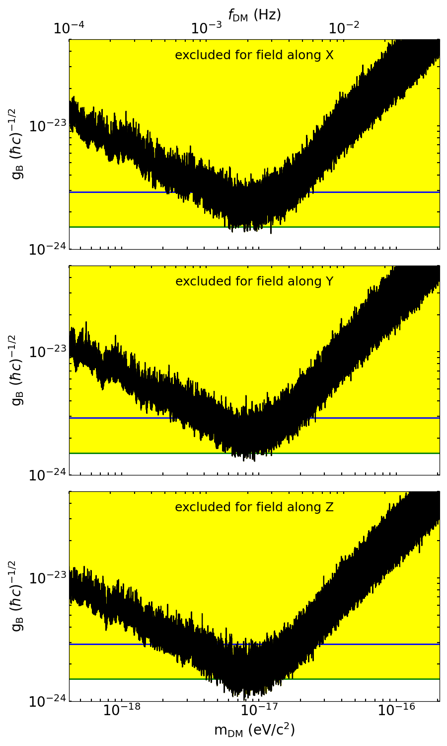
We assumed above that the ULMBs are coupled to B-L. Our constraints on ULMBs coupled to B are shown in Fig. 6. Because $Δ_B ≪Δ_B-L$, our constraints on ULMBs coupled to L are similar to those shown in Fig. 5. In a narrow band of masses around our most sensitive mass $m_DM=8×10^-18$ eV/$c^2$ there is some improvement on the Eöt-Wash EP B limits. MICROSCOPE's result constrains this parameter space.
VI.2 Analysis systematics
We did a variety of tests to verify the accuracy of our analysis. First, we predicted the angle $θ$ in response to a torque signal along $ ^ X $ and added it to the angle data. We ran the entire analysis chain to obtain a resulting amplitude. As shown in Fig. 7, it was consistent with the injected torque amplitude. Fig. 8 shows the response to an injected signal near the resonant frequency of the balance where the frequency-dependent correction outlined in Equation (7) is largest. The most prominent peaks are consistent with the injected signal and demonstrate that the direction of a ULMB signal can be determined. The less prominent peaks occur because of covariance, for example, between $K_Xp(t)e^iω_DMt$ and $K_Yp(t)e^i(ω_DM±2ω_⊕)t$ and $K_Zp(t)e^i(ω_DM±ω_⊕)t$ where $ω_⊕=7.3×10^-5$ rad/s is the sidereal frequency. Since $K_Zp(t)$ is approximately constant, the less prominant peaks are spaced by $ω_⊕$. Previous results with a rotating torsion balance Terrano et~al. 2019 mitigated this by taking data with multiple orientations of the dipole. Fig. 9 shows that the covariance between the science and the daily instrumental basis functions, which could have introduced errors, is negligible.


