Metric topologies over some categories of simple open regions in Euclidean space

Ernest Davis Affiliation: Dept. of Computer Science Affiliation: New York University Email: davise@cs.nyu.edu

Abstract

What does it mean for a shape to change continuously? Over the space of convex regions, there is only one “reasonable” answer. However, over a broader class of regions, such as the class of star-shaped regions, there can be many different “reasonable” definitions of continuous shape change.

We consider the relation between topologies induced by a number of metrics over a number of limited categories of open bounded regions in $\mathbb{E}^{n}$ . Specifically, we consider a homeomorphism-based metric; the Hausdorff metric; the dual-Hausdorff metric; the symmetric difference metric; and the family of Wasserstein metrics; and the topologies that they induce over the space of convex regions; the space of convex regions and unions of two separated convex regions; and the space of star-shaped regions. We demonstrate that:

•

Over the space of convex regions, all five metrics, and indeed any metric that satisfies two general well-behavedness constraints, induce the same topology.
•

Over the space of convex regions and unions of two separated convex regions, these five metrics are all ordered by “strictly finer than” relations. In descending order of fineness, these are: the homeomorphism-based, the dual-Hausdorff, the Hausdorff, the Wasserstein, and the symmetric difference. Also, Wasserstein metrics are strictly ordered among themselves.
•

Over the space of star-shaped regions, the topologies induced by the Hausdorff metric, the symmetric-difference metric, and the Wasserstein metrics are incomparable in terms of fineness.

Keywords: Metric topology, convex regions, star-shaped regions, Hausdorff metric, dual-Hausdorff metric, symmetric-difference metric, Wasserstein metric

1 Introduction

In many applications in physical reasoning and in computer graphics, shapes deform continuously. However, what kinds of functions from time to shapes count as “continuous” depends on the topology of the space of regions; and this, as we will discuss here, is not as clear-cut as one might suppose.

Over the space of points in $\mathbb{E}^{n}$ , there are a number of different metrics in common use: the standard Euclidean distance, the Manhattan distance, and more generally the Minkowski distance with parameter $p$ . But all of these, except the discrete metric, are fundamentally similar, in the sense that they generate the same topology. If a sequence ${\bf x}_{1},{\bf x}_{2}$ converges to $\bf y$ in any of them, then it converges to $\bf y$ in all of them; and if a function $\phi({\bf x})$ is continuous in any of them, it is continuous in all of them.

When one considers the space of regions in $\mathbb{E}^{n}$ , however, the situation is very different. Here, again, there are many different possible natural metrics, with no obvious clear favorite, and these are fundamentally different in the sense that they generate different topologies (Davis 2001; Galton 2000).

For instance, (figure 1) consider the sequence of regions in the plane ${\bf Q}_{1},{\bf Q}_{2}\ldots$ where ${\bf Q}_{i}=((0,1)\times(0,1))\cup((2,2+1/i)\times(0,1))$ . Let ${\bf P}=(0,1)\times(0,1)$ . If one measures the difference between two regions X and Y as the area of their symmetric difference

V({\bf X,Y})=\mbox{area}(({\bf X}\setminus{\bf Y})\>\cup\>({\bf Y}\setminus{\bf X}))

then $V({\bf Q}_{i},{\bf P})=1/i$ , so the sequence ${\bf Q}_{1},{\bf Q}_{2}$ converges to ${\bf P}$ . If one measures it using the Hausdorff distance $H({\bf X},{\bf Y})$ , then $H({\bf Q}_{i},{\bf P})>1$ for all $i$ , so the sequence does not converge to P.

Refer to caption — Figure 1: A sequence of regions that converges in the symmetric-difference metric but not in the Hausdorff metric

In this paper, we consider limited classes of regions and well-known metrics that satisfy two specified well-behavedness conditions. We consider the relations between the topologies that these metrics generate over these classes. We prove results of two general flavors. First, in section 4, we show that, over the space of convex regions there is only one natural metric topology. More precisely, the theorem show that any metric satisfying these well-behavedness conditions generate the same topology. Thus, for instance, there is no way to construct an example analogous to figure 1 using convex regions; if a sequence of convex open regions converges to a convex open region in the area metric, it also converges in the Hausdorff metric, and in any other well-behaved metric over regions.

The second flavor of result, show that, as figure 1 illustrates, if one expands the space of regions under consideration to a broader class of regions, then the different metrics we consider generate different topologies.

Section 1.1 will introduce notational conventions and basic functions. Section 2 will define our two well-behavedness conditions: A well-behaved topology “supports continuous morphing”and “satisfies the region separation condition”. Section 3 defines the metrics we will consider:
A homeomorphism-based metric $M({\bf A,B})$ ;
The Hausdorff metric $H({\bf A,B})$ ;
The dual-Hausdorff metric $H^{d}({\bf A,B})$ ;
The symmetric-difference metric $V({\bf A,B})$ ; and
The family of Wasserstein metrics $W^{\psi}{\bf A,B})$

We demonstrate that:

•

Over the space of convex regions, all five metrics, and indeed any metric that satisfies two general well-behavedness constraints, induce the same topology (section 4).
•

Over the space of convex regions and unions of two separated convex regions, these five metrics are all ordered by “strictly finer than” relations. In descending order of fineness, these are: the homeomorphism-based, the dual-Hausdorff, the Hausdorff, the Wasserstein, and the symmetric difference. Also, Wasserstein metrics are strictly ordered among themselves (section 5).
•

Over the space of star-shaped regions, the topologies induced by the Hausdorff metric, the symmetric difference metric, and the Wasserstein metrics are incomparable in terms of fineness (section 6).

1.1 Notation and basic concepts

$\mathbb{R}$ is the space of real numbers. $\mathbb{E}^{n}$ is $n$ -dimensional Euclidean space. We will generally assume that $n\geq 2$ ; many of our concepts become vacuous or trivial in one-dimensional space, though some carry over.

Real numbers and distances will be notated with italicized variables: $x,d$ .

Points in $\mathbb{E}$ will be notated with boldface lower-case variables: ${\bf p,q}$ . In some of the proofs, it will be convenient to choose an origin and notate points as vectors: $\vec{p},\vec{q}$ . The standard Euclidean distance between points x and y will be denoted $d({\bf p,q})$ .

Subsets of $\mathbb{E}^{n}$ will be notated with boldface capital letters: $\bf P,Q$ .

A region will be a open subset of $\mathbb{E}^{n}$ that is bounded and equal to the interior of its closure (topologically regular). The class of all regions in $\mathbb{E}^{n}$ will be denoted $\mathcal{R}$ (the dimension of the space being left implicit). The closure of A is denoted $\bar{\bf A}$ . The topological boundary of region A (i.e. the closure of A minus A) is denoted @A = $\bar{\bf A}\setminus{\bf A}$ .

The $n$ -dimensional volume of region A is denoted $v({\bf A})$ .

The open ball of radius $d$ centered at point ${\bf p}$ is denoted ${\bf B}({\bf p},d)\subset\mathbb{E}^{n}$ .

The radius of region A at point ${\bf o}\in{\bf A}$ is the radius of the largest spherical open ball that fits inside ${\bf A}$ . The radius (1 argument) of region A is its maximal radius. $\mbox{radius}({\bf A})=\max_{{\bf o}\in{\bf A}}\>\mbox{radius}({\bf A,o})$ .

The diameter of A is the maximal distance between two points in $\bar{\bf A}$ : $\mbox{diameter}({\bf A})=\sup_{{\bf p,q}\in\bar{A}}d({\bf p,q})$ .

The distance from point ${\bf p}$ to region Q is the distance from p to the closest point in the closure of Q.

d({\bf p},{\bf Q})=\min_{{\bf q}\in\bar{\bf Q}}\>d({\bf p,q})

The distance between regions A and B is the smallest distance between points in their closure: $d({\bf A,B})=\min_{{\bf a}\in\bar{\bf A},{\bf b}\in\bar{\bf B}}d({\bf a,b})$ . The distance $d({\bf A,B})$ is not, of course, a metric over regions.

Definition 1

Let P be a region. Let $\delta>0$ .

The dilation of P by $\delta$ is the set of all points within $\delta$ of P.
dilate( ${\bf P},\delta$ ) = $\{{\bf w}\>|\>d({\bf w,P})\leq\delta\}$ .

The erosion of P by $\delta$ is the set of all points more than $\delta$ from the complement of P.
erode( ${\bf P},\delta$ ) = $\{{\bf x}\>|\>d({\bf x,P}^{c})\geq\delta\}$ .

The outer shell of P by $\delta$ , ${\bf O}({\bf P},\delta)=\mbox{dilate}({\bf P},\delta)\setminus{\bf P}$ .

The inner shell of P by $\delta$ , ${\bf I}({\bf P},\delta)={\bf P}\setminus\mbox{erode}({\bf P},\delta)$ .

The regularization of $\bf X\subset\mathbb{E}^{n}$ is the interior of the closure of $\bf X$ . Boolean operators, as applied to regions, are implicitly regularized. For instance if ${\bf P}=(0,1)\times(0,1)$ , ${\bf Q}=(1,2)\times(0,1)$ , and ${\bf R}=(0,2)\times(0,1)$ , then ${\bf P}\cup{\bf Q}={\bf R}$ and ${\bf R}\setminus{\bf Q}={\bf P}$ .

Subsets of $\mathcal{R}$ – that is, sets of subsets of $\mathbb{E}^{n}$ — will be denoted using calligraphic letters: $\mathcal{U}$ , $\mathcal{V}$ .
In particular $\mathcal{C}$ is the set of all convex regions.
${\mathcal{D}}^{2}$ is the set of all regions that are the union of two separated convex regions:
${\mathcal{D}}^{2}=\{{\bf X}\cup{\bf Y}\>|\>{\bf X,Y}\in{\mathcal{C}},d({\bf X,Y})>0)$ .
$\mathcal{D}$ will be the set of all regions that are either a single convex region or the union of two separated convex regions; thus ${\mathcal{D}}={\mathcal{C}}\cup{\mathcal{D}}^{2}$ .
${\mathcal{S}}$ will be the set of all bounded, star-shaped regions.

We will use $\mu:\mbox{$\mathcal{R}$}\times\mbox{$\mathcal{R}$}\mapsto\mathbb{R}$ to represent a generic metric over $\mathcal{R}$ ; that is $\mu({\bf A,B})$ is some measure of the difference between regions $\bf A$ and $\bf B$ that satisfies the standard axioms for metrics. We will use upper-case italic letters for specific metrics, as defined in section 3; for instance, the Hausdorff distance is denoted $H({\bf P},{\bf Q})$ .

Otherwise, the font of function symbols will correspond to the type of the value returned by the function. In particular, the ball of radius $d$ relative to the metric $\mu$ centered at region $\bf P$ is denoted ${\mathcal{B}}_{\mu}({\bf P},d)=\{{\bf Q}\>|\>\mu({\bf P},{\bf Q})<d\}$

Finally $\mbox{$\mathbb{T}$}_{\mu}$ will be the topology generated by metric $\mu$ over $\mathcal{R}$ ; since a topology is a set of open sets, $\mbox{$\mathbb{T}$}_{\mu}$ is a set of sets of subsets of $\mathbb{E}^{n}$ .

Throughout this paper, the phrases “ $\mbox{$\mathbb{T}$}_{\alpha}$ is finer than $\mbox{$\mathbb{T}$}_{\beta}$ ” or “is coarser”, if unqualified, are to be interpreted as a non-strict relation; that is, as “finer than or equal to” or “coarser than or equal to”. When a strict relation is intended, the phrases “strictly finer/coarser” will be used. The phrase “ $\mbox{$\mathbb{T}$}_{\alpha}$ is not finer/coarser than $\mbox{$\mathbb{T}$}_{\beta}$ ” will mean “It is not the case that $\mbox{$\mathbb{T}$}_{\alpha}$ is finer/coarser than $\mbox{$\mathbb{T}$}_{\beta}$ .”

2 Well-behaved topologies

Definition 2

Let $\mathcal{U}$ be a set of regions (a subset of $\mathcal{R}$ ). A history over $\mathcal{U}$ is a function $\phi:[0,1]\mapsto\mathcal{U}$ .

Definition 3

A morphing over $\mathbb{E}^{n}$ is a uniformly continuous function $\psi:[0,1]\times\mathbb{E}^{n}\mapsto\mathbb{E}^{n}$ with the following properties:

a.

$\psi(0,\cdot)$ is the identity over $\mathbb{E}^{n}$
b.

For $t\in[0,1]$ , $\phi(t,\cdot$ ) is a homeomorphism of $\mathbb{E}^{n}$ to itself.

Definition 4

A history $\phi:\mathbb{R}\mapsto\mbox{$\mathcal{R}$}$ corresponds to morphing $\psi$ if $\phi(t)=\psi(t,\phi(0))$ .

Definition 5

A topology $\mathbb{T}$ over a subspace $\mathcal{U}$ of $\mathcal{R}$ supports continuous morphing if every history over $\mathcal{U}$ that corresponds to a morphing is continuous relative to $\mathbb{T}$ .

Intuitively, if you start with a spatial region A and you morph it around continuously relative to the regular spatial topology, then its trajectory as a function of time is continuous in $\mathbb{T}$ . This is an upper bound on the fineness of $\mathbb{T}$ ; the topology cannot be so fine that morphings are discontinuous. If $\mathbb{T}$ supports continuous morphing and $\mbox{$\mathbb{T}$}^{\prime}$ is coarser than $\mathbb{T}$ , then $\mbox{$\mathbb{T}$}^{\prime}$ also supports continuous morphing.

The following is an example of a metric that does not support continuous morphing. Let $\mathcal{U}$ be the set of regions in $\mathbb{E}^{2}$ with a finite perimeter. Define the metric over $\mathcal{U}$ , $\mu({\bf X,Y})=H({\bf X,Y})+|\mbox{perimeter}({\bf X})-\mbox{perimeter}({\bf Y})|$ . Then one can easily define a morphing in which $\phi(0)$ is the unit square and $\phi(t)$ is the unit square with a saw-toothed boundary, where the teeth are at $45^{\circ}$ and the length of the teeth is $t$ . Then for all $t>0$ , the perimeter of $\phi(t)$ is approximately $4\sqrt{2}$ , so the morphing is not continuous relative to $\mbox{$\mathbb{T}$}_{\mu}$ .

Definition 6

A topology $\mathbb{T}$ over $\mathcal{R}$ satisfies the region separation condition if the following hold for any regions ${\bf P,Z}\in\mbox{$\mathcal{R}$}$ :

i.

If ${\bf P}\cap{\bf Z}=\emptyset$ , then in $\mathbb{T}$ there exists a neighborhood $\mathcal{U}$ of $\bf P$ such that no superset of ${\bf Z}$ is in $\mathcal{U}$ .
ii.

If ${\bf P}\supset{\bf Z}$ , then in $\mathbb{T}$ there exists a neighborhood $\mathcal{U}$ of $\bf P$ such that no region that is disjoint from ${\bf Z}$ is in $\mathcal{U}$ .

Lemma 1

Let $\mathbb{T}$ be a topology over $\mathcal{R}$ that satisfies the region separation condition. Let $\phi:\mathbb{R}\mapsto\mbox{$\mathcal{R}$}$ be a history that is continuous under $\mathbb{T}$ . Let ${\bf Z}\in\mbox{$\mathcal{R}$}$ be any open region. Then there exists a neighborhood $U$ of 0 such that

•

if ${\bf Z}\cap\phi(0)=\emptyset$ then there is no $t\in U$ such that ${\bf Z}\subset\phi(t)$ ;
•

if ${\bf Z}\subset\phi(0)$ then there is no $t\in U$ such that ${\bf Z}\cap\phi(t)=\emptyset$ .

Proof: Taking ${\bf P}=\phi(0)$ , construct the set $\mathcal{U}$ to satisfy the conclusion of definition 6. Take $U=\phi^{-1}({\mathcal{U}})$ . By continuity, $U$ is open and by construction it satisfies the conditions of the theorem.

Definition 7

A topology is well-behaved if it supports continuous morphing and satisfies the region separation condition.

It is immediate from the definitions that if a topology supports continuous morphing, then every coarser topology does; and that if a topology satisfies the region separation condition, then every finer topology does.

3 Metrics on the space of regions

In this paper, we primarily consider five metrics, or families of metrics, over the space of regions: a homeomorphism-based metric $M({\bf A,B})$ ; the Hausdorff metric $H({\bf A,B})$ ; the dual-Hausdorff metric $H^{d}({\bf A,B})$ ; the symmetric-difference metric $V({\bf A,B})$ ; and the family of Wasserstein metrics $W^{\psi}({\bf A,B})$

Some other metrics will be discussed in passing at various points.

3.1 Homeomorphism-based metric

There are a number of different ways of defining the difference between two regions A and B in terms of homeomorphisms between them or between their boundaries. Perhaps the oldest and the best known is the Fréchet distance. In this paper we will use the homeomorphism distance $M({\bf A,B})$ , defined as follows:

Let A and B be two regions in $\mathbb{E}^{n}$ . Let $\Gamma({\bf A},{\bf B})$ be the set of all homeomorphisms $\gamma$ of $\mathbb{E}^{n}$ to itself such that $\gamma({\bf A})={\bf B}$ . Define the metric

M({\bf A,B})=\inf_{\gamma\in\Gamma}\sup_{{\bf x}\in\mathbb{E}^{n}}d({\bf x},\gamma({\bf x}))

(If $\Gamma=\emptyset$ — that is, there are no homeomorphisms of the space that map A to B — then $M({\bf A,B})=\infty$ .)

In other words: for any $\gamma$ that is an homeomorphism from $\mathbb{E}^{n}$ to itself and that maps $\bf A$ to $\bf B$ , we define a cost which is the maximum distance from $\bf x$ to $\gamma({\bf x})$ for any $\bf x$ in $\mathbb{E}^{n}$ We then define the metric $M({\bf A,B})$ as the smallest cost attained by any such $\gamma$ (more precisely, the infimum).

Theorem 1

The topology $\mbox{$\mathbb{T}$}_{M}$ supports continuous morphings over $\mathcal{R}$ .

Proof: Immediate from the definition.

A converse of theorem 1 would be the claim that if a history is continuous relative to $\mbox{$\mathbb{T}$}_{M}$ then it corresponds to a morphing. I suspect that this is true, but have not been able to prove it.

3.2 The Hausdorff and dual-Hausdorff metrics

The one-sided Hausdorff distance from region P to Q is the supremum over points p in P of the distance from p to Q.

H^{1}({\bf P,Q})=\sup_{{\bf p}\in{\bf P}}d({\bf p,Q})

The Hausdorff distance between regions and P to Q is the maximum of (the one-sided Hausdorff distance from P to Q) and (the one-sided Hausdorff distance from Q to P)

H({\bf P,Q})=\max(H^{1}({\bf P,Q}),H^{1}({\bf Q,P}))

The dual-Hausdorff distancei (Davis 1995) is the maximum of (the Hausdorff distance between P and Q) and (the Hausdorff distance between the complements of P and Q).

H^{d}({\bf P,Q})=\max(H({\bf P,Q}),H({\bf Q}^{c},{\bf P}^{c}))

This metric is not discussed in (Deza and Deza 2006) but the proof that it is a metric over the space of regular regions is immediate.

It is immediate from the definitions that for all regions, $H({\bf P,Q})\leq H^{d}({\bf P,Q})\leq M({\bf P,Q})$ and therefore $\mbox{$\mathbb{T}$}_{M}$ is finer than $\mbox{$\mathbb{T}$}_{H^{d}}$ which is finer than $\mbox{$\mathbb{T}$}_{H}$ .

Theorem 2

Topologies $\mbox{$\mathbb{T}$}_{H^{d}}$ and $\mbox{$\mathbb{T}$}_{H}$ support continuous morphing over $\mathcal{R}$ .

Proof: Immediate from theorem 1 together with the above.

Theorem 3

The Hausdorff distance has the region separation property over $\mathcal{R}$ .

Proof: i. Let P, Z be regions such that ${\bf P}\cap{\bf Z}=\emptyset$ . Let ${\bf Y}\supset{\bf Z}$ . Let z be a point in Z. Then $H({\bf Y,P})\geq d({\bf z,P})$ . So for $\epsilon<d({\bf z,P})$ , the open ball ${\mathcal{B}}_{H}({\bf P},\epsilon)$ excludes all Z and any superset of Z.

ii. Let P, Z be regions such that ${\bf Z}\subset{\bf P}$ . Let Y be a region such that ${\bf Z}$ and Y are disjoint. Let z be a point in Z. Then $H({\bf Y,P})\geq\mbox{radius}({\bf P,z})$ . So for $\epsilon<\mbox{radius}({\bf Z,z})$ , the open ball ${\mathcal{B}}_{H}({\bf P},\epsilon)$ excludes all Y and any subset of Y.

Corollary 2

The metrics $M({\bf P,Q})$ and $H^{d}({\bf P,Q})$ have the region separation property over $\mathcal{R}$ .

Proof: It is immediate that, if a topology has the property, then any finer topology also has the property.

3.3 The symmetric-difference metric

Define the function S(P,Q): $\mbox{$\mathcal{R}$}\times\mbox{$\mathcal{R}$}\mapsto\mbox{$\mathcal{R}$}$ as the symmetric difference of regions P and Q:
${\bf S(P,Q)}=({\bf P}\setminus{\bf Q})\cup({\bf Q}\setminus{\bf P})$

The symmetric-difference metric is the $n$ -dimensional measure of the symmetric difference:
$V({\bf P,Q})=v({\bf S(P,Q}))$

Theorem 4

Over the space $\mathcal{R}$ , $\mbox{$\mathbb{T}$}_{H^{d}}$ is finer than $\mbox{$\mathbb{T}$}_{V}$ .

Proof: See (Davis 2001), corollary 8.2.

Theorem 5

$\mbox{$\mathbb{T}$}_{V}$ supports continuous morphings over $\mathcal{R}$ .

Proof: Immediate from theorem 2 and lemma 4.

Theorem 6

$\mbox{$\mathbb{T}$}_{V}$ has the region separation property over $\mathcal{R}$ .

Proof:
i. Let P, Z be regions such that ${\bf P}\cap{\bf Z}=\emptyset$ . Let ${\bf Y}\supset{\bf Z}$ . Then ${\bf Z}\subset S({\bf P,Y})$ , $V({\bf P,Y})\geq v({\bf Z})$ . So for $\epsilon<v({\bf Z})$ , the open ball ${\mathcal{B}}({\bf P},\epsilon)$ excludes Z and any superset of Z.

ii. Let P,Z be regions such that ${\bf Z}\subset{\bf P}$ . Let Y be a region such that ${\bf Z}$ and Y are disjoint. Then again ${\bf Z}\subset S({\bf P,Y})$ , So for $\epsilon<v({\bf Z})$ , the open ball ${\mathcal{B}}({\bf P},\epsilon)$ excludes all sets disjoint from Z.

3.4 Wasserstein metrics

The family of Wasserstein distances $W^{\psi}({\bf P,Q})$ are generalizations of the “earth-movers” metric often used in comparing probability distributions.

Definition A function $\psi:\mathbb{R}^{\geq 0}\mapsto\mathbb{R}^{\geq 0}$ is a Mulholland function if it is continuous and monotonically increasing; $\psi(0)=0$ ; $\lim_{x\mbox{$\rightarrow$}\infty}\psi(x)=\infty$ ; and $\psi$ satisifies the Mulholland (1949) inequality

\psi^{-1}(\sum_{i=1}^{n}\psi(x_{i}+y_{i}))\leq\psi^{-1}(\sum_{i=1}^{n}\psi(x_{i}))+\psi^{-1}(\sum_{i=1}^{n}\psi(y_{i}))

The Minkowski inequality is the special case where $\phi(x)=x^{p}$ .

The Wasserstein distance corresponding to a Mulholland function $\psi$ is a metric over probability distributions. (It is usually defined using the particular function $\psi(x)=x^{p}$ . However, since the only property of $x^{p}$ that is used in proving that the Wasserstein distance is a metric is that it satisfies the Mulholland inequality, one can generalize it to use any Mulholland function (Clement and Desch, 2008).)

Definition 8

Let $\psi$ be a Mulholland function. Let $\theta({\bf x})$ and $\zeta({\bf x})$ be probability densities over $\mathbb{E}^{n}$ . Let $\gamma$ be a function from $\mathbb{E}^{n}$ to $\mathbb{E}^{n}$ such that, if random variable $X$ has density $\theta({\bf x})$ then $\gamma(X)$ will have density $\zeta({\bf x})$ . Define the integral

I(\gamma)=\int_{{\bf x}\in\mathbb{E}^{n}}\theta({\bf x})\cdot\psi(d({\bf x},\gamma({\bf x})))\>d{\bf x}

Let $\Gamma(\theta,\zeta)$ be the set of all such $\gamma$ . Then the Wasserstein distance between $\theta$ and $\zeta$ corresponding to $\psi$ is defined as follows:

W^{\psi}(\theta,\zeta)=\inf_{\gamma\in\Gamma(\theta,\zeta)}\psi^{-1}(I(\gamma))

We adapt the above definition to be a distance between regions ${\bf P}$ and ${\bf Q}$ by taking $\theta$ and $\zeta$ to be the uniform distributions over ${\bf P}$ and ${\bf Q}$ .

Definition 9

For any region P, $U_{\bf P}$ represents the uniform distribution over P:
$U_{\bf P}({\bf x})=1/v({\bf P})$ for ${\bf x}\in{\bf P}$ .
$U_{\bf P}({\bf x})=0$ for ${\bf x}\not\in{\bf P}$ .

Definition 10

Let P and Q be regions in $\mathcal{R}$ . Let $\psi$ be a Mulholland function. Define $W^{\psi}({\bf P,Q})$ to be $W^{\psi}(U_{\bf P},U_{\bf Q})$

We can reformulate this definition as follows:

Definition 11

Let $\bf P$ and $\bf Q$ be regions. Let $\gamma$ be a function from P to Q. We say that $\gamma$ is uniform if, for all ${\bf X}\subset{\bf P}$ , $v(\gamma({\bf X})))=v({\bf X})\cdot v({\bf Q})/v({\bf P})$ . That is, $\gamma$ preserves relative measure.

Define the following two functions of $\gamma$ and ${\bf P}$ :

I^{\psi}(\gamma,{\bf P})=\frac{1}{v({\bf P})}\cdot\int_{{\bf x}\in P}\psi(d({\bf x},\gamma({\bf x})))\>\mbox{d}{\bf x}

C^{\psi}(\gamma,{\bf P})=\psi^{-1}(I^{\psi}(\gamma,{\bf P}))

Let $\Gamma({\bf P,Q})$ be the set of all uniform functions $\gamma$ from P to Q. Then $W^{\psi}({\bf P,Q})=\inf_{\gamma\in\Gamma({\bf P,Q})}C^{\psi}({\bf P,Q})$ .

In the case of the identity function $\psi(x)=x$ , this can be given an intuitive motivation as follows: Suppose that you have dirt uniformly spread over $\bf P$ and you want to move it so that it is uniformly spread out over $\bf Q$ . To move a small piece of dirt of mass $m$ from x to y will cost $m\cdot d({\bf x,y})$ . Then if you follow $\gamma$ as a guide for how to move the dirt, the total cost will be $C^{\psi}(\gamma)$ . Thus the cost of the cheapest way of moving the dirt is $W^{\psi}({\bf A,B})$ . Hence this is known as the “earth-mover’s” metric.

Lemma 3

Let P be a bounded region; let $W^{\psi}$ be a Wasserstein metric; let $\zeta$ and $\theta$ be probability distributions that are zero outside P. Let $p=$ diameter(P). Let $m=\int_{{\bf x}\in\bf P}\max(0,\zeta(x)-\theta(x))\>dx$ Then $W^{\psi}(\zeta,\theta)\leq\psi^{-1}(m\cdot\psi(p))$ .

Informal proof: The amount of “dirt” that has to be moved in turning $\zeta$ into $\theta$ is
$\int_{{\bf x}\in\bf P}\max(0,\zeta({\bf x})-\theta({\bf x})|\>d{\bf x}$ . The distance that any piece of dirt can be moved is at most $p$ . So for any $\gamma$ that turns $\theta$ into $\phi$ , $I^{\psi}(\gamma,{\bf P})\leq m\cdot\psi(p)$ . Then $W^{\psi}(\psi,\theta)\leq\psi^{-1}(I^{\psi}(\gamma,{\bf P})=\psi^{-1}(m\cdot\psi(p))$ .

Lemma 4

Let ${\bf P,Q}$ be regions. Let $p$ =diameter(P), $h=H({\bf P,Q})$ , and $a=V({\bf P,Q})$ . Assume that $a<v({\bf P})/2$ and that $h<p/2$ . Let $\psi$ be a Mulholland function. Then $W^{\psi}({\bf P,Q})\leq\psi^{-1}(4a\psi(p)/v({\bf P}))$ .

Proof: Let $\zeta=U_{\bf P}$ and $\theta=U_{\bf Q}$ . Let ${\bf R}={\bf P}\cup{\bf Q}$ ; thus $\zeta$ and $\theta$ are zero outside $\bf R$ .

Note that $v({\bf P})+a\geq v({\bf Q})\geq v({\bf P})-a\geq v({\bf P})/2$
so $|1/(v({\bf P})-1/v({\bf Q}))|=|v({\bf Q})-v({\bf P})|/(v({\bf P})v({\bf Q}))\leq a/2v^{2}({\bf P})$ .

\int_{{\bf x}\in\bf R}\max(\zeta({\bf x})-\theta({\bf x}),0)\>dx=\int_{{\bf x}\in{\bf P}\cap{\bf Q}}\max(\zeta({\bf x})-\theta({\bf x}),0)\>dx+\int_{{\bf x}\in{\bf S}({\bf P},{\bf Q})}\max(\zeta({\bf x})-\theta({\bf x}),0)\>dx

But in the first integral in the sum, the volume of the region of integration is at most $v({\bf P})$ and the integrand is at most $|1/v({\bf Q})-1/v({\bf P})|$ so the value of the integral is at most $2a/v({\bf P})$ .

In the second integral, the volume of integration is ${\bf S}({\bf P,Q})$ and the integrand is at most $1/\min(v({\bf P}),v({\bf Q}))$ so value of the integral is at most $2a/v({\bf P})$ .

Thus

\int_{{\bf x}\in\bf R}\max(\zeta({\bf x})-\theta({\bf x}),0)\>dx\leq 4a/v({\bf P})

Using lemma 3 it follows that $W^{\psi}({\bf P,Q})\leq\psi^{-1}(4a\psi(p)/v({\bf P}))$ .

Theorem 7

For any Mulholland function $\psi$ , the topology generated by Wasserstein distance $\mbox{$\mathbb{T}$}_{W^{\psi}}$ is coarser over $\mathcal{R}$ than the topology generated by the dual-Hausdorff distance $\mbox{$\mathbb{T}$}_{H^{d}}$

Proof: Choose region P and $\epsilon>0$ . Let $p$ =diameter(P). Let $b=\psi(\epsilon)v({\bf P})/4\psi(p)$ . Using theorem 4, choose $\delta_{1}$ such that, such that, for all regions $\bf Q$ , if $H^{d}<\delta_{1}$ then $V({\bf P,Q})<b$ . Let $\delta=\min(\delta_{1},p/2)$ . Then by lemma 4 it follows that $W^{\psi}({\bf P,Q})<\epsilon$ .

Corollary 5

For any Mulholland function $\psi$ , the Wasserstein distance $W^{\psi}$ supports continuous morphing over $\mathcal{R}$ .

Proof: Immediate from theorems 7 and 2.

Theorem 8

For any Mulholland function $\psi$ , the Wasserstein distance $W^{\psi}$ satisfies the region separation condition over $\mathcal{R}$ .

Proof:

Part 1: Let ${\bf P,Z}$ be regions such that $d({\bf P,Z})>0$ . Let $c=d({\bf P,Z})/2$ . Let ${\bf Q}=\mbox{dilate}({\bf P},c)$ . Let Y be any superset of Z. The part of Y that is more than $c$ from $\bf P$ includes at least $\bf Z$ ; the part Y that is less than $c$ from $\bf P$ is a subset of $\bf Q$ . So the fraction of Y that is more than $c$ from P is at least $v({\bf Z})/(v({\bf Z})+v({\bf Q})$ . So, for any uniform function $\gamma$ from P to Y, $I^{\psi}({\bf P},\gamma)\geq(v({\bf Z})/(v({\bf Z})+v({\bf Q}))\cdot\psi(c)$ , so there is a positive lower bound on $W^{\alpha}({\bf P,Y})$ .

The proof of Part 2 is analogous.

4 The topology of the space of bounded convex open regions

We show that there is a unique well-behaved topology over the space of convex regions. Since all of the metric topologies we consider are well-behaved over that space, it follows that they all generate the same topology.

Shephard and Webster (1995) demonstrated that the Hausdorff metric and the symmetric-difference metric generate identical topologies over the space of convex regions; that two further metrics, which they named the “difference body metric” and the “homogeneous symmetric difference” likewise generate the same topology. The latter two results are subsumed in theorem 9 below, though we do not prove that here. Groemer (2000) gives strong bounds between the relative size of the Hausdorff distance and the symmetric-difference distance between two convex regions.

Lemma 6

Let $\bf A$ be a bounded open, convex region in $\mathbb{E}^{n}$ . Let ${\bf p}\in\bf A$ , and let ${\bf q}\in@{\bf A}$ . For $t\geq 0$ , let ${\bf w}(t)={\bf q}+t({\bf q}-{\bf p})$ . Then, for $t\geq 0$ , the function $f(t)=d({\bf w}(t),@{\bf A})$ is an increasing function of $t$ .

Proof: (Figure 2). Let $0<t_{1}<t_{2}$ . Let $\bf b$ be the point on $@{\bf A}$ closest to ${\bf w}(t_{2})$ . Let $L$ be the line from p to $\bf b$ . Since $\bf A$ is convex, the portion of $L$ between $\bf b$ and ${\bf p}$ is entirely in $\bf A$ . Let $M$ be the line through ${\bf w}(t_{1})$ parallel to the line ${\bf bw}(t_{2})$ and let $\bf c$ be the intersection of $L$ and $M$ . Then the triangle $\bigtriangleup{\bf q},{\bf w}(t_{1}),{\bf c}$ is similar to the triangle $\bigtriangleup{\bf q},{\bf w}(t_{2}),{\bf b}$ and lies inside it. Hence

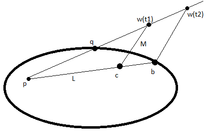
f(t_{1})=d({\bf w}(t_{1}),{\bf A})\leq d({\bf w}(t_{1}),{\bf c})<d({\bf w}(t_{2}),{\bf b})=f(t_{2})

Lemma 7

Let $\bf P$ and $\bf Q$ be bounded, convex, open sets, and let o be a point in P. Let $h=H({\bf P,Q})$ and $r=\mbox{radius}({\bf P,o})$ . If $h<r$ then ${\bf B}({\bf o},r-h)\subset{\bf Q}$ .

Proof: For convenience, take $\vec{0}={\bf o}$ . Let $\vec{x}$ be a point in ${\bf B}(\vec{0},r)\setminus{\bf Q}$ (If there is no such point, the conclusion is trivial.) Then there is a hyperplane $\bf X$ through $\vec{x}$ such that ${\bf Q}$ lies on one side of $\bf X$ . Let ${\bf C}$ be the intersection of X with ${\bf B}(\vec{0},r)$ . ( $\bf C$ is an $n-1$ -dimensional solid circular disk). Let $\vec{c}$ be the center of ${\bf C}$ ; thus $\vec{c}$ is the closest point to $\vec{0}$ on $\bf C$ , so $|\vec{c}|\leq|\vec{x}|$ .

Q must lie in the side of X that contains $\vec{0}$ ; if it lies on the far side of X, then its distance from the point in ${\bf B}(\vec{0},r)$ opposite $\vec{c}$ would be greater than $r$ , which is impossible.

Let $\vec{y}=r\cdot\vec{c}/|\vec{c}|$ . Then $\vec{c}$ is the closest point on ${\bf B}(\vec{0},r)$ to $\vec{y}$ . In particular $d(\vec{y},\vec{c})\leq d(\vec{y},{\bf Q})\leq h$ . But $d(\vec{y},\vec{c})=r-|\vec{c}|\geq r-|\vec{x}|$ so $|\vec{x}|\geq r-h$ , so $\vec{x}\not\in{\bf B}(\vec{0},r-h)$ . (Figure 3)

Definition 12

Let ${\bf P,Q,W}$ be open convex bounded regions such that ${\bf P}\cap{\bf Q}\neq\emptyset$ , $\bar{\bf P}\subset{\bf W}$ and $\bar{\bf Q}\subset{\bf W}$ . That is, P and Q overlap, and W contains them both, with some separation between ${\bf P}\cup{\bf Q}$ and the outside of W (figure 4).

Let o be a point in ${\bf P}\cap{\bf Q}$ .

For convenience, let $\vec{0}=\bf o$ and $\vec{x}={\bf x}-{\bf o}$ . For any unit vector $\hat{v}$ , let ${\bf R}(\hat{v})$ be the ray $\{t\hat{v}\>|\>t\in(0,\infty)\}$ . Let $\vec{p}(\hat{v})$ , $\vec{q}(\hat{v})$ , $\vec{w}(\hat{v})$ be the intersections of ${\bf R}(\hat{v})$ with $@{\bf P}$ , $@\bf Q$ , and $@{\bf W}$ respectively. Since P, Q and W are convex, it is immediate that $\vec{p}(\hat{v})$ and $\vec{q}(\hat{v})$ and $\vec{w}(\hat{x})$ are uniquely defined (in any direction $\hat{v}$ there is only one such intersection for each) and are continuous functions of $\hat{v}$ .

The standard morphing of P into Q within W centered at o, denoted $\Gamma_{\bf P,Q,W,o}:[0,1]\times\mathbb{E}^{n}\mapsto\mathbb{E}^{n}$ is defined as the following function:

For all $t\in[0,1]$ , $\Gamma_{\bf P,Q,W,o}(t,\vec{0})=\vec{0}$ .

For $\vec{x}\neq\vec{0}$ , let $\hat{x}=\vec{x}/|\vec{x}|$ . To simplify the expression, fix a direction of $\hat{x}$ , and let $x=|\vec{x}|$ . $p=|\vec{p}(\hat{x})|$ , $q=|\vec{q}(\hat{x})|$ , and $w=|\vec{w}(\hat{x})|$ . Then, for any $\vec{x}$ in the ray ${\bf R}(\hat{x})$ ,

•

If $x\leq p$ , then $\Gamma(t,\vec{x})=((1-t)x+t(xq/p))\cdot\hat{x}$ .

•

If $p<x<w$ , then $\Gamma(t,\vec{x})=((1-t)x+t(q+(w-q)(x-p)/(w-p)))\cdot\hat{x}$ .

•

If $w\leq x$ , then $\Gamma(t,\vec{x})=\vec{x}$ .

Thus, each ray ${\bf R}(\hat{x})$ is divided into three parts: the part inside P, the part between part P and W, and the part outside W. $\Gamma$ is a transformation, piecewise bilinear in both $t$ and $x$ , which transforms the first part into the part of the ray inside $\bf Q$ , the second part into the part of the ray between $\bf Q$ and $\bf W$ , and is the identity outside $\bf W$ .

Lemma 8

Let $\bf P,Q,W,o$ be as in definition 12. Let $h=H({\bf P,Q})$ , $r$ = radius(P,o), and $a=\mbox{diameter}({\bf P})$ . If $r>h$ , then the standard morphing $\Gamma_{\bf P,Q,W,o}$ has the following properties:

a.

$\Gamma$ is a continuous morphing.
b.

for all ${\bf x}\in\mathbb{E}^{n}$ , $\Gamma(0,{\bf x})={\bf x}$ .
c.

for all $t\in[0,1]$ and ${\bf x}\not\in{\bf W}$ , $\Gamma(t,{\bf x})={\bf x}$ .
d.

$\Gamma(1,{\bf P})={\bf Q}$ ;
e.

for all $t\in[0,1]$ , $H(\Gamma(t,{\bf P}),{\bf P})\leq h$ ; and
f.

for all ${\bf x}\in\mathbb{E}^{n}$ and $t\in[0,1]$ , $d(\Gamma(t,{\bf x}),{\bf x})\leq d({\bf x,o})\cdot ah/(r-h)$ .

Proof:

Properties (a), (b), and (c) are immediate by construction.

Let $\vec{0}=\bf o$ ; $\vec{x}={\bf x}-{\bf o}$ and define $\hat{x}$ , $\vec{p}(\hat{x})$ , and $\vec{q}(\hat{x})$ as in definition 12.

For (d): for any point $\vec{p}(\hat{v})\in@{\bf P}$ , $\Gamma(0,\vec{p}(\hat{v}))=\vec{p}(\hat{v})$ and $\Gamma(1,\vec{p}(\hat{v}))=\vec{q}(\hat{v})$ . Since P and Q are convex, it follows that $\Gamma(1,@{\bf P})=@{\bf Q}$ and therefore $\Gamma(1,{\bf P})={\bf Q}$ .

Condition (e) of the lemma asserts that, for all $t$ , $H({\bf P},\Gamma(t,{\bf P}))\leq H({\bf P},{\bf Q})$ ; that is for all $\vec{x}\in\Gamma(t,{\bf P})$ , $d(\vec{x},{\bf P})\leq h$ and for all $\vec{x}\in{\bf P}$ , $d(\vec{x},\Gamma(t,{\bf P}))\leq h$

To prove this, let $\vec{x}$ be a point in $\Gamma(t,{\bf P})$ , and let $\hat{x}=\vec{x}/|\vec{x}|$ . Then the points $\vec{0},\vec{x},\vec{p}(\hat{x})$ , and $\vec{q}(\hat{x})$ are collinear. If $|\vec{x}|<|\vec{p}(\hat{x})|$ then $\vec{x}\in{\bf P}$ , so $d(\vec{x},{\bf P})=0$ . If $|\vec{x}|\geq|\vec{p}(\hat{x})|$ then $|\vec{q}(\hat{x})|>|\vec{p}(\hat{x})|$ and $\vec{x}$ is on the line between $\vec{p}(\hat{x})$ and $\vec{q}(\hat{x})$ so, by lemma 6, $d(\vec{x},{\bf P})\leq d(\vec{q}(\hat{x}),{\bf P})\leq H({\bf Q},{\bf P})$ .

Now let $\vec{x}$ be a point in $\bf P$ , and let $\hat{x}=\vec{x}/|\vec{x}|$ . If $\vec{x}\in\Gamma(t,{\bf P})$ then $d(\vec{x},f(t,{\bf P}))=0$ . If $\vec{x}\not\in\Gamma(t,{\bf P})$ then $\vec{x}$ must be on the line through $\vec{q}(\hat{x})$ and $\vec{p}(\hat{x})$ with $|\vec{q}(\hat{x})|<|\vec{x}|<\vec{p}(\hat{x})$ . By lemma 6 $d(\vec{x},{\bf Q})\leq d(\vec{p}(\hat{x}),{\bf Q})\leq H({\bf Q},{\bf P})$ .

Condition (f) of the lemma asserts that for all $\vec{x}\in\mathbb{E}^{n}$ and $t\in[0,1]$ , $d(\Gamma(t,\vec{x}),\vec{x})\leq ph/(r-h)$ . By construction, the point on the ray $\{t\hat{x}|t>0\}$ that is moved furthest is $\vec{p}(\hat{x})$ , so it suffices to prove the inequality for that point.

Since

\Gamma(t,\vec{x})=\vec{x}\cdot(1+\frac{t\cdot(|\vec{q}(\hat{x}|-|\vec{p}(\hat{x}|}{|\vec{p}(\hat{x})|})

we have

d(\Gamma(t,\vec{x}),\vec{x})=|\vec{x}|\cdot t\frac{\mbox{abs}(|\vec{q}(\hat{x}|-|\vec{p}(\hat{x}|)}{|\vec{p}(\hat{x})|}

Our goal, then, is to bound the above fraction as a function of $r$ and $h$ . For convenience since $\hat{x}$ will be fixed, we will drop the argument and just write $\vec{p}$ and $\vec{q}$ .

Consider first the case where $|\vec{q}|<|\vec{p}|$ . The ray ${\bf R}=\{t\hat{x}|t\in(0,\infty)\}$ is thus divided into three parts: the segment from $\vec{0}$ to $\vec{q}$ is in both Q and P; the segment from $\vec{q}$ to $\vec{p}$ is in ${\bf P}$ but not $\bf Q$ ; and the segment past $\vec{p}$ is in neither. By lemma 7, the ball ${\bf B}(\vec{0},r-h)\subset{\bf Q}$ . Construct the cone $\bf C$ with apex $\vec{q}$ that is tangent to ${\bf B}(\vec{0},r-h)$ (figure 5). Since $\bf Q$ is convex, ${\bf C}\subset{\bf Q}$ . Let $\bf C^{\prime}$ be the reflection of C through $\vec{q}$ . Then $\bf C^{\prime}$ must be disjoint from $\bf Q$ . (For any point $\vec{w}\in{\bf C^{\prime}}$ there are points $\vec{v}$ on the part of the ray R past $\vec{q}$ and $\vec{u}\in{\bf C}$ such that $\vec{u},\vec{v},\vec{w}$ are collinear in that order; since $\bf Q$ is convex, $\vec{u}\in{\bf Q}$ and $\vec{v}\not\in\bf Q$ , it follows that $\vec{w}\not\in{\bf Q}$ .)

Construct the sphere centered at $\vec{p}$ tangent to ${\bf C}^{\prime}$ . Let $z$ be the radius of the sphere. Since ${\bf p}\in@{\bf P}$ and the sphere is disjoint from $\bf Q$ , we have $h\geq z$ .

Now let $\vec{a}$ be a point in $\bar{\bf B}(\vec{0},(r-h))\cap{\bf C}$ and let $\vec{b}$ be a point in $\bar{\bf B}(\vec{p},z)\cap{\bf C}^{\prime}$ such that $\vec{a},\vec{q},\vec{b}$ are collinear. Then the triangles $\bigtriangleup\vec{0},\vec{a},\vec{q}$ and $\bigtriangleup\vec{p},\vec{b},\vec{q}$ are similar right triangles. So $d(\vec{0},\vec{a})/d(\vec{0},\vec{q})=(r-h)/|\vec{p}|=d(\vec{p},\vec{b})/d(\vec{p},\vec{q})=z/(|\vec{p}|-|\vec{q}|)$ .

Combining these and rearranging we get $(|\vec{p}|-|\vec{q}|)/|\vec{p}|\leq h/(r-h)$ .

In the case where $|\vec{p}|<|\vec{q}|$ , the analysis is exactly analogous, except that in that case you get the tighter bound $(|\vec{p}|-|\vec{q}|)/|\vec{p}|\leq h/r$ .

Corollary 9

Let ${\bf P,Q}$ be convex regions such that ${\bf P}\cap{\bf Q}\neq\emptyset$ . Let $h=H({\bf P,Q})$ , $r$ = radius(P,o), and $a=\mbox{diameter}({\bf P})$ . Then there is a homeomorphism $g$ of $\mathbb{E}^{n}$ to itself such that $g({\bf P})={\bf Q}$ and, for all ${\bf x}\in{\bf P}$ , $d({\bf x},g({\bf x}))\leq ah/(r-h)$ .

Proof: Find a convex region ${\bf w}\supset{\bf P}\cup{\bf Q}$ and choose a point ${\bf o}\in{\bf P}\cap{\bf Q}$ . Then by lemma 8 the function $\Gamma_{\bf P,Q,W,o}(1,\cdot)$ satisfies the condition of the corollary.

It seems likely that this bound can be substantially tightened using a different morphing and in particular that the dependence on diameter(P) can be eliminated. But for the purposes of our analysis, this will suffice.

Lemma 10

Let $\mathbb{T}$ be a topology over $\mathcal{R}$ that supports continuous morphing. Then, restricted to $\mathcal{C}$ , $\mbox{$\mathbb{T}$}_{H}$ , the topology induced by the Hausdorff metric, is at least as fine as $\mathbb{T}$ .

Proof of the contrapositive: Suppose that $\mbox{$\mathbb{T}$}_{H}$ is not a refinement of $\mathbb{T}$ . Then there exists a region ${\bf P}\in\mbox{$\mathcal{C}$}$ and a sequence of regions ${\bf Q}_{1},{\bf Q}_{2}\ldots\in\mbox{$\mathcal{C}$}$ that converges to ${\bf P}$ in $\mbox{$\mathbb{T}$}_{H}$ but not in $\mathbb{T}$ . Let $r=\mbox{radius}({\bf P})>0$ . Let $\epsilon_{i}=H({\bf Q}_{i},{\bf P})$ ; thus $\lim_{i\mbox{$\rightarrow$}\infty}\epsilon_{i}=0.$ By renumbering we can assume that $\epsilon_{i}<r/2$ for all $i$ .

We are going to use lemma 8 to interpolate a continuous morphing $\phi$ that passes through the regions ${\bf Q}_{1},{\bf Q}_{2},{\bf Q}_{3}\ldots{\bf P}$ at times 1, 1/2, 1/3 …0.

Fix a center point ${\bf o}\in{\bf P}$ . By lemma 7, ${\bf B}({\bf o},r/2)\subset{\bf B}({\bf o},r-H({\bf Q}_{i},{\bf P}))\subset{\bf Q}_{i}$ .

Let $q=1+\mbox{diameter}({\bf P})+\max_{i}H({\bf Q}_{i},{\bf P})$ ; then it is easily shown that the sphere ${\bf R}={\bf B}({\bf o},q)$ contains $\bar{\bf P}$ and $\bar{\bf Q}_{i}$ for all $i$ .

Define the function $f_{k}=\Gamma_{{\bf Q}_{k},{\bf Q}_{k+1},{\bf R},{\bf o}}$ as in definition 12. By lemma 8, $f_{k}(t,{\bf x})$ is a continuous morphing, $f_{k}(0,\cdot)$ is the identity, and $f_{k}(1,{\bf Q}_{i})={\bf Q}_{i+1}$ .
Define the function $g_{k}(t,{\bf x})=f_{k}(k+1-k(k+1)t,{\bf x})$ ; thus $g_{k}(1/k,{\bf x})=f_{k}(0,{\bf x})$ and $g_{k}(1/(k+1),{\bf x})=f_{k}(1,{\bf x})$ .

Now define the function $\phi:\mathbb{R}\times\mathbb{E}^{n}\mapsto\mathbb{E}^{n}$ as follows:

•

Construct $f_{0}$ to satisfy lemma 8 for P and Q. For $t\geq 1$ , define $\phi(t,{\bf x)}=f_{0}(1,{\bf x})$ .
•

For $k=1,2,3\ldots$ , for $t\in[1/(k+1),1/k)$ define $\phi(t,{\bf x})=g_{k}(t,(\phi(1/k,{\bf x}))$
•

for $t\leq 0$ , $\phi(t,\cdot)$ is the identity function on $\mathbb{E}^{n}$

Note that $\phi(1,{\bf P})=f_{0}(1,{\bf P})={\bf Q}_{0}$ .
$\phi(1/2,{\bf P})=g_{1}(1/2,\phi(1,{\bf P}))=f_{1}(1,Q_{0})={\bf Q}_{1}$ .
$\phi(1/3,{\bf P})=g_{2}(1/3,\phi(1/2,{\bf P}))=f_{2}(1,Q_{1})={\bf Q}_{2}$ .
and in general $\phi(1/k,{\bf P})={\bf Q}_{k}$ .

To show that $\phi$ is continuous: Spatial continuity is immediate by construction. Temporal continuity between times of the form $1/k$ is guaranteed by the continuity of $f_{k}$ . Continuity at times of the form $1/k$ follows from the fact that $\phi(t,\cdot)$ consists in expansion along rays emanating from a fixed center point $\vec{0}$ and that the limit at time $t=1/k$ , both from above and below, of the amount of expansion at point $\vec{x}$ is $|\vec{q}_{k}(\hat{x})|/|\vec{p}(\hat{x})|$ , in the notation of lemma 8, where $\vec{q}_{k}(\hat{x})$ is the intersection of ${\bf Q}_{k}$ with the ray $\{t\cdot\hat{x}\>|\>t>0\}$ .

The continuity of $\phi$ at time $t=0$ , which is, of course, the critical point, is guaranteed by the facts that, by lemma 8, for all $t\in[1/(k+1),1/k]$ , $d(\phi(t,\vec{x}),\phi(1/(k+1),\vec{x})\leq 2H({\bf Q}_{k},{\bf Q}_{k+1})/r$ , and that $d(\phi(1/(k+1),\vec{x}),\phi(0,\vec{x})\leq 2H({\bf Q}_{k},{\bf P})/r$ , and by assumption, both of these Hausdorff distances go to zero as $k\mbox{$\rightarrow$}\infty$ .

Lemma 11

Let $\bf P$ be a bounded open region and let ${\bf Q}_{1},{\bf Q}_{2}\ldots$ be an infinite sequence of convex, open regions. Then one of three things is true.

1.

$\lim_{i\mbox{$\rightarrow$}\infty}H({\bf P,Q}_{i})=0$ .
2.

There is a region $\bf Z$ such that ${\bf Z}\subset{\bf P}$ and, for infinitely many ${\bf Q}_{i}$ , ${\bf Z}\cap{\bf Q}_{i}=\emptyset$ .
3.

There is a region $\bf Z$ such that ${\bf Z}\cap{\bf P}=\emptyset$ and, for infinitely many ${\bf Q}_{i}$ , ${\bf Z}\subset{\bf Q}_{i}$ .

Proof: If condition 1 does not hold, then there exists $c>0$ such that either (a) $H^{1}({\bf P,Q}_{i})>c$ for infinitely many $i$ , or (b) $H^{1}({\bf Q}_{i},{\bf P})>c$ for infinitely many $i$ .

Suppose that (a) holds. For each such ${\bf Q}_{i}$ , there is a point ${\bf p}_{i}\in{\bf P}$ such that $d({\bf p}_{i},{\bf Q}_{i})>c$ . These ${\bf p}_{i}$ must have a cluster point ${\bf p}$ in the closure of P. Choose $\epsilon$ so that $0<\epsilon<c$ , and let the infinite set of indices $I=\{i\>|\>d({\bf p}_{i},{\bf p})<\epsilon\}$ . Then for $i\in I$ , $d({\bf p},{\bf Q}_{i})>c-\epsilon$ . Therefore condition 2 of the lemma is satisfied for ${\bf Z}={\bf P}\cap{\bf B}({\bf p},c-\epsilon)$ .

Suppose that conditions 1 and 2 and (a) do not hold but (b) holds. Since ${\bf P}$ is open, there exists an open ball ${\bf B}({\bf o},r)\subset{\bf P}$ . Let $0<\epsilon<r$ . Since (a) does not hold, $H({\bf P},{\bf Q}_{i})<\epsilon$ for all but finitely many $i$ . Ignore the $i$ where it does not happen. By lemma 7, $B({\bf p},r-\epsilon)\subset{\bf Q}_{i}$ . Let $r^{\prime}=\min(c,r-\epsilon)$ .

Since ${\bf P}$ is bounded, let $s$ be such that ${\bf P}\subset{\bf B}({\bf o},s)$ .

Since case (b) holds, for each ${\bf Q}_{i}$ there is a point ${\bf q}_{i}\in{\bf Q}_{i}$ such that $d({\bf q}_{i},{\bf P})>c$ .

Let ${\bf H}_{i}$ be the convex hull of ${\bf B}({\bf o},r^{\prime})\cup{\bf B}({\bf q}_{i},r^{\prime})$ . Thus ${\bf H}_{i}$ is a right spherical cylinder with spherical caps whose axis is the line from o to ${\bf q}_{i}$ . Since ${\bf B}({\bf o},r^{\prime})\subset{\bf Q}_{i}$ , ${\bf B}({\bf q}_{i},r^{\prime})\subset{\bf Q}_{i}$ , and ${\bf Q}_{i}$ is convex, ${\bf H}_{i}\subset{\bf Q}_{i}$ .

Let ${\bf w}_{i}={\bf o}+\min(1,(s+c)/d({\bf q}_{i},{\bf o}))\cdot({\bf q}_{i}-{\bf o})$ ; that is ${\bf w}_{i}$ is either ${\bf q}_{i}$ , if ${\bf q}_{i}$ is less than distance $s+r^{\prime}$ from o or is the point on the line from ${\bf o}$ to ${\bf q}_{i}$ at distance $s+c$ from ${\bf o}$ . In either case, ${\bf Z}={\bf B}({\bf w}_{i},r^{\prime})$ is disjoint from $\bf P$ and is a subset of ${\bf H}_{i}$ and therefore of ${\bf Q}_{i}$ (figure 6).

Since all the ${\bf w}_{i}$ lie in the bounded region $\bar{\bf B}({\bf o},s+r^{\prime})$ , they have a cluster point $\bf w$ . Thus, for any $t<r^{\prime}$ , ${\bf B}({\bf w},t)$ is a subset of infinitely many ${\bf Q}_{i}$ and is disjoint from P.

Lemma 12

Let $\mu$ be a metric on $\mathcal{R}$ such that the topology $\mbox{$\mathbb{T}$}_{\mu}$ satisfies the region separation condition. Then over the space of convex open regions, $\mbox{$\mathbb{T}$}_{\mu}$ is at least as fine as $\mbox{$\mathbb{T}$}_{H}$ , the topology of the Hausdorff metric.

Proof by contradiction: Suppose that $\mbox{$\mathbb{T}$}_{\mu}$ is not at least as fine as $\mbox{$\mathbb{T}$}_{H}$ . Then there exists $\epsilon>0$ and a region $\bf P$ such that the ball in the Hausdorff-metric topology ${\mathcal{B}}_{H}({\bf P},\epsilon)$ is not contained in any ball in the $\mu$ topology. Thus, there is a sequence of regions ${\bf Q}_{1},{\bf Q}_{2}\ldots$ such that $\mu({\bf Q}_{i},{\bf P})<1/i$ but $H({\bf Q}_{i},{\bf P})\geq\epsilon$ for all $i$ . By lemma 11 either (a) there exists a region ${\bf Z}\subset\bf P$ such that $\bf Z$ is disjoint from ${\bf Q}_{i}$ for infinitely many ${\bf Q}_{i}$ ; or (b) there exists a region ${\bf Z}$ disjoint from $\bf P$ such that ${\bf Z}\subset{\bf Q}_{i}$ for infinitely many ${\bf Q}_{i}$ .

Let ${\mathcal{U}}\in\mbox{$\mathbb{T}$}_{\mu}$ satisfy the conditions of definition 6. Then by that definition, infinitely many ${\bf Q}_{i}$ are not in $\mathcal{U}$ ; but that contradicts their construction above.

Theorem 9

Let $\mbox{$\mathbb{T}$}_{\mu}$ be a well-behaved metric topology. Over the space $\mathcal{C}$ of convex open regions, $\mbox{$\mathbb{T}$}_{\mu}$ is equal to $\mbox{$\mathbb{T}$}_{H}$ , the topology of the Hausdorff metric.

Proof: This is just the combinations of lemmas 10 and 12.

Corollary 13

Over the space $\mathcal{C}$ of convex open regions, the metrics $M,H,H^{d},V$ and $W^{\psi}$ all generate the identical topology.

Proof: Immediate from theorem 9 together with theorems 1, 2, 3 5 6 8 and corollary5.

5 The space of two separated convex regions

We now turn to, arguably, the next simplest class of regions: those that consist either of a single convex region or are the union of two separated convex regions. As we shall see, our metrics generate many different topologies for that space.

Let $\mathcal{D}^{2}$ be the set of all unions of two separated convex regions: ${\mathcal{D}}^{2}=\{{\bf X}\cup{\bf Y}\>|\>{\bf X,Y}\in{\mathcal{C}},d({\bf X,Y})>0\}$ .
Let ${\mathcal{D}}={\mathcal{C}}\cup{\mathcal{D}}^{2}$ .

5.1 Well-behaved topologies over $\mathcal{D}$

We begin by establishing some properties of any well-behaved topology over $\mathcal{D}$ .

Let A be a region in $\mathcal{D}$ and let $\mathbb{T}$ be a well-behaved topology over $\mathcal{D}$ . Theorem 9 above showed that, informally, speaking, if A is convex, the convex regions close to A in $\mathbb{T}$ are those that are close in the Hausdorff distance. We will show in that, if A is ${\mathcal{D}}^{2}$ , then small neighborhoods of A contain no convex regions (lemma 15) and that they contain exactly the regions in ${\mathcal{D}}^{2}$ that are close in the Hausdorff distance (theorem 10). The interesting question is, if A is convex, what kinds of regions in ${\mathcal{D}}^{2}$ lie in its neighborhoods? As we will see, there are many different possible answers, depending on the metric.

Lemma 14

Let $\bf P$ be a region that is not convex. Then there exists $\epsilon>0$ such that, for every convex region $\bf Q$ , radius(S(P,Q)) $\geq$ $\epsilon$ .

Proof: Since $\bf P$ is not convex, let $\bf a,b,c$ be points such that b lies on line ac, ${\bf a,c}\in\bf P$ and ${\bf b}\not\in\bar{\bf P}$ . Let $\epsilon_{1}>0$ be such that ${\bf B}({\bf a},\epsilon_{1})\subset{\bf P}$ , ${\bf B}({\bf c},\epsilon_{1})\subset{\bf P}$ , and ${\bf B}({\bf b},\epsilon_{1})$ is disjoint from $\bar{\bf P}$ . If both a and c are in Q, then b is in Q, so $H({\bf P,Q})\geq d({\bf b,Q})\geq\epsilon$ . If a is not in Q, then, since Q is convex, some hemisphere of ${\bf B}({\bf a},\epsilon_{1})$ is not in Q. This hemisphere contains a ball of radius $\epsilon_{1}/2$ . The same holds if c is not in Q. Therefore, the conclusion is satisfied with $\epsilon=\epsilon_{1}/2$ .

Lemma 15

Let $\mu$ be either the Hausdorff metric, the symmetric difference metric, or a Wasserstein metric. Let $\bf P$ be a non-convex region. Then there exists $\epsilon>0$ such that ${\mathcal{B}}_{\mu}({\bf P},\epsilon)$ does not contain any convex regions.

Proof: Immediate from lemma 14.

Lemma 16

Let P=C $\cup$ D and Q=E $\cup$ F. where C, D, E, and F are convex, $d({\bf C,D})>0$ , and $d({\bf E,F})>0$ . Let $r_{C}$ and $r_{D}$ be the radii of ${\bf C}$ and D respectively. Let $h=H({\bf P,Q})$ . If $h<\min(r_{\bf C},r_{\bf D},d({\bf C,D})/2)$ , then either

a.

radius( ${\bf C}\cap{\bf E}$ ) $>$ $r_{C}-h$ , $H({\bf C},{\bf E})\leq h$ , ${\bf C}\cap{\bf F}=\emptyset$ , radius( ${\bf D}\cap{\bf F}$ ) $>$ $r_{D}-h$ , $H({\bf D},{\bf F})\leq h$ , and ${\bf D}\cap{\bf E}=\emptyset$ ; or
b.

radius( ${\bf D}\cap{\bf E}$ ) $>$ $r_{D}-h$ , $H({\bf D},{\bf E})\leq h$ , ${\bf D}\cap{\bf F}=\emptyset$ , radius( ${\bf C}\cap{\bf F}$ ) $>$ $r_{C}-h$ , $H({\bf C},{\bf F})\leq h$ , and ${\bf C}\cap{\bf E}=\emptyset$

In case (a), we say that E corresponds to C and F to D.

Proof: Let c be a point such that ${\bf B}({\bf c},r_{\bf C})\subset{\bf C}$ . Since $H^{1}({\bf P,Q})\leq h$ , there is a point ${\bf q}\in{\bf Q}$ such that $d({\bf c,q})<h$ , so ${\bf q}\in{\bf C}$ . Since ${\bf Q}={\bf E}\cup{\bf F}$ , it follows that ${\bf q}\in{\bf E}$ or ${\bf q}\in{\bf F}$ ; let us say in E.

I claim that $d({\bf D,E})>h$ . Proof by contradiction. Suppose there are points ${\bf d}\in{\bf D}$ and ${\bf e}\in{\bf E}$ such that $d({\bf d,e})\leq h$ . Let ${\bf z}$ be the point in $\bar{C}$ closest to e; then $d({\bf e,C})=d({\bf e,z})$ . Also $d({\bf C,D})\leq d({\bf z,d})\leq d({\bf z,e})+d({\bf e,d})$ . By assumption of the lemma, $2h<d({\bf C,D})$ . Combining these we have $d({\bf e,C})>h$ .

For any point x let $\phi({\bf x})=d({\bf x,C})-d({\bf x,D})$ . As you move on a straight line from q to e, the value of $\phi$ changes from positive to negative. Let y be a point where $\phi({\bf y})=0$ so $d({\bf y,D})=d({\bf y,C})$ . Again we have inequality that $2h<d({\bf y,C})+d({\bf y,D})$ so $d({\bf h,P})=\min(d({\bf y,C}),d({\bf y,D}))>h$ . Since $H^{1}({\bf E,P})\leq h$ that means that y is not in E. But since E is convex, and q and e are in E, y must be in E. That completes the contradiction.

Since $H^{1}({\bf D,Q})\leq h$ and $d({\bf E},{\bf D})>h$ , it must be that $H^{1}({\bf F,D})\leq h$ . It follows from lemma 7 that radius( ${\bf F}\cap{\bf D}$ ) $\geq$ $r_{\bf D}-h$ .

The same arguments show that $d({\bf E,D})>h$ and that radius( ${\bf E}\cap{\bf C}$ ) $\geq$ $r_{\bf C}-h$ .

Lemma 17

Let P be a convex region; let Q be a region; and let R be the convex hull of ${\bf P}\cup{\bf Q}$ . Then $H^{1}({\bf R,P})=H^{1}({\bf Q,P})$

Proof: Let r be the point in $\bar{\bf R}$ that is furthest from P. There exists points ${\bf u,v}\in\bar{\bf P}\cup\bar{\bf Q}$ such that $\bf r$ is on the line uv. Let w,x be the points in $\bar{\bf P}$ closest to u,v respectively. Since P is convex, the line wx is in P. It is always the case that, given two lines uv and wx and a point r on uv, $d({\bf r,wx})\leq\max(d({\bf u,w}),d({\bf v,x}))$ . (The distance squared is a convex quadratic function, whose maximum over any interval is reached at one of the extrema.) So we have $H^{1}({\bf R,P})=d({\bf r,P})\leq d({\bf r,wx})\leq\max(d({\bf u,w}),d({\bf v,x})))\leq H^{1}({\bf Q,P})$ . The reverse inequality is trivial.

Lemma 18

(Analogous to lemma 8). Let $\bf P,Q$ be regions in ${\mathcal{D}}^{2}$ . Let ${\bf C,D,E,F}$ be convex regions such that ${\bf P}={\bf C}\cup{\bf D}$ ; ${\bf Q}={\bf E}\cup{\bf F}$ ; E corresponds to C and F corresponds to D. Let $h=H({\bf P,Q})$ . Let $r=\min(\mbox{radius}({\bf C}),\mbox{radius}({\bf D}))$ and let $p=\max(\mbox{diameter}({\bf C}),\mbox{diameter}({\bf D}))$ . If $h<d({\bf C,D})/2$ then there exists a continuous morphing $f:[0,1]\times R^{n}\mapsto R^{n}$ such that:

a.

for all ${\bf x}\in\mathbb{E}^{n}$ $f(0,{\bf x})={\bf x}$ .
b.

$f(1,{\bf P})={\bf Q}$ ;
c.

for all $t\in[0,1]$ , $H(f(t,{\bf P}),{\bf P})\leq h$ ; and
d.

for all ${\bf x}\in\mathbb{E}^{n}$ and $t\in[0,1]$ , $d(f(t,{\bf x}),{\bf x})\leq d({\bf x,o})\cdot ph/(r-h)$ .

Proof: Let W be the convex hull of ${\bf C}\cup{\bf E}$ and let X be the convex hull of ${\bf D}\cup{\bf F}$ . By lemma 17 $H^{1}({\bf W,C})\leq h$ and $H^{1}({\bf X,D})\leq h$ . Let $\epsilon=d({\bf C,D})-2h>0$ . Let $\bf R$ and $\bf S$ be the expansions of W and X by $\epsilon$ ; that is ${\bf R}=\{{\bf r}\>|\>d({\bf r},{\bf W})<\epsilon\}$ and‘ ${\bf S}=\{{\bf r}\>|\>d({\bf r},{\bf X})<\epsilon$ . It is easily shown that R and S are convex and disjoint.

Choose points ${\bf c}\in{\bf C}$ , ${\bf d}\in{\bf D}$ such that ${\bf B}({\bf c},r)\subset{\bf C}$ , ${\bf B}({\bf d},r)\subset{\bf D}$ . Clearly the maximal distance from c to a point on @C and the maximal distance from d to a point on @D are at most $p$ .

We can use definition 12 to construct functions $\Gamma_{\bf C,E,R,c}$ and $\Gamma_{\bf D,F,S,d}$ . Define $f(t,{\bf x})$ as

f(t,{\bf x})=\left\{\begin{array}[]{ll}\Gamma_{\bf C,E,R,c}(t,{\bf x})&\mbox{if }{\bf x}\in{\bf R}\\ \Gamma_{\bf D,F,S,d}(t,{\bf x})&\mbox{if }{\bf x}\in{\bf S}\\ {\bf x}&\mbox{otherwise}\end{array}\right.

The stated properties then follow immediately from the properties of $\Gamma$ in lemma 8.

Theorem 10

Let $\mbox{$\mathbb{T}$}_{\mu}$ be a well-behaved metric topology. Then the restriction of $\mbox{$\mathbb{T}$}_{\mu}$ to ${\mathcal{D}}^{2}$ is equal to $\mbox{$\mathbb{T}$}_{H}$ , the topology of the Hausdorff metric.

Proof: Identical to the proof of theorem 9, replacing the use of lemma 8 with lemma 18.

Thus, in view of theorems 9 and 10 and lemma 15, if $\mbox{$\mathbb{T}$}_{\mu}$ is the Hausdroff, the symmetric difference, or the Wasserstein metric topology over $\mathcal{D}$ , then every neighborhood of a region in ${\mathcal{D}}^{2}$ is a set of regions, all in ${\mathcal{D}}^{2}$ that are close in the Hausdorff metric; while the convex regions in the neighborhood of a convex region are those that are close in the Hausdorff distance. All that remains, therefore, is to characterize the non-convex regions that lie in the neighborhood of a convex region. We now explore how that works out in the various metrics we are studying.

5.2 The homeomorphism-based topology in $\mathcal{D}$

Over the space $\mathcal{D}$ , the topology $\mbox{$\mathbb{T}$}_{M}$ is uninteresting. The distance between a region in $\mathcal{C}$ and a region in ${\mathcal{D}}^{2}$ is always infinite, so a basis for the topology over $\mathcal{D}$ is (the open sets of the Hausdorff topology over $\mathcal{C}$ ) union (the open sets of the Hausdorff topology over $\mathcal{D}$ ). In other words, the question, “What regions in ${\mathcal{D}}^{2}$ are close to a convex region in $\mathcal{C}$ ?” has the most boring possible answer: None at all.

5.3 The dual-Hausdorff metrics in ${\mathcal{D}}$

The dual-Hausdorff metric topology is strictly coarser than the homeomorphism metric topology over $\mathcal{D}$ . In particular, a history in which a growing, second, piece emerges from the surface of a convex region is continuous under $H^{d}$ . Thus, histories 1 and 2 are continuous under $H^{d}$ but not under $M$ .

History 1.0: In $\mathbb{E}^{2}$ let $\phi(0)=(0,1)\times(0,1)$ . For $t>0$ , let $\phi(t)=(0,1)\times(0,1)\cup(1+t,1+2t)\times(0,t)$ (figure 7).

History 1.1: In $\mathbb{E}^{2}$ let $\phi(0)=(0,1)\times(0,1)$ . For $t>0$ , let $\phi(t)=(0,1)\times(0,1)\cup(1+t,1+2t)\times(0,1)$ (figure 8).

It seems somewhat plausible that, for some purpose, one might consider history 1.0 to be continuous, but not history 1.1. This can be achieved in $\mathbb{E}^{2}$ as follows: Let perimeter( $\bf P$ ) be the perimeter of region $\bf P$ (i.e. the arc length of @P). Define a metric $\mu$ as follows: $\mu({\bf P,Q})=H^{d}({\bf P,Q})+\mbox{abs}(\mbox{perimeter}({\bf P})-\mbox{perimeter}({\bf Q})$

History 2, which involves a discontinuous change at time $t=0$ from a total perimeter of 4 to a total perimeter of 6, is thus discontinuous under $\mu$ .

Over the space ${\mathcal{D}}$ , $\mbox{$\mathbb{T}$}_{\mu}$ supports continuous morphing; this is equivalent to saying that the perimeter is a continuous function in the Hausdorff metric topology $\mbox{$\mathbb{T}$}_{H}$ . Over the larger space $\mathcal{R}$ , $\mbox{$\mathbb{T}$}_{\mu}$ does not support continuous morphing, as discussed above in section 2.

In $\mathbb{E}^{n}$ for $n>2$ , one might have pieces of any dimensionality $k<n$ peel off from the side:

History 3.k ( $k=0\ldots n-1$ ): In $\mathbb{E}^{n}$ let $\phi_{0}=(0,1)^{n}$ and let $\phi(t)=(0,1)^{n}\cup(0,1)^{k}\times(1+t,1+2t)^{n-k}$ .

The metric $H^{d}$ takes these all to be continuous. The metric $M$ takes them all to be discontinuous. If one defines a metric $\mu({\bf P,Q})$ as the sum of $H_{d}({\bf P,Q})$ plus the absolute value of the difference of the kth order quermassintegrals, then history 3.k will be continuous for all $k<j$ and discontinuous for all $k\geq j$ .

In ${\mathcal{D}}$ , histories such as 3.k for $k>0$ can only be constructed starting if part of $\phi_{0}$ is a $k$ -dimensional flat surface. If $\phi_{0}$ is strongly convex, then only the analogue of history 3.0 can be constructed. Equivalently, over the space of regions whose closure is strictly convex, the metrics defined above all define the same topology for all values of $k$ .

5.4 The Hausdorff metric in ${\mathcal{D}}$

The Hausdorff distance $H({\bf P,Q})$ is always greater than or equal to the dual-Hausdorff distance; hence the topology it generates is coarser. Indeed over the space $\mathcal{D}$ it is strictly coarser, as history 4 illustrates (figure 9)

History 4:
$\phi(0)=(0,2)\times(0,2)$ .
$\phi(t)=(0,1-t)\times(0,2)\cup(1+t,2)\times(0,2).$

For $t>0$ , $H(\phi(t),\phi(0))=t$ ; every point of $\phi(t)$ is in $\phi(0)$ and every point in $\phi(0)$ is within $t$ of $\phi(t)$ . On the other hand for all $t$ $H^{d}(\phi(t),\phi(0))=1$ ; the point $\langle 1,1\rangle$ is in $\phi(t)^{c}$ but is distance 1 from any point in $\phi(0)^{c}$ . Thus History 4 is continuous at time $t=0$ under the Hausdorff distance but discontinuous over the dual-Hausdorff distance.

5.5 The symmetric-difference metric in ${\mathcal{D}}$

Lemma 19

Let P and Q be regions such that $H^{1}({\bf Q,P})\leq\delta$ . Let ${\bf W}(\delta)$ be the dilation of P by $\delta$ . Then ${\bf Q}\subset{\bf W}(\delta)$ .

Proof: Immediate from the definitions.

Lemma 20

Let P and Q be convex regions. Let $\delta>H({\bf P,Q})$ Then $\mbox{erode}({\bf P},\delta)\subset{\bf Q}$ .

Proof: of the contrapositive. Suppose that point ${\bf x}\in\mbox{erode}({\bf P},\delta)$ and that ${\bf x}\not\in{\bf Q}$ . Since $\bf Q$ is convex, there is a plane $\bf Z$ through x such that Q lies on one side of Z. Let $\bf H$ be the hemisphere of $\bar{B}({\bf x},\delta)$ on the far side of Z from Q and let c be the apex of H. Then ${\bf c}\in\bar{{\bf P}}$ and $d({\bf c,Q})\geq\delta$ , so $H({\bf P,Q})\geq\delta$ .

Corollary 21

If $\bf P$ and $\bf Q$ are convex then the symmetric difference of P and Q is a subset of the union of the inner and outer shells of P by the Hausdorff distance.
${\bf S}({\bf P,Q})\subset{\bf O}({\bf P},H({\bf P,Q}))\cup{\bf I}({\bf P},H({\bf P,Q}))$

Proof: Immediate from lemmas 19 and 20.

Lemma 22

Let $\bf P$ be any bounded open region. Then for any $\epsilon>0$ , there exists $\delta>0$ such that $v({\bf O}({\bf P},\delta))<\epsilon$ and $v({\bf I}({\bf P},\delta))<\epsilon$ .

Proof: Easily shown from the definition of measure as a limit.

Lemma 23

Let P be a convex region, let $\epsilon>0$ . and let ${\bf Q}$ be a convex region such that $\mbox{dilate}({\bf Q},\epsilon)\subset{\bf P}$ . Then $v({\bf O}({\bf Q},\epsilon))\leq v({\bf O}({\bf P},\epsilon))$ .

Proof: Let ${\bf X}=\mbox{dilate}({\bf Q},\epsilon)$ . Let ${\bf Z}\subset{\bf X}$ be a convex polytope such that $v({\bf X}\setminus{\bf Z})<\alpha$ .

Let ${\bf Y}_{1}\ldots{\bf Y}_{m}$ be the faces of Z. For $i=1\ldots m$ : let ${\bf C}_{i}$ be the prism where one face is ${\bf Y}_{i}$ , the axis has length $\epsilon$ , is orthogonal to ${\bf Y}_{i}$ and extends inward into ${\bf Z}$ .

I claim that $\bigcup_{i=1}^{m}{\bf C}_{i}\supset{\bf Z}\cap{\bf O}({\bf Q},\epsilon)$ . Proof: Let $\bf z$ be a point in ${\bf Z}\cap{\bf O}({\bf Q},\epsilon)$ . Let a be the closest point to z on $@{\bf X}$ . Let b be the intersection of the line az with $@{\bf Z}$ . Let c be the closest point to z on $@{\bf Z}$ . Let ${\bf Y}_{i}$ be the face of z containing c. Then $\epsilon\geq d({\bf z,a})\geq d({\bf z,b})\geq d({\bf z,c})$ . Moreover the line zc is orthogonal to ${\bf Y}_{i}$ , so ${\bf z}\in{\bf C}_{i}$ .

Therefore $v({\bf O}({\bf Q},\epsilon))\leq v(\bigcup_{i=1}^{m}{\bf C}_{i})+v({\bf X}\setminus{\bf Z})\leq v(\bigcup_{i=1}^{m}{\bf C}_{i})+\alpha\leq\sum_{i=1}^{m}v({\bf C}_{i})$ .

Now extend each prism ${\bf C}_{i}$ outward from @Z. Let ${\bf D}_{i}$ be the intersection of each such extended prism with ${\bf O}({\bf P},\epsilon)$ . Since Z is convex, no two of these intersect. Moreover, each ${\bf D}_{i}$ contains a right prism with cross section ${\bf Y}_{i}$ and with length at least $\epsilon$ , so $v({\bf D}_{i})\geq v({\bf C}_{i})$ .
So $v({\bf O}({\bf P},\epsilon))\geq\sum_{i=1}^{m}v({\bf D}_{i})\geq\sum_{i=1}^{m}v({\bf C}_{i})\geq v({\bf O}({\bf Q},\epsilon))-\alpha$ . Since $\alpha$ can be made arbitrarily small, we have $v({\bf O}({\bf P},\epsilon))\geq v({\bf O}({\bf Q},\epsilon))$ .

Corollary 24

Let ${\bf P}$ be a convex region and let $\epsilon>0$ . Then there exists $\delta>0$ such that, for any convex region ${\bf Q}\subset{\bf P}$ , $v({\bf O}({\bf Q},\delta))<\epsilon$ .

Proof: Choose $\delta_{1}>0$ . Let ${\bf W}={\bf O}({\bf P},\delta_{1})$ . Using lemma 22, choose $\delta_{2}$ so that $v({\bf O}({\bf W},\delta_{2}))<\epsilon$ . Let $\delta=\min(\delta_{1},\delta_{2})$ . Then since $\mbox{dilate}({\bf Q},\delta)\subset{\bf W}$ , by lemma 23, $v({\bf O}({\bf Q},\delta))<\epsilon$ .

Theorem 11

$\mbox{$\mathbb{T}$}_{V}$ is strictly coarser than $\mbox{$\mathbb{T}$}_{H}$ over $\mathcal{D}$ .

Proof: We first prove that $\mbox{$\mathbb{T}$}_{H}$ is at least as fine as $\mbox{$\mathbb{T}$}_{V}$ over $\mathcal{D}$ . We need to show that, for any region ${\bf P}\in\mathcal{D}$ and $\epsilon>0$ there exists $\delta>0$ such that, if ${\bf Q}\in\mathcal{D}$ and $H({\bf Q,P})<\delta$ then $V({\bf Q,P})<\epsilon$ .

Choose P and $\epsilon>0$ . There are two cases:

Case 1: P is convex. Using lemma 22 choose $\delta_{1}$ such that $v({\bf O}({\bf P},\delta_{1}))<\epsilon/4$ and $v({\bf I}({\bf P},\delta_{1}))<\epsilon/4$ . Then, by corollary 21 for every convex $\bf Q$ , if $H({\bf P,Q})<\delta_{1}$ , $v({\bf S(P,Q)})<\epsilon/2$ .

Let ${\bf W}=\mbox{dilate}({\bf P},\delta_{1})$ . Using corollary 24 choose $\delta_{2}$ such that, for every convex subset X of W, $v({\bf O}({\bf X},\delta_{2})<\epsilon/4$ . Let $\delta=\min(\delta_{1},\delta_{2})$ .

Suppose that ${\bf Q}\in{\mathcal{D}}^{2}$ such that $H({\bf Q,P})<\delta$ . Let ${\bf Q}={\bf C}\cup{\bf D}$ where ${\bf C}$ and ${\bf D}$ are convex. Since $H^{1}({\bf Q,P})<\delta$ it follows that ${\bf Q}\subset{\bf W}$ . Hence $v({\bf Q}\setminus{\bf P})\leq v{(\bf W}\setminus{\bf P})\leq\epsilon/2$ .

Since $H^{1}({\bf P,Q})<\delta$ it follows that ${\bf P}\subset\mbox{dilate}({\bf Q},\delta)=\mbox{dilate}({\bf C},\delta)\cup\mbox{dilate}({\bf D},\delta)$ .
Hence ${\bf P}\setminus{\bf Q}\subset(\mbox{dilate}({\bf C},\delta)\cup\mbox{dilate}({\bf D},\delta))\setminus{\bf Q}\subset{\bf O}({\bf C},\delta)\cup{\bf O}({\bf D},\delta)$ .
But $\mbox{dilate}({\bf C},\delta)$ and $\mbox{dilate}({\bf D},\delta)$ are both convex subsets of W, so $v({\bf O}({\bf C},\delta)\leq\epsilon/4$ and $v({\bf O}({\bf D},\delta)\leq\epsilon/4$ . So $v({\bf P}\setminus{\bf Q})<\epsilon/2$ and $v({\bf S(P,Q)})<\epsilon$ .

Case 2: ${\bf P}\in{\mathcal{D}}^{2}$ . By lemma 15 there exists $\delta_{1}>0$ such that there are no convex regions ${\bf Q}$ with $H({\bf P,Q})<\delta_{1}$ .

Let ${\bf P}={\bf C}\cup{\bf D}$ where ${\bf C}$ and D are convex. By lemma 16 there exists $\delta_{2}>0$ , such that, for any ${\bf Q}\in{\mathcal{D}}^{2}$ , if $H({\bf P,Q})<\delta_{2}$ then, Q can be divided into convex components E and F such that $H({\bf C,E})<\delta_{2}$ and $H({\bf D,F})<\delta_{2}$ . Clearly ${\bf S}({\bf P,Q})={\bf S}({\bf C,E})\cup{\bf S}({\bf D,F})$ . Using theorem 9 one can choose $\delta_{3}$ such that, if $H({\bf C,E})<\delta_{3}$ then $v({\bf S}({\bf C,E}))<\epsilon/2$ and $v({\bf S}({\bf D,F}))<\epsilon/2$ . Thus if $H({\bf P,Q})<\min(\delta_{1},\delta_{3})$ then $V({\bf P,Q})<H({\bf P,Q})$ .

To show that $\mbox{$\mathbb{T}$}_{V}$ is strictly coarser than $\mbox{$\mathbb{T}$}_{H}$ , note that histories 5.1 and 5.2 below are continuous in $\mbox{$\mathbb{T}$}_{V}$ but not in $\mbox{$\mathbb{T}$}_{H}$ . In history 5.1 for $t>0$ , $V(\phi(t),\phi(0))=t^{2}$ while $H(\phi(t),\phi(0))=1+t$ .

History 5.1:
$\phi(0)=(0,1)\times(0,1).$
$\phi(t)=(0,1)\times(0,1)\cup(2,2+t)\times(0,t)$ for $t>0$ .

History 5.2:
$\phi(0)=(0,1)\times(0,1).$
$\phi(t)=(0,1)\times(0,1)\cup(2,2+t)\times(0,1)$ for $t>0$ .

Analogous with histories 3.k, in $\mathbb{E}^{n}$ , one can define $n$ qualitatively different histories, depending on the dimensionality of the new piece.

History 6.k ( $k=0\ldots n-1$ ) In $\mathbb{E}^{n}$ let $\phi_{0}=(0,1)^{n}$ and let $\phi(t)=(0,1)^{n}\cup(0,1)^{k}\times(2,2+2t)^{n-k}$ .

As with histories 3.k, if one defines a metric $\mu({\bf P,Q})$ as the sum of $V({\bf P,Q})$ plus the absolute value of the difference of the $k$ th-order quermassintegrals, then history 6.k will be continuous for all $k<j$ and discontinuous for all $k\geq j$ . Unlike histories 3.k, these multiple types of histories are possible even if $\phi_{0}$ is strictly convex. (Define $\phi(t)$ as $\phi(0)$ union an ellipsoid with $k$ axes of length 1 and $n-k$ axes of length $t$ .)

5.6 Wasserstein metrics in ${\mathcal{D}}$

To compare the topologies generated by the Wasserstein distances, we consider the following infinite collection of histories:

History 7. $\psi$ (figure 10). Let $\psi:\mathbb{R}\mapsto\mathbb{R}$ be a continuous function such that $\psi(0)=0$ and $\lim_{x\mbox{$\rightarrow$}\infty}\psi(x)=\infty$ .
Define the history $\phi^{\psi}:\mathbb{R}\mapsto\mathbb{E}^{n}$ as:
$\phi^{\psi}(0)=(0,1)^{n}$ .
$\phi^{\psi}(t)=\phi(0)\cup[(0,t)^{n-1}\times(\psi^{-1}(t^{-n}),\psi^{-1}(t^{-n})+t)]$ .

The idea is that at time $t>0$ , the unit box $(0,1)^{n}$ is joined by another box of size $t^{n}$ , growing from zero size, and heading inward from infinitely far away. The trade-off between the size of the box and its distance is governed by the function $\psi$ (the specific time dependence doesn’t matter.)

Lemma 25

Let $\beta$ be a Mulholland functions. Let $\alpha(x)$ be a continuous function such that $\alpha(0)=0$ and $\lim_{x\mbox{$\rightarrow$}\infty}\alpha(x)=\infty$ .
Let $\phi^{\alpha}(t)$ be as in History 7. $\alpha$ . Then

\lim_{t\mbox{$\rightarrow$}0^{+}}W^{\beta}(\phi^{\alpha}(t),\phi^{\alpha}(0))=\left\{\begin{array}[]{ll}0&\mbox{if }\lim_{x\mbox{$\rightarrow$}\infty}\beta(x)/\alpha(x)=0\\ \infty&\mbox{if }\lim_{x\mbox{$\rightarrow$}\infty}\beta(x)/\alpha(x)=\infty\end{array}\right.

Proof (somewhat informal): The value of the integral in the definition of the Wasserstein distance $W^{\beta}$ is dominated by the cost of moving the quantity $t^{n}$ of material a distance $d(t)=\alpha^{-1}(t^{-n}))$ . By definition of the Wasserstein distance, that cost $c(t)\approx\beta(d(t))\cdot t^{-n}\approx\beta(\alpha^{-1}(t^{-n}))\cdot t^{n}$ . The Wasserstein distance is $W^{\beta}(\phi(0),\phi(t))\approx\beta^{-1}(c(t)).$ So as $t\mbox{$\rightarrow$}\infty$ , if $\beta(t)\ll\alpha(t)$ , then, as $t\mbox{$\rightarrow$}0^{+}$ , $\beta(\alpha^{-1}(t^{-n}))\ll t^{-n}$ so $c(t)$ and $W^{\beta}(t)$ go to 0; if $\beta(t)\gg\alpha(t)$ , then, as $t\mbox{$\rightarrow$}0^{+}$ , $\beta(\alpha^{-1}(t^{-n}))\gg t^{-n}$ so $c(t)$ and $W^{\beta}(t)$ go to $\infty$ .

Lemma 26

Let $\alpha$ , $\beta$ be two Mulholland functions. If $\alpha(x)\ll\beta(x)$ as $x\mbox{$\rightarrow$}\infty$ then, over $\mathcal{D}$ , topology $\mbox{$\mathbb{T}$}_{{W}^{\alpha}}$ is not finer than the topology $\mbox{$\mathbb{T}$}_{{W}^{\beta}}$ .

Proof: Let $\zeta(x)=\sqrt{\alpha(x)\beta(x)}$ By lemma 25 $\phi^{\zeta}(t)$ is continuous relative to $\mbox{$\mathbb{T}$}_{W^{\alpha}}$ but discontinuous with respect to $\mbox{$\mathbb{T}$}_{W^{\beta}}$ .

Lemma 27

Let $\alpha$ , $\beta$ be two Mulholland functions. If $\alpha(x)\ll\beta(x)$ as $x\mbox{$\rightarrow$}\infty$ then, over $\mathcal{R}$ , topology $\mbox{$\mathbb{T}$}_{{W}^{\beta}}$ is at least as fine as topology $\mbox{$\mathbb{T}$}_{{W}^{\alpha}}$ .

Proof: The intuition of the proof is this: Suppose that ${\bf Q}_{i}$ is close to $\bf P$ in the measure $W^{\beta}$ . Let $\gamma$ be mapping of $\bf P$ to ${\bf Q}_{i}$ such that $C^{\beta}(\gamma,{\bf P},{\bf Q}_{i})$ is close to $W^{\beta}({\bf P},{\bf Q}_{i})$ . Divide P into two parts: the points that $\gamma$ is moving only a short distance, and the points that it is moving a long distance. If you consider now the integral using $\alpha$ : the first part is moving only a small distance so it makes a small contribution to the integral in $W^{\alpha}$ . Over the second part, the integral using $\alpha$ can’t be very much larger than the integral using $\beta$ , so it is also makes a small contribution to $W^{\alpha}$

Formally: We need to show that, for any region P and sequence ${\bf Q}_{1},{\bf Q}_{2}\ldots$ if $W^{\beta}({\bf Q}_{i},{\bf P})$ converges to 0, then $W^{\alpha}({\bf Q}_{i},{\bf P})$ also converges to 0. Since $\alpha(x)$ and $\beta(x)$ go to 0 as $x$ goes to 0, in view of the definition of $W^{\phi}$ , it clearly suffices to show that, for any $\epsilon>0$ there exists $\delta>0$ such that, for any ${\bf Q}_{i}$ and uniform function $\gamma$ from ${\bf P}$ to ${\bf Q}_{i}$ , if $I^{\beta}(\gamma,{\bf P})<\delta$ then $I^{\alpha}(\gamma,{\bf P})<\epsilon$ where $I^{\psi}$ is the integral defined earlier:

Choose $\epsilon>0$ . Let $M=\sup_{x\in[\alpha^{-1}(\epsilon/2),\infty)}\alpha(x)/\beta(x)$ . Since $\alpha(x)\ll\beta(x)$ as $x\mbox{$\rightarrow$}\infty$ , this supremum exists and is finite. Let $\delta=\epsilon/2M$ . Assume that $I^{\beta}(\gamma,{\bf P})<\delta$ . Partition P into two subsets (either may be empty):
${\bf P}_{1}=\{{\bf x}\>|\>d({\bf x},\gamma({\bf x}))<\alpha^{-1}(\epsilon/2)\}$ .
${\bf P}_{2}=\{{\bf x}\>|\>d({\bf x},\gamma({\bf x}))\geq\alpha^{-1}(\epsilon/2)\}$ .

Clearly

I^{\alpha}(\gamma,{\bf P})=\frac{1}{v({\bf P})}\int_{{\bf x}\in{\bf P}}\alpha(d({\bf x},\gamma({\bf x})))\>\mbox{d}{\bf x}=\frac{1}{v({\bf P})}\int_{{\bf x}\in{\bf P}_{1}}\alpha(d({\bf x},\gamma({\bf x})))\>\mbox{d}{\bf x}+\frac{1}{v({\bf P})}\int_{{\bf x}\in{\bf P}_{2}}\alpha(d({\bf x},\gamma({\bf x})))\>\mbox{d}{\bf x}

But for ${\bf x}\in{\bf P}_{1}$ , $\alpha(d({\bf x},\gamma({\bf x})))\leq\epsilon/2$ , so

\frac{1}{v({\bf P})}\int_{{\bf x}\in{\bf P}_{1}}\alpha(d({\bf x},\gamma({\bf x})))\>\mbox{d}{\bf x}<\frac{v({\bf P}_{1})}{v({\bf P})}(\epsilon/2)\leq\epsilon/2

And for ${\bf x}\in{\bf P}_{1}$ , $\alpha(d({\bf x},\gamma({\bf x})))\leq M\beta(d({\bf x},\gamma({\bf x})))]$ so

\frac{1}{v({\bf P})}\int_{{\bf x}\in{\bf P}_{1}}\alpha(d({\bf x},\gamma({\bf x})))\>\mbox{d}{\bf x}<\frac{1}{v({\bf P})}\int_{{\bf x}\in{\bf P}_{1}}M\beta(d({\bf x},\gamma({\bf x})))\>\mbox{d}{v})<MI^{\beta}(\gamma,{\bf P})<\epsilon/2

Theorem 12

Let $\alpha$ , $\beta$ be two Mulholland functions. If $\alpha(x)\ll\beta(x)$ as $x\mbox{$\rightarrow$}\infty$ then, over $\mathcal{R}$ and over $\mathcal{D}$ , topology $\mbox{$\mathbb{T}$}_{{W}^{\beta}}$ is strictly finer than topology $\mbox{$\mathbb{T}$}_{{W}^{\alpha}}$ .

Proof: Immediate from lemmas 26 and 27.

With a slight modification of the proof of 27 we can show that, if you consider a bounded subset of $\mathcal{R}$ , then any two Wasserstein distances give the identical topology. In other words if you want to construct an example like History.7. $\psi$ that is continuous relative to one Wasserstein distance and discontinuous relative to another, then you have to use a similar construction of using, as $t\mbox{$\rightarrow$}0^{+}$ smaller and smaller regions further and further out.

Theorem 13

Let $\bf U$ be a bounded region in $\mathbb{E}^{n}$ . Let $\mathcal{V}$ be any collection of sub-regions of $\bf U$ . Let $\alpha$ , $\beta$ be two Mulholland functions. Then over $\mathcal{U}$ , $\mbox{$\mathbb{T}$}_{W^{\alpha}}=\mbox{$\mathbb{T}$}_{W^{\beta}}$ .

Sketch of proof: Suppose that ${\bf Q}_{1},{\bf Q}_{2}\ldots$ converges to P, where these are all subsets of $\bf U$ . Suppose that this converges in $\beta$ . As in the proof of lemma 27, divide P into two parts; ${\bf P}_{1}$ , the points that are being moved a short distance, and ${\bf P}_{2}$ the points that are being moved a long distance. The integral over ${\bf P}_{1}$ is necessarily small using any Mulholland function. Since the integral over ${\bf P}_{2}$ is small using $\beta$ , and since the distance that points are being moved is not small, the volume of ${\bf P}_{1}$ itself must be small. But the distance that they are being moved cannot be more than diameter(U). Therefore the integrand is not greater than $\alpha$ (diameter(U)), and since this is being taken over a small volume, the result is also small.

As with histories 3, 5, and 6, one can add another parameter $k$ , which is the dimensionality of the new piece that appears.

History 7. $\psi.k$ : Let $\psi:\mathbb{R}\mapsto\mathbb{R}$ be a continuous function such that $\psi(0)=)$ and $\lim_{x\mbox{$\rightarrow$}\infty}\psi(x)=\infty$ . Let $k$ be an integer between 0 and $n-1$
Define the history $\phi^{\psi}:\mathbb{R}\mapsto\mathbb{E}^{n}$ as:
$\phi^{\psi}(0)=(0,1)^{n}$ .
$\phi^{\psi}(t)=\phi(0)\cup[(0,1)^{k}\times(0,t)^{n-1}\times(\psi^{-1}(t^{k-n}),\psi^{-1}(t^{k-n})+t)]$ .

It is easily seen that, if one considers metrics which are the sum of a Wasserstein function plus the absolute value of the difference of the $k$ th-order quermassintegrals, then, for any two functions $\alpha$ and $\beta$ and any two values $k,m$ between 0 and $n-1$ , if either $\alpha$ and $\beta$ have different growth rates or $k\neq m$ , then one can construct a history $\phi$ of this form which is continuous with respect to one metric and discontinuous with respect to the other. Thus any two such metrics generate different topologies. The distinction between different values of $k$ can be achieved even if the space of regions is limited to subsets of a bounded region.

Lemma 28

Let $\alpha$ be a Mulholland function. Then over $\mathcal{D}$ , the corresponding Wasserstein metric topology $\mbox{$\mathbb{T}$}_{W^{\alpha}}$ generates a topology that is not finer than the Hausdorff metric topology $\mbox{$\mathbb{T}$}_{H}$ .

Proof: Consider history 5.1 above:
$\phi(0)=(0,1)\times(0,1).$
$\phi(t)=(0,1)\times(0,1)\cup(2,2+t)\times(0,t)$ for $t>0$

It is easily shown that $H(\phi(0),\phi(t))=1+t$ but for any $\alpha$ , $W^{\alpha}(\phi(0),\phi(t))\approx\alpha^{-1}(t^{2})$ . Thus, $\phi$ is continuous at $t=0$ in the Wasserstein topology but discontinuous in the Hausdorff-metric topology.

Lemma 29

Let $\alpha$ be a Mulholland function. Then over $\mathcal{D}$ , the corresponding Wasserstein metric topology $\mbox{$\mathbb{T}$}_{W^{\alpha}}$ generates a topology that is coarser than the Hausdorff metric topology $\mbox{$\mathbb{T}$}_{H}$ .

Proof: Choose region ${\bf P}\in{\mathcal{D}}$ and $\epsilon>0$ . Let $p=\mbox{diameter}({\bf P})$ . Let $a=\alpha(\epsilon)v({\bf P})/2p$ . Using theorem 11, choose $\delta_{1}$ such that, for all ${\bf Q}\in{\mathcal{D}}$ , if $H({\bf P,Q})<\delta_{1}$ then $V({\bf P,Q})<a$ . Let $\delta=\min(\delta_{1},p/2)$ . Then by lemma 4, if ${\bf Q}\in{\mathcal{D}}$ and $H({\bf P,Q})<\delta$ , then $W^{\psi}({\bf P,Q})<\epsilon$ .

Theorem 14

Over the space $\mathcal{D}$ , the Hausdorff metric topology is strictly finer than any Wasserstein metric topology.

Proof: This is the combination of lemmas 28 and‘ 29.

Lemma 30

Over $\mathcal{D}$ , the symmetric difference topology $\mbox{$\mathbb{T}$}_{V}$ is not finer than any Wasserstein metric topology $\mbox{$\mathbb{T}$}_{W^{\alpha}}$ .

Proof: Let $\psi({\bf x})=\alpha^{2}({\bf x})$ . Then History.7. $\psi$ is continuous relative to $\mbox{$\mathbb{T}$}_{V}$ but not relative to $\mbox{$\mathbb{T}$}_{W^{\alpha}}$ by lemma 25.

Lemma 31

Let P be a convex region and $\epsilon>0$ . Then there exists $\delta>0$ such that, for any convex Q, if $v({\bf P}\setminus{\bf Q})>\epsilon$ then there exists a point p such that ${\bf B}({\bf p},\delta)\subset{\bf P}\setminus{\bf Q}$ .

Proof: Using lemma 22, choose $\delta_{1}$ such that $v({\bf I}({\bf P},\delta_{1}))<\epsilon$ . Let ${\bf R}=\mbox{erode}({\bf P},\delta_{1}).$ Let ${\bf Q}$ be a convex region such that $v({\bf P}\setminus{\bf Q})>\epsilon$ . Clearly $\bf R$ is not a subset of ${\bf Q}$ since $v({\bf P}\setminus{\bf R})<\epsilon$ . Let ${\bf r}$ be a point in R but not in Q. Since ${\bf r}\in{\bf R}$ it follows that ${\bf B}({\bf r},\delta_{1})\subset{\bf P}$ ; since Q is convex, there is at least a hemisphere of ${\bf B}({\bf r},\delta_{1})$ that is not in Q. Therefore there is a ball of radius $\delta_{1}/2$ in ${\bf P}\setminus{\bf Q}$ .

Lemma 32

Let P be a convex region and $\epsilon>0$ . Then there exists $\delta>0$ such that, for any ${\bf Q}\in{\mathcal{D}}^{2}$ , if $v({\bf P}\setminus{\bf Q})>\epsilon$ then there exists a point p such that ${\bf B}({\bf p},\delta)\subset{\bf P}\setminus{\bf Q}$ .

Proof: Choose $\bf P$ and $\epsilon>0$ . Using corollary 24 choose $\delta_{1}>0$ such that, for all convex ${\bf X}\subset{\bf P}$ , $v({\bf O}({\bf X},\delta_{1}))<\epsilon/2$ . Let $\delta=\delta_{1}/2$ .

Let ${\bf Q}$ be any region in ${\mathcal{D}}^{2}$ such that $v({\bf P}\setminus{\bf Q})>\epsilon$ . Let C and D be the two components of Q. Let ${\bf C}^{\prime}={\bf C}\cap{\bf P}$ and ${\bf D}^{\prime}={\bf D}\cap{\bf P}$ . If either of these is empty, then the result follows from lemma 31, so assume that neither is empty. Let ${\bf X}$ be a hyperplane dividing ${\bf C}^{\prime}$ from ${\bf D}^{\prime}$ . Then X divides ${\bf P}$ into two parts, $\bf E$ containing $\bf C$ and F containing D.

Clearly E and F are convex and ${\bf P}\setminus{\bf Q}=({\bf E}\setminus{\bf C})\cup({\bf F}\setminus{\bf D})$ . Therefore either $v({\bf E}\setminus{\bf C})>\epsilon/2$ or $v({\bf F}\setminus{\bf D})>\epsilon/2$ . Assume the former. By the same argument as in lemma 31, there exists a point ${\bf r}$ such that ${\bf B}({\bf r},\delta)\subset{\bf E}\setminus{\bf C}$ .

Lemma 33

Let P be a region in $\mathcal{D}$ and $\epsilon>0$ . Then there exists $\delta_{1},\delta_{2}>0,$ such that, for any region Q, if $v({\bf Q}\setminus{\bf P})>\epsilon$ then there is a subset ${\bf W}\subset{\bf Q}$ such that $d({\bf P,W})>\delta_{1}$ and $v({\bf W})/v({\bf Q})>\delta_{2}$ .

Proof: Using lemma 22, choose $\delta_{1}$ such that $v({\bf O}({\bf P},\delta_{1}))<\epsilon/2$ . Let ${\bf R}=\mbox{dilate}({\bf P},\delta_{1}).$ Let ${\bf Q}$ be a region such that $v({\bf Q}\setminus{\bf P})>\epsilon$ . Let ${\bf W}={\bf Q}\setminus{\bf R}$ . Then ${\bf Q}\setminus{\bf P}\subset{\bf W}\cup({\bf R}\setminus{\bf P})$ so $v({\bf W})>\epsilon/2$ . So the conclusion is satisfied with $\delta_{2}=\epsilon/(\epsilon+v({\bf R}))$ .

Lemma 34

Let P be a region in $\mathcal{D}$ and $\epsilon>0$ . Then there exists $\delta_{1},\delta_{2}>0,$ such that, for any region ${\bf Q}\in{\mathcal{D}}$ , if $V({\bf P,Q})>\epsilon$ then there is a subset ${\bf W}\subset{\bf Q}$ such that $d({\bf P,W})>\delta_{1}$ and $v({\bf W})/v({\bf Q})>\delta_{2}$ .

Proof: $V({\bf P,Q})=v(({\bf P}\setminus{\bf Q})\cup({\bf Q}\setminus{\bf P}))$ , so if $V({\bf P,Q})>\epsilon$ then either $v({\bf P}\setminus{\bf Q})>\epsilon/2$ or $v({\bf Q}\setminus{\bf P})>\epsilon/2$ .

Using lemmas 31 and 32, we can find $\delta_{A}$ such that, for all ${\bf Q}\in\mathcal{D}$ , if $v({\bf Q}\setminus{\bf P})<\epsilon/2$ and $v({\bf P}\setminus{\bf Q})>\epsilon/2$ , then there is a point r such that ${\bf B}({\bf r},\delta_{A})\subset{\bf Q}\setminus{\bf P}$ , so in this case, we can choose ${\bf W}={\bf B}({\bf r},\delta_{A}/2)$ . Let $s=v({\bf B}({\bf r},\delta_{A}))$ , the volume of the $n$ -dimensional sphere of radius $\delta_{A}$ . Then $v({\bf W})/v({\bf Q})\geq s/(v({\bf P})+\epsilon/2)$ .

Using lemma 32 we can find $\delta_{B},\delta_{C}$ such that, for all regions ${\bf Q}$ , if $v({\bf Q}\setminus{\bf P})>\epsilon/2$ then there exists a subset ${\bf W}\subset{\bf Q}\setminus{\bf P}$ such that $d({\bf W,P})>\delta_{B}$ and $v({\bf W})/v({\bf Q})>\delta_{C}$ .

So if we take $\delta_{1}=\min(\delta_{A}/2,\delta_{B})$ and $\delta_{2}=\min(s/(v({\bf P})+\epsilon/2),\delta_{C})$ , the conclusion of the lemma is satisfied.

Lemma 35

Over $\mathcal{D}$ , the symmetric difference topology $\mbox{$\mathbb{T}$}_{V}$ is coarser than any Wasserstein metric topology $\mbox{$\mathbb{T}$}_{W^{\psi}}$ .

Proof: We need to show that, for any Mulholland function $\psi$ , for any ${\bf P}\in{\mathcal{D}}$ and $\epsilon>0$ there exists $\delta>0$ such that, for any ${\bf Q}\in{\mathcal{D}}$ , if $W^{\psi}({\bf P,Q})<\delta$ then $V({\bf P,Q})<\epsilon$ .

Given $\psi,{\bf P},\epsilon$ as above, by lemma 34 there exist $\delta_{1},\delta_{2}$ such that, for all ${\bf Q}\in\mathcal{D}$ , if $V({\bf P,Q})>\epsilon$ then there exists a region ${\bf W}\subset{\bf Q}$ such that $d({\bf W,P})>\delta_{1}$ and $v({\bf W})>\delta_{2}$ .

Let $\gamma$ be any uniform mapping from $\bf Q$ to $\bf P$ . Then

I^{\psi}(\gamma)=\int_{{\bf x}\in\bf Q}\psi(d({\bf x},\gamma({\bf x})))\>d{\bf x}>\int_{{\bf x}\in\bf W}\psi(d({\bf x},\gamma({\bf x})))\>d{\bf x}>\int_{{\bf x}\in\bf W}\psi(\delta_{1})\>d{\bf x}>\delta_{2}v({\bf Q})\psi(\delta_{1})

So $W^{\psi}({\bf P,Q})=\inf_{\gamma}\psi^{-1}(1/v({\bf Q}))I(\gamma)>\psi^{-1}(\delta_{2}\psi(\delta_{1}))$ .

So the conclusion is satisfied with $\delta=\psi^{-1}(\delta_{2}\psi(\delta_{1}))$ .

Theorem 15

Over the space ${\mathcal{D}}$ , any Wasserstein-metric topology is strictly finer than the symmetric-difference-metric topology.

Proof: From lemmas 30 and 35.

6 Star-shaped regions

Over the space $\mathcal{S}$ of star-shaped regions centered at the origin, the situation is very different. As we shall show, the Hausdorff metric, the Wasserstein metrics, and the symmetric difference metrics all yield topologies that are incomparable in terms of fineness.

For simplicity, we will demonstrate our results in $\mathbb{E}^{2}$ , but the generalizations to $\mathbb{E}^{n},n>2$ are obvious. It will be convenient to define a generalized wedge function:

Definition 13

Let $\theta\in[0,2\pi)$ , $\beta\in(0,\pi/4),b\in(0,1),l\in(0,\infty)$ The wedge centered at $\alpha$ of width $\beta$ with base $b$ and length $l$ , denoted ${\bf G}(\alpha,\beta,b,l)$ is the set of all points whose polar coordinate $\langle r,\theta\rangle$ satisfy $b<r<l$ , $\alpha-\beta/2<\theta<\alpha+\beta/2$ .

Note that $v({\bf G}(\alpha,\beta,b,l))=(l^{2}-b^{2})\beta.$

Theorem 16

Over $\mathcal{S}$ , the symmetric-difference metric and the Wasserstein metrics are not finer than the Hausdorff metric.

Proof: Consider the following history $\phi(t)$ :
History.8
$\phi(0)={\bf B}(\vec{0},1)$ .
$\phi(t)={\bf B}(\vec{0},1)\cup{\bf G}(0,t,1,2)$ .

Then $H(\phi(t),\phi(0))=1$ . $V(\phi(t),\phi(0))=t$ . It is easily to show, using lemma 3, that for any $\psi$ , $\lim_{t\mbox{$\rightarrow$}0^{+}}\>W^{\psi}(\phi(t),\phi(0))=0$ . Thus $\phi$ is continuous with respect to $V$ and to $W^{\psi}$ but not with respect to $H$ .

Theorem 17

Over $\mathcal{S}$ , the Hausdorff metric is not finer than the symmetric-difference metric and the Wasserstein metric.

Proof: Let ${\bf P}={\bf B}(\vec{0},2)$ . For $k=1,2\ldots$ let ${\bf Q}_{k}={\bf B}(\vec{0},1)\cup\bigcup_{i=1}^{k}{\bf G}(2\pi i/k,2*\pi/k^{2},1,2)$ (Figure 11). That is, ${\bf Q}_{k}$ is the unit ball plus $k$ evenly spaced wedges of width $1/k^{2}$ in the annulus between radius 1 and radius 2. As $k$ goes to infinity, the wedges get denser and denser within the ball of radius 2, but the total area of the wedges is $6\pi/k$ . Thus $H({\bf P,Q}_{k})\approx 1/2k-1/2k^{2}$ but $V({\bf P,Q})=3\pi-3/k$ . Thus the sequence ${\bf Q}_{k}$ converges to $\bf P$ with respect to the Hausdorff metric but not with respect to the symmetric-difference metric.

To show that $W^{\psi}({\bf Q}_{k},{\bf P})$ does not converge to 0, note that the fraction of the area of ${\bf Q}_{k}$ that is in the central ball is $\pi/(\pi+3/k)$ . Thus as $k\mbox{$\rightarrow$}\infty$ , any uniform function $\gamma$ from ${\bf Q}_{k}$ to P must essentially spread the central ball out over all of P; the wedges become increasingly irrelevant. So $\lim_{k\mbox{$\rightarrow$}\infty}W^{\psi}({\bf Q}_{k},{\bf P})=W^{\psi}({\bf B}(\vec{0},1),{\bf P})$ .

Theorem 18

Over $\mathcal{S}$ , no Wasserstein metric is finer than the symmetric-difference metric.

Proof: We modify the example from the proof of theorem 17 by making the central circle much smaller than the wedges.

Let ${\bf P}={\bf B}(\vec{0},2)$ . For $k=1,2\ldots$ let ${\bf Q}_{k}={\bf B}(\vec{0},1/k)\cup\bigcup_{i=1}^{k}{\bf G}(2\pi i/k,2\pi/k^{2},1/k,2)$ . (Figure 12).

The combined area of the wedges approaches $4/k$ , while the area of the central circle is $\pi/k^{2}$ . Define the mapping $\gamma$ from ${\bf Q}_{k}$ to P so that, on the center circles $\gamma$ is the identity, and, on the edges, $\gamma$ spreads out the wedges uniformly in concentric circles so that the entire circle P is covered.

For ${\bf x}\in{\bf B}(\vec{0},1/k)$ , $\gamma({\bf x})={\bf x}$

For ${\bf x}\in{\bf G}(2\pi i/k,1/k^{2},1/k,2)$ if ${\bf X}$ has polar coordinates $\langle r,\theta\rangle$ , then $\gamma({\bf x})$ has polar coordinates $\langle r,2\pi ik+k\pi(\theta-2\pi i/k)\rangle$ .

Let $\Gamma({\bf x})$ be the distribution generated by $\gamma$ . Almost all the mass in ${\bf Q}_{k}$ is in the wedges; in $\Gamma$ this mass is distributed evenly over the annulus $1/k<r<2$ . The density of $\Gamma$ over the inner circle ${\bf B}(\vec{0},1/k)$ is much larger, but that circle is small, so the total mass there is small. Therefore using lemma 3, the distribution $\Gamma$ is close in Wasserstein distance to $U_{\bf Q}$ . However, $\gamma$ moves each point by a maximum distance $2/k$ ; hence $W^{\psi}(U_{P},\Gamma)$ is small. So for every $\psi$ , $W^{\psi}({\bf Q}_{k},{\bf P})$ converges to 0 as $k\mbox{$\rightarrow$}\infty$ . However, $V({\bf Q}_{k},{\bf P})=4\pi-(3/k+\pi/k^{2})$ .

To compare Wasserstein functions over $\mathcal{S}$ , we define a history analogous to History.7. $\psi$ .

History.9. $\psi$ . Let Let $\psi(x)$ be a continuous function such that $\alpha(0)=0$ and $\lim_{x\mbox{$\rightarrow$}\infty}\psi(x)=\infty$ .
Let $\zeta$ be the inverse of $\psi$ . Define the history $\phi^{\psi}(t)$ as follows:

$\phi^{\psi}(0)={\bf B}(\vec{0},1)$ .
$\phi^{\psi}(t)={\bf B}(\vec{0},1)\cup{\bf G}(0,t/\zeta^{2}(1/t),1,\zeta(1/t))$ (figure 13).

Lemma 36

\lim_{t\mbox{$\rightarrow$}0^{+}}W^{\beta}(\phi^{\alpha}(t),\phi^{\alpha}(0))=\left\{\begin{array}[]{ll}0&\mbox{if }\lim_{x\mbox{$\rightarrow$}\infty}\beta(x)/\alpha(x)=0\\ \infty&\mbox{if }\lim_{x\mbox{$\rightarrow$}\infty}\beta(x)/\alpha(x)=\infty\end{array}\right.

Proof: (Informal, analogous to the proof of lemma 25.) A function $\gamma_{t}({\bf x})$ that transforms $\phi(0)$ into $\phi(t)$ involves, to order of magnitude, moving a total of $t$ mass a distance of $\alpha^{-1}(1/t)$ . Therefore the integral $I(\gamma_{t})$ is roughly $t\cdot\beta(\alpha^{-1}(1/t))$ . The Wasserstein distance is $W^{\beta}(\phi(0),\phi(t))\approx\beta^{-1}()).$ So as $t\mbox{$\rightarrow$}\infty$ , if $\beta(x)\ll\alpha(x)$ , then, as $t\mbox{$\rightarrow$}0^{+}$ , $\beta(\alpha^{-1}(1/t))\ll 1/t$ so $I(\gamma_{t}$ and $W^{\beta}(t)$ go to 0; if $\beta(t)\gg\alpha(t)$ , then, as $t\mbox{$\rightarrow$}0^{+}$ , $\beta(\alpha^{-1}(t))\gg t$ so $I(\gamma_{t}$ and $W^{\beta}(t)$ go to $\infty$ .

Lemma 37

Let $\beta$ be a Mulholland function and $\alpha(x)\ll\beta(x)$ as $x\mbox{$\rightarrow$}\infty$ . Then over $\mathcal{S}$ , $W^{\alpha}$ is not finer than $W^{\beta}$ .

Proof: Let $\zeta(x)=\sqrt{\alpha(x)\beta(x)}$ By lemma 36 $\phi^{\zeta}(t)$ is continuous relative to $\mbox{$\mathbb{T}$}_{W^{\alpha}}$ but discontinuous with respect to $\mbox{$\mathbb{T}$}_{W^{\beta}}$ .

Theorem 19

Let $\beta$ be a Mulholland function and $\alpha(x)\ll\beta(x)$ as $x\mbox{$\rightarrow$}\infty$ . Then over $\mathcal{S}$ , $W^{\beta}$ is strictly finer than $W^{\alpha}$ .

Proof: Immediate from lemmas 27 and 37.

Theorem 20

Over $\mathcal{S}$ , for any Mulholland function $\beta$ , the symmetric-distance metric is not finer than the Wasserstein metric $W^{\alpha}$ .

Proof: Using lemma 36, if $\psi=\sqrt{\alpha}$ then the function $\phi^{\psi}$ defined in history.8. $\psi$ is continuous relative to the symmetric-difference metric but not with respect to the metric $W^{\alpha}$ .

Acknowledgements

Thanks to Giorgio Stefani for helpful information; in particular, for drawing my attention to the quermassintegral as a useful measure.

References

[1] Clement, Philippe, and Wolfgang Desch. An elementary proof of the triangle inequality for the Wasserstein metric. Proceedings of the American Mathematical Society, 136(1):333-339. (2008)
[2] Davis, Ernest: Approximation of Shape and Configuration Space. NYU Tech. Report #706. (1995) https://cs.nyu.edu/media/publications/TR1995-703.pdf
[3] Davis, Ernest: Continuous Shape Transformation and Metrics on Regions. Fundamenta Informaticae, 46, no. 1-2: 31-54. (2001)
[4] Deza, Michel-Marie, and Elena Deza: Dictionary of Distances. Elsevier. (2006)
[5] Galton, Antony: Qualitative Spatial Change. Oxford University Press. (2000)
[6] Groemer, Helmut: On the symmetric difference metric for convex bodies. Contributions to Algebra and Geometry 41, no. 1: 107-114. (2000)
[7] Mulholland, H.P.: On Generalizations of Minkowski’s Inequality in the Form of a Triangle Inequality. Proceedings of the London Mathematical Society. s2-51 (1): 294–307. (1949) https://doi:10.1112/plms/s2-51.4.294
[8] Shephard, G.C., and Webster, R.J.: Metrics for Sets of Convex Bodies. Mathematika, 12 no. 1: 73-88 (1965)