Heterogeneous download times in bandwidth-homogeneous BitTorrent swarms
Abstract
Modeling and understanding BitTorrent (BT) dynamics is a recurrent research topic mainly due to its high complexity and tremendous practical efficiency. Over the years, different models have uncovered various phenomena exhibited by the system, many of which have direct impact on its performance. In this paper we identify and characterize a phenomenon that has not been previously observed: homogeneous peers (with respect to their upload capacities) experience heterogeneous download times. This behavior has direct impact on peer and system performance, such as high variability of download times, unfairness with respect to peer arrival order, bursty departures and content synchronization. Detailed packet-level simulations and prototype-based experiments on the Internet were performed to characterize this phenomenon. We also develop a mathematical model that accurately predicts the heterogeneous download rates of the homogeneous peers as a function of their content. In addition, we apply the model to calculate lower and upper bounds to the number of departures that occur in a burst. The heterogeneous download rates are more prevalent in unpopular swarms (very few peers). Although few works have addressed this kind of swarm, these by far represent the most common type of swarm in BT.11 1 Published in Computer Networks [1].
Keywords:
Peer-to-peer , BitTorrent , Performance evaluation , Modeling1 Introduction
Peer-to-peer (P2P) applications have widely been used for content recovery in Internet. Among them, BitTorrent (BT) [2] is one of the most popular, used by millions daily to retrieve millions of files (movies, TV series, music, etc), accounting for large fractions of today’s Internet traffic [3]. The mainstream success of BT is closely related to its performance (e.g., fast download times) and together with its high complexity, has triggered the interest of researchers.
Understanding and characterizing the performance of BT through mathematical models has been an active topic of research [4]. Several studies have uncovered peculiar aspects BT’s dynamic, many of which have direct impact on system performance. Moreover, models that capture user and system performance under homogeneous and heterogeneous peer population (with respect to their upload capacities) have been proposed for various scenarios [5, 6, 7, 8]. However, most proposed models target large-scale systems, either with a large and fixed initial peer population or relatively high peer arrival rates.
We consider a BT swarm where all peers have identical upload capacities but unconstrained (or large) download capacities. In this context, we identify and characterize a phenomenon that has not been previously observed: homogeneous peers experience heterogeneous download rates. Although this is expected in swarms where peers have different capacities, in homogeneous swarms, peers should, at first, exhibit similar average performance. Thus, we focus in the latter type of swarm, for which the described behavior has not been captured by any prior model (to the best of our knowledge). Moreover, this observation has several important implications, such as high variability of download times, unfairness with respect to peer arrival order, bursty departures and content synchronization among the peers. Two peers are said to be content-synchronized after their content become identical at a given instant. This last consequence is particularly critical since it is closely related to the missing piece syndrome [9, 10, 11], a scenario where a very large number of peers have all except a single missing piece.
We characterize the fact that homogeneous peers experience heterogeneous download rates and its various consequences by using detailed packet-level simulations and prototype-based experiments on the Internet. To underpin critical parameters for this behavior, we consider various scenarios. We show that peer arrival times strongly influence their average download rate. We also develop a mathematical model that explains the phenomenon and predicts the heterogeneous download rates of the homogeneous peers as a function of their content. The comparison of model predictions with simulation results indicate the model is quite accurate. More importantly, the model sheds light on the key insight for this behavior: upload capacity allocation of peers in BT depends fundamentally on piece interest relationship, which for unpopular swarms can be rather asymmetric. We also apply the model to calculate lower and upper bounds to the number of departures that occur in a burst.
Remark: The case for unpopular swarms with seeds
The phenomenon we identify is more prevalent in swarms that have a very small peer population and a single seed (peer with entire content) with limited bandwidth. However, this is by far the most prevalent kind of swarm in BT, as observed by different and independent measurement studies. In particular, it has been shown that inter-arrival times of peers into swarms increase exponentially with the age of the swarm [12, 13]. Thus, some time after it has been created, swarms receive few peers and therefore have a very small size. A detailed measurement study of swarm sizes in BT considering various repositories and various media types has also recently appeared in the literature [14]. Their results indicate that 70% of active swarms from different repositories have less than 10 peers (Figure 2 in [14]). When considering swarms that do not change size over a relative short time, 97% of them have less than 5 peers (Figure 3 in [14]).
We have also conducted measurements in Torlock.com, one of the most popular Torrent Search Engines available in the Internet nowadays. In particular, we collected information concerning swarm health (number of peers, number of seeds, etc) on all available swarms in the website (around 150,000) once a day for ten consecutive days in November 2011. Each swarm has a size which is given by the number of peers connected to the swarm (seeders plus leechers) at the time data was collected. Figure 1a shows the empirical complementary cumulative distribution of swarm sizes for all ten days, considering only swarms that have at least one seed (around 130,000 swarms). Interestingly, swarm size distribution is heavy tailed, with some swarms having a size 1000 times larger than the average. Moreover, most swarms are very small: about 58% of the swarms have less than 5 peers and about 73% have less than 10 peers. Finally, this observation is persistent and consistent over the ten measurement days, indicating that small swarms are very prevalent in BT. Intuitively, swarms without any seeds are not likely to exist in BT since the content may not be fully available in them. Figure 1b shows the fraction of swarms of size with at least one seed. As expected, the fraction of swarms with at least one seed is very large, more than 90% for all swarm sizes greater than 2. Moreover, as the size of the swarm increases, this fraction also increases. Again, we observe that this is consistent over the ten measurement days, indicating that swarms with at least one seed are very frequent, even when considering unpopular swarms, with sizes less than 5.


Finally, as supported by experimental evidence, unpopular swarms (swarms of very small sizes, e.g., five or less peers) with at least one seed are very common in the real world. Thus, they are the focus point of this paper, although we will present and discuss some generalizations.
The rest of this paper is organized as follows. In §2 we present a brief overview of BT and motivate the phenomenon we have identified. In §3 we characterize the phenomenon and its consequences using simulations and experiments with a real BT application. §4 presents our mathematical model, its validation in comparison with simulations, and some model generalizations. In §5 we apply the model to make predictions about bursty departures. We include a discussion and possible model extensions as well as present some related work in §6 and §7, respectively. Finally, we conclude the paper in §8.
2 BT overview and the observed behavior
2.1 Brief BT overview
BT is a swarm based file sharing P2P application. Swarm is a set of users (peers) interested in downloading and/or sharing the same content (a single or a bundle of files). The content is chopped into pieces (chunks) which are exchanged among peers connected to the swarm. The entities in a swarm may be of three different types: (i) the seeds which are peers that have a complete copy of the content and are still connected to the system altruistically uploading data to other peers; (ii) the leechers which are peers that have not yet fully recovered the content and are actively downloading and simultaneously uploading the chunks; and, (iii) the tracker which is a kind of swarm coordinator, it keeps track of the leechers and seeds connected to the swarm.
Periodically, the tracker distributes lists with a random subset of peers connected to the swarm to promote the interaction among participating peers. In a first interaction, two peers exchange their bitmaps (a list of all file chunks they have downloaded). All updates in their bitmaps are reported by the leecher to its neighbors.
In order to receive new chunks, the leecher must send “Interested” messages to all peers that announced to have the wanted pieces in their respective bitmaps. Because of the rarest first approach specified in BT protocol, leechers prioritize to download first the chunks that are scarcer in the swarm. Once a sub-piece of any chunk is received, the “strict priority” policy defines that the remaining sub-pieces from that particular chunk must be requested before starting the download of any other chunk.
Whenever an “Interested” message is received, peers have to decide whether to “unchoke” that leecher and serve the piece or to “choke” the peer and ignore the request. Leechers preferentially upload content to other leechers that reciprocate likewise, it is based on a “tit-for-tat” incentive strategy defined by BT’s protocol. More precisely, a major fraction of its bandwidth is allocated to serve the peers that have contributed the most to the leecher. However, a minor fraction of its bandwidth must be dedicated to altruistically serve leechers that have never reciprocated. This policy, referred to as “optimistic unchoke”, is useful for leechers to bootstrap new reciprocity relationships. As the seeds do not reciprocate, they adopt the “optimistic unchoke” approach all the time. These BT policies were designed with the main purpose of giving all leechers a “fair share” of bandwidth. It means that peers uploading in higher rates will receive in higher download rates, and in a population of leechers uploading at the same rate, they all must reach equal download rates.
2.2 The observed behavior
Having presented BT’s mechanisms, we now illustrate the heterogeneous download rate phenomenon and its consequences with two simple examples. Consider a swarm formed by a seed and 5 leechers. All peers, including the single seed, have identical upload capacity (64 kBps), but large (unconstrained) download capacity. The leechers download a file containing 1000 pieces (256 MB) and exit the swarm immediately after download completion. The seed never leaves the swarm. This system was evaluated using an instrumented implementation of the BitTorrent mainline 4.0.2 client (also used in [15]) running on PlanetLab as well as a detailed packet-level simulator of BT. Both the PlanetLab experiments and the simulations use fully functional BT clients that implement all BT control messages and policies, including peer selection strategies: TFT, optimistic unchoke; and piece selection modes: random-first, rarest-first, strict priority.
The simulation model was developed in the modeling tool Tangram-II [16] (open source and publicly available software). The model we developed is very detailed and faithfully implements the protocol of the BitTorrent mainline 4.0.2 client, including all control messages and policies. In accordance with Tangram-II’s modeling paradigm, entities that participate in the system are implemented as separate objects that communicate by message passing. Thus, peers (leechers and seed) and tracker are represented by objects that can be fully parametrized (upload rate, file size, seed after download, etc).


In the following simulations and experiments, leechers start to join the swarm only after the seed is connected and they leave immediately after finishing the download. The simulation/experiment ends when the last leecher leaves. Figures 2a and 2b show the evolution of the swarm size as a function of time for both simulation and experimental results and two different leecher arrival patterns. In Figure 2a, peers leave the swarm in the order they arrived (i.e., FIFO) and have a relatively similar download time. Thus, the download time is relatively indifferent to arrival order (with the exception of the first peer).
Figure 2b shows the same metric just for different arrival times (in fact, the inter-arrival times of peers are also mostly preserved). Surprisingly, an unexpected behavior can be observed in the system dynamics: despite the significant difference on arrival times, all five leechers completed their respective download nearly at the same time. The time inter departures is small comparing to the download time, which characterizes bursty departures. It means that peers that arrive later to the swarm have a smaller download time. In fact, the fifth peer completed the download in about half the time of the first leecher. Thus, the system is quite unfair with respect to the arrival order of leechers, with late arrivals being significantly favored. What is happening? Why does BT exhibit such dynamics? We answer these questions in the next sections.
3 Heterogeneity in homogeneous BT swarms
In order to understand the behavior exhibited by BT in Figures 2a and 2b, we will analyze the total number of pieces each leecher has downloaded over time. Consider Figures 3a and 3b where each curve indicates the total number of pieces downloaded by a given peer for the corresponding scenario in Figures 2a and 2b, respectively. Note that the slope of each curve corresponds to respective leecher’s download rate.
We start by considering Figure 3a. Despite the slope of the first leecher being smaller than that of the remaining peers, the curves never meet. In particular, a leecher finishes the download (and leaves the swarm) before the next leecher reaches the number of blocks it has. We also note that all other leechers have very similar slopes. In addition, we observe a peculiar behavior: the slope of the fifth leecher suddenly decreases when it becomes the single leecher in the system.
The results illustrated in Figure 3b which correspond to the scenario considered in Figure 2b show a very different behavior. Several interesting observations can be drawn from this figure. The slope of the first peer is practically constant, remaining unchanged by the arrival of other peers. The slope of all other peers is larger than that of the first peer, meaning the curves may eventually meet. When two curves meet, the corresponding leechers have the same number of blocks and possibly the same content (we will comment on this point in the following section). The figure also shows that a younger peer does not overcome the first peer, but instead the two maintain the same number of downloaded pieces, possibly with their contents synchronized. Finally, the slope of the second, third and fourth peer are rather similar. However, the slope of the fifth peer is slightly larger than the others, meaning a higher download rate and consequently smaller download time.


In summary, we make the following general observations:
- 1.
The first leecher downloads approximately at constant rate.
- 2.
Subsequent leechers download at a faster rate than the first.
- 3.
Once a leecher reaches the total number of pieces downloaded by the first leecher, their download rates are identical.
- 4.
The greater is the number of leechers with the same number of pieces of the first leecher, the higher is the download rate of the other leechers.
All these observations are related to the dynamics of BT and will be discussed and explained in Section 4 using a simple mathematical model. In the remainder of this section, we discuss the consequences of the observed phenomenon and illustrate that it happens even when peer arrival is random (i.e., Poisson process).
3.1 Consequences of heterogeneity in homogeneous swarms
Despite the homogeneous upload capacity of peers, the observations above lead to the following consequences:
- 1.
Variability in download times. Since peers can experience a consistently different download rate, their download times can also differ.
- 2.
Unfairness with respect to peer arrival order. Since peers download rates, and thus download times, may depend on their arrival order, the system is inherently unfair, potentially benefiting latecomers in a swarm.
- 3.
Content synchronization. Due to different download rates and BT’s piece selection mechanisms (most notably rarest-first), leechers can synchronize on the number of pieces they have and, more strongly, on the content itself. This means that peers may end up with exactly the same content at some instant, despite arriving at different points in time.
- 4.
Bursty departures. A direct consequence of content synchronization is bursty departures. This means that peers tend to leave the swarm within a small interval of time despite arriving at the swarm at relatively far apart instants.
Although the figures do not show the content synchronization explicitly, since the first leecher is downloading the file at the same rate at which the seed pushes new pieces into the swarm (seed upload capacity), whenever a leecher reaches the same number of pieces than it, they have exactly the same content.
Of course, the prevalence of the phenomenon and its consequences depend directly on the parameters of the swarm. In particular, the arrival times of peers is certainly the most determinant. However, parameters like upload capacity of seed and leechers and number of pieces are also fundamentally important. Intuitively, a file with a larger number of pieces or a seed with a lower upload capacity increase the probability that the consequences above occur. In fact, for any arrival order of a small set of peers, one can always find system parameters for which this behavior and its consequences occur.
3.2 Heterogeneity under Poisson arrivals
The behavior above does not require deterministic arrivals or any crafted leecher arrival pattern. It arises even when arrival patterns are random. In this section we characterize the consequences of the heterogeneous download rates phenomenon under Poisson arrivals.
We conducted a large amount of evaluations using detailed packet-level simulations. In particular, we consider a BT swarm where a single seed is present at all times, while leechers arrive according to a Poisson process and depart the swarm as soon as their download is completed. In the evaluation that follows, all leechers have the same upload capacity of 64 kBps (and very large download capacities) and download a file with 1000 pieces. The upload capacity of the seed () varies between 48 kBps, 64 kBps, and 96 kBps, and the leecher arrival rate () is 1/1000 s. These scenarios generate a swarm that has a time average size of 3.7, 3.4 and 3.0 leechers, respectively.
We start by characterizing the variability in the download times and the unfairness with respect to leecher arrival order. Figure 4 illustrates the average download time for a peer as a function of the number of leechers in the swarm at its arrival time. Thus, if a peer joins the swarm when leechers are present, it is mapped to index . The different curves correspond to different upload capacities of the seed. The results clearly indicate that the download time depends on leecher arrival order. In particular, for the case kBps, the average download time tends to decrease with increasing arrival order, and so the first arrival has the largest average download time. Moreover, the download time differences are also significant, and can reach up to 30% (e.g., difference between first and fourth arrival).

Figure 4 also indicates that variability in download times strongly depends on the seed upload capacity. In particular, a fast seed yields the reverse effect: leechers’ download times tend to increase with arrival order. Intuitively, when a slow seed is present, late arrivals to a busy period obtain large download rates from other leechers, thus exhibiting a lower download time. However, when a fast seed is present, the first leecher has the larger upload capacity of the seed until the second arrival, thus exhibiting a lower download time. The results also illustrate second order effects. For instance, a very late arrival can have an average download time slightly larger (or smaller) than a late arrival (e.g., the sixth leecher arrival has longer download time than fourth for kBps). Intuitively, this occurs because a very late arrival is likely to be alone in the busy period, having to resort to the seed for finishing the download. Since the upload capacity of the seed can be smaller (larger) than the aggregate download rate it receives from other leechers, its download time can increase (decrease). This behavior and its consequences will be explained and captured by the mathematical model presented in the next section.


We now characterize the burstiness in the leecher departure process. Figure 5a shows the empirical CCDF (Complementary Cumulative Distribution Function) of the leecher inter-departure times conditioned on a busy period (i.e., not including the inter-departure time between the last leecher in a busy period and the first leecher of the next). Note that the peer inter-arrival times follow an exponential distribution with rate 1/1000. However, the results indicate a very distinct departure process. In particular, many peers tend to leave the swarm at roughly the same time: up to 30% of peers leave the swarm within a couple of seconds from each other when kBps. Moreover, the departure process also exhibits high variability and some peers take as much as ten times more to leave the system after a departure than the average (when kBps). The figure also clearly shows that this observation strongly depends on the seed upload capacity, and is more pronounced when the seed is slow. Intuitively, a slower seed increases the average download time, thus increasing the chances that leechers synchronize their content during the download and depart almost at the same time. Finally, we also note that a fast seed yields a much less bursty departure process, although still favoring short inter-departure times.
| cond. avg. number | cond. avg. number | |
|---|---|---|
| (kBps) | of leechers | of synch. leechers |
| 48 | 4.45 | 2.40 |
| 64 | 3.86 | 1.44 |
| 96 | 3.57 | 0.87 |
One consequence of the heterogeneous download rates that is closely related to the bursty departures is content synchronization. Here we refer to as synchronized, leechers that are not interested in more than 50 pieces (5% of the file) of any other. In this context, we compare the average number of leechers in the system and the average number of those which are synchronized. These metrics are conditioned on time intervals where the number of leechers is greater than 1, because synchronization is not defined otherwise. Table 1 shows the results of our simulations. The conditional average number of synchronized leechers corresponds to , and for equal to , and kBps respectively. While the synchronization is less pronounced when the seed capacity is high, it is very significant when .
It is possible to have different download times even when all peers that are simultaneously in the swarm have the same instantaneous download rate. Since peers join the system at different times, they observe the swarm in different sequences of states, in some of which there is more bandwidth available. Those peers will have smaller download times. Nevertheless, as we discussed in Section 3.1, heterogeneous download rates also contribute to the variability in the download times. Figure 5b shows the empirical CCDF of the leecher download time for different values of seed capacity (). While the maximum download time is and higher than the minimum respectively for equal to and kBps, it is higher for kBps. Surprisingly, the minimum download time is the smallest when the seed capacity is the lowest (i.e., 48 kBps). This is because leechers synchronize with high probability under these circumstances and, as we will see in Section 4.2, non-synchronized leechers receive at very high download rates in the presence of many synchronized ones.
We observe that the seed capacity plays an important role on the occurrence of the described consequences under unpopular swarms. In the following, we characterize the impact of another important aspect on these consequences, namely the content popularity, which can be captured through leecher arrival rate. For this purpose, we conducted simulations where the seed and the leechers have the same upload capacity of 64 kBps and average inter-arrival time (i.e, ) varying between 500, 1000, 1500, 2000 and 2500 s.


We consider the influence of the average inter-arrival time of leechers on the download times, independently of arrival order. Figure 6a shows the empirical CCDF of the download times of peers as a function of the average inter-peer arrival time (i.e., the inverse of arrival rate), for kBps. Note that there are sharp drops for which correspond to leechers whose average download rate is approximately equal to . These sharp drops are more pronounced when the inter-arrival time is large. In addition, as the inter-arrival time grows, the 10th-percentile decreases and the 90th-percentile increases, indicating that the download times become less concentrated around the average. However, the variability between minimum and maximum download time does not diminish with the inter-arrival time.
Figure 6b illustrates the intensity of content synchronization for different arrival rates. It shows the average number of leechers in the system and the average number of those which are synchronized. We observe that, the number of synchronized leechers remains practically the same as we increase the inter-peer arrival time, indicating that a larger fraction of peers have similar content when popularity decreases.
As with content synchronization, the fraction of bursty departures is also strongly dependent on the leecher arrival rate. While approximately of the intervals between departures are smaller than 10 seconds for an arrival rate , more than of intervals are smaller than 10 for . On the other hand, the unfairness with respect to the arrival order in a busy period is almost insensitive to the leecher arrival rate (considering ).
3.3 Real experimental evaluation
The results shown above were all obtained through simulations and we now present results from prototype-based experiments deployed in more realistic scenarios. The real experiments were performed in the Internet using machines from Planetlab[17] and running an instrumented version of a BT client[15]. Although a large number of experiments were conducted, we report only on a limited set of these results due to space constraints. The goal here is to validate the phenomenon of heterogeneity in homogeneous BT swarms and its consequences in real BT application running over the Internet.
In the experiments, the PlanetLAB machines were selected using a quick and simple performance test. Before starting every experiment, a controller dispatches a command via ssh for a set of few hundred machines randomly chosen from the complete list of all PlanetLAB machines. The command line basically makes the machines to download and install all the necessary files (including BT client and scripts) to execute locally the experiment. The set of machines that had the best performance downloading and installing the files was used in the experiments. This performance test was enough to avoid using machines overloaded or connected through congested links.
We consider only private swarms in the experiment, in the sense that only peers controlled by the experiment can connect to the swarm for uploading and downloading content. Each private swarm consists of a single file of size MB which is owned by a single seed that is always available and has upload capacity of . Leechers interested in downloading the content arrive to the swarm according to a Poisson process with rate . All leechers that arrive to the swarm are homogeneous and have upload capacity equal to . The maximum upload capacities used in the experiments are defined as parameters of any BT client (including the one we use). Note that those upload capacity values used for the experiments were far below the limit imposed for each slice (user) in PlanetLAB. Each experiment run is executed for seconds and leave the swarm once the download is completed.


We start by analyzing the evolution of the swarm size for an unpopular swarm. Figure 7a shows the number of leechers in the swarm over time for the duration of the experiment, with parameters peers/s, MB, and kBps. We can observe several occurrences of bursty departures, even if leechers arrive according to a Poisson process. As previously discussed, bursty departures are consequence of content synchronization among the leechers in the swarm.
Using the same experiment as above, we investigate the impact of the leechers’ arrival order on their download times. Figure 7b illustrates the dynamics of the swarm, where each horizontal line corresponds to the lifetime of a leecher in the swarm, starting when the peer arrives and ending when it departs the swarm. Note that peers exhibit significantly different download time (which corresponds to their lifetime in the system). In particular, in many cases leechers arrive at different time instants but depart in the same burst. For instance, the fifth leecher to arrive to the swarm departs in a burst almost together with all four prior arrivals (see Figure 7c for a zoom-in of the first busy period). Thus, the fifth leecher has a much smaller download completion time, when compared to the first leecher. Similar behavior occurs between the fifteenth leecher and the three leechers that arrived immediately before. Besides illustrating the variability of the download times, this observation also indicates the unfairness with respect to leecher arrival order. In particular, late arrivals to a busy period tend to have smaller download times.


We now focus on the distribution of the leechers’ download times to illustrate their relative high variability. Figures 8a and 8b show the complementary cumulative distribution function (CCDF) of download times computed for two experiments with distinct upload capacities for the seed ( kBps and kBps, respectively, with all other parameters the same). In both results, download times exhibit a high variance, as shown in the figures. In the case kBps (Figure 8a), the minimum and maximum values are 145 and 480 seconds, respectively, with the maximum being more than three times the minimum. When the upload capacity of the seed is higher than that of the leechers, Figure 8b shows that the variance in download times decreases, as expected, since the system capacity is increased. Finally, we note several discontinuities (i.e., sharp drops) in both CCDF curves which are caused by sets of leechers that have approximately the same download time.
4 Model
We develop a simple model attaining to understand the origin of the heterogeneous download times and its consequences. Our model obtains an approximation to the average upload and download rates observed by each leecher on different time intervals for unpopular swarms.
Consider a homogeneous swarm of some unpopular content with a single seed to which leechers arrive sequentially and depart as soon as they complete their download, such as the one illustrated in Figure 2a. By unpopular content we imply a swarm with an arrival rate that is small enough such that there is never too many peers in the swarm. In particular, our modeling framework assumes that the maximum number of upload connections of peers is always larger than (or equal to) the swarm size. In such scenario, Tit-for-Tat (TFT) and optimistic unchoke algorithms have no effect, since all peers upload to one another. Thus, such mechanisms are not present in our model. However, note that rarest-first mechanism continues to operate since is not affected by this assumption and is therefore captured by our model.
In the described scenario, bursty departures can only happen if younger leechers obtain roughly the same number of pieces as older ones, and leave the swarm at about the same instant. This in turn implies that younger leechers must have higher download rates than older ones, at least for some periods of time. Why is that? At a given moment, an older leecher may have all pieces owned by a younger leecher . Thus, leecher’s uplink capacity will be used to serve other leechers until receives a piece that does not have. During this period of time, simply cannot serve , even if it has no other leecher to serve. Therefore, the sets of pieces owned by each leecher are the root causes for heterogeneous download rates and must be considered.
In order to capture the observation above, each peer, either a seed or a leecher, is represented by a queueing system with multiple queues (see Figure 9), one for each neighbor, under a processor sharing discipline. Queue of peer contains the pieces interesting to peer (i.e., all pieces that has that has not). When peer downloads one of these pieces, from for instance, this piece is removed from the -th queue of , and from the -th queues of other peers where the piece was present. On the other hand, whenever a peer downloads a piece that other neighbors are interested in, this piece is placed in the queues corresponding to those neighbors, increasing their queues sizes. Finally, the queues of the seed always have all pieces that are needed by the leechers. As a leecher downloads pieces from the seed and other leechers, this queue decreases, eventually becoming empty when the leecher downloads the entire content and departs the swarm. We note that the order at which these pieces are served from these queues depend on the piece selection policy.
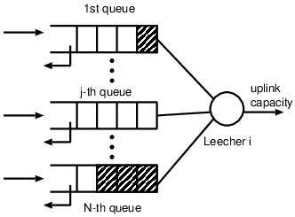
Let and be the seed and leechers’ uplink capacities, respectively. Assume that the leechers’ downlink capacities are much larger than and . Let be the number of leechers in the system at time . Since the seed always has interesting pieces to every leecher, all the queues in the seed are backlogged. Thus, all queues will be served at rate . Note that, since the swarm is unpopular, we assume the swarm size is small enough such that every leecher is neighbor of every other peer (including the seed) and can serve all of them simultaneously.
A leecher may not have interesting pieces to some of its neighbors at time . Let a leecher be identified by its arrival order, thus leecher is the -th leecher to join the swarm. Also let be the number of leechers interested in pieces owned by . The instantaneous upload rate from to any of these leechers is .
Whether a leecher has or has not pieces interesting to another depends on the leechers’ respective bitmaps, i.e. the current subsets of pieces owned by a leecher at time . The set of bitmaps of all leechers would precisely determine the exact pieces in each queue. However, the dynamics of the bitmaps are intricated and to keep track of them would be unnecessarily complicated for modeling the phenomenon we are interested in. Instead, we consider the number of pieces owned by each leecher , , and infer whether a leecher has interesting pieces to other leechers.
For the sake of simplicity, let and . Two remarks can be made with respect to and the interest relationship among leechers:
Remark 1.
If , then has at least interesting pieces to .
Remark 2.
If , it is impossible to determine whether has or has not interesting pieces to without further information.
In the following, we will use these two remarks to derive a simple model to capture the upload and download rates between peers. With respect to Remark 2, we will assume that no further information is available, and hence the piece interest relationship among peers will be ignored in this case. Nevertheless, we will see that a peer with less pieces than other can still upload pieces to the latter.
4.1 A simple fluid model
We assume that content is fluid, or equivalently, that pieces can be subdivided in infinitely many parts that can be exchanged (uploaded and downloaded) continuously.
To simplify the explanation, assume that , i.e. an older leecher has strictly more pieces than a younger one. We will relax this assumption later on this section, allowing the model to represent swarms where two peers arrived at the same time, or more generally, where some leechers have the same number of pieces. We now make the following assumptions:
- 1.
Even if leecher has joined the swarm after , i.e. , can still upload pieces to as long as downloads pieces from any peer that has more pieces than , i.e. . Thus, younger peers can upload to older peers.
- 2.
Every piece downloaded from the seed by a leecher is immediately interesting to all other leechers, independently of their arrival time. The rarest-first piece selection policy provides support for this assumption. Figure 10 depicts the idea that a younger peer can upload pieces to an older one. In this scenario, peer 4 can upload to peer 2, since it is downloading pieces interesting to peer 2 from the seed and from peer 1.

Figure 10: Peer 4 can upload pieces to peer 2, since it is downloading pieces interesting to the latter from the seed and from peer 1. - 3.
Since the seed’s upload capacity is , each leecher downloads from it at rate . Now let be the rate at which peer could potentially upload data to peer provided that there is no capacity constraints (i.e. independently of upload and download capacities of peers and , respectively). If a leecher is older than , has interesting pieces to . Therefore, from the perspective of the multiple queueing system, queue in leecher is backlogged and . On the other hand, if is younger than , the rate is given by the rate at which downloads interesting pieces to .
We draw the reader’s attention to the first two assumptions. They account for the upload rate that a younger leecher can sustain to an older leecher, even though we cannot say that the former has interesting pieces to the latter just from the number of pieces they own.
From these assumptions, we can conclude that the rate at which a peer uploads interesting pieces to an older peer is equal to the rate at which peers older than upload to plus the rate at which downloads from the seed. We thus have:
| if | (1a) | ||||
| if | (1b) |
where is the rate at which leecher uploads to .
For instance, in Figure 10, is the sum of the rates at which peer 2 downloads from the seed () and from peer 1 (). Hence, . Again we see that the proposed model accounts for the fact that a younger leecher can upload pieces to the older ones. In a real swarm however, peer 4 may upload to peer 2 pieces downloaded from younger leechers as well, such as peer 5. Although the pieces that peer 5 downloads from the seed are immediately interesting to both peers 2 and 4, they will not start and finish downloading this piece from peer 5 at the same time. Thus, leecher 4 may finish first the download of such a piece and then help serve the remaining sub-pieces to peer 2, violating our assumption. Intuitively however, the contribution of peer 4 in uploading this piece to peer 2 is small, since peer 4 must fully finish the download before it can start uploading, by which time peer 2 will have downloaded most of the piece from peer 5. Thus, we claim that such effects are negligible and can be ignored since the model is accurate when compared to simulations and experiments, as discussed in Section 4.2.
We now make an important observation concerning Equation (1b). Consider leecher and some other leecher . The older is with respect to the smaller is the rate at which can upload to , that is, the smaller is . If is younger than , then . This observation implies that .

In addition, note that for all . As we consider a small swarm, all peers upload to one another. Since the upload capacity of peers is finite, we must now determine how the capacity of a given peer will be divided to serve each of the other leechers. In particular, recall that is the upload rate from peer to peer and note that , where is the upload capacity of a leecher. To determine given the values of , where , we use a bandwidth allocation mechanism that follows a progressive filling algorithm. This mechanism determines the outcome of the processor sharing discipline. Figure 11 illustrates the progressive filling algorithm for the example presented in Figure 10. Roughly, infinitesimal amounts of bandwidth are allocated to each neighbor until (1) the leecher’s capacity is completely allocated or (2) a leecher is satisfied with respect to the constraint. In the former case, the algorithm stops. In the latter, it continues to distribute the remaining capacity among the non-satisfied leechers until one of the two conditions occurs again.
Due to the fact that , the final bandwidth allocation for leecher can be efficiently obtained by computing the following equation in the order :
| (2) |
where is the cardinality of a set . Now recall from Equation (1b) that depends on , for . Therefore, by calculating in the order , we assure that every variable in Equation (2) has been previously computed.

As an example, consider the calculation of the matrix , which determines upload rates between peers at a given moment, for a small swarm containing a single seed and leechers. Let their upload capacities be equal to kBps and kBps, respectively, and assume . Matrix and the order of computation of its elements are depicted in Figure 12. The download rate for peer is simply plus the sum of the elements in column :
| (3) |
Hence,
| (4) | |||||
| (5) | |||||
| (6) |
Equations (4)-(6) corroborate the idea that homogeneous peers can exhibit heterogeneous download rates which depend on the number of pieces owned by each leecher. Moreover, younger leechers tend to have a higher download rate, as they obtain a higher upload rate from other leechers. This is the opposite of what happens in large swarms, where the older leechers usually manage to keep the TFT for longer periods, hence achieving higher download rates.
Eventually the number of pieces owned by a leecher may reach the number of pieces owned by an older one. In particular, this is bound to occur since younger leechers tend to have a higher download rate. In this case, these two leechers will no longer have pieces interesting to each other. Thus, Equations (1b) and (2) must be rewritten as functions of :
| if | (7a) | ||||
| if | (7b) |
| (8) |
Intuitively, Equation (8) combines the two constraints on the rate at which upload pieces to . The first term stands for the maximum instantaneous rate irrespective of capacity limitations. The second term reflects the fraction of ’s uplink capacity that can be dedicated to given that some bandwidth has already been allocated. In this case, is the remaining capacity of and is the number of peers that will share it (including ). Note that the equations above relax our initial assumption that had to be distinct at all times, allowing for leechers to join the system simultaneously or more generally, for leechers to have the same number of pieces.
In Equations (7b) and (8), variables , and change over time, representing arrivals, departures and the acquiral of new pieces. Instead of writing those variables as a function of time, we dropped the variable for the sake of simplicity. Therefore, these equations can be computed for each time interval by assigning to these variables their corresponding values at that time. However, note that a change in does not necessarily imply in a change in the download rate of leechers as what matters is the relationship between and , for all . Thus, as the system evolves the variables that govern the equations will change value, but not the equations themselves, which can be used to compute the current download rate of leechers given the state of the swarm.
We will see in Section 4.2 that the proposed model given by Equations (7b) and (8) yields accurate results for unpopular swarms, indicating that for this scenario it is sufficient to know the number of pieces each peer possesses. Nevertheless, we further discuss two useful generalizations to this model in Section 4.3.
4.2 Model Validation
Our model gives an approximation to the average download rate experienced by a leecher in a unpopular swarm, which depends on the relationship between the number of pieces owned by the peers and upload capacities. In this section, we validate the model comparing its predictions with simulations results. We will see that even though the model does not take the TFT and other mechanism into account, its results are very similar to those obtained from our simulator, which implements a fully functional version of the BT protocol (see simulator description in Section 2.2).
We consider homogeneous swarms with kBps, where exactly arrivals occur. In addition, all leechers arrive before the first one completes the download and all the arrivals occur before any two leechers synchronize their contents. In our simulations, we say that two leechers and are synchronized if they have roughly the same number of pieces, i.e., . We use deterministic arrivals to reproduce the exact scenarios we intend to compare.


Consider the evolution of number of downloaded pieces in such a swarm illustrated in Figure 13a. The first leecher arrives at time and four other leechers join the swarm at . After , leechers start to synchronize. We chose several points from curves in this figure corresponding to instants of time where an event that can change peers’ download rates occurs. More precisely, we labeled points in these curves with numbers when new leechers arrive or when two leechers synchronize.
Figure 13b shows peers’ download rates from simulations and model for the labeled points indicated in 13a. We have simulated five runs for each scenario including the one depicted in this figure. The confidence intervals obtained are relatively small and are omitted.
The simulation results for points 1, 2, 4, 7, 11, 16, 20, 23 and 25 show approximately the same download rate, what is correctly captured by the model. The download rates obtained from the model are exactly the same due to fact that the corresponding peers already have every piece that was previously pushed by the seed into the swarm. Thus, neighbors of such peer can only upload to it new pieces they receive directly from the seed, i.e., their upload rate is constrained by . Since this constraint is below the capacity that can be allocated to serve a neighbor when (which is, at least ), every peer in the swarm will upload to one such peer with rate equal to . Therefore, the average download rate predicted by the model for peers in is . In particular, the relative error is less than 1.5% for all these points. The model is quite accurate even for other values of .
On the other hand, simulation results for the other points exhibit a great variety of download rates. However, those points which correspond to the same moment in time display similar download rates (e.g. 8, 9 and 10). We observe that the download rates decrease with new arrivals. We also note that as more leechers become synchronized, non-synchronized leechers achieve higher download rates (see points 21, 22 and 24). This increase in the download rates occurs because the greater is the number of synchronized peers, the greater is the remaining capacity to serve leechers with less pieces. This is due to the fact that the rate at which synchronized leechers can transmit to each other is very constrained as we discussed before. The relative error of the model is less than 1% for all points, but the 5-th (7%) and the 24-th (3%).
From these figures we conclude that when , at a given moment in time, it is possible to partition the set of leechers in two subsets: leechers with the same number of pieces as the oldest leecher (subset ), and those with less pieces than the oldest one (subset ). When , the model predicts that all leechers in each of these subsets will have identical download rates. Moreover, a leecher in will have a higher download rate than one in and this difference depends on the set sizes. In particular, larger swarms imply lower values of the minimum download rate and higher values of the maximum download for leechers in . This tendency can be observed both in simulation and model.
Considering all the simulations performed, we conclude that the model is quite accurate, with differences being unnoticeable in most scenarios and less than 10% in all cases. More importantly, the model captures well the trends observed in simulation.
4.3 Model generalizations
Some of the assumptions of the model we propose are: (1) unconstrained (or large) download capacities, and (2) leechers with identical upload capacities. We now relax the former assumption by providing an upper bound for the download rate of a peer. This bound is a function that does not grow fast on the system parameters. Clearly, if the download capacities are greater than this function then all the previously presented results hold.
In what concerns the latter assumption, we indicate how to adapt the model to cope with similar (but not identical) upload capacities. Furthermore, we present some simulation results that show that the general behavior of the system under this scenario is similar to the one presented in Section 3.
4.3.1 Finite (and small) download capacities
When the oldest peers are synchronized, they can only send to each other what they receive directly from the seed (see Equation (7b)). This constraint leads to more capacity available to serve those peers that are not synchronized. In particular, if there is only one non-synchronized peer, it can benefit from this idle bandwidth alone and consequently achieve the highest possible download rate. In what follows we compute an upper bound for this maximum download rate.
Consider an unpopular swarm with peers, such that the oldest peers are synchronized. From Equation (7b) we can compute the maximum instantaneous upload rate of a synchronized leecher to the other peers irrespective of capacity limitations:
| if j is not synchronized | (9a) | ||||
| if j is synchronized | (9b) |
According to Equation (8), each leecher will upload to each of the other synchronized peers at rate . The remaining capacity of that can be used to serve the younger leecher is . Since there are synchronized leechers, the capacity that can be used to serve only non-synchronized leecher is . In addition, the younger leecher downloads from the seed at rate . Therefore, the maximum download rate is given by
Thus, we have:
| if | (10a) | ||||
| otherwise | (10b) |
Note that in both cases the maximum download rate is a value that does not grow fast in any of the system parameters. In particular, for small , which is the case of interest, has a relative small value with respect to the upload capacities or leechers and seed. Thus, if the download capacities of leechers are larger than , then results predicted by the model are just as good. This condition replaces the requirement of unbounded (or arbitrarily large) download capacities assumed earlier in the model.
To illustrate, consider the example in Section 4.2 where kBps and . In this case, the highest download rate would be kBps. Thus, if download capacities of leechers are larger than 140.8Kbps, then the results predicted by the model would be unchanged.
4.3.2 Similar but not identical upload capacities
Although we have assumed upload capacities of peers to be identical, this is certainly not necessary for the piece distribution process in unpopular swarms to lead to heterogeneous download rates. Note that our modeling framework allows for peers to have different upload capacities, as could depend on in Equation 2 (equivalently, in Equation 8). Clearly, this would have an impact on the heterogeneity of the performance and would depend on the values of and the order of their arrivals to the swarm. However, if are close to one another, for example, chosen uniformly at random from a small range, then we expect not to see much differences with respect to the constant value.
In order to support this last claim, we repeat the simulations described in Section 3.2 but allowing the upload capacity of leecher to be drawn uniformly at random from the range , where kBps and . Figures 14(a-b) show the average download time of peers binned according to the number of leechers in the swarm at the arrival time for and , respectively. We conclude that, when the upload capacities are close to each other, the system exhibits a very similar behavior to that we observed when the upload capacities are the same (see Figure 4). Not surprisingly, the larger the range of upload capacities, the the greater the impact on the results, when compared to a constant upload capacity.


.
5 Predicting bursty departures
The model presented in Section 4 can be used to estimate the number of departures that occur in a burst. In particular, consider the arrival of a leecher that initiates a busy period (i.e., the first arrival to a swarm with no leechers). In the following, we estimate the average number of peers that depart the swarm in a burst together with the leecher that initiated the busy period.
In practice, bursty departures do not occur exactly at the same time due to variations inherent to the network and to the inexistence of mechanisms that enforce synchronization between peers implemented in the protocol (e.g.: they do not request pieces at exactly the same time). Nonetheless, our model does not take these factors into account and, thus, we focus on leechers that leave the swarm at exactly the same time as the first leecher.
Let denote the first leecher of a busy period and assume that the leecher arrival follows a Poisson distribution with rate . Also, as assumed by the model, a seed is always present and has uplink capacity of , while leechers have identical uplink capacities equal to . Finally, let denote the number of pieces of the content.
We know that each leecher downloads pieces from the seed at rate , where is the number of peers in the swarm. These pieces are interesting to all the other peers and can be sent to them. Thus, if , leechers will start to accumulate pieces received from the seed which cannot be uploaded to the other peers. Therefore, every leecher will own pieces interesting to all of its neighbors. Consequently, the upload rate between any two leechers and will be equal to , since (see Equation (8)). We conclude that when , all leechers have the same download rate which prevents other leechers from departing in a burst with .
Conversely, when , the neighbors of can upload to it the pieces they download from the seed. Since leecher downloads from the seed at rate and each of its neighbors receives pieces from the seed and uploads them to at the same rate, will download the content at a constant rate equal to , independently on the number of peers in the swarm. Note that is also the upper bound on the average download rate, as the seed cannot uploads pieces into the swarm at a faster rate. Hence, leecher will take seconds to finish the download.
We now show how to calculate the lower and upper bounds to the number of bursty departures when . Consider arrivals that occur while peer is in the swarm. The number of such arrivals, say , is a random variable and follows the Poisson distribution with parameters and . The download rates of these leechers are a function of and also of their instants of arrival. Moreover, as discussed in Section 4.2, larger values of imply a larger spread in the download rates. To obtain a conservative lower and upper bound on these download rates, we will consider a sufficiently large value for . In particular, we use the 99-th percentile of , namely , and thus, .
Given that exactly leechers will join the swarm before the departure of , we can use the model to obtain the minimum and maximum download rates of these peers, independently of their inter-arrival timing. Let and be, respectively, the minimum and the maximum download rates obtained from the model given that the swarm has leechers.
Consider again the subsets presented in the previous section, namely (leechers with the same number of pieces than ) and (leechers with less pieces than ). The minimum download rate is obtained by a leecher in when the only leecher in is . In this case, the download rate is given by
| (11) |
where corresponds to the sum of the rates at which downloads from peers in .
On the other hand, a leecher in obtains the maximum download rate when it is the only peer in , i.e, . In this case, the download rate is given by
| (12) |
The minimum and maximum time for the leechers to download the content is, respectively, and . Therefore, at least all leechers that arrive before will leave the swarm together in a burst with . The expected number of peers that will arrive within this time period, is simply given by
| (13) |
Similarly, at most all leechers that arrive before will leave the swarm in a burst with . The expected number of peers that will arrive within this time period, is simply given by
| (14) |
Finally, and provide a lower and upper bound for the average number of leechers that will depart the swarm in a burst with .
| (kBps) | |||||
|---|---|---|---|---|---|
| 48 | 5.333 | 1.667 | 4.378 | 0.312 | 0.821 |
| 64 | 4.000 | 0.400 | 1.895 | 0.100 | 0.474 |
Table 2 shows the expected number of arrivals to the swarm before departs, , which is simply , and both the lower and upper bounds and , respectively. The table shows numerical results for different values but with kBps and . The results indicate that average number of peers that depart the swarm in a burst with can be significant: between 31% and 82% of all arrivals when the seed is slower than the leechers and between 10% and 47% when they have the same upload capacity. We also observe that these ratios reduce as increases, indicating that bursty departures are less likely to occur with faster seeds. Recall that, as indicated above, there is a minimum value of for which bursty departures do not occur.
6 General discussions
We now discuss other aspects related to the described phenomenon such as different arrival processes, what happens if the seed is not available all the time, what happens when leechers stay as seeds for some time and the missing piece syndrome.
6.1 General arrival processes
It is interesting to consider the occurrence of the observed phenomenon in more general scenarios. Although we have shown its prevalence under a crafted peer arrival process and under Poisson arrivals, we claim that homogeneous peers can have heterogeneous download rates under very general arrival patterns. In particular, given any arrival pattern of peers into a swarm, it is possible to choose system parameters (i.e., seed upload capacity, leechers upload capacity, and file size) such that the effects described in this paper will be very prevalent. Intuitively, by choosing a fast enough seed, peers will not be able to disseminate old pieces before new ones are pushed into the swarm, and thus will have significantly different number of blocks. In a sense, the behavior observed and described in this paper is quite general, although the requirement of the swarm being unpopular is important, as we next describe.


What happens if we consider very popular swarms, where the peer arrival rate is very large, yielding very large swarm sizes? Figure 15a shows experimental results of the dynamics of leecher arrivals and departures for this scenario (Poisson arrivals with rate , uplink capacities of kBps and kBps) and file size pieces (i.e., 20 MB). The empirical CCDF of the download time is depicted in Figure 15b. Interestingly, we can still observe the consequences of having heterogeneous download rates, such as bursty departures, content synchronization and high variability of download times (peers that leave in a large burst have different download times, as arrival is well-behaved), for example, at times 600 s and 1200 s. In a sense, the phenomenon is quite prevalent even during the busy period, but not strong enough to end the busy period. The characterization and modeling of the phenomenon in this scenario is much more entailed, given the complicated dynamics of piece exchange of BT and consequently the interest relationship among peers. We leave the investigation of these scenarios (popular swarms) as future work.
6.2 When the seed is not available all the time
We have considered so far swarms that have a single seed which is always connected. However, what happens if the seed alternately joins and leaves the swarm? Intuitively, leechers start to synchronize their contents right after the seed leaves because no new pieces are being placed into the swarm. After they become fully synchronized, they will stall until the seed comes back. Then, since they are synchronized, they will have relatively low download rates and will leave almost at the same time. Therefore, the intermitent seed makes the average download rates even more heterogeneous.
In order to support this claim, we modify the simulation model such that the state of the seed (connected/disconnected) is given by an ON-OFF source. We assume that the time until the seed leaves the ON state (leaves the swarm) is exponentially distributed with rate (arbitrarily set to be equal to the leecher arrival rate). Furthermore, we choose the rate at which the seed goes from the OFF back to the ON state (rejoins the swarm) so that the availability of the seed is , and .
Table 3 summarizes the results for s, kBps, pieces. Each scenario was simulated during s. We observe that the mean, variance and maximum download time monotonically increase, what is expected as there are less resources on average. Interestingly, the minimum download time becomes smaller. This is due to the fact that a a new leecher may arrive when some peers are stalling in the absence of the seed, just before finishing the download. The new leecher then benefits from the spare bandwidth capacity and might complete the download right after the seed comes back. Finally, it is clear the download time (equivalently, download rate) becomes more heterogeneous.
| Mean | Variance | Minimum | Maximum | |
|---|---|---|---|---|
| 1.00 | ||||
| 0.75 | ||||
| 0.50 | ||||
| 0.25 |
Note that, in fact, the proposed analytical model can cope with this scenario as long as peers do not accumulate pieces interesting to each other, i.e. (see Section 5). In particular, if the seed departs, then this will only affect the upload rate among peers, given by Equation (1b) (or Equation (7b)). More precisely, the term corresponding to the download rate from the seed () should be set to zero in the equations that describe time periods where the seed is not present. Thus, given the state of the swarm with respect to the seed’s presence and number of leechers, we can still apply our modeling framework and determine the download rates of leechers (under the condition above).
6.3 When leechers stay as seeds for some time
Another aspect that can be taken into account is that leechers may stay as seeds for a period of time after they finish the download and before leaving the swarm. Intuitively, since the capacity available to disseminate the file increases as leechers stay as seeds, peers concurrently downloading a file tend to receive pieces at similar download rates, possibly reducing the consequences of heterogeneous download rates. We performed simulations for scenarios where s, kBps, pieces and the time which leechers stay seeding is deterministic and equal to . Each scenario was simulated 10 times during 400,000 s, but the first 100,000 s were discarded to avoid transient effects. Figures 16(a)-(c) depict the results for many values of .
As indicated in Figure 16a, bursty departures are less likely to occur when leechers stay in the swarm after downloading the entire content. However, for small values of (with respect to ), the difference is barely noticeable and the departure process is still very bursty.
Figure 16b shows the CCDF of leechers’ download times for different values of while Table 4 contains statistics of these distributions, namely the sample mean and variance, minimum and maximum values. Intuitively, leechers that find two or more seeds at arrival time have significant better performance and hence the minimum download time decreases as the seeding time increase. On the other hand, the maximum download time is the approximately same for the majority of the curves. This is because there is a non-zero probability that a leecher downloads the content entirely from a single seed. However, this probability becomes smaller with the seeding time. Initially the variance increases with , but when leechers stay as seeds for a long period of time, it is unlikely that a leecher will have a download time much larger than the average and thus, the sample variance diminishes (see 5,000 and 10,000 in Table 4).
Finally, Figure 16c shows that while early arrivals are detrimented for small values of , they are benefited when is high. The presence of multiple seeds has the same effect as a single seed with higher capacity. This can be observed by comparing the curves for equal to 5,000 and 10,000 and the curve corresponding to kBps in Figure 4.


| Mean | Variance | Minimum | Maximum | |
|---|---|---|---|---|
| 0 | ||||
| 100 | ||||
| 500 | ||||
| 1000 | ||||
| 2000 | ||||
| 5000 | ||||
| 10000 |
6.4 Missing piece syndrome
Last, we now comment on the relationship of our findings and the phenomenon known as missing piece syndrome. This phenomenon states that in swarms where the arrival rate is large enough, the system can become unstable (i.e., number of leechers grows unboundedly) if the upload capacity of the seed is not large enough [9, 10, 11]. The key aspect of this syndrome is content synchronization, where a large fraction of peers have all but one and the same piece. This situation is particularly bad to the performance of the swarm, as the departure rate of the swarm will be equal to the seed upload capacity (assuming peers depart as soon as they acquire the last block). Our work has shown that peers can synchronize their content in such a way that several identical pieces are missing which eventually leads to the missing piece syndrome. In some sense, this generalizes the syndrome to a piece synchronization syndrome, which is inherent to BT dynamics due to the heterogeneous download rates as discussed in this work. Once peers have synchronized their content, they can only acquire new pieces from the seed, at the upload capacity of the seed. In this scenario, the missing piece syndrome is bound to occur.
7 Related prior works
Modeling P2P file sharing systems and in particular BT has been an active area of research in the past few years, driven mainly by the high complexity, robustness and user-level performance of such systems. One of the first BT models to predict the download times of peers was presented in [6]. This simple fluid model based on differential equations assumes homogeneous peer population (with respect to download and upload capacities) and Poisson arrivals, but yields analytical steady state solution for performance metrics. Several subsequent BT models have been proposed in the literature to capture various system characteristics, among them heterogeneous peer population (with respect to upload and download capacities) [18, 7, 19, 8]. However, to the best of our knowledge, all models predict that identical peers (with respect to their upload capacities) simultaneously downloading a file will have similar performance (with respect to download rates), contrary to the findings in this paper. Moreover, BT models generally assume either a rather large peer arrival rate (e.g., Poisson) or a large flash crowd (all peers join the swarm at the same time). This is somewhat surprising, given that most real BT swarms are rather small in size and quite unpopular [12]. Finally, one perverse effect of this lack of popularity, known as content unavailability, is shown to be a severe problem found in most of BT swarms [20].
Another interesting aspect of BT has been the discovery and characterization of some non-trivial phenomena induced by its complex dynamics. For example, peers in BT swarm tend to form clusters based on their upload link capacities, exhibiting a strong homophily effect. In particular, peers with identical upload capacities tend to exchange relatively more data between them [21, 22, 23]. Yet another peculiar behavior is the fact that arriving leechers can continue to download the entire content despite the presence of any seed in the swarm, a property known as self-sustainability [24]. More recently, the missing piece syndrome has been characterized mathematically [10, 11]. In [25] is presented an evaluation for the impact of different peer selection strategies on the stability of the system. Such strategies may reduce the effect of content synchronization among peers. However, to the best of our knowledge, we are not aware of any prior work that has alluded the phenomenon we describe in this paper, namely, that homogeneous peers can have heterogeneous download rates.
8 Conclusion
This paper identifies, characterizes and models an interesting phenomenon in BT: homogeneous peers (with respect to their upload capacity) experience heterogeneous download rates. The behavior is pronounced in unpopular swarms (few leechers) and has important consequences that directly impact peer and system performance. The mathematical model proposed captures well these heterogeneous download rates of peers and provides fundamental insights into the root cause of the phenomenon. Namely, the allocation of system capacity (aggregate uplink capacity of all peers) among leechers depends on the piece interest relationship among peers, which for unpopular swarms is directly related to arrival order of peers and can be significantly different among them.
Acknowledgment
This research was supported in part by grants from CAPES, CNPq FAPERJ (Brazil) and NSF under the grant CNS-1065133.
References
- [1] F. Murai, A. A. de A. Rocha, D. R. Figueiredo, E. A. de Souza e Silva, Heterogeneous download times in a homogeneous BitTorrent swarm, Computer Networks 56 (7) (2012) 1983–2000. doi:https://doi.org/10.1016/j.comnet.2012.02.009.
- [2] B. Cohen, Incentives build robustness in BitTorrent, in: P2PECON, 2003.
- [3] Ipoque internet study, http://www.ipoque.com/news_&_events/internet_studies/internet_study_2007 (2007).
- [4] R. L. Xia, J. Muppala, A survey of bittorrent performance, IEEE Communications Surveys & Tutorials (2010). doi:10.1109/SURV.2010.021110.00036.
- [5] X. Yang, G. de Veciana, Service capacity of peer to peer networks, in: IEEE INFOCOM, Vol. 4, 2004, pp. 2242 – 2252.
- [6] D. Qiu, R. Srikant, Modeling and performance analysis of bittorrent-like peer-to-peer networks, in: ACM SIGCOMM, 2004, pp. 367–378. doi:http://doi.acm.org/10.1145/1015467.1015508.
- [7] W.-C. Liao, F. Papadopoulos, K. Psounis, Performance analysis of bittorrent-like systems with heterogeneous users, Performance Evaluation 64 (9-12) (2007) 876 – 891, IFIP Performance 2007. doi:DOI:10.1016/j.peva.2007.06.008.
- [8] A. Chow, L. Golubchik, V. Misra, Bittorrent: An extensible heterogeneous model, in: IEEE INFOCOM, 2009, pp. 585 –593. doi:10.1109/INFCOM.2009.5061965.
- [9] F. Mathieu, J. Reynier, Missing piece issue and upload strategies in flashcrowds and p2p-assisted filesharing, AICT/ICIW 0 (2006) 112.
- [10] B. Hajek, J. Zhu, The missing piece syndrome in peer-to-peer communication, in: IEEE ISIT, 2010, pp. 1748 –1752. doi:10.1109/ISIT.2010.5513266.
- [11] J. Zhu, B. Hajek, Stability of peer to peer systems, in: ACM PODC, 2011.
- [12] L. Guo, S. Chen, Z. Xiao, E. Tan, X. Ding, X. Zhang, A performance study of Bittorrent-like peer-to-peer systems, IEEE JSAC 25(1) (2007) 155–169.
- [13] S. Kaune, R. C. Rumín, G. Tyson, A. Mauthe, C. Guerrero, R. Steinmetz, Unraveling bittorrent’s file unavailability: Measurements and analysis, in: IEEE Tenth International Conference on Peer-to-Peer Computing (P2P 2010), 2010, pp. 1–9.
- [14] T. Hossfeld, F. Lehrieder, D. Hock, S. Oechsner, Z. Despotovic, W. Kellerer, M. Michel, Characterization of bittorrent swarms and their distribution in the internet, Computer Networks 55 (5) (2011) 1197–1215.
- [15] A. Legout, G. Urvoy-Keller, P. Michiardi, Rarest first and choke algorithms are enough, in: ACM IMC, 2006, pp. 203–216. doi:http://doi.acm.org/10.1145/1177080.1177106.
- [16] E. de Souza e Silva, D. R. Figueiredo, R. M. Leão, The TANGRAM-II integrated modeling environment for computer systems and networks, SIGMETRICS Perform. Eval. Rev. 36 (2009) 64–69.
- [17] L. Peterson, A. Bavier, M. E. Fiuczynski, S. M. Ly, Experiences building planetlab, in: USENIX OSDI, 2006, pp. 351–366.
- [18] F. Lo Piccolo, G. Neglia, The effect of heterogeneous link capacities in bittorrent-like file sharing systems, in: Hot-P2P, 2004, pp. 40 – 47. doi:10.1109/PTPSYS.2004.21.
- [19] M. Meulpolder, D. Epema, H. Sips, Replication in bandwidth-symmetric bittorrent networks, in: IEEE IPDPS 2008, 2008, pp. 1 –8. doi:10.1109/IPDPS.2008.4536194.
- [20] D. Menasche, A. Rocha, B. Li, D. Towsley, A. Venkataramani, Content availability and bundling in swarming systems, in: ACM CoNEXT, 2009, pp. 121–132.
- [21] A. Legout, N. Liogkas, E. Kohler, L. Zhang, Clustering and sharing incentives in bittorrent systems, ACM SIGMETRICS Perform. Eval. Rev. 35 (1) (2007) 301–312. doi:http://doi.acm.org/10.1145/1269899.1254919.
- [22] A. R. Bharambe, C. Herley, V. N. Padmanabhan, Analyzing and improving a bittorrent networks performance mechanisms, in: IEEE INFOCOM, 2006, pp. 1 –12. doi:10.1109/INFOCOM.2006.328.
- [23] F. Murai, A. Rocha, D. R. Figueiredo, E. de Souza e Silva, Can identical BitTorrent peers experience different download times?, in: IFIP WG 7.3 Performance 2010 Poster Abstracts, Namur, Belgium, 2010, pp. 29–30, extended Abstract.
- [24] D. S. Menasché and A.A. Rocha and E. de Souza e Silva and R.M. Leão and D. Towsley and A. Venkataramani, Estimating self-sustainability in peer-to-peer swarming systems, Performance Evaluation 67 (2010) 1243–1258. doi:DOI:10.1016/j.peva.2010.08.013.
- [25] D. Menasche, A. Rocha, E. de Souza e Silva, D. Towsley, R. Leao, Implications of peer selection strategies by publishers on the performance of p2p swarming systems, Performance Evaluation Review (2011).