Remarks on the effects of quantum corrections on moduli stabilization and de Sitter vacua in type IIB string theory
Vasileios Basiouris 11 1 E-mail: v.basiouris@uoi.gr, George K. Leontaris 22 2 E-mail: leonta@uoi.gr
Physics Department, University of Ioannina
45110, Ioannina, Greece
The rôle of string loop corrections on the existence of de Sitter vacua and the moduli stabilization problem is examined in type IIB effective theories. The fundamental building blocks are a minimum of three intersecting D7 brane stacks, three Kähler moduli, and a novel Einstein-Hilbert term associated with higher derivative terms of the 10-dimensional effective action. It was shown in previous works that loop corrections appear which induce novel logarithmic volume-dependent terms in the effective potential. When D-term contributions are considered, all Kähler moduli are stabilized and de Sitter vacua are achieved. In the present work, a comprehensive study of multiple non-perturbative terms in the superpotential is undertaken. The combined effects of the logarithmic loop corrections and two non-perturbative superpotential Kähler moduli dependent terms have been investigated. It is shown that a variety of fluxes exist for large as well as moderate volume compactifications which define a de Sitter space and stabilize the moduli fields. For large volumes, a generic simple form of the potential is achieved. The so obtained effective potential appears to be promising for cosmological applications.
1 Introduction
There has been a lot of recent activity regarding the implications of quantum corrections to the moduli stabilization problem and the existence of de Sitter (dS) vacua in effective string theory models. These investigations are significant for providing an answer of whether the otherwise presumably consistent effective theories have an ultraviolet completion, and as such, they could be accommodated in the string landscape33 3 There is a vast literature on this issue. For the recent debate on Swampland conjectures see for example [1, 2, 3] and related reviews [5, 6, 4]. Also, an incomplete list of 10d supergravity dS solutions and other related issues is [8, 9, 10, 11, 7, 12, 13]. These explorations are also of great importance since they are related to the accelerated expansion of the universe and the scenario of cosmological inflation.
An appropriate framework to investigate the effects of quantum corrections is type IIB string theory and, more generally, F-theory defined on an elliptically fibered Calabi-Yau (CY) fourfold. The fundamental constituents of the effective field theory (EFT) emerging after compactification of the ten-dimensional theory to four dimensions on a CY manifold, are the superpotential and the Kähler potential which is of no-scale type. The basic ingredients are the various types of moduli fields associated with the various deformations of the compactification, D-brane stacks with magnetic fluxes and topological parameters such as the Euler characteristic. At the classical level of the resulting EFT a number of pertinent issues arise. The tree-level superpotential is a function of the various types of those fields, including the axion-dilaton and the complex structure moduli, however, it does not depend on the Kähler ones. Supersymmetric conditions imposed on in principle can fix the values of all but the Kähler moduli. On the other hand, the scalar potential vanishes identically due to the no scale structure of the Kähler potential and as a consequence, the Kähler moduli remain undetermined. Moreover, a vanishing scalar potential cannot describe the accelerated expansion of the universe which requires a positive cosmological constant, that is, a dS minimum.
The way to confront these issues is to incorporate quantum corrections in and functions. The superpotential receives non-perturbative corrections appearing through exponential terms which depend on the Kähler (volume) moduli (see for example [14] and [15])44 4 For recent developments on related work see [16, 17, 18, 19, 20, 21, 22, 23]. In the context of type IIB string theory the Kähler potential receives perturbative corrections where the leading order is [24]. Recently, the effects of gravitational terms beyond the standard Einstein-Hilbert term have been considered in the context of a geometric configuration involving three brane stacks intersecting each other. The terms next to leading order in the low-energy expansion of type II superstring are fourth order () in the Riemann curvature , which do not receive any perturbative corrections beyond one loop [25, 26, 27, 28, 29]. Dimensional reduction of the ten-dimensional string effective action in four dimensions induces an additional Einstein-Hilbert term appearing in the bulk multiplied by a factor proportional to the Euler characteristic. The amplitude induced by graviton scattering involving two massless gravitons and a Kaluza-Klein (KK) excitation propagating towards a brane stack yields logarithmic contributions breaking the no scale invariance of the Kähler potential [30, 31]. This induces an F-term anti de Sitter scalar potential whereas symmetries associated with the brane stacks provide the necessary uplift to a dS minimum through positive D-term contributions to the scalar potential. Both, logarithmic corrections and D-terms are sufficient to stabilize the Kähler moduli and support a positive cosmological constant. Also, the implications of this construction on the cosmological inflation have been studied. It was found that hybrid inflation is successfully implemented with the internal volume modulus acting as the inflaton [32], and the rôle of the waterfall field is played by open string excitations associated with the brane stacks [33].
Within the above context, in a previous work [34] a first step towards combining the effects of the logarithmic (perturbative) and the non-perturbative corrections has been put forward. The analysis was performed within a framework of three Kähler moduli and three intersecting brane stacks and, on first approach, only one Kähler modulus has been considered to contribute in the flux induced superpotential through an exponential term of the form . A circumstantial study of the scalar potential revealed regions of the fluxes and other parameters 55 5 While several properties of the effective model emerging from String theory are already fixed, yet, there are free parameters such as the Euler characteristic related to the compactification manifold and the various magnetic fluxes on branes which define the final shape of Quantum Corrections. supporting dS minima in agreement with the present day cosmological observations.
Usually, however, in realistic compactification scenarios more complicated situations arise where several Kähler moduli induce non-perturbative terms in the superpotential. In the present work, a useful extension of the previous analysis with two such terms (involving two distinct Kähler moduli) is performed, which captures many features of previous models. For example, an analogous situation with two exponential terms arises where such type of exponential terms in the superpotential are introduced when E3-instantons wrap two cycles[35]. Also, in the limiting case where the two exponentials depend on the same Kähler modulus, the present construction reduces to the particular racetrack paradigm studied in the past [36].
Taking into account the above remarks, the objective of the subsequent analysis is the investigation of the combined effects of perturbative and non-perturbative contributions to the scalar potential of the effective theory. Regarding the perturbative loop corrections, of particular interest in this work are those related to novel graviton kinetic terms in the bulk which receive logarithmic corrections due to the emission of closed strings propagating in a two dimensional space towards probes. In the Kähler potential (denoted with ), these corrections appear as a shift to the internal volume , breaking its no scale structure whereas this logarithmic dependence of the Kähler (volume) moduli is conveyed to the scalar potential of the effective theory through . Hence, these corrections imply a structure of the potential -analogous to that realizing the Coleman-Weinberg mechanism [37]- which depends on the Kähler moduli and only a few parameters such as the magnetic fluxes and topological invariants of the compactification manifold.
In the following section, (section 2), the basic features of the model together with a short review of the previous work [30, 31, 34] are presented. In section 3, the scalar potential is computed taking into account the aforementioned perturbative logarithmic contributions and the non-perturbative corrections. In section 4, D-term contributions are included. A simple form of the total potential is presented in the large volume regime which shows that all moduli directions are stabilized along a metastable dS minimum. Section 5 deals with the search of dS solutions for moderate values of the Kähler moduli. A summary of the work and conclusions are described in section 7 and some computational details are found in the Appendix.
2 A short review and extension of previous work
In [34] a model consisting of a geometric configuration of three branes and three Kähler moduli based on the construction proposed in [30] in the framework of type IIB string theory, has been studied beyond the tree-level approximation, by including logarithmic perturbative [31] as well as non-perturbative corrections. Despite the complicated structure of these contributions, it was shown that, in the large volume regime, the scalar potential of the emerging effective field theory receives a simplified form which illustrates all the essential features of the model. Within this context, the properties of the effective potential regarding the Kähler moduli stabilization and the search for de Sitter vacua have been studied and the main findings are recapitulated here. Starting with notations and conventions, the Kähler moduli are denoted with
| (1) |
where are related to the RR -form potential and are four-cycle volumes. In terms of the latter, in the present work, the internal volume is written as follows
| (2) |
The flux induced superpotential at the classical level depends on the complex structure moduli , and is given by the Gukov-Vafa-Witten formula [38]
| (3) |
The symbol represents the combination of the field strengths and the axion-dilaton modulus . Also, are zero- and two-form potentials, is the Kalb-Ramond field, and the holomorphic three-form which depends on the complex structure moduli denoted hereafter with . Supersymmetric conditions imposed on stabilize the dilaton and -in principle- the complex structure moduli (for recent activity on this issue see section 3). However, the Kähler structure ones, , do not appear in the tree level superpotential and thus their values remain undetermined. Moreover, as it is described in well known non-renormalization theorems for fluxed superpotentials in string theory [39], cannot receive perturbative corrections to any order and the only possible contributions are of non-perturbative type. Regarding the Kähler moduli fields, non-perturbative corrections may arise from several sources including branes wrapping four-cycles and gaugino condensation on -brane stacks. In general all three moduli of the present construction may contribute, hence the generic form of superpotential is
| (4) |
In (4) the flux induced part will be considered constant evaluated by the formula given in (3). The coefficients are functions of , and are small parameters which in the case of gaugino condensation take the form , with the rank of the corresponding gauge group of the brane stack. In [34] the simplest scenario of only one Kähler modulus field (say ) was considered to have non-vanishing non-perturbative (NP) contributions so that the superpotential (4) reduces to .
The second important ingredient is the Kähler potential which depends logarithmically on the Kähler fields , the complex structure moduli through the 3-form , and the axion-dilaton field . At tree level this reads
| (5) | |||||
where in the second line the formulae (1) and (2) have been implemented.
It has been shown [31] that the argument of the logarithmic term of the Kähler potential (5) receives perturbative logarithmic corrections of the form , where is a negative constant () and depends on the Euler characteristic of the compactification manifold. As a result, the induced effective scalar potential includes logarithmic terms which are expressed in terms of the internal volume modulus . In addition, the total F-term potential involves other terms with different (power-law) dependence on . In effect, the structure of the potential is reminiscent of the Coleman-Weinberg mechanism [37] and its minimum is found at finite values of the volume modulus.
Furthermore, additional D-terms of the form associated with the universal factors of the brane stacks
can be included.
When all these components are taken into account, in the large volume limit
the scalar potential can be approximated as follows (see Appendix for details)
| (6) |
The parameter has been considered in the large volume limit to be , and is defined as the product . Hence, the two (unspecified yet) constants and in (6) multiply the F- and D-term parts respectively. Comparing the effective potential (6) with that obtained in [30] -where only perturbative corrections are taken into account- it is observed that the latter contains an additional term . This term, however, can be absorbed in the D-part of under a redefinition of the constant . As it has been demonstrated in [34], for given and , as long as the ratio of the D- and F-term coefficients is bounded in the narrow region, a dS minimum is attainable and all three Kähler moduli are stabilized.
2.1 The superpotential with two non-perturbative terms
As it has been emphasized above, the case of a single non-perturbative term in the superpotential ensures moduli stabilization and the existence of a dS vacuum as long as perturbative logarithmic corrections and D-term contributions are included. However, due to the variety of compactification manifolds the case of non-perturbative contributions from more than one moduli is a more likely scenario. Given the fact that the shape of the potential near the minimum is of particular importance for cosmological applications, (and in particular, inflation) it is worth exploring more involved situations. The purpose of the present work is to extend the previous analysis, within the same geometric configuration of three branes, and examine the implications when the flux induced superpotential , receives non-perturbative corrections from two Kähler moduli, and . In this case the superpotential takes the form
| (7) |
Cases with two exponentials capture many new features and have been discussed in the literature in particular constructions. Generically, one would anticipate non-perturbative corrections in every direction of the moduli space. It is possible, however, that world volume fluxes can in principle modify the effective action through lifting certain fermionic zero-modes, which could prohibit a particular contribution in the superpotential [40]. In the present analysis this mechanism is considered to eliminate from the exponential term involving the modulus . In a recent work for example, the two exponential terms are generated by E3 instantons wrapping appropriate singularities [35]. Also, the racetrack form [36] suitable for cosmological applications could be considered as a particular case when both exponents of (7) involve the same modulus, i.e., when in replaced with in the second exponential. In general, two or more exponential terms imply a richer structure for the shape of which could exhibit saddle points between different vacua of the theory, so that successful types of inflationary scenarios can be realized [41]. Despite the vast literature devoted on such issues, the combined effects of (7) with perturbative logarithmic corrections to the Kähler potential have not been investigated so far. These ingredients are a generic feature of the effective theories derived from the 10-dimensional superstring action and thence it is the main subject of the subsequent analysis.
Starting with the superpotential of the effective theory, while recalling that in general the coefficients and depend on the complex structure moduli , it can be readily inferred that supersymmetric conditions imposed on (7) can fix the axion-dilaton field and . Since receive masses of order whilst Kähler masses arise through the non-perturbative corrections, the former are expected to be much larger and can be integrated out [42]. Thence the last two logarithmic factors of (5) involving these fields can be treated as constants.
2.2 The Kähler potential
When various types of perturbative corrections are included, the no scale structure of the classical Kähler potential (5) is no longer preserved. Of crucial importance in the present study, are the higher derivative terms of the 10-d string action, which are responsible for multigraviton scattering. Indeed, it was found in [31] that in combination with intersecting D7-branes and planes included in the present geometric configuration, volume dependent logarithmic corrections are induced in the Kähler potential. For the sake of completeness the basic steps of their derivation are resumed in the following.
In the 10-d action the terms next to leading order in curvature are proportional to [26],[27],[29]:
| (8) |
where and are the -dimensional Ricci scalar, manifold and dilaton respectively. Compactifying six dimensions on a CY manifold , so that with the Minkowski space, while taking into account the tree-level and one-loop generated EH terms, the ten-dimensional action reduces to
| (9) |
where is the Euler characteristic defined as
| (10) |
This way a localized EH term is generated, with a coefficient proportional to the Euler characteristic , whose existence is possible only in four dimensions. In the case of type IIB string theory compactified on the which will be considered in this work, non-zero values are concentrated at the fixed points of the orbifold group. Moreover, localized vertices associated with the induced EH term, emit gravitons and Kaluza-Klein (KK) excitations in the 6-dimensional space. A useful notion related to this mechanism is the localization width which can be estimated by computing the graviton scattering involving two massless gravitons and one KK excitation. It is found that [43]
| (11) |
with the fundamental string length and the integer (which is arbitrary in the non-compact limit) is associated with the Euler characteristic .
Due to branes and orientifold planes of the assumed geometric configuration, there can be an exchange of KK-modes between the localized gravity position identified with some orbifold fixed-point, and the distinct D7-branes. Because the latter occupy four internal dimensions, KK-modes transmitted towards each one of them propagate in a two-dimensional bulk transverse to . This way, logarithmic contributions are induced depending on the size of the two-dimensional space transverse to . Thus, in addition to the one loop contribution, there are also logarithmic corrections. Referring to the relevant works for the details [43], one finds that the corresponding term of the effective action becomes:
| (12) |
where is the tension of the brane and the size of the 2-d space transverse to the corresponding . From (12) it can be deduced that the quantum corrections are of the form
| (13) |
The constant is proportional to the Euler characteristic and in the case of orbifolds for example, is given by .
Incorporating these quantum corrections in the Kähler potential while substituting from (1) the corrected Kähler potential (5) becomes
| (14) |
where stand for terms involving complex structure moduli and the axion-dilaton, as in (5). Assuming for simplicity that all branes have the same tension proportional to , the coefficients take a common value , and Eq.(14) yields
| (15) |
2.3 The supersymmetric conditions
In the present setup, the contribution of the moduli in the superpotential enters through the non-perturbative corrections, and thus, the appropriate flatness conditions must be imposed. The latter imply the vanishing of the corresponding covariant derivatives . Introducing the expansions with respect to and in the large volume limit, it is readily found that
| (16) | ||||
| (17) |
where stand for the following ratios :
| (18) |
If some reasonable assumptions concerning the various flux parameters and the range of moduli fields are made, the solutions of the above transcendental equations can be expressed in closed form with good accuracy, in terms of known functions. A possible choice of the approximations can be better perceptible as follows: The two equations (16) and (17) are combined to give
| (19) |
Since are positive constants, it turns out that , while real solutions of (16,17) exist as long as . The equation (19) is plotted in figure (1) for several values of in the parametric space defined by the pair (). The curves of the left panel correspond to values and the ones on the right, to . (For a trivial solution exists represented by the diagonal, not shown in the figure). The parametric space has been split into four regions with respect to the ranges of and . Region corresponds to large values of and thus, both terms of the non-perturbative contributions in (7) are suppressed. In general, in the large volume regime, perturbative logarithmic corrections are expected to prevail.
In the opposite limit, region corresponds to small values of , and both NP-contributions become sizable, however, in this case large requires -values much bigger than . A drawback of this region is that non-perturbative corrections correspond to the large coupling regime and as such they are not fully controllable. Nevertheless, for the sake of completeness a short analysis will be presented in a subsequent section.
Finally, the regions and , for typical values of the gaugino condensation parameters , can be associated with cases where there could be a milder hierarchy between the moduli fields . Then, at least one NP-term in (7) could make significant contribution to the superpotential and it would be interesting to investigate its implications.
3 The F-term scalar potential
The fundamental quantity for the study of the effective field theory vacuum is the scalar potential . In the present study this is comprised of the F- and D-term, written as (in a self explanatory notation), and will be examined in detail in the large volume regime. This section deals with the contribution of the F-term .
The present study will proceed with the investigation of the properties of in reasonable parts of the regions defined in figure 1, that is, regions with and will be excluded from the analysis. In the present section the F-term scalar potential will be analyzed and as a first approach, the restriction
| (20) |
will be imposed which entails a non-perturbative part much smaller than the flux induced tree-level superpotential . It should be noted that in the large volume regime small fluxes discussed in recent works [20, 21, 22, 23], are not excluded by the assumption imposed above. For example, for , condition (20) is satisfied66 6 Considering the recent activity for the quest of vacua with exponentially small , it would be worth commenting on this parametric region. According to [44], the plethora of flux vacua could be described as a statistical ensemble where the value of plays a significant rôle. Models with uplift, such as [14], are based on the conifold geometry for the D-brane configurations [45, 46], since the dilaton and the CS moduli are parametrically heavier than the Kähler fields and could be effectively integrated out. A large amount of CS moduli (which is the case for the most well studied CY manifolds) requires big charges in order to satisfy the tadpole cancellation. Consequently, this implies small values for at the weak coupling regime as it is also predicted by the statistical analysis., for and .
As it will be seen in the subsequent analysis, in this limiting case it is possible to present sufficiently accurate analytic formulae for the flatness solutions and achieve a compact form of . A different approach where this condition is relaxed will be presented in a subsequent section.
From (19) the first term of (20) is . Hence, the approximation is valid for small fluxes associated with the coefficient and/or large hierarchies . Thus, the focus of the analysis in the present section will be on the appropriate sections of the regions and where the hierarchy holds (a similar analysis for region is appropriate for ). The case of region will be analyzed using a different parametrization.
In addition, the energy scale and the coefficients related to gaugino condensations on each brane can differ. Under these assumptions, the equations (16,17) reduce to:
| (21) |
It is convenient to solve the above with respect to the moduli fields . Defining the new variables
| (22) |
the solutions are expressed as follows 77
7
For example,
the two equations imply
or etc.
| (23) |
In the above solution, stands for either of the two branches of the Lambert-W function. For large values however, the function in (23) should be identified with the branch . For later convenience, the following parameters are also introduced:
| (24) |
The restriction to real values of the two branches imposes the bounds on the various new parameters shown in Table 1. The approximation (20) is valid only for regions and where .
Equipped with the above formulae and the assumption that the complex structure moduli are already fixed at large values (and therefore decoupled from the spectrum), it is possible to compute the F-term potential through the well-known supergavity formula
| (25) |
Before computing the Kähler moduli contribution to , which is the main focus of this work, a few more remarks regarding the complex structure (CS) moduli will be made with emphasis on recent progress [47, 48, 49, 50]. As can be seen from (5), the CS moduli enter in the Kähler potential through the logarithmic term . A detailed treatment of the minimization with respect to CS moduli requires knowledge of the periods of the holomorphic (3,0)-form . The latter can be expanded in terms of its periods as where is a suitable real basis and is the dimension of the CS moduli space. Then, the associated part of the Kähler potential is expressed as , where defines the integral form of the antisymmetric matrix [47] over the Calabi-Yau threeforld . The periods are complicated holomorphic functions subject to monodromies when going around divisors comprising the discriminant locus, i.e., the points at which the CY manifold becomes singular [47]. In the limit of large complex structure, however, it is possible using the nilpotent orbit theorem [51] to express them in terms of a simple formula modulo exponentially suppressed terms. Indeed, introducing local coordinates which determine the divisors by , according to the nilpotent orbit theorem the periods are approximated as follows
| (26) |
In the above formula, the summation index runs over all divisors, are nilpotent matrices encoding the singular behavior, , and depends on coordinates other that defined above. In [50] the large complex structure approach has been implemented to discuss F-theory vacua with respect to the CS moduli fields. The form of the periods of at large complex structure where extracted using mirror symmetry between type IIA and IIB/F-theories. It was found that the scalar potential acquires a simple form where represent monodromy invariant functions of axion parts and fluxes yielding a Minkowski vacuum 88 8 According to recent works [52, 49] it is debatable whether stabilization of all complex structure moduli is possible since magnetic fluxes providing them with masses are constrained by tadpole cancellation conditions. However, specific counterexamples have been designed [50] in the context of F-theory where the tadpole conjecture can be evaded. This issue is still open and under investigation.. In the present work, as has been already emphasized, the subsequent analysis will proceed with the assumption that the complex structure moduli are already fixed at large values (and therefore decoupled from the spectrum).
Next, concentrating on the Kähler moduli contributions, it is observed that due to the simultaneous presence of non-perturbative exponential contributions in (4) and the logarithmic corrections in the Kähler potential (14) the F-part of the scalar potential is a very complicated function. Nevertheless, in the large volume limit, and under the assumptions and , receives an approximated closed form which is sufficiently accurate to capture all the essential features regarding the moduli stabilization and the existence of dS vacua.
Formally the term comprises of three parts, the pure perturbative and non-perturbative parts and a term which is a mixing of both. Before presenting the total , it is useful to examine separately the form of the perturbative and non-perturbative parts. For example, implementing the expansion with respect to and the perturbative part receives the following simplified form (details can be found in the Appendix)
| (27) |
From this simplified form of the perturbative part (27) it is observed that the numerator consists of two terms of different volume dependence. For and in particular acquires a minimum at , however the value of the potential at the minimum is negative, , i.e., it defines an Anti de Sitter (AdS) vacuum.
The pure non-perturbative part becomes (for the derivation see Appendix)
| (28) |
Remarkably, this term has a volume dependence which is exactly the dependence of the D-term uplift in (6). For the regions where the approximation is valid, however, because the contribution of this term is negative and deepens the AdS vacuum.99 9 Nonetheless, it will be seen that this term has the same power-law volume dependence with the positive D-term contributions and can be compensated by appropriate values of the parameter .
The full F-part of the scalar potential comprising all those three parts can be written in a simple form using the substitutions (59) given in the Appendix and the exact relation (19). These manipulations yield
| (29) | |||||
It is again emphasized that this form is valid for the regions and cannot be used to describe the physics for regions and . In the large volume case where the term can be safely ignored, the minimum of the potential for the volume modulus can be found analytically. Setting the first derivative equal to zero and solving, the volume at the minimum is found to be
| (30) |
where, for the subsequent analysis the following convenient parametrization has been introduced
| (31) |
3.1 Regions and
Starting with region , while focusing in the case of large volume limit and small non-perturbative contributions, it can be observed that the requirement of a positive second derivative of the potential at the minimum yields
| (32) |
From the range of (region , Table 1), it is deduced that and taking into account the bound (for real values of the Lambert function), this implies that or . Furthermore, real values defined in (30) imply that its argument should be greater that , which, for is satisfied for any . To determine whether a dS vacuum is attainable, the value of the effective potential at the minimum is required. A straightforward computation yields
| (33) |
Taking into account that for the range of the factor , it is readily seen that for the parameter space of region the value of the minimum (33) is always negative. Hence when only F-term contributions are taken into account, the resulting potential always exhibits an AdS vacuum.
The F-part of the potential is plotted in figure 2 for two values of the parameter and several values of . As expected, in all these cases the F-term potential implies always an AdS minimum and an uplift term such as the one coming from a -brane or D-terms induced form possible ’s associated with -branes is necessary.
4 Uplifting with D-terms
In the original KKLT construction [53] a dS vacuum was obtained by including in the scalar potential an uplifting term whose origin came from a brane. It was pointed out, however, that its presence breaks supersymmetry through the decay due to the annihilation from fluxes carrying charge. In the framework of the four-dimensional effective supergravity theory an easy way of remedying these shortcomings is to introduce a nilpotent supermultiplet 1010 10 see for example [54] and references therein associated with a Volkov-Akulov goldstino [55] (see for example [56, 57, 58] for constraints on ) on the world volume of the brane. Incorporating such a field in the present model, the superpotential and the Kähler potential are modified as follows:
| (34) | |||||
| (35) |
where is an order one constant. However, with this modification, in the present model a dS minimum can be guaranteed only for the volume modulus. Along the transverse directions, there are tachyonic fields unless appropriate uplifting terms from other sources are included. In the present geometric setup this is naturally realised by virtue of the D-term contributions arising from the universal factors of the brane stacks. The uplifting of the AdS to a dS vacuum takes place when fluxes are turned on the associated gauge fields and has been originally suggested by the authors of [59]. The D-terms generated by the world-volume fluxes along the D7 brane stacks correspond to a shift symmetry where are the corresponding Kähler moduli and the associated “charges”. In the presence of fields which transform linearly under the corresponding abelian symmetry with ‘charges’, the flux induced D-terms acquire the general form [60]
| (36) |
where stand for flux and dilaton dependent corrections. For simplicity it will be assumed that the fields have zero-vevs, hence, the generic form of the corresponding D-term potential becomes [30]
| (37) |
where the for are positive constants and are proportinal to the charges as can be seen from (36). In the subsequent analysis the case of large moduli will be considered (i.e. and ) where the calculations for the stabilization of the directions transverse to the volume are simplified. This will provide a more quantitative comparison of the effect of the “strong” non-perturbative correction to the logarithmic one. Proceeding the way described above, the total potential is written as:
Substituting the above back into (38), the potential receives the following compact formula:
| (41) |
where . The volume modulus at the minimum of the potential is
| (42) |
where the new parameter introduced in the formula of above is the ratio of the F- and D-term coefficients
| (43) |
For given and the coefficient has an upper and a lower bound coming from the following two constraints: i) Real values of the volume are achieved when the argument of the function must be larger than and ii) the potential at the minimum must be positive. Implementing these conditions, the following bounds on are imposed
| (44) |
For positive and large values, this restricts the values of in a tiny region close to . It should be observed that the exact value eliminates the term form the scalar potential. This would leave only the perturbative F-part which defines only AdS minima. It is worth noticing that, this value is twice as big compared with that obtained in the case of the effective potential (29) derived with only one non-perturbative term in the superpotential. It is convenient to define a new parameter
| (45) |
which can be used to plot the effective potential (38). Assuming for example the values and using (44), it can be deduced that a dS minimum exists as long as
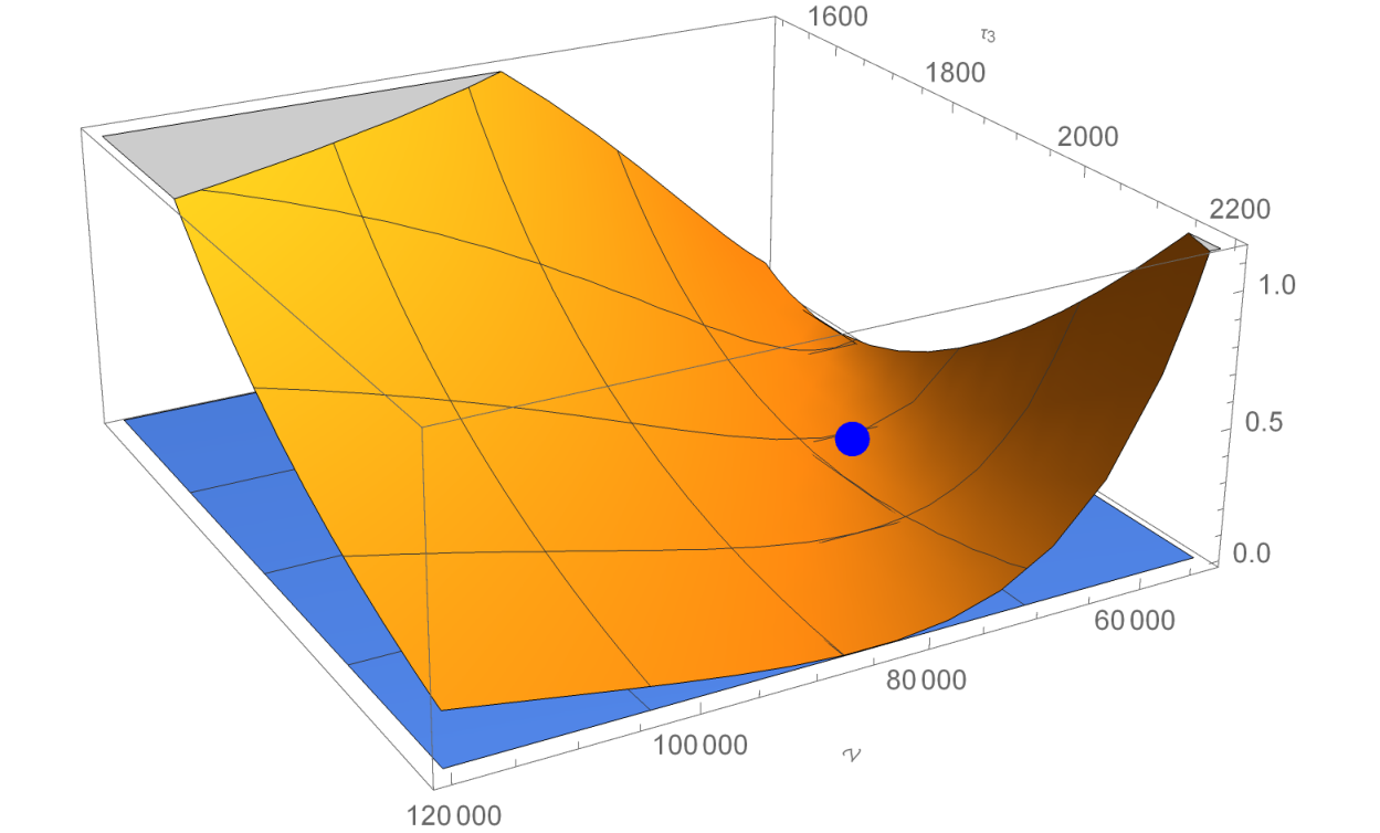
The potential (41) is plotted in figure 3 as a function of the volume for three values of the parameter . In figure 4 a three dimensional plot is shown where the minimum is depicted along and directions.
,
5 Probing the strong coupling regime
The approximations used in the previous sections were suitable to explore regions of the parameter space where the moduli are large and the exponential factors of the non-perturbative terms in the superpotential are suppressed. The analysis in this section will also be valid for regions of moduli values not much larger than where the non-perturbative corrections are substantially larger. To this end, a different approach will be followed in this section and the solutions of the flatness conditions (16,17) will be expressed in terms of the parameter and the modulus , namely:
| (46) |
where is shorthand for the solution. It should be remarked that, in contrast to the first case, these solutions of (21) are exact and no assumptions have been made. The only drawback of this parametrization is that the solutions of the minimization conditions are expressed in terms of implicit functions for all moduli fields and thus, it is more difficult to handle them analytically. Imposing the two conditions (46), the scalar potential takes the simple form
| (47) |
This potential encapsulates all the features of the potentials derived in the previous sections: the pure non-perturbative term , the perturbative one and a higher order mixing term . Minimization along the volume direction gives the value of at the minimum of the potential:
| (48) |
It was already pointed out in the previous sections that the F-term part implies always an AdS minimum and thus the D-terms are crucial for its uplifting to a dS vacuum. Including the D-term part (37), the total potential is written as:
| (49) |
where in the second line the from has been omitted. Minimizing (49) with respect to the modulus, its minimal value along is found to be:
| (50) |
Substitution of (50) into (49) yields,
| (51) |
Once a positive minimum along the volume direction is ensured, with a few more additional constraints on the parameter space, it can be shown that a minimum along all moduli directions is achievable. In figure 5 a characteristic case is plotted where the moduli fields acquire moderate values.

6 Concluding remarks
The cosmological predictions of effective theory models derived from string theory compactifications are the subject of intensive investigation. Among the primary and most important objectives towards this goal is the construction of string vacua with positive cosmological constant. In this work the combined effects of novel perturbative logarithmic string loop corrections in the Kähler potential, and non-perturbative contributions in the superpotential have been analyzed in the framework of type IIB string theory. In general, such quantum corrections are of key significance not merely for the existence of de Sitter (dS) minima but also for the (well known) moduli stabilization problem. Type IIB string theory and in particular its geometric variant, F-theory, are of great interest since they provide the necessary ingredients for a successful interpretation of these two important issues. Within this framework, a geometric configuration of three brane stacks intersecting each other is considered and three Kähler moduli are introduced whose imaginary parts determine the internal volume through .
The logarithmic terms involve the Kähler moduli and are induced from loop corrections when closed strings emitted from localized Einstein-Hilbert (EH) terms propagate through the codimension-two volume towards the seven-brane probes [31]. Such novel EH terms originate from the corrections of the effective ten-dimensional string action and appear only in four spacetime dimensions. The non-perturbative effects are assumed to be associated with gaugino condensation on the stacks and modify the superpotential with corrections of the usual exponential Kähler moduli dependence. The case of non-perturbative corrections where one or two Kähler moduli contribute has been worked out. In the large volume regime it has been found that the potential takes the generic simple form
where positive coefficients and the parameters -proportional to the Euler characteristic- and with the brane tension and the string coupling [31]. The term proportional to encapsulates perturbative contributions through the constants and the term combines positive contributions from D-terms and negative ones from non-perturbative corrections. The necessary conditions for Kähler moduli stabilization and dS minima are () and . It has been demonstrated in this article that a simultaneous solution for both problems can be guaranteed for a variety of appropriate flux choices and gaugino condensation parameters.
Finally, it should be noted that within the present geometric setup, there may exist charged matter fields associated with the excitations of open strings with their ends attached to brane stacks. Their scalar components may receive supersymmetric positive square masses from brane separation or Wilson lines, and non-supersymmetric contributions due to the presence of the worldvolume magnetic fields. With suitable conditions on various quantities such as magnetic fluxes and geometric characteristics (e.g. ratios of torii areas), all but a few masses-squared turn positive. In the simplest scenario it can be arranged that one tachyonic field arises from magnetised D7 brane identified with its orientifold image. In fact, its mass squared turns negative when the internal volume acquires a critical value. As a consequence, they induce specific contributions to the F- and D-terms of the effective potential. With these new ingredients, it has been shown [33] that this can play the rôle of the waterfall field, providing in this way an explicit string realization of the hybrid inflationary scenario.
Acknowledgments: “This research work was supported by the Hellenic Foundation for Research and Innovation (H.F.R.I.) under the “First Call for H.F.R.I. Research Projects to support Faculty members and Researchers and the procurement of high-cost research equipment grant” (Project Number: 2251)”. The work of V.B. is partially supported by the Research Committee of the University of Ioannina.
7 Appendix
7.1 The Potential with a single non-perturbative correction
The effective potential with a single non-perturbative correction has the following form:
| (52) |
Exchanging one modulus e.g. with the volume and minimizing for , (52) takes the form:
| (53) |
where
| (54) |
Next, minimization with respect to the , leads to the following equation:
| (55) |
For large and in the limit where the second term can be ignored, this equation takes the simple form and the solution is
| (56) |
The potential at the minimum is
| (57) |
Thus, it takes the previous form up to the factor , whereas . For large , and the potential (57) reduces to that of (6).
7.2 The F-term potential with two NP corrections
The exact form of the perturbative part of the F-term potential in section 3 is
Expanding in and , this takes the simplified form
| (58) |
The last approximated form (58) is the expression (27) in section 3.
The pure non-perturbative part is
Implementing the definitions , and making successively the substitutions
| (59) |
which follow from the solutions (23), this becomes
which is the form (28) of section 3.
Remarkably, this term has a volume dependence which is exactly the dependence of the D-term uplift in (6). For the regions where the approximation is valid, however, because the contribution of this term is negative and deepens the AdS vacuum.1111 11 Nonetheless, it will be seen that this term has the same power-law volume dependence with the positive D-term contributions and can be compensated by larger values of the parameter .
The mixing term of perturbative and non-perturbative corrections is a complicated function and can be elaborated in a similar manner.
7.3 The exact potential
In order to probe various regions of the parameter space, in the main text we have worked out several approximations of the F-term scalar potential. These constitute limiting cases of exact form given below:
where
Using the exact potential, all regions of the parameter space can be probed. For example, cases with comparable with cannot be examined in the approximations discussed so far. Here is a case with large . The following values of the parameters
| (60) |
are used to plot figure 6 with the exact .

References
- [1] C. Vafa, “The String landscape and the swampland,” hep-th/0509212.
- [2] G. Obied, H. Ooguri, L. Spodyneiko and C. Vafa, “De Sitter Space and the Swampland,” arXiv:1806.08362 [hep-th].
- [3] P. Agrawal, G. Obied, P. J. Steinhardt and C. Vafa, “On the Cosmological Implications of the String Swampland,” Phys. Lett. B 784 (2018) 271 [arXiv:1806.09718 [hep-th]].
- [4] U. H. Danielsson and T. Van Riet, “What if string theory has no de Sitter vacua?,” Int. J. Mod. Phys. D 27 (2018) no.12, 1830007 [arXiv:1804.01120 [hep-th]].
- [5] E. Palti, “The Swampland: Introduction and Review,” Fortsch. Phys. 67, no. 6, 1900037 (2019) [arXiv:1903.06239 [hep-th]].
- [6] M. van Beest, J. Calderón-Infante, D. Mirfendereski and I. Valenzuela, “Lectures on the Swampland Program in String Compactifications,” [arXiv:2102.01111 [hep-th]].
- [7] C. Roupec and T. Wrase, “de Sitter Extrema and the Swampland,” Fortsch. Phys. 67 (2019) no.1-2, 1800082 [arXiv:1807.09538 [hep-th]].
- [8] D. Andriot, “Tachyonic de Sitter solutions of 10d type II supergravities,” [arXiv:2101.06251 [hep-th]].
- [9] D. Andriot, P. Marconnet and T. Wrase, “Intricacies of classical de Sitter string backgrounds,” Phys. Lett. B 812 (2021), 136015 [arXiv:2006.01848 [hep-th]].
- [10] I. Basile and A. Platania, “Asymptotic Safety: Swampland or Wonderland?,” [arXiv:2107.06897 [hep-th]].
- [11] I. Basile and A. Platania, “String Tension between de Sitter vacua and Curvature Corrections,” [arXiv:2103.06276 [hep-th]].
- [12] D. Junghans, “Weakly Coupled de Sitter Vacua with Fluxes and the Swampland,” JHEP 03 (2019), 150 [arXiv:1811.06990 [hep-th]].
- [13] R. Blumenhagen, C. Kneissl and A. Makridou, “De Sitter Quantum Breaking, Swampland Conjectures and Thermal Strings,” [arXiv:2011.13956 [hep-th]].
- [14] S. Kachru, R. Kallosh, A. D. Linde and S. P. Trivedi, “De Sitter vacua in string theory,” Phys. Rev. D 68 (2003) 046005 [hep-th/0301240].
- [15] M. Cicoli, J. P. Conlon and F. Quevedo, “Systematics of String Loop Corrections in Type IIB Calabi-Yau Flux Compactifications,” JHEP 01 (2008), 052 [arXiv:0708.1873 [hep-th]].
- [16] J. Polchinski, “Brane/antibrane dynamics and KKLT stability,” [arXiv:1509.05710 [hep-th]].
- [17] Y. Hamada, A. Hebecker, G. Shiu and P. Soler, “Understanding KKLT from a 10d perspective,” JHEP 06 (2019), 019 [arXiv:1902.01410 [hep-th]].
- [18] F. Carta, J. Moritz and A. Westphal, “Gaugino condensation and small uplifts in KKLT,” JHEP 08 (2019), 141 [arXiv:1902.01412 [hep-th]].
- [19] R. Blumenhagen, D. Kläwer and L. Schlechter, “Swampland Variations on a Theme by KKLT,” JHEP 05 (2019), 152 [arXiv:1902.07724 [hep-th]].
- [20] M. Demirtas, M. Kim, L. Mcallister and J. Moritz, “Vacua with Small Flux Superpotential,” Phys. Rev. Lett. 124 (2020) no.21, 211603 [arXiv:1912.10047 [hep-th]].
- [21] R. Álvarez-García, R. Blumenhagen, M. Brinkmann and L. Schlechter, “Small Flux Superpotentials for Type IIB Flux Vacua Close to a Conifold,” [arXiv:2009.03325 [hep-th]].
- [22] I. Broeckel, M. Cicoli, A. Maharana, K. Singh and K. Sinha, “On the Search for Low ,” [arXiv:2108.04266 [hep-th]].
- [23] Y. Honma and H. Otsuka, “Small flux superpotential in F-theory compactifications,” Phys. Rev. D 103 (2021) no.12, 126022 [arXiv:2103.03003 [hep-th]].
- [24] K. Becker, M. Becker, M. Haack and J. Louis, “Supersymmetry breaking and alpha-prime corrections to flux induced potentials,” JHEP 0206 (2002) 060 [hep-th/0204254].
- [25] M. T. Grisaru, A. E. M. van de Ven and D. Zanon, “Four Loop beta Function for the N=1 and N=2 Supersymmetric Nonlinear Sigma Model in Two-Dimensions,” Phys. Lett. B 173 (1986), 423-428
- [26] I. Antoniadis, S. Ferrara, R. Minasian and K. S. Narain, “ couplings in M and type II theories on Calabi-Yau spaces,” Nucl. Phys. B 507 (1997) 571 [hep-th/9707013].
- [27] I. Antoniadis, R. Minasian, S. Theisen and P. Vanhove, “String loop corrections to the universal hypermultiplet,” Class. Quant. Grav. 20 (2003), 5079-5102 doi:10.1088/0264-9381/20/23/009 [arXiv:hep-th/0307268 [hep-th]].
- [28] M. B. Green and P. Vanhove, “D instantons, strings and M theory,” Phys. Lett. B 408 (1997) 122 [hep-th/9704145].
- [29] E. Kiritsis and B. Pioline, “On threshold corrections in IIb string theory and (p, q) string instantons,” Nucl. Phys. B 508, 509 (1997) [hep-th/9707018].
- [30] I. Antoniadis, Y. Chen and G. K. Leontaris, “Perturbative moduli stabilisation in type IIB/F-theory framework,” Eur. Phys. J. C 78 (2018) no.9, 766 [arXiv:1803.08941 [hep-th]].
- [31] I. Antoniadis, Y. Chen and G. K. Leontaris, “Logarithmic loop corrections, moduli stabilisation and de Sitter vacua in string theory,” JHEP 01 (2020), 149 [arXiv:1909.10525 [hep-th]].
- [32] I. Antoniadis, O. Lacombe and G. K. Leontaris, “Inflation near a metastable de Sitter vacuum from moduli stabilisation,” Eur. Phys. J. C 80 (2020) no.11, 1014 [arXiv:2007.10362 [hep-th]].
- [33] I. Antoniadis, O. Lacombe and G. K. Leontaris, “Hybrid inflation and waterfall field in string theory from D7-branes,” [arXiv:2109.03243 [hep-th]].
- [34] V. Basiouris and G. K. Leontaris, “Note on de Sitter vacua from perturbative and non-perturbative dynamics in type IIB/F-theory compactifications,” Phys. Lett. B 810 (2020), 135809 [arXiv:2007.15423 [hep-th]].
- [35] M. Cicoli, I. G. Etxebarria, F. Quevedo, A. Schachner, P. Shukla and R. Valandro, “The Standard Model Quiver in de Sitter String Compactifications,” [arXiv:2106.11964 [hep-th]].
- [36] J. J. Blanco-Pillado, C. P. Burgess, J. M. Cline, C. Escoda, M. Gomez-Reino, R. Kallosh, A. D. Linde and F. Quevedo, “Racetrack inflation,” JHEP 11 (2004), 063 [arXiv:hep-th/0406230 [hep-th]].
- [37] S. R. Coleman and E. J. Weinberg, “Radiative Corrections as the Origin of Spontaneous Symmetry Breaking,” Phys. Rev. D 7 (1973), 1888-1910
- [38] S. Gukov, C. Vafa and E. Witten, “CFT’s from Calabi-Yau four folds,” Nucl. Phys. B 584 (2000), 69-108 [erratum: Nucl. Phys. B 608 (2001), 477-478] [arXiv:hep-th/9906070 [hep-th]].
- [39] C. P. Burgess, C. Escoda and F. Quevedo, “Nonrenormalization of flux superpotentials in string theory,” JHEP 06 (2006), 044 [arXiv:hep-th/0510213 [hep-th]].
- [40] M. Bianchi, A. Collinucci and L. Martucci, “Magnetized E3-brane instantons in F-theory,” JHEP 12 (2011), 045 [arXiv:1107.3732 [hep-th]].
- [41] A. D. Linde, “Inflationary Cosmology,” Lect. Notes Phys. 738 (2008), 1-54 [arXiv:0705.0164 [hep-th]].
- [42] M. R. Douglas and S. Kachru, “Flux compactification,” Rev. Mod. Phys. 79 (2007), 733-796 [arXiv:hep-th/0610102 [hep-th]].
- [43] I. Antoniadis, R. Minasian and P. Vanhove, “Noncompact Calabi-Yau manifolds and localized gravity,” Nucl. Phys. B 648 (2003), 69-93 doi:10.1016/S0550-3213(02)00974-4 [arXiv:hep-th/0209030 [hep-th]].
- [44] F. Denef and M. R. Douglas, “Distributions of flux vacua,” JHEP 05 (2004), 072 [arXiv:hep-th/0404116 [hep-th]].
- [45] S. B. Giddings, S. Kachru and J. Polchinski, “Hierarchies from fluxes in string compactifications,” Phys. Rev. D 66 (2002), 106006 [arXiv:hep-th/0105097 [hep-th]].
- [46] K. Choi, A. Falkowski, H. P. Nilles, M. Olechowski and S. Pokorski, “Stability of flux compactifications and the pattern of supersymmetry breaking,” JHEP 11 (2004), 076 [arXiv:hep-th/0411066 [hep-th]].
- [47] T. W. Grimm, C. Li and E. Palti, “Infinite Distance Networks in Field Space and Charge Orbits,” JHEP 03 (2019), 016 [arXiv:1811.02571 [hep-th]].
- [48] T. W. Grimm, C. Li and I. Valenzuela, “Asymptotic Flux Compactifications and the Swampland,” JHEP 06 (2020), 009 [erratum: JHEP 01 (2021), 007] [arXiv:1910.09549 [hep-th]].
- [49] A. P. Braun and R. Valandro, “ flux, algebraic cycles and complex structure moduli stabilization,” JHEP 01 (2021), 207 [arXiv:2009.11873 [hep-th]].
- [50] F. Marchesano, D. Prieto and M. Wiesner, “F-theory flux vacua at large complex structure,” JHEP 08 (2021), 077 [arXiv:2105.09326 [hep-th]].
- [51] W. Schmid, “Variation of Hodge Structure: The Singularities of the Period Mapping,” Invent. Math. 22 (1973) 211-320.
- [52] I. Bena, J. Blåbäck, M. Graña and S. Lüst, “The Tadpole Problem,” [arXiv:2010.10519 [hep-th]].
- [53] S. Kachru, J. Pearson and H. L. Verlinde, “Brane / flux annihilation and the string dual of a nonsupersymmetric field theory,” JHEP 06 (2002), 021 [arXiv:hep-th/0112197 [hep-th]].
- [54] S. Ferrara, R. Kallosh and A. Linde, “Cosmology with Nilpotent Superfields,” JHEP 10 (2014), 143 [arXiv:1408.4096 [hep-th]].
- [55] D. V. Volkov and V. P. Akulov, “Is the Neutrino a Goldstone Particle?,” Phys. Lett. B 46 (1973), 109-110
- [56] M. Rocek, “Linearizing the Volkov-Akulov Model,” Phys. Rev. Lett. 41 (1978), 451-453 doi:10.1103/PhysRevLett.41.451
- [57] Z. Komargodski and N. Seiberg, “From Linear SUSY to Constrained Superfields,” JHEP 09 (2009), 066 [arXiv:0907.2441 [hep-th]].
- [58] I. Antoniadis, E. Dudas, D. M. Ghilencea and P. Tziveloglou, “Non-linear MSSM,” Nucl. Phys. B 841 (2010), 157-177 [arXiv:1006.1662 [hep-ph]].
- [59] C. P. Burgess, R. Kallosh and F. Quevedo, “De Sitter string vacua from supersymmetric D terms,” JHEP 10 (2003), 056 [arXiv:hep-th/0309187 [hep-th]].
- [60] M. Haack, D. Krefl, D. Lüst, A. Van Proeyen and M. Zagermann, “Gaugino Condensates and D-terms from D7-branes,” JHEP 01 (2007), 078 [arXiv:hep-th/0609211 [hep-th]].