跳到论文正文
W Papers独立论文阅读器 arXiv:2109.08397 论文正文 计算阅读时间 · 0%
引用这篇论文根据当前论文元数据生成,正式投稿前建议核对。


License: arXiv.org perpetual non-exclusive license
arXiv:2109.08397v1 [math-ph] 17 Sep 2021

Asymptotic analysis of random walks on ice and graphitePreprint: AIP/123-QED

Bernard Bercu Affiliation: Institut de Mathématiques de Bordeaux, Université de Bordeaux, UMR 5251, 351 Cours de la Libération, 33405 Talence cedex, France.    Fabien Montégut Email: fabien.montegut@math.univ-toulouse.fr. Affiliation: Institut de Mathématiques de Toulouse, Université de Toulouse, UMR 5219, 118 Route de Narbonne, 31062 Toulouse cedex, France.
August 11, 2026
Abstract

The purpose of this paper is to investigate the asymptotic behavior of random walks on three-dimensional crystal structures. We focus our attention on the 1​h1h structure of the ice and the 2​h2h structure of graphite. We establish the strong law of large numbers and the asymptotic normality for both random walks on ice and graphite. All our analysis relies on asymptotic results for multi-dimensional martingales.

Keywords: 
Random walk, Hexagonal lattice, Central limit theorem
MSC (2010) Primary: 60G50; Secondary: 60F05; 82C41

I Introduction

A wide variety of materials present a repeating symmetrical arrangement of their atoms, molecules or ions, known as crystal structures. Those underlying structures determine some physical properties such as the toughness, the porosity or even the conductivity of the materials. They can be looked further upon by studying the behavior of random walks in the crystal structures, see e.g. (BZ82) for a study of energy trapping in crystal structure or (Kovacik96) for the electrical conductivity of Cu-graphite composites. In particular, random walks are widely used to determine the diffusion of vacancies or point defects in crystals Koiwa.

Random walks represent a large class of Markov chains and several reference books Feller; Rudnick are devoted to the study of their properties, such as the probability of returning to their starting point, the shape of typical trajectories or their long-time behavior. Polya Polya was the first to observe the influence of the dimension of the lattice on their properties, as the simple random walk on ℤd\mathbb{Z}^{d} becomes transient when d≥3d\geq 3. The model of a non simple random walk on periodic lattice is quite convenient to study the properties of crystalline solids as stated in (Montroll).

Cubic crystal structures were previously studied in terms of random walks Garza or vacancy diffusions Bocquet, see also (deForcrand) and (GarzaHexa) for planar honeycomb lattices. However, to the best of our knowledge, three-dimensional hexagonal lattices still have to be considered. The goal of this paper is to investigate the asymptotic behavior of random walks in two hexagonal crystal structures in three dimensions, namely the 1​h1h structure of the ice and the 2​h2h structure of graphite. Both of them can be seen as sheets of infinite hexagonal plane lattices stacked on top of each other, where the way the consecutive sheets are stacked drastically changes the properties of the structure.

On the one hand, the properties of ice are theoretical and experimental research subjects since decades, see e.g. the pioneering works (Bradley57) or (DMS64). On the other hand, graphite composites finds many applications in a wide range of fields, see e.g. (Inagaki89) as well as the references therein, and its 2​h2h structure may be found in other materials Perevislov19. In both cases, understanding the asymptotic behavior of random walks in such structures is a key step in unveiling some of these materials properties.

Random walks on the two-dimensional hexagonal structure of the graphene has been described many times, especially in (Crescenzo19) where the authors studied the large deviation properties of the random walk, using a parity argument based on the structure of such lattice. Our purpose is to extend several results in (Crescenzo19) to the three-dimensional hexagonal structures we are interested in. In this paper, we assume that the transition probabilities are invariant by translating the unit cell of the crystal. Our goal is to establish the strong law of large numbers and the asymptotic normality of the random walk in both structures.

Our strategy is to separate the vertices of the lattice depending on their local geometry. In the simple case of the random walk on ice (RWI), there are only two different types of vertices. On the contrary, the random walk on the graphite (RWG) admits four different types of vertices and this situation is much more difficult to handle.

The paper is organized as follows: the definition and description of the random walks and their transition probabilities are given in Section 2. Section 3 is devoted to our main results. To be more precise, we establish the strong law of large numbers and the asymptotic normality for both RWI and RWG. The results concerning the RWI are proven in Section 4, while their counterparts for the RWG are postponed to Section 5. All our analysis relies on asymptotic results for multi-dimensional martingales. Finally, Section 6 contains concluding remarks and perspectives.

II Two possible structures

The two-dimensional hexagonal structure of the graphene was previously considered in (Crescenzo19) where two different kind of vertices 𝒱0\mathcal{V}_{0} and 𝒱1\mathcal{V}_{1} are represented in Figure 1 with white and black circles.

Refer to caption
Figure 1: Hexagonal structure of the graphene

In all the sequel, we shall focus our attention on two different type of structures. The first one corresponds to the 1​h1h structure of the ice. Sheets are stacked in such a way that the moving particle can always jump from one sheet to another one with small probability, as shown in Figure 2.

Refer to caption
Figure 2: Ice with 1​h1h structure.

One can observe that a particle located at a white vertex (resp. black vertex) is only allowed to jump to a white vertex (resp. black vertex). The set of vertices are denoted once again by 𝒱0\mathcal{V}_{0} and 𝒱1\mathcal{V}_{1} where for i=0,1i=0,1,

𝒱i={(a×(i+32k),a×(32k+3ℓ),h×n):k,ℓ,n∈ℤ}\mathcal{V}_{i}=\left\{\Bigl(a\times\Bigl(i+\frac{3}{2}k\Bigr),a\times\Bigl(\frac{\sqrt{3}}{2}k+\sqrt{3}\ell\Bigr),\ h\times n\Bigr)\ :\ k,\ell,n\in\mathbb{Z}\right\}

where aa stands for the distance between adjacent vertices located in the same sheet and hh stands for the distance between consecutive sheets of the ice. The index i=0i=0 if the vertex is white and the index i=1i=1 if the vertex is black.

The random walk on the ice with 1​h1h structure is as follows. At time zero, the particle starts at the origin S0=(0,0,0)S_{0}=(0,0,0). Afterwards, at time n≥0n\geq 0, assume that the position of the particle is given by Sn=(Xn,Yn,Zn)S_{n}=(X_{n},Y_{n},Z_{n}). Then, the particle can jump to an adjacent sheet with small probabilities, that is for i=0,1i=0,1 and for all (x,y,z)∈𝒱i(x,y,z)\in\mathcal{V}_{i},

ℙ[Sn+1=(xyz+h)|Sn=(xyz)]=αp\mathbb{P}\left[S_{n+1}=\left(\begin{array}[]{c}x\\ y\\ z+h\end{array}\right)\left|\ S_{n}=\left(\begin{array}[]{c}x\\ y\\ z\end{array}\right)\right.\right]=\alpha p (1)

while

ℙ[Sn+1=(xyz−h)|Sn=(xyz)]=(1−α)p\mathbb{P}\left[S_{n+1}=\left(\begin{array}[]{c}x\\ y\\ z-h\end{array}\right)\left|\ S_{n}=\left(\begin{array}[]{c}x\\ y\\ z\end{array}\right)\right.\right]=(1-\alpha)p (2)

where 0⩽p⩽10\leqslant p\leqslant 1 and 0<α<10<\alpha<1, the symmetrical case corresponding to α=1/2\alpha=1/2. Otherwise, if the particle remains on the same sheet, the transition probabilities are the same as those in (Crescenzo19), that is for i=0,1i=0,1, for all (x,y,z)∈𝒱i(x,y,z)\in\mathcal{V}_{i} and for j=0,1,2j=0,1,2,

ℙ[Sn+1=(x+a​cos⁡(23​j​π+i​π)y+a​sin⁡(23​j​π+i​π)z)|Sn=(xyz)]=pi,j\mathbb{P}\left[S_{n+1}=\left(\begin{array}[]{c}x+a\cos\bigl(\frac{2}{3}j\pi+i\pi\bigr)\\ y+a\sin\bigl(\frac{2}{3}j\pi+i\pi\bigr)\\ z\end{array}\right)\left|\ S_{n}=\left(\begin{array}[]{c}x\\ y\\ z\end{array}\right)\right.\right]=p_{i,j} (3)

where for i=0,1i=0,1,

∑j=02pi,j=1−p.\sum_{j=0}^{2}p_{i,j}=1-p.

The transition probabilities are represented in Figure 3. More precisely, if the particle is located in a vertex of 𝒱0\mathcal{V}_{0}, it can jump to the sheets above or below in a vertex of 𝒱0\mathcal{V}_{0} with small probabilities α​p\alpha p and (1−α)​p(1-\alpha)p respectively, or it can reach the three adjacent vertices of 𝒱1\mathcal{V}_{1} with probabilities p0,0p_{0,0}, p0,1p_{0,1} and p0,2p_{0,2}. By the same token, if the particle is located in a vertex of 𝒱1\mathcal{V}_{1}, it can jump to the sheets above or below in a vertex of 𝒱1\mathcal{V}_{1} with small probabilities α​p\alpha p and (1−α)​p(1-\alpha)p respectively, or it can reach the three adjacent vertices of 𝒱0\mathcal{V}_{0} with probabilities p1,0p_{1,0}, p1,1p_{1,1} and p1,2p_{1,2}.

Refer to caption
Figure 3: Transition probabilities for the 1​h1h structure of the ice.

A second type of structure we are interested in, is the 2​h2h structure of the graphite represented in Figure 4 where a particle located at a white vertex (resp. black vertex) can only jump to a black vertex (resp. white vertex). In other words, white vertices (resp. black vertices) of a given sheet are only connected to black vertices (resp. white vertices) of the graphite sheets just above or below.
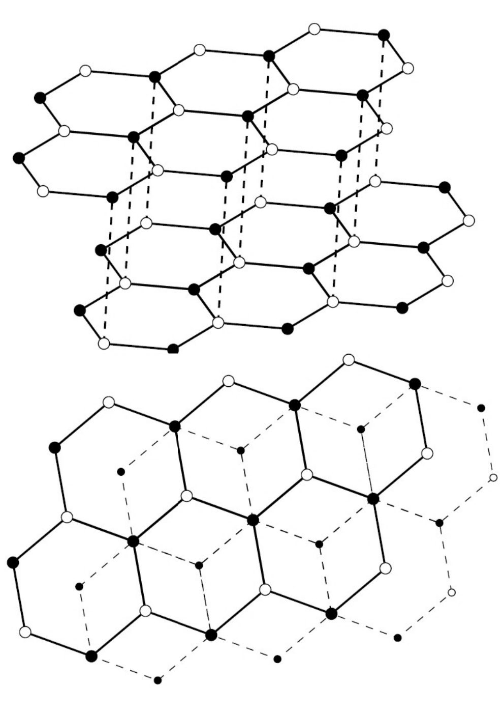
Refer to caption
Figure 4: Graphite with 2​h2h structure.

The set of vertices are now denoted by 𝒱0,0\mathcal{V}_{0,0}, 𝒱1,0\mathcal{V}_{1,0} and 𝒱0,1\mathcal{V}_{0,1}, 𝒱1,1\mathcal{V}_{1,1} where for i=0,1i=0,1 and j=0,1j=0,1,

𝒱i,j={(a×((−1)i+1\displaystyle\mathcal{V}_{i,j}\!=\!\Bigg\{\Biggl(a\times\Bigl((-1)^{i+1} OPEN𝟙𝕛=𝟙+𝟛𝟚​𝕜),𝕒×(𝟛𝟚​𝕜+𝟛​ℓ),\displaystyle\openone_{j=1}+\frac{3}{2}k\Bigr),a\times\Bigl(\frac{\sqrt{3}}{2}k+\sqrt{3}\ell\Bigr),
h×(2n+𝟙𝕚≠𝕛))with𝕜,ℓ,𝕟∈ℤ}\displaystyle h\times(2n+\openone_{i\neq j})\Biggr)\ \text{with}\ k,\ell,n\in\mathbb{Z}\Bigg\}

where as before aa is the distance between adjacent vertices located in the same sheet and hh is the distance between consecutive sheets of graphene. The index i=0i=0 if the vertex is white and i=1i=1 if the vertex is black (which refers to the horizontal local neighborhood), while the index j=0j=0 if the particle can move to an adjacent sheet from this vertex and j=1j=1 otherwise. The main difference with the 1​h1h structure of the ice is that here the particle does not always have the possibility to jump to an adjacent sheet.

The random walk on the graphite with 2​h2h structure is as follows. At time zero, the particle starts at the origin S0=(0,0,0)S_{0}=(0,0,0). Afterwards, at time n≥0n\geq 0, assume that the position of the particle is given by Sn=(Xn,Yn,Zn)S_{n}=(X_{n},Y_{n},Z_{n}). Then, for i=0,1i=0,1, if the particle is located in 𝒱i,0\mathcal{V}_{i,0}, it has the possibility to jump to an adjacent sheet with small probabilities, that is for i=0,1i=0,1 and for all (x,y,z)∈𝒱i,0(x,y,z)\in\mathcal{V}_{i,0},

ℙ[Sn+1=(xyz+h)|Sn=(xyz)]=αp\mathbb{P}\left[S_{n+1}=\left(\begin{array}[]{c}x\\ y\\ z+h\end{array}\right)\left|\ S_{n}=\left(\begin{array}[]{c}x\\ y\\ z\end{array}\right)\right.\right]=\alpha p (4)

while

ℙ[Sn+1=(xyz−h)|Sn=(xyz)]=(1−α)p\mathbb{P}\left[S_{n+1}=\left(\begin{array}[]{c}x\\ y\\ z-h\end{array}\right)\left|\ S_{n}=\left(\begin{array}[]{c}x\\ y\\ z\end{array}\right)\right.\right]=(1-\alpha)p (5)

where 0⩽p⩽10\leqslant p\leqslant 1 and 0<α<10<\alpha<1, the symmetrical case corresponding to α=1/2\alpha=1/2. Otherwise, for i=0,1i=0,1, if the particle is located in 𝒱i,0\mathcal{V}_{i,0} and it remains on the same sheet, the transition probabilities are given for all (x,y,z)∈𝒱i,0(x,y,z)\in\mathcal{V}_{i,0} and for k=0,1,2k=0,1,2, by

ℙ[Sn+1=(x+a​cos⁡(23​k​π+i​π)y+a​sin⁡(23​k​π+i​π)z)|Sn=(xyz)]=pi,0,k\mathbb{P}\left[S_{n+1}=\left(\begin{array}[]{c}x+a\cos\bigl(\frac{2}{3}k\pi+i\pi\bigr)\\ y+a\sin\bigl(\frac{2}{3}k\pi+i\pi\bigr)\\ z\end{array}\right)\left|\ S_{n}=\left(\begin{array}[]{c}x\\ y\\ z\end{array}\right)\right.\right]=p_{i,0,k} (6)

where for i=0,1i=0,1,

∑k=02pi,0,k=1−p.\sum_{k=0}^{2}p_{i,0,k}=1-p.

Finally, for i=0,1i=0,1, if the particle is located in 𝒱i,1\mathcal{V}_{i,1}, the transition probabilities are the same as those in (Crescenzo19), that is for i=0,1i=0,1, for all (x,y,z)∈𝒱i,1(x,y,z)\in\mathcal{V}_{i,1} and for k=0,1,2k=0,1,2,

ℙ[Sn+1=(x+a​cos⁡(23​k​π+i​π)y+a​sin⁡(23​k​π+i​π)z)|Sn=(xyz)]=pi,1,k\mathbb{P}\left[S_{n+1}=\left(\begin{array}[]{c}x+a\cos\bigl(\frac{2}{3}k\pi+i\pi\bigr)\\ y+a\sin\bigl(\frac{2}{3}k\pi+i\pi\bigr)\\ z\end{array}\right)\left|\ S_{n}=\left(\begin{array}[]{c}x\\ y\\ z\end{array}\right)\right.\right]=p_{i,1,k}

where for i=0,1i=0,1,

∑k=02pi,1,k=1.\sum_{k=0}^{2}p_{i,1,k}=1.

As it was previously done for the 1​h1h structure of the ice, the transition probabilities for the 2​h2h structure of the graphite are given in Figure 5.

Refer to caption
Figure 5: Transition probabilities for the 2​h2h structure of the graphite.

The goal of this paper is to investigate the asymptotic behavior of three-dimensional RWI and RWG with this two different type of structures. Figures  6 and  7 shows two trajectories of length n=10 000n=10\,000 of the RWI and RWG, respectively. The distance aa between adjacent vertices and the distance hh between consecutive sheets are given by a=1a=1 and h=1h=1, while the probability to jump to an adjacent sheet p=1/5p=1/5, α=1/2\alpha=1/2 and the transitions probabilities are given, for i=0,1i=0,1 and j=0,1,2j=0,1,2, by

pi,j=13​(1−p).p_{i,j}=\frac{1}{3}(1-p).
Refer to caption
Figure 6: Trajectory of the three-dimensional RWI.
Refer to caption
Figure 7: Trajectory of the three-dimensional RWG.

III Main results

Our first result concerns the strong law of large numbers for the random walk on ice structure. Let μ\mu be the mean vector defined by

μ=(μ1μ2μ3)\mu=\begin{pmatrix}\mu_{1}\\ \mu_{2}\\ \mu_{3}\end{pmatrix} (7)

with

μ1\displaystyle\mu_{1} =\displaystyle= 3​a4​(−u0+u1),\displaystyle\frac{3a}{4}\Bigl(-u_{0}+u_{1}\Bigr),
μ2\displaystyle\mu_{2} =\displaystyle= a​34​(v0−v1),\displaystyle\frac{a\sqrt{3}}{4}\Bigl(v_{0}-v_{1}\Bigr),
μ3\displaystyle\mu_{3} =\displaystyle= h​p​(2​α−1),\displaystyle\Big.hp(2\alpha-1),

where for i=0,1i=0,1, ui=pi,1+pi,2u_{i}=p_{i,1}+p_{i,2} and vi=pi,1−pi,2v_{i}=p_{i,1}-p_{i,2}.

Theorem III.1

For the RWI, we have the almost sure convergence

limn→∞1n​Sn=μa.s.\lim_{n\rightarrow\infty}\frac{1}{n}S_{n}=\mu\hskip 28.45274pt\text{a.s.} (8)

More precisely,

‖1n​Sn−μ‖2=O⁡(log⁡nn)a.s.\Bigl\|\frac{1}{n}S_{n}-\mu\Bigr\|^{2}=O\Bigl(\frac{\log n}{n}\Bigr)\hskip 28.45274pt\text{a.s.} (9)

Our second result is devoted to the asymptotic normality for the random walk on ice structure. For this purpose, denote

σ2=(σ12σ1,20σ1,2σ22000σ32)\sigma^{2}=\begin{pmatrix}\sigma^{2}_{1}&\sigma_{1,2}&0\\ \sigma_{1,2}&\sigma^{2}_{2}&0\\ 0&0&\sigma^{2}_{3}\end{pmatrix} (10)

where

σ12\displaystyle\sigma^{2}_{1} =a2​(p⁡(1−p)+38​(3−4​p)​(u0+u1)−98​(u02+u12)),\displaystyle=a^{2}\Bigl(p(1-p)+\frac{3}{8}(3-4p)\bigl(u_{0}+u_{1}\bigr)-\frac{9}{8}\bigl(u_{0}^{2}+u_{1}^{2}\bigr)\Bigr),
σ22\displaystyle\sigma^{2}_{2} =3​a28​((u0+u1)−(v02+v12)),\displaystyle=\frac{3a^{2}}{8}\Bigl(\bigl(u_{0}+u_{1}\bigr)-\bigl(v_{0}^{2}+v_{1}^{2}\bigr)\Bigr),
σ32\displaystyle\sigma^{2}_{3} =h2​p​(1−p​(2​α−1)2),\displaystyle=h^{2}p\Bigl(1-p\bigl(2\alpha-1\bigr)^{2}\Bigr),
σ1,2\displaystyle\sigma_{1,2} =a2​38​((−3+2​p)​(v0+v1)+3​(u0​v0+u1​v1)).\displaystyle=\frac{a^{2}\sqrt{3}}{8}\Bigl(\bigl(-3+2p\bigr)\bigl(v_{0}+v_{1}\bigr)+3\bigl(u_{0}v_{0}+u_{1}v_{1}\bigr)\Bigr).

In addition, let

θ=(θ1θ20)\theta=\begin{pmatrix}\theta_{1}\\ \theta_{2}\\ 0\end{pmatrix} (11)

with

θ1\displaystyle\theta_{1} =\displaystyle= a⁡((1−p)−34​(u0+u1)),\displaystyle a\Bigl((1-p)-\frac{3}{4}(u_{0}+u_{1})\Bigr),
θ2\displaystyle\theta_{2} =\displaystyle= 3​a4​(v0+v1).\displaystyle\frac{\sqrt{3}a}{4}\bigl(v_{0}+v_{1}\bigr).
Theorem III.2

For the RWI, we have the asymptotic normality

1n​(Sn−n​μ)⟶ℒ𝒩⁡(0,Γ)\frac{1}{\sqrt{n}}\bigl(S_{n}-n\mu\bigr)\mathrel{\mathop{\kern 0.0pt\longrightarrow}\limits^{{\mbox{\calcal L}}}}\mathcal{N}\left(0,\Gamma\right) (12)

where the covariance matrix Γ\Gamma is given by Γ=σ2\Gamma=\sigma^{2} if p=1p=1, whereas if 0≤p<10\leq p<1,

Γ=σ2−(p1−p)​θ​θT.\Gamma=\sigma^{2}-\Bigl(\frac{p}{1-p}\Bigr)\theta\theta^{T}. (13)

Our third result deals with the strong law of large numbers for the random walk on graphite structure. Denote by μ\mu and mm the mean vectors

μ=(μ1μ2μ3)andm=(m1m2m3)\mu=\begin{pmatrix}\mu_{1}\\ \mu_{2}\\ \mu_{3}\end{pmatrix}\hskip 28.45274pt\text{and}\hskip 28.45274ptm=\begin{pmatrix}m_{1}\\ m_{2}\\ m_{3}\end{pmatrix} (14)

with

μ1\displaystyle\mu_{1} =\displaystyle= 3​a8​(−(u0,0+u0,1)+(u1,0+u1,1)),\displaystyle\frac{3a}{8}\Bigl(-(u_{0,0}+u_{0,1})+(u_{1,0}+u_{1,1})\Bigr),
μ2\displaystyle\mu_{2} =\displaystyle= a​38​((v0,0+v0,1)−(v1,0+v1,1)),\displaystyle\frac{a\sqrt{3}}{8}\Bigl((v_{0,0}+v_{0,1})-(v_{1,0}+v_{1,1})\Bigr),
μ3\displaystyle\mu_{3} =\displaystyle= h​p2​(2​α−1)\displaystyle\frac{hp}{2}(2\alpha-1)

and

m1\displaystyle m_{1} =\displaystyle= 3​a8​(−(u0,0−u0,1)+(u1,0−u1,1)),\displaystyle\frac{3a}{8}\Bigl(-(u_{0,0}-u_{0,1})+(u_{1,0}-u_{1,1})\Bigr),
m2\displaystyle m_{2} =\displaystyle= a​38​((v0,0−v0,1)−(v1,0−v1,1)),\displaystyle\frac{a\sqrt{3}}{8}\Bigl((v_{0,0}-v_{0,1})-(v_{1,0}-v_{1,1})\Bigr),
m3\displaystyle m_{3} =\displaystyle= h​p2​(2​α−1)\displaystyle\frac{hp}{2}(2\alpha-1)

where for i,j=0,1i,j=0,1, ui,j=pi,j,1+pi,j,2u_{i,j}=p_{i,j,1}+p_{i,j,2} and vi,j=pi,j,1−pi,j,2v_{i,j}=p_{i,j,1}-p_{i,j,2}. For the sake of clarity, we have chosen to keep the same notation for the mean vector μ\mu in both hexagonal structures. We shall also make use of the vectors θ\theta and ρ\rho defined by

θ=(θ1θ20)andρ=(ρ1ρ20)\theta=\begin{pmatrix}\theta_{1}\\ \theta_{2}\\ 0\end{pmatrix}\hskip 28.45274pt\text{and}\hskip 28.45274pt\rho=\begin{pmatrix}\rho_{1}\\ \rho_{2}\\ 0\end{pmatrix} (15)

with

θ1\displaystyle\theta_{1} =\displaystyle= a⁡((1−p2)−38​((u0,0+u0,1)+(u1,0+u1,1))),\displaystyle a\Bigl(\Bigl(1-\frac{p}{2}\Bigr)-\frac{3}{8}\Bigl((u_{0,0}+u_{0,1})+(u_{1,0}+u_{1,1})\Bigr)\Bigr),
θ2\displaystyle\theta_{2} =\displaystyle= a​38​((v0,0+v0,1)+(v1,0+v1,1)),\displaystyle\frac{a\sqrt{3}}{8}\Bigl((v_{0,0}+v_{0,1})+(v_{1,0}+v_{1,1})\Bigr),
ρ1\displaystyle\rho_{1} =\displaystyle= a⁡(−p2−38​((u0,0−u0,1)+(u1,0−u1,1))),\displaystyle a\Bigl(-\frac{p}{2}-\frac{3}{8}\Bigl((u_{0,0}-u_{0,1})+(u_{1,0}-u_{1,1})\Bigr)\Bigr),
ρ2\displaystyle\rho_{2} =\displaystyle= a​38​((v0,0−v0,1)+(v1,0−v1,1)).\displaystyle\frac{a\sqrt{3}}{8}\Bigl((v_{0,0}-v_{0,1})+(v_{1,0}-v_{1,1})\Bigr).
Theorem III.3

For the RWG with p>0p>0, we have the almost sure convergence

limn→∞1n​Sn=μ+(p2−p)​ma.s.\lim_{n\rightarrow\infty}\frac{1}{n}S_{n}=\mu+\Bigl(\frac{p}{2-p}\Bigr)m\hskip 28.45274pt\text{a.s.} (16)

More precisely,

‖1n​Sn−μ−(p2−p)​m‖2=O⁡(log⁡nn)a.s.\Bigl\|\frac{1}{n}S_{n}-\mu-\Bigl(\frac{p}{2-p}\Bigr)m\Bigr\|^{2}=O\Bigl(\frac{\log n}{n}\Bigr)\hskip 28.45274pt\text{a.s.} (17)
Remark III.1

In the special case where p=0p=0, the limiting value in (16) and (17) changes to μ+ρ\mu+\rho,

limn→∞1n​Sn=μ+ρa.s.\lim_{n\rightarrow\infty}\frac{1}{n}S_{n}=\mu+\rho\hskip 28.45274pt\text{a.s.} (18)

and

‖1n​Sn−μ−ρ‖2=O⁡(log⁡nn)a.s.\Bigl\|\frac{1}{n}S_{n}-\mu-\rho\Bigr\|^{2}=O\Bigl(\frac{\log n}{n}\Bigr)\hskip 28.45274pt\text{a.s.} (19)

If we denote u0=u0,0u_{0}=u_{0,0}, u1=u1,1u_{1}=u_{1,1} and v0=v0,0v_{0}=v_{0,0}, v1=v1,1v_{1}=v_{1,1}, one can immediately see that the almost sure convergences (8) and (18) are of course the same in the case p=0p=0.

Our fourth result is dedicated to the asymptotic normality for the random walk on the graphene. To this end, let

ζ=(00h​p​(2​α−1)).\zeta=\begin{pmatrix}0\\ 0\\ hp(2\alpha-1)\end{pmatrix}. (20)

Moreover, denote

σ2=(σ12σ1,2σ1,3σ1,2σ22σ2,3σ1,3σ2,3σ32)andγ=(γ1γ4γ6γ4γ2γ5γ6γ5γ3)\sigma^{2}=\begin{pmatrix}\sigma^{2}_{1}&\sigma_{1,2}&\sigma_{1,3}\\ \sigma_{1,2}&\sigma^{2}_{2}&\sigma_{2,3}\\ \sigma_{1,3}&\sigma_{2,3}&\sigma^{2}_{3}\end{pmatrix}\hskip 28.45274pt\text{and}\hskip 28.45274pt\gamma=\begin{pmatrix}\gamma_{1}&\gamma_{4}&\gamma_{6}\\ \gamma_{4}&\gamma_{2}&\gamma_{5}\\ \gamma_{6}&\gamma_{5}&\gamma_{3}\end{pmatrix} (21)

where

σ12\displaystyle\sigma^{2}_{1} =a24​(2​p​(1−p)+94​(s0,0+s1,0+s0,1+s1,1)−3​p​(u0,0+u1,0)),\displaystyle=\frac{a^{2}}{4}\Bigl(2p(1-p)+\frac{9}{4}\bigl(s_{0,0}+s_{1,0}+s_{0,1}+s_{1,1}\bigr)-3p\bigl(u_{0,0}+u_{1,0}\bigr)\Bigr),
σ22\displaystyle\sigma^{2}_{2} =3​a216​((u0,0+u1,0+u0,1+u1,1)−(v0,02+v1,02+v0,12+v1,12)),\displaystyle=\frac{3a^{2}}{16}\Bigl(\bigl(u_{0,0}+u_{1,0}+u_{0,1}+u_{1,1}\bigr)-\bigl(v_{0,0}^{2}+v_{1,0}^{2}+v_{0,1}^{2}+v_{1,1}^{2}\bigr)\Bigr),
σ32\displaystyle\sigma^{2}_{3} =h2​p2​(1−p​(2​α−1)2),\displaystyle=\frac{h^{2}p}{2}\Bigl(1-p(2\alpha-1)^{2}\Bigr),
σ1,2\displaystyle\sigma_{1,2} =a2​316​(3​(t0,0+t1,0+t0,1+t1,1)+2​p​(v0,0+v1,0)),\displaystyle=\frac{a^{2}\sqrt{3}}{16}\Bigl(3\bigl(t_{0,0}+t_{1,0}+t_{0,1}+t_{1,1}\bigr)+2p\bigl(v_{0,0}+v_{1,0}\bigr)\Bigr),
σ2,3\displaystyle\sigma_{2,3} =−a​h​38​(p⁡(2​α−1)​(v0,0+v1,0)),\displaystyle=\frac{-ah\sqrt{3}}{8}\Bigl(p(2\alpha-1)\bigl(v_{0,0}+v_{1,0}\bigr)\Bigr),
σ1,3\displaystyle\sigma_{1,3} =a​h8​(−4​p​(1−p)​(2​α−1)+3​p​(2​α−1)​(u0,0+u1,0)),\displaystyle=\frac{ah}{8}\Bigl(-4p(1-p)(2\alpha-1)+3p(2\alpha-1)\bigl(u_{0,0}+u_{1,0}\bigr)\Bigr),

and

γ1\displaystyle\gamma_{1} =a24​(2​p​(1−p)+94​(s0,0+s1,0−s0,1−s1,1)−3​p​(u0,0+u1,0)),\displaystyle=\frac{a^{2}}{4}\Bigl(2p(1-p)+\frac{9}{4}\bigl(s_{0,0}+s_{1,0}-s_{0,1}-s_{1,1}\bigr)-3p\bigl(u_{0,0}+u_{1,0}\bigr)\Bigr),
γ2\displaystyle\gamma_{2} =3​a216​((u0,0+u1,0−u0,1−u1,1)−(v0,02+v1,02−v0,12−v1,12)),\displaystyle=\frac{3a^{2}}{16}\Bigl(\bigl(u_{0,0}+u_{1,0}-u_{0,1}-u_{1,1}\bigr)-\bigl(v_{0,0}^{2}+v_{1,0}^{2}-v_{0,1}^{2}-v_{1,1}^{2}\bigr)\Bigr),
γ3\displaystyle\gamma_{3} =h2​p2​(1−p​(2​α−1)2),\displaystyle=\frac{h^{2}p}{2}\Bigl(1-p(2\alpha-1)^{2}\Bigr),
γ4\displaystyle\gamma_{4} =a2​316​(3​(t0,0+t1,0−t0,1−t1,1)+2​p​(v0,0+v1,0)),\displaystyle=\frac{a^{2}\sqrt{3}}{16}\Bigl(3\bigl(t_{0,0}+t_{1,0}-t_{0,1}-t_{1,1}\bigr)+2p\bigl(v_{0,0}+v_{1,0}\bigr)\Bigr),
γ5\displaystyle\gamma_{5} =−a​h​38​(p⁡(2​α−1)​(v0,0+v1,0)),\displaystyle=\frac{-ah\sqrt{3}}{8}\Bigl(p(2\alpha-1)\bigl(v_{0,0}+v_{1,0}\bigr)\Bigr),
γ6\displaystyle\gamma_{6} =a​h8​(−4​p​(1−p)​(2​α−1)+3​p​(2​α−1)​(u0,0+u1,0)),\displaystyle=\frac{ah}{8}\Bigl(-4p(1-p)(2\alpha-1)+3p(2\alpha-1)\bigl(u_{0,0}+u_{1,0}\bigr)\Bigr),

with for all i=0,1i=0,1 and j=0,1j=0,1, si,j=ui,j​(1−ui,j)s_{i,j}=u_{i,j}(1-u_{i,j}) and ti,j=vi,j​(ui,j−1){t_{i,j}=v_{i,j}(u_{i,j}-1)}.

Theorem III.4

For the RWG with p>0p>0, we have the asymptotic normality

1n​(Sn−n​μ−n⁡(p2−p)​m)⟶ℒ𝒩⁡(0,Γ)\frac{1}{\sqrt{n}}\bigl(S_{n}-n\mu-n\Bigl(\frac{p}{2-p}\Bigr)m\bigr)\mathrel{\mathop{\kern 0.0pt\longrightarrow}\limits^{{\mbox{\calcal L}}}}\mathcal{N}\left(0,\Gamma\right) (22)

where the covariance matrix Γ\Gamma is given by

Γ\displaystyle\Gamma =σ2+p2−p​γ+2(2−p)2​((ζ−p​μ)​mT+m​(ζ−p​μ)T)\displaystyle=\sigma^{2}+\frac{p}{2-p}\gamma+\frac{2}{(2-p)^{2}}\Bigl(\bigl(\zeta-p\mu\bigr)m^{T}+m\bigl(\zeta-p\mu\bigr)^{T}\Bigr)
−4​p(2−p)3​m​mT+22−p​(θ​ρT+ρ​θT)+4p⁡(2−p)​ρ​ρT.\displaystyle\hskip 14.22636pt-\frac{4p}{(2-p)^{3}}mm^{T}+\frac{2}{2-p}\bigl(\theta\rho^{T}+\rho\theta^{T}\bigr)+\frac{4}{p(2-p)}\rho\rho^{T}. (23)
Remark III.2

In the special case where p=0p=0, we find that

1n​(Sn−n⁡(μ+ρ))⟶ℒ𝒩⁡(0,σ2+δ)\frac{1}{\sqrt{n}}\bigl(S_{n}-n(\mu+\rho)\bigr)\mathrel{\mathop{\kern 0.0pt\longrightarrow}\limits^{{\mbox{\calcal L}}}}\mathcal{N}\left(0,\sigma^{2}+\delta\right) (24)

where the matrix δ\delta is defined in (61). One can also observe that the asymptotic variances in (12) and (24) coincide in the case p=0p=0.

IV Proofs for the RWI

Proof of Theorem III.1. In order to prove the almost sure convergence (8), denote by (ξn)(\xi_{n}) the increments of the RWI. Then, the position of the RWI is given, for all n≥0n\geq 0, by

Sn+1=Sn+ξn+1=∑k=1n+1ξkS_{n+1}=S_{n}+\xi_{n+1}=\sum_{k=1}^{n+1}\xi_{k} (25)

where

ξn+1=(Xn+1−XnYn+1−YnZn+1−Zn).\xi_{n+1}=\begin{pmatrix}X_{n+1}-X_{n}\\ Y_{n+1}-Y_{n}\\ Z_{n+1}-Z_{n}\end{pmatrix}.

Let (ℱn)(\mathcal{F}_{n}) be the natural filtration associated with the RWI, that is ℱn=σ⁡(ξ1,…,ξn)\mathcal{F}_{n}=\sigma\big(\xi_{1},\dots,\xi_{n}\big). We have for all n≥0n\geq 0, 𝔼⁡[ξn+1|ℱn]=𝔼⁡[ξn+1|Sn∈𝒱0]​𝟙𝕊𝕟∈𝒱𝟘+𝔼⁡[ξ𝕟+𝟙|𝕊𝕟∈𝒱𝟙]​𝟙𝕊𝕟∈𝒱𝟙\mathbb{E}[\xi_{n+1}|\mathcal{F}_{n}]=\mathbb{E}[\xi_{n+1}|S_{n}\in\mathcal{V}_{0}]\openone_{S_{n}\in\mathcal{V}_{0}}+\mathbb{E}[\xi_{n+1}|S_{n}\in\mathcal{V}_{1}]\openone_{S_{n}\in\mathcal{V}_{1}}. Hence, it follows from (1), (2) and (3) that

𝔼⁡[ξn+1|ℱn]=(a⁡(p0,0−12​(p0,1+p0,2))a​32​(p0,1−p0,2)h​p​(2​α−1))​𝟙𝕊𝕟∈𝒱𝟘\displaystyle\mathbb{E}[\xi_{n+1}|\mathcal{F}_{n}]\!=\!\begin{pmatrix}a\bigl(p_{0,0}-\frac{1}{2}(p_{0,1}+p_{0,2})\bigr)\\ \frac{a\sqrt{3}}{2}\bigl(p_{0,1}-p_{0,2}\bigr)\\ hp(2\alpha-1)\end{pmatrix}\!\openone_{S_{n}\in\mathcal{V}_{0}}
+(a⁡(−p1,0+12​(p1,1+p1,2))a​32​(p1,2−p1,1)h​p​(2​α−1))​𝟙𝕊𝕟∈𝒱𝟙\displaystyle\!+\!\begin{pmatrix}a\bigl(-p_{1,0}+\frac{1}{2}(p_{1,1}+p_{1,2})\bigr)\\ \frac{a\sqrt{3}}{2}\bigl(p_{1,2}-p_{1,1}\bigr)\\ hp(2\alpha-1)\end{pmatrix}\!\openone_{S_{n}\in\mathcal{V}_{1}} .

For i=0,1i=0,1, denote ui=pi,1+pi,2u_{i}=p_{i,1}+p_{i,2} and vi=pi,1−pi,2v_{i}=p_{i,1}-p_{i,2}. We clearly have for i=0,1i=0,1, pi,0=1−p−uip_{i,0}=1-p-u_{i}. Consequently, 𝔼⁡[ξn+1|ℱn]\mathbb{E}[\xi_{n+1}|\mathcal{F}_{n}] reduces to

𝔼⁡[ξn+1|ℱn]=(μ+θ)​𝟙𝕊𝕟∈𝒱𝟘+(μ−θ)​𝟙𝕊𝕟∈𝒱𝟙=μ+θ​ε𝕟\mathbb{E}[\xi_{n+1}|\mathcal{F}_{n}]=(\mu+\theta)\openone_{S_{n}\in\mathcal{V}_{0}}+(\mu-\theta)\openone_{S_{n}\in\mathcal{V}_{1}}=\mu+\theta\varepsilon_{n} (26)

where εn\varepsilon_{n} stands for the random variable

εn=𝟙𝕊𝕟∈𝒱𝟘−𝟙𝕊𝕟∈𝒱𝟙\varepsilon_{n}=\openone_{S_{n}\in\mathcal{V}_{0}}-\openone_{S_{n}\in\mathcal{V}_{1}} (27)

and the vectors μ\mu and θ\theta are given by (7) and (11). Moreover, we have for all n≥0n\geq 0, 𝔼⁡[ξn+1​ξn+1T|ℱn]=𝔼⁡[ξn+1​ξn+1T|Sn∈𝒱0]​𝟙𝕊𝕟∈𝒱𝟘+𝔼⁡[ξ𝕟+𝟙​ξ𝕟+𝟙𝕋|𝕊𝕟∈𝒱𝟙]​𝟙𝕊𝕟∈𝒱𝟙\mathbb{E}[\xi_{n+1}\xi_{n+1}^{T}|\mathcal{F}_{n}]=\mathbb{E}[\xi_{n+1}\xi_{n+1}^{T}|S_{n}\in\mathcal{V}_{0}]\openone_{S_{n}\in\mathcal{V}_{0}}+\mathbb{E}[\xi_{n+1}\xi_{n+1}^{T}|S_{n}\in\mathcal{V}_{1}]\openone_{S_{n}\in\mathcal{V}_{1}}. We obtain once again from (1), (2) and (3) that

𝔼⁡[ξn+1​ξn+1T|ℱn]=\displaystyle\mathbb{E}[\xi_{n+1}\xi_{n+1}^{T}|\mathcal{F}_{n}]=
(a2​(p0,0+14​(p0,1+p0,2))−a2​34​(p0,1−p0,2)0−a2​34​(p0,1−p0,2)3​a24​(p0,1+p0,2)000h2​p)​𝟙𝕊𝕟∈𝒱𝟘\displaystyle\begin{pmatrix}a^{2}\bigl(p_{0,0}+\frac{1}{4}(p_{0,1}+p_{0,2})\bigr)&-\frac{a^{2}\sqrt{3}}{4}\bigl(p_{0,1}-p_{0,2}\bigr)&0\\ -\frac{a^{2}\sqrt{3}}{4}\bigl(p_{0,1}-p_{0,2}\bigr)&\frac{3a^{2}}{4}\bigl(p_{0,1}+p_{0,2}\bigr)&0\\ 0&0&h^{2}p\end{pmatrix}\openone_{S_{n}\in\mathcal{V}_{0}}
+(a2​(p1,0+14​(p1,1+p1,2))−a2​34​(p1,1−p1,2)0−a2​34​(p1,1−p1,2)3​a24​(p1,1+p1,2)000h2​p)​𝟙𝕊𝕟∈𝒱𝟙.\displaystyle+\begin{pmatrix}a^{2}\bigl(p_{1,0}+\frac{1}{4}(p_{1,1}+p_{1,2})\bigr)&-\frac{a^{2}\sqrt{3}}{4}\bigl(p_{1,1}-p_{1,2}\bigr)&0\\ -\frac{a^{2}\sqrt{3}}{4}\bigl(p_{1,1}-p_{1,2}\bigr)&\frac{3a^{2}}{4}\bigl(p_{1,1}+p_{1,2}\bigr)&0\\ 0&0&h^{2}p\end{pmatrix}\openone_{S_{n}\in\mathcal{V}_{1}}.

It implies that

𝔼⁡[ξn+1​ξn+1T|ℱn]=(σ2+ν+(μ+θ)​(μ+θ)T)​𝟙𝕊𝕟∈𝒱𝟘\displaystyle\mathbb{E}[\xi_{n+1}\xi_{n+1}^{T}|\mathcal{F}_{n}]=\Bigl(\sigma^{2}+\nu+(\mu+\theta)(\mu+\theta)^{T}\Bigr)\openone_{S_{n}\in\mathcal{V}_{0}}
+(σ2−ν+(μ−θ)​(μ−θ)T)​𝟙𝕊𝕟∈𝒱𝟙,\displaystyle\hskip 65.44142pt+\Bigl(\sigma^{2}-\nu+(\mu-\theta)(\mu-\theta)^{T}\Bigr)\openone_{S_{n}\in\mathcal{V}_{1}},
=(σ2+μ​μT+θ​θT)+(ν+μ​θT+θ​μT)​εn\displaystyle=\Bigl(\sigma^{2}+\mu\mu^{T}+\theta\theta^{T}\Bigr)+\Bigl(\nu+\mu\theta^{T}+\theta\mu^{T}\Bigr)\varepsilon_{n} (28)

where the covariance matrix σ2\sigma^{2} and the random variable εn\varepsilon_{n} are respectively given by (10) and (27), while the deterministic matrix ν\nu is defined by

ν=(ν1ν30ν3ν20000)\nu=\begin{pmatrix}\nu_{1}&\nu_{3}&0\\ \nu_{3}&\nu_{2}&0\\ 0&0&0\end{pmatrix}

with

ν1\displaystyle\nu_{1} =3​a28​(u0−u1)​(3−4​p−3​(u0+u1)),\displaystyle=\frac{3a^{2}}{8}\bigl(u_{0}-u_{1}\bigr)\Bigl(3-4p-3\bigl(u_{0}+u_{1}\bigr)\Bigr),
ν2\displaystyle\nu_{2} =3​a28​(u0−u1−v02+v12),\displaystyle=\frac{3a^{2}}{8}\Bigl(u_{0}-u_{1}-v_{0}^{2}+v_{1}^{2}\Bigr),
ν3\displaystyle\nu_{3} =a2​38​((−3+2​p)​(v0−v1)+3​(u0​v0−u1​v1)).\displaystyle=\frac{a^{2}\sqrt{3}}{8}\Bigl(\bigl(-3+2p\bigr)\bigl(v_{0}-v_{1}\bigr)+3\bigl(u_{0}v_{0}-u_{1}v_{1}\bigr)\Bigr).

Hereafter, we have the martingale decomposition

Sn=∑k=1n(ξk−𝔼⁡[ξk|ℱk−1])+∑k=1n𝔼⁡[ξk|ℱk−1]=Mn+RnS_{n}=\sum_{k=1}^{n}\bigl(\xi_{k}-\mathbb{E}[\xi_{k}|\mathcal{F}_{k-1}]\bigr)+\sum_{k=1}^{n}\mathbb{E}[\xi_{k}|\mathcal{F}_{k-1}]=M_{n}+R_{n} (29)

where (Mn)(M_{n}) is the locally square integrable martingale given by

Mn=∑k=1n(ξk−𝔼⁡[ξk|ℱk−1])M_{n}=\sum_{k=1}^{n}\bigl(\xi_{k}-\mathbb{E}[\xi_{k}|\mathcal{F}_{k-1}]\bigr) (30)

and the centering term

Rn=∑k=1n𝔼⁡[ξk|ℱk−1].R_{n}=\sum_{k=1}^{n}\mathbb{E}[\xi_{k}|\mathcal{F}_{k-1}]. (31)

The predictable quadratic variation Duflo97 associated with (Mn)(M_{n}) is the random matrix given, for all n≥1n\geq 1, by

⟨M⟩n=∑k=1n(𝔼⁡[ξk​ξkT|ℱk−1]−𝔼⁡[ξk|ℱk−1]​𝔼​[ξk|ℱk−1]T).\langle M\rangle_{n}=\sum_{k=1}^{n}\bigl(\mathbb{E}[\xi_{k}\xi_{k}^{T}|\mathcal{F}_{k-1}]-\mathbb{E}[\xi_{k}|\mathcal{F}_{k-1}]\mathbb{E}[\xi_{k}|\mathcal{F}_{k-1}]^{T}\bigr).

It follows from (26) and (28) that

⟨M⟩n=∑k=1n((σ2+μ​μT+θ​θT)+(ν+μ​θT+θ​μT)​εk−1CLOSE\displaystyle\langle M\rangle_{n}=\sum_{k=1}^{n}\bigl((\sigma^{2}+\mu\mu^{T}+\theta\theta^{T})+(\nu+\mu\theta^{T}+\theta\mu^{T})\varepsilon_{k-1}
OPEN−(μ+θ​εk−1)​(μ+θ​εk−1)T)\displaystyle-(\mu+\theta\varepsilon_{k-1})(\mu+\theta\varepsilon_{k-1})^{T}\bigr)

which reduces to

⟨M⟩n=n​σ2+In−1​ν\langle M\rangle_{n}=n\sigma^{2}+I_{n-1}\nu (32)

where

In=∑k=0nεk.I_{n}=\sum_{k=0}^{n}\varepsilon_{k}.

Furthermore, we clearly have for all n≥0n\geq 0,

𝔼⁡[εn+1|ℱn]\displaystyle\mathbb{E}[\varepsilon_{n+1}|\mathcal{F}_{n}] =𝔼⁡[εn+1|Sn∈𝒱0]​𝟙𝕊𝕟∈𝒱𝟘+𝔼⁡[ε𝕟+𝟙|𝕊𝕟∈𝒱𝟙]​𝟙𝕊𝕟∈𝒱𝟙,\displaystyle=\mathbb{E}[\varepsilon_{n+1}|S_{n}\in\mathcal{V}_{0}]\openone_{S_{n}\in\mathcal{V}_{0}}+\mathbb{E}[\varepsilon_{n+1}|S_{n}\in\mathcal{V}_{1}]\openone_{S_{n}\in\mathcal{V}_{1}},
=(2​p−1)​𝟙𝕊𝕟∈𝒱𝟘+(𝟙−𝟚​𝕡)​𝟙𝕊𝕟∈𝒱𝟙,\displaystyle=(2p-1)\openone_{S_{n}\in\mathcal{V}_{0}}+(1-2p)\openone_{S_{n}\in\mathcal{V}_{1}},
=(2​p−1)​εn.\displaystyle=(2p-1)\varepsilon_{n}. (33)

Consequently, we obtain the second martingale decomposition

In\displaystyle I_{n} =∑k=0nεk=1+∑k=1n(εk−𝔼⁡[εk|ℱk−1])+∑k=1n𝔼⁡[εk|ℱk−1],\displaystyle=\sum_{k=0}^{n}\varepsilon_{k}=1+\sum_{k=1}^{n}\bigl(\varepsilon_{k}-\mathbb{E}[\varepsilon_{k}|\mathcal{F}_{k-1}]\bigr)+\sum_{k=1}^{n}\mathbb{E}[\varepsilon_{k}|\mathcal{F}_{k-1}],
=1+Nn+∑k=1n(2​p−1)​εk−1=1+Nn+(2​p−1)​In−1\displaystyle=1+N_{n}+\sum_{k=1}^{n}(2p-1)\varepsilon_{k-1}=1+N_{n}+(2p-1)I_{n-1} (34)

where NnN_{n} is the locally square integrable martingale given by

Nn=∑k=1n(εk−𝔼⁡[εk|ℱk−1]).N_{n}=\sum_{k=1}^{n}\bigl(\varepsilon_{k}-\mathbb{E}[\varepsilon_{k}|\mathcal{F}_{k-1}]\bigr). (35)

We deduce from (IV) that the predictable quadratic variation associated with (Nn)(N_{n}) is given by

⟨N⟩n\displaystyle\langle N\rangle_{n} =∑k=1n(𝔼⁡[εk2|ℱk−1]−𝔼2​[εk|ℱk−1])\displaystyle=\sum_{k=1}^{n}\bigl(\mathbb{E}[\varepsilon_{k}^{2}|\mathcal{F}_{k-1}]-\mathbb{E}^{2}[\varepsilon_{k}|\mathcal{F}_{k-1}]\bigr)
=n−∑k=1n(2​p−1)2​εk−12=4​p​(1−p)​n.\displaystyle=n-\sum_{k=1}^{n}(2p-1)^{2}\varepsilon_{k-1}^{2}=4p(1-p)n. (36)

Therefore, we immediately obtain that

limn→∞1n​⟨N⟩n=4​p​(1−p)a.s.\lim_{n\rightarrow\infty}\frac{1}{n}\langle N\rangle_{n}=4p(1-p)\hskip 28.45274pt\text{a.s.} (37)

One can also observe that the increments of the martingale (Nn)(N_{n}) are bounded by 2. Hence, by virtue of the strong law of large numbers for martingales

limn→∞1n​Nn=0a.s.\lim_{n\rightarrow\infty}\frac{1}{n}N_{n}=0\hskip 28.45274pt\text{a.s.} (38)

More precisely, it follows from the last part of Theorem 1.3.24 in (Duflo97) that

Nn2=O⁡(n​log⁡n)a.s.N_{n}^{2}=O(n\log n)\hskip 28.45274pt\text{a.s.} (39)

However, we infer from (34) together with the definition of InI_{n} that

2​(1−p)​In=1+Nn−(2​p−1)​εn.2(1-p)I_{n}=1+N_{n}-(2p-1)\varepsilon_{n}.

Consequently, if p<1p<1, we obtain from (38) that

limn→∞1n​In=0a.s.\lim_{n\rightarrow\infty}\frac{1}{n}I_{n}=0\hskip 28.45274pt\text{a.s.} (40)

In addition, (39) clearly leads to

In2=O⁡(n​log⁡n)a.s.I_{n}^{2}=O(n\log n)\hskip 28.45274pt\text{a.s.} (41)

Then, we find from (32) together with (40) that

limn→∞1n​⟨M⟩n=σ2a.s.\lim_{n\rightarrow\infty}\frac{1}{n}\langle M\rangle_{n}=\sigma^{2}\hskip 28.45274pt\text{a.s.} (42)

In the special case where p=1p=1, we easily see that θ=0\theta=0 and ν=0\nu=0, thus (42) still holds. Therefore, in both cases, we obtain from the strong law of large numbers for martingales that

limn→∞1n​Mn=0a.s.\lim_{n\rightarrow\infty}\frac{1}{n}M_{n}=0\hskip 28.45274pt\text{a.s.} (43)

More precisely, one can observe that the increments of (Mn)(M_{n}) are almost surely bounded. Hence, by examining each component of the martingale (Mn)(M_{n}), it follows once again from the last part of Theorem 1.3.24 in (Duflo97) that

‖Mn‖2=O⁡(n​log⁡n)a.s.||M_{n}||^{2}=O(n\log n)\hskip 28.45274pt\text{a.s.} (44)

The centering term RnR_{n} is much more easy to handle. As a matter of fact, we have from (26) and (31) that Rn=n​μ+In−1​θ{R_{n}=n\mu+I_{n-1}\theta}. Then, (29) implies that

Sn=Mn+n​μ+In−1​θ.S_{n}=M_{n}+n\mu+I_{n-1}\theta. (45)

Finally, if p<1p<1 we immediately deduce from (45) together with (43) and (40) that

limn→∞1n​Sn=μa.s.\lim_{n\rightarrow\infty}\frac{1}{n}S_{n}=\mu\hskip 28.45274pt\text{a.s.} (46)

More precisely, (39) together with (41) ensure that

‖1n​Sn−μ‖2=O⁡(log⁡nn)a.s.\Bigl\|\frac{1}{n}S_{n}-\mu\Bigr\|^{2}=O\Bigl(\frac{\log n}{n}\Bigr)\hskip 28.45274pt\text{a.s.} (47)

which completes the proof of Theorem III.1.            \mathbin{\vbox{\hrule\hbox{\vrule height=6.02773pt\kern 6.00006pt\vrule height=6.02773pt}\hrule}}
Proof of Theorem III.2. The proof of Theorem III.2 relies on the central limit theorem for multi-dimensional martingales given e.g. by Corollary 2.1.10 in (Duflo97). In the special case where p=1p=1, we clearly have θ=0\theta=0 and ν=0\nu=0, which implies from (32) that ⟨M⟩n=n​σ2\langle M\rangle_{n}=n\sigma^{2}, and the asymptotic normality trivially holds as

1n​(Sn−n​μ)=1n​Mn.\frac{1}{\sqrt{n}}\bigl(S_{n}-n\mu\bigr)=\frac{1}{\sqrt{n}}M_{n}.

Hereafter, we assume that the parameter 0≤p<10\leq p<1. Let (ℳn)(\mathcal{M}_{n}) be the martingale with values in ℝ4\mathbb{R}^{4}, given by

ℳn=(MnNn)\mathcal{M}_{n}=\begin{pmatrix}M_{n}\\ N_{n}\end{pmatrix}

where MnM_{n} and NnN_{n} were previously defined in (30) and (35), respectively. Its predictable quadratic variation ⟨ℳ⟩n\langle\mathcal{M}\rangle_{n} can be splited into four terms

⟨ℳ⟩n=(⟨M⟩n⟨C⟩n⟨C⟩nT⟨N⟩n)\langle\mathcal{M}\rangle_{n}=\begin{pmatrix}\langle M\rangle_{n}&\langle C\rangle_{n}\\ \langle C\rangle_{n}^{T}&\langle N\rangle_{n}\end{pmatrix}

where ⟨M⟩n\langle M\rangle_{n} and ⟨N⟩n\langle N\rangle_{n} have been previously calculated in (32) and (36), while

⟨C⟩n=∑k=1n(𝔼⁡[ξk​εk|ℱk−1]−𝔼⁡[ξk|ℱk−1]​𝔼​[εk|ℱk−1]).\langle C\rangle_{n}=\sum_{k=1}^{n}\bigl(\mathbb{E}[\xi_{k}\varepsilon_{k}|\mathcal{F}_{k-1}]-\mathbb{E}[\xi_{k}|\mathcal{F}_{k-1}]\mathbb{E}[\varepsilon_{k}|\mathcal{F}_{k-1}]\bigr).

As before, we have for all n≥0n\geq 0, 𝔼⁡[ξn+1​εn+1|ℱn]=𝔼⁡[ξn+1​εn+1|Sn∈𝒱0]​𝟙𝕊𝕟∈𝒱𝟘+𝔼⁡[ξ𝕟+𝟙​ε𝕟+𝟙|𝕊𝕟∈𝒱𝟙]​𝟙𝕊𝕟∈𝒱𝟙\mathbb{E}[\xi_{n+1}\varepsilon_{n+1}|\mathcal{F}_{n}]=\mathbb{E}[\xi_{n+1}\varepsilon_{n+1}|S_{n}\in\mathcal{V}_{0}]\openone_{S_{n}\in\mathcal{V}_{0}}+\mathbb{E}[\xi_{n+1}\varepsilon_{n+1}|S_{n}\in\mathcal{V}_{1}]\openone_{S_{n}\in\mathcal{V}_{1}}. Hence, we get from (1), (2) and (3) that

𝔼⁡[ξn+1​εn+1|ℱn]=∑i,j=01(−1)i​𝔼​[ξn+1​𝟙𝕊𝕟+𝟙∈𝒱𝕚|𝕊𝕟∈𝒱𝕛]​𝟙𝕊𝕟∈𝒱𝕛,\displaystyle\mathbb{E}[\xi_{n+1}\varepsilon_{n+1}|\mathcal{F}_{n}]=\sum_{i,j=0}^{1}(-1)^{i}\mathbb{E}[\xi_{n+1}\openone_{S_{n+1}\in\mathcal{V}_{i}}|S_{n}\in\mathcal{V}_{j}]\openone_{S_{n}\in\mathcal{V}_{j}},
=∑j=01(−1)j​(2​𝔼​[ξn+1​𝟙𝕊𝕟+𝟙∈𝒱𝕛|𝕊𝕟∈𝒱𝕛]​𝟙𝕊𝕟∈𝒱𝕛CLOSE\displaystyle=\sum_{j=0}^{1}(-1)^{j}\Bigg(2\mathbb{E}[\xi_{n+1}\openone_{S_{n+1}\in\mathcal{V}_{j}}|S_{n}\in\mathcal{V}_{j}]\openone_{S_{n}\in\mathcal{V}_{j}}
OPEN−𝔼⁡[ξn+1|Sn∈𝒱j]​𝟙𝕊𝕟∈𝒱𝕛).\displaystyle-\mathbb{E}[\xi_{n+1}|S_{n}\in\mathcal{V}_{j}]\openone_{S_{n}\in\mathcal{V}_{j}}\Bigg).

It clearly leads to

𝔼⁡[ξn+1​εn+1|ℱn]=(2​ζ−𝔼⁡[ξn+1|ℱn])​εn\mathbb{E}[\xi_{n+1}\varepsilon_{n+1}|\mathcal{F}_{n}]=\bigl(2\zeta-\mathbb{E}[\xi_{n+1}|\mathcal{F}_{n}]\bigr)\varepsilon_{n} (48)

where

ζ=(00h​p​(2​α−1)).\zeta=\begin{pmatrix}0\\ 0\\ hp(2\alpha-1)\end{pmatrix}.

Therefore, we deduce from (26), (IV) and (48) that

⟨C⟩n\displaystyle\langle C\rangle_{n} =∑k=1n((2​ζ−𝔼⁡[ξk|ℱk−1])​εk−1−𝔼⁡[ξk|ℱk−1]​(2​p−1)​εk−1),\displaystyle=\sum_{k=1}^{n}\bigl((2\zeta-\mathbb{E}[\xi_{k}|\mathcal{F}_{k-1}])\varepsilon_{k-1}-\mathbb{E}[\xi_{k}|\mathcal{F}_{k-1}](2p-1)\varepsilon_{k-1}\bigr),
=∑k=1n((2​ζ−μ−θ​εk−1)​εk−1−(2​p−1)​(μ+θ​εk−1)​εk−1),\displaystyle=\sum_{k=1}^{n}\bigl((2\zeta-\mu-\theta\varepsilon_{k-1})\varepsilon_{k-1}-(2p-1)(\mu+\theta\varepsilon_{k-1})\varepsilon_{k-1}\bigr),
=∑k=1n(2​(ζ−p​μ)​εk−1−2​p​θ​εk−12),\displaystyle=\sum_{k=1}^{n}\bigl(2(\zeta-p\mu)\varepsilon_{k-1}-2p\theta\varepsilon_{k-1}^{2}\bigr),

which implies that

⟨C⟩n=−2​n​p​θ+2​(ζ−p​μ)​In−1.\langle C\rangle_{n}=-2np\theta+2\bigl(\zeta-p\mu\bigr)I_{n-1}.

Consequently, we immediately obtain from (40)

limn→∞1n​⟨C⟩n=−2​p​θa.s.\lim_{n\rightarrow\infty}\frac{1}{n}\langle C\rangle_{n}=-2p\theta\hskip 28.45274pt\text{a.s.} (49)

Hence, it follows from the conjunction of (37), (42) and (49) that

limn→∞1n​⟨ℳ⟩n=Λ=(σ2−2​p​θ−2​p​θT4​p​(1−p))a.s.\lim_{n\rightarrow\infty}\frac{1}{n}\langle\mathcal{M}\rangle_{n}=\Lambda=\begin{pmatrix}\sigma^{2}&-2p\theta\\ -2p\theta^{T}&4p(1-p)\\ \end{pmatrix}\hskip 28.45274pt\text{a.s.} (50)

In addition, we already saw that the increments of the martingale (ℳn)(\mathcal{M}_{n}) are almost surely bounded which ensures that Lindeberg’s condition is satisfied. Hence, we deduce from Corollary 2.1.10 in (Duflo97) the asymptotic normality

1n​ℳn⟶ℒ𝒩⁡(0,Λ).\frac{1}{\sqrt{n}}\mathcal{M}_{n}\mathrel{\mathop{\kern 0.0pt\longrightarrow}\limits^{{\mbox{\calcal L}}}}\mathcal{N}\left(0,\Lambda\right). (51)

Since p≠1p\neq 1, we get from (34) that In=1+Nn+(2​p−1)​In−1I_{n}=1+N_{n}+(2p-1)I_{n-1} which implies that In−1+εn=1+Nn+(2​p−1)​In−1I_{n-1}+\varepsilon_{n}=1+N_{n}+(2p-1)I_{n-1}, leading to

In−1=1+Nn−εn2​(1−p).I_{n-1}=\frac{1+N_{n}-\varepsilon_{n}}{2(1-p)}.

Consequently, we have from (45) that

Sn−n​μ=Mn+In−1​θ=Mn+Nn​θp+(1−εn)​θpS_{n}-n\mu=M_{n}+I_{n-1}\theta=M_{n}+N_{n}\theta_{p}+(1-\varepsilon_{n})\theta_{p} (52)

where

θp=12​(1−p)​θ.\theta_{p}=\frac{1}{2(1-p)}\theta.

The rest of the proof relies on identity (52) together with the well-known Cramér-Wold theorem given e.g. by Theorem 29.4 in (Billingsley95). We clearly obtain from (52) that for all u∈ℝ3u\in\mathbb{R}^{3},

1n​uT​(Sn−n​μ)=1n​vT​ℳn+(1−εn)n​uT​θp\frac{1}{\sqrt{n}}u^{T}\bigl(S_{n}-n\mu\bigr)=\frac{1}{\sqrt{n}}v^{T}\mathcal{M}_{n}+\frac{(1-\varepsilon_{n})}{\sqrt{n}}u^{T}\theta_{p} (53)

where

v=(uθpT​u).v=\begin{pmatrix}u\\ \theta_{p}^{T}u\\ \end{pmatrix}.

On the one hand, it follows from (51) that

1n​vT​ℳn⟶ℒ𝒩⁡(0,vT​Λ​v).\frac{1}{\sqrt{n}}v^{T}\mathcal{M}_{n}\mathrel{\mathop{\kern 0.0pt\longrightarrow}\limits^{{\mbox{\calcal L}}}}\mathcal{N}\left(0,v^{T}\Lambda v\right). (54)

On the other hand, as (1−εn)∈{0,2}(1-\varepsilon_{n})\in\{0,2\}, we immediately have

limn→∞(1−εn)n=0a.s.\lim_{n\rightarrow\infty}\frac{(1-\varepsilon_{n})}{\sqrt{n}}=0\hskip 28.45274pt\text{a.s.} (55)

Consequently, we deduce from (53) together with (54) and (55) that

1n​uT​(Sn−n​μ)⟶ℒ𝒩⁡(0,vT​Λ​v).\frac{1}{\sqrt{n}}u^{T}\bigl(S_{n}-n\mu\bigr)\mathrel{\mathop{\kern 0.0pt\longrightarrow}\limits^{{\mbox{\calcal L}}}}\mathcal{N}\left(0,v^{T}\Lambda v\right). (56)

However, we can easily see from (50) that

vT​Λ​v=uT​σ2​u−4​p​uT​θ​θpT​u+4​p​(1−p)​uT​θp​θpT​u=uT​Γ​uv^{T}\Lambda v=u^{T}\sigma^{2}u-4pu^{T}\theta\theta_{p}^{T}u+4p(1-p)u^{T}\theta_{p}\theta_{p}^{T}u=u^{T}\Gamma u

where

Γ=σ2−4​p​θ​θpT+4​p​(1−p)​θp​θpT=σ2−(p1−p)​θ​θT.\Gamma=\sigma^{2}-4p\theta\theta_{p}^{T}+4p(1-p)\theta_{p}\theta_{p}^{T}=\sigma^{2}-\Bigl(\frac{p}{1-p}\Bigr)\theta\theta^{T}.

Finally, we find from (56) and the Cramér-Wold theorem that

1n​(Sn−n​μ)⟶ℒ𝒩⁡(0,Γ)\frac{1}{\sqrt{n}}\bigl(S_{n}-n\mu\bigr)\mathrel{\mathop{\kern 0.0pt\longrightarrow}\limits^{{\mbox{\calcal L}}}}\mathcal{N}\left(0,\Gamma\right) (57)

which completes the proof of Theorem III.2.            \mathbin{\vbox{\hrule\hbox{\vrule height=6.02773pt\kern 6.00006pt\vrule height=6.02773pt}\hrule}}

V Proofs for the RWG

Proof of Theorem III.3. As in the proof of Theorem III.1, denote by (ξn)(\xi_{n}) the increments of the RWG. Then, the position of the RWG is given, for all n≥0n\geq 0, by

Sn+1=Sn+ξn+1S_{n+1}=S_{n}+\xi_{n+1} (58)

where

ξn+1=(Xn+1−XnYn+1−YnZn+1−Zn).\xi_{n+1}=\begin{pmatrix}X_{n+1}-X_{n}\\ Y_{n+1}-Y_{n}\\ Z_{n+1}-Z_{n}\end{pmatrix}.

Let (ℱn)(\mathcal{F}_{n}) be the natural filtration associated with the RWG, that is ℱn=σ⁡(ξ1,…,ξn)\mathcal{F}_{n}=\sigma\big(\xi_{1},\dots,\xi_{n}\big). We have for all n≥0n\geq 0,

𝔼⁡[ξn+1|ℱn]=∑i=01∑j=01𝔼⁡[ξn+1|Sn∈𝒱i,j]​𝟙𝕊𝕟∈𝒱𝕚,𝕛.\mathbb{E}[\xi_{n+1}|\mathcal{F}_{n}]=\sum_{i=0}^{1}\sum_{j=0}^{1}\mathbb{E}[\xi_{n+1}|S_{n}\in\mathcal{V}_{i,j}]\openone_{S_{n}\in\mathcal{V}_{i,j}}.

For i,j=0,1i,j=0,1, denote ui,j=pi,j,1+pi,j,2u_{i,j}=p_{i,j,1}+p_{i,j,2} and vi,j=pi,j,1−pi,j,2v_{i,j}=p_{i,j,1}-p_{i,j,2}. Hence, it follows from (4), (5) and (6) that

𝔼⁡[ξn+1|ℱn]=\displaystyle\mathbb{E}[\xi_{n+1}|\mathcal{F}_{n}]= (a⁡((1−p)−32​u0,0)a​32​v0,0h​p​(2​α−1))​𝟙𝕊𝕟∈𝒱𝟘,𝟘\displaystyle\begin{pmatrix}a\bigl((1-p)-\frac{3}{2}u_{0,0}\bigr)\\ \frac{a\sqrt{3}}{2}v_{0,0}\\ hp(2\alpha-1)\end{pmatrix}\openone_{S_{n}\in\mathcal{V}_{0,0}}
+(a⁡(−(1−p)+32​u1,0)−a​32​v1,0h​p​(2​α−1))​𝟙𝕊𝕟∈𝒱𝟙,𝟘\displaystyle+\begin{pmatrix}a\bigl(-(1-p)+\frac{3}{2}u_{1,0}\bigr)\\ -\frac{a\sqrt{3}}{2}v_{1,0}\\ hp(2\alpha-1)\end{pmatrix}\openone_{S_{n}\in\mathcal{V}_{1,0}}
+(a⁡(1−32​u0,1)a​32​v0,10)​𝟙𝕊𝕟∈𝒱𝟘,𝟙\displaystyle+\begin{pmatrix}a\bigl(1-\frac{3}{2}u_{0,1}\bigr)\\ \frac{a\sqrt{3}}{2}v_{0,1}\\ 0\end{pmatrix}\openone_{S_{n}\in\mathcal{V}_{0,1}}
+(a⁡(−1+32​u1,1)−a​32​v1,10)​𝟙𝕊𝕟∈𝒱𝟙,𝟙.\displaystyle+\begin{pmatrix}a\bigl(-1+\frac{3}{2}u_{1,1}\bigr)\\ -\frac{a\sqrt{3}}{2}v_{1,1}\\ 0\end{pmatrix}\openone_{S_{n}\in\mathcal{V}_{1,1}}.

This time, it is necessary to introduce three random variables to discriminate the different vertices. More precisely, let

in\displaystyle i_{n} =𝟙𝕊𝕟∈𝒱𝟘,𝟘∪𝒱𝟘,𝟙−𝟙𝕊𝕟∈𝒱𝟙,𝟘∪𝒱𝟙,𝟙,\displaystyle=\openone_{S_{n}\in\mathcal{V}_{0,0}\cup\mathcal{V}_{0,1}}-\openone_{S_{n}\in\mathcal{V}_{1,0}\cup\mathcal{V}_{1,1}},
jn\displaystyle j_{n} =𝟙𝕊𝕟∈𝒱𝟘,𝟘∪𝒱𝟙,𝟘−𝟙𝕊𝕟∈𝒱𝟘,𝟙∪𝒱𝟙,𝟙,\displaystyle=\openone_{S_{n}\in\mathcal{V}_{0,0}\cup\mathcal{V}_{1,0}}-\openone_{S_{n}\in\mathcal{V}_{0,1}\cup\mathcal{V}_{1,1}},
kn\displaystyle k_{n} =𝟙𝕊𝕟∈𝒱𝟘,𝟘∪𝒱𝟙,𝟙−𝟙𝕊𝕟∈𝒱𝟘,𝟙∪𝒱𝟙,𝟘.\displaystyle=\openone_{S_{n}\in\mathcal{V}_{0,0}\cup\mathcal{V}_{1,1}}-\openone_{S_{n}\in\mathcal{V}_{0,1}\cup\mathcal{V}_{1,0}}.

The variable ini_{n} keeps track of the local horizontal geometry, while jnj_{n} depends on whether or not the particle can jump vertically and knk_{n} only depends on the altitude of the particle. Then, 𝔼⁡[ξn+1|ℱn]\mathbb{E}[\xi_{n+1}|\mathcal{F}_{n}] reduces to

𝔼⁡[ξn+1|ℱn]=\displaystyle\mathbb{E}[\xi_{n+1}|\mathcal{F}_{n}]= (μ+θ+m+ρ)​𝟙𝕊𝕟∈𝒱𝟘,𝟘\displaystyle\bigl(\mu+\theta+m+\rho\bigr)\openone_{S_{n}\in\mathcal{V}_{0,0}}
+(μ−θ+m−ρ)​𝟙𝕊𝕟∈𝒱𝟙,𝟘\displaystyle+\bigl(\mu-\theta+m-\rho\bigr)\openone_{S_{n}\in\mathcal{V}_{1,0}}
+(μ+θ−m−ρ)​𝟙𝕊𝕟∈𝒱𝟘,𝟙\displaystyle+\bigl(\mu+\theta-m-\rho\bigr)\openone_{S_{n}\in\mathcal{V}_{0,1}}
+(μ−θ−m+ρ)​𝟙𝕊𝕟∈𝒱𝟙,𝟙,\displaystyle+\bigl(\mu-\theta-m+\rho\bigr)\openone_{S_{n}\in\mathcal{V}_{1,1}},
=\displaystyle= μ+θ​in+m​jn+ρ​kn\displaystyle\mu+\theta i_{n}+mj_{n}+\rho k_{n} (59)

where the vectors μ\mu, mm and θ\theta, ρ\rho are previously defined in (14) and (15) Moreover, we also have for all n≥0n\geq 0,

𝔼⁡[ξn+1​ξn+1T|ℱn]=∑i=01∑j=01𝔼⁡[ξn+1​ξn+1T|Sn∈𝒱i,j]​𝟙𝕊𝕟∈𝒱𝕚,𝕛.\mathbb{E}[\xi_{n+1}\xi_{n+1}^{T}|\mathcal{F}_{n}]=\sum_{i=0}^{1}\sum_{j=0}^{1}\mathbb{E}[\xi_{n+1}\xi_{n+1}^{T}|S_{n}\in\mathcal{V}_{i,j}]\openone_{S_{n}\in\mathcal{V}_{i,j}}.

Hence, we obtain once again from (4), (5) and (6) that

𝔼⁡[ξn+1​ξn+1T|ℱn]=\displaystyle\mathbb{E}[\xi_{n+1}\xi_{n+1}^{T}|\mathcal{F}_{n}]=
(a2​((1−p)−34​u0,0)−a2​34​v0,00−a2​34​v0,03​a24​u0,0000h2​p)​𝟙𝕊𝕟∈𝒱𝟘,𝟘\displaystyle\hskip 14.22636pt\begin{pmatrix}a^{2}\bigl((1-p)-\frac{3}{4}u_{0,0}\bigr)&-\frac{a^{2}\sqrt{3}}{4}v_{0,0}&0\\ -\frac{a^{2}\sqrt{3}}{4}v_{0,0}&\frac{3a^{2}}{4}u_{0,0}&0\\ 0&0&h^{2}p\end{pmatrix}\openone_{S_{n}\in\mathcal{V}_{0,0}}
+(a2​((1−p)−34​u1,0)−a2​34​v1,00−a2​34​v1,03​a24​u1,0000h2​p)​𝟙𝕊𝕟∈𝒱𝟙,𝟘\displaystyle\hskip 14.22636pt+\begin{pmatrix}a^{2}\bigl((1-p)-\frac{3}{4}u_{1,0}\bigr)&-\frac{a^{2}\sqrt{3}}{4}v_{1,0}&0\\ -\frac{a^{2}\sqrt{3}}{4}v_{1,0}&\frac{3a^{2}}{4}u_{1,0}&0\\ 0&0&h^{2}p\end{pmatrix}\openone_{S_{n}\in\mathcal{V}_{1,0}}
+(a2​(1−34​u0,1)−a2​34​v0,10−a2​34​v0,13​a24​u0,10000)​𝟙𝕊𝕟∈𝒱𝟘,𝟙\displaystyle\hskip 14.22636pt+\begin{pmatrix}a^{2}\bigl(1-\frac{3}{4}u_{0,1}\bigr)&-\frac{a^{2}\sqrt{3}}{4}v_{0,1}&0\\ -\frac{a^{2}\sqrt{3}}{4}v_{0,1}&\frac{3a^{2}}{4}u_{0,1}&0\\ 0&0&0\end{pmatrix}\openone_{S_{n}\in\mathcal{V}_{0,1}}
+(a2​(1−34​u1,1)−a2​34​v1,10−a2​34​v1,13​a24​u1,10000)​𝟙𝕊𝕟∈𝒱𝟙,𝟙.\displaystyle\hskip 14.22636pt+\begin{pmatrix}a^{2}\bigl(1-\frac{3}{4}u_{1,1}\bigr)&-\frac{a^{2}\sqrt{3}}{4}v_{1,1}&0\\ -\frac{a^{2}\sqrt{3}}{4}v_{1,1}&\frac{3a^{2}}{4}u_{1,1}&0\\ 0&0&0\end{pmatrix}\openone_{S_{n}\in\mathcal{V}_{1,1}}.

It implies that

𝔼⁡[ξn+1​ξn+1T|ℱn]=\displaystyle\mathbb{E}[\xi_{n+1}\xi_{n+1}^{T}|\mathcal{F}_{n}]=
(σ2+ν+γ+δ+(μ+θ+m+ρ)​(μ+θ+m+ρ)T)​𝟙𝕊𝕟∈𝒱𝟘,𝟘\displaystyle\Bigl(\sigma^{2}+\nu+\gamma+\delta+(\mu+\theta+m+\rho)(\mu+\theta+m+\rho)^{T}\Bigr)\openone_{S_{n}\in\mathcal{V}_{0,0}}
+(σ2−ν+γ−δ+(μ−θ+m−ρ)​(μ−θ+m−ρ)T)​𝟙𝕊𝕟∈𝒱𝟙,𝟘\displaystyle+\Bigl(\sigma^{2}-\nu+\gamma-\delta+(\mu-\theta+m-\rho)(\mu-\theta+m-\rho)^{T}\Bigr)\openone_{S_{n}\in\mathcal{V}_{1,0}}
+(σ2+ν−γ−δ+(μ+θ−m−ρ)​(μ+θ−m−ρ)T)​𝟙𝕊𝕟∈𝒱𝟘,𝟙\displaystyle+\Bigl(\sigma^{2}+\nu-\gamma-\delta+(\mu+\theta-m-\rho)(\mu+\theta-m-\rho)^{T}\Bigr)\openone_{S_{n}\in\mathcal{V}_{0,1}}
+(σ2−ν−γ+δ+(μ−θ−m+ρ)​(μ−θ−m+ρ)T)​𝟙𝕊𝕟∈𝒱𝟙,𝟙,\displaystyle+\Bigl(\sigma^{2}-\nu-\gamma+\delta+(\mu-\theta-m+\rho)(\mu-\theta-m+\rho)^{T}\Bigr)\openone_{S_{n}\in\mathcal{V}_{1,1}},
=(σ2+μ​μT+θ​θT+m​mT+ρ​ρT)\displaystyle=\Bigl(\sigma^{2}+\mu\mu^{T}+\theta\theta^{T}+mm^{T}+\rho\rho^{T}\Bigr)
+(ν+μ​θT+θ​μT+m​ρT+ρ​mT)​in\displaystyle\hskip 14.22636pt+\Bigl(\nu+\mu\theta^{T}+\theta\mu^{T}+m\rho^{T}+\rho m^{T}\Bigr)i_{n}
+(γ+μ​mT+m​μT+θ​ρT+ρ​θT)​jn\displaystyle\hskip 14.22636pt+\Bigl(\gamma+\mu m^{T}+m\mu^{T}+\theta\rho^{T}+\rho\theta^{T}\Bigr)j_{n}
+(δ+μ​ρT+ρ​μT+θ​mT+m​θT)​kn\displaystyle\hskip 14.22636pt+\Bigl(\delta+\mu\rho^{T}+\rho\mu^{T}+\theta m^{T}+m\theta^{T}\Bigr)k_{n} (60)

where the matrices σ2\sigma^{2} and γ\gamma are given by (21), while the matrices ν\nu and δ\delta are defined by

ν=(ν1ν4ν6ν4ν2ν5ν6ν50)andδ=(δ1δ4δ6δ4δ2δ5δ6δ50)\nu=\begin{pmatrix}\nu_{1}&\nu_{4}&\nu_{6}\\ \nu_{4}&\nu_{2}&\nu_{5}\\ \nu_{6}&\nu_{5}&0\end{pmatrix}\hskip 28.45274pt\text{and}\hskip 28.45274pt\delta=\begin{pmatrix}\delta_{1}&\delta_{4}&\delta_{6}\\ \delta_{4}&\delta_{2}&\delta_{5}\\ \delta_{6}&\delta_{5}&0\end{pmatrix} (61)

with

ν1\displaystyle\nu_{1} =a24​(94​(s0,0−s1,0+s0,1−s1,1)−3​p​(u0,0−u1,0)),\displaystyle=\frac{a^{2}}{4}\Bigl(\,\frac{9}{4}\bigl(s_{0,0}-s_{1,0}+s_{0,1}-s_{1,1}\bigr)-3p\bigl(u_{0,0}-u_{1,0}\bigr)\Bigr),
ν2\displaystyle\nu_{2} =3​a216​((u0,0−u1,0+u0,1−u1,1)−(v0,02−v1,02+v0,12−v1,12)),\displaystyle=\frac{3a^{2}}{16}\Bigl(\bigl(u_{0,0}-u_{1,0}+u_{0,1}-u_{1,1}\bigr)-\bigl(v_{0,0}^{2}-v_{1,0}^{2}+v_{0,1}^{2}-v_{1,1}^{2}\bigr)\Bigr),
ν4\displaystyle\nu_{4} =a2​316​(3​(t0,0−t1,0+t0,1−t1,1)+2​p​(v0,0−v1,0)),\displaystyle=\frac{a^{2}\sqrt{3}}{16}\Bigl(3\bigl(t_{0,0}-t_{1,0}+t_{0,1}-t_{1,1}\bigr)+2p\bigl(v_{0,0}-v_{1,0}\bigr)\Bigr),
ν5\displaystyle\nu_{5} =−a​h​38​(p⁡(2​α−1)​(v0,0−v1,0)),\displaystyle=\frac{-ah\sqrt{3}}{8}\Bigl(p(2\alpha-1)\bigl(v_{0,0}-v_{1,0}\bigr)\Bigr),
ν6\displaystyle\nu_{6} =a​h8​(3​p​(2​α−1)​(u0,0−u1,0)),\displaystyle=\frac{ah}{8}\Bigl(3p(2\alpha-1)\bigl(u_{0,0}-u_{1,0}\bigr)\Bigr),

and

δ1\displaystyle\delta_{1} =a24​(94​(s0,0−s1,0−s0,1+s1,1)−3​p​(u0,0−u1,0)),\displaystyle=\frac{a^{2}}{4}\Bigl(\,\frac{9}{4}\bigl(s_{0,0}-s_{1,0}-s_{0,1}+s_{1,1}\bigr)-3p\bigl(u_{0,0}-u_{1,0}\bigr)\Bigr),
δ2\displaystyle\delta_{2} =3​a216​((u0,0−u1,0−u0,1+u1,1)−(v0,02−v1,02−v0,12+v1,12)),\displaystyle=\frac{3a^{2}}{16}\Bigl(\bigl(u_{0,0}-u_{1,0}-u_{0,1}+u_{1,1}\bigr)-\bigl(v_{0,0}^{2}-v_{1,0}^{2}-v_{0,1}^{2}+v_{1,1}^{2}\bigr)\Bigr),
δ4\displaystyle\delta_{4} =a2​316​(3​(t0,0−t1,0−t0,1+t1,1)+2​p​(v0,0−v1,0)),\displaystyle=\frac{a^{2}\sqrt{3}}{16}\Bigl(3\bigl(t_{0,0}-t_{1,0}-t_{0,1}+t_{1,1}\bigr)+2p\bigl(v_{0,0}-v_{1,0}\bigr)\Bigr),
δ5\displaystyle\delta_{5} =−a​h​38​(p⁡(2​α−1)​(v0,0−v1,0)),\displaystyle=\frac{-ah\sqrt{3}}{8}\Bigl(p(2\alpha-1)\bigl(v_{0,0}-v_{1,0}\bigr)\Bigr),
δ6\displaystyle\delta_{6} =a​h8​(3​p​(2​α−1)​(u0,0−u1,0)),\displaystyle=\frac{ah}{8}\Bigl(3p(2\alpha-1)\bigl(u_{0,0}-u_{1,0}\bigr)\Bigr),

where for all i=0,1i=0,1 and j=0,1j=0,1, si,j=ui,j​(1−ui,j)s_{i,j}=u_{i,j}(1-u_{i,j}) and ti,j=vi,j​(ui,j−1)t_{i,j}=v_{i,j}(u_{i,j}-1). Therefore, we have the martingale decomposition

Sn=∑ℓ=1n(ξℓ−𝔼⁡[ξℓ|ℱℓ−1])+∑ℓ=1n𝔼⁡[ξℓ|ℱℓ−1]=Mn+RnS_{n}=\sum_{\ell=1}^{n}\left(\xi_{\ell}-\mathbb{E}[\xi_{\ell}|\mathcal{F}_{\ell-1}]\right)+\sum_{\ell=1}^{n}\mathbb{E}[\xi_{\ell}|\mathcal{F}_{\ell-1}]=M_{n}+R_{n} (62)

where (Mn)(M_{n}) is the locally square integrable martingale given by

Mn=∑ℓ=1n(ξℓ−𝔼⁡[ξℓ|ℱℓ−1])M_{n}=\sum_{\ell=1}^{n}\left(\xi_{\ell}-\mathbb{E}[\xi_{\ell}|\mathcal{F}_{\ell-1}]\right) (63)

and the centering term

Rn=∑ℓ=1n𝔼⁡[ξℓ|ℱℓ−1].R_{n}=\sum_{\ell=1}^{n}\mathbb{E}[\xi_{\ell}|\mathcal{F}_{\ell-1}].

The predictable quadratic variation associated with (Mn)(M_{n}) is given by

⟨M⟩n=∑ℓ=1n(𝔼⁡[ξℓ​ξℓT|ℱℓ−1]−𝔼⁡[ξℓ|ℱℓ−1]​𝔼​[ξℓ|ℱℓ−1]T).\langle M\rangle_{n}=\sum_{\ell=1}^{n}\bigl(\mathbb{E}[\xi_{\ell}\xi_{\ell}^{T}|\mathcal{F}_{\ell-1}]-\mathbb{E}[\xi_{\ell}|\mathcal{F}_{\ell-1}]\mathbb{E}[\xi_{\ell}|\mathcal{F}_{\ell-1}]^{T}\bigr).

We infer from (59) and (60) that

⟨M⟩n\displaystyle\langle M\rangle_{n} =∑ℓ=1n((σ2+μ​μT+θ​θT+m​mT+ρ​ρT)CLOSE\displaystyle=\sum_{\ell=1}^{n}\Bigl(\bigl(\sigma^{2}+\mu\mu^{T}+\theta\theta^{T}+mm^{T}+\rho\rho^{T}\bigr)
+(ν+μ​θT+θ​μT+m​ρT+ρ​mT)​iℓ−1\displaystyle\hskip 25.6073pt+\bigl(\nu+\mu\theta^{T}+\theta\mu^{T}+m\rho^{T}+\rho m^{T}\bigr)i_{\ell-1}
+(γ+μ​mT+m​μT+θ​ρT+ρ​θT)​jℓ−1\displaystyle\hskip 25.6073pt+\bigl(\gamma+\mu m^{T}+m\mu^{T}+\theta\rho^{T}+\rho\theta^{T}\bigr)j_{\ell-1}
+(δ+μ​ρT+ρ​μT+θ​mT+m​θT)​kℓ−1\displaystyle\hskip 25.6073pt+\bigl(\delta+\mu\rho^{T}+\rho\mu^{T}+\theta m^{T}+m\theta^{T}\bigr)k_{\ell-1}
OPEN−(μ+θ​iℓ−1+m​jℓ−1+ρ​kℓ−1)​(μ+θ​iℓ−1+m​jℓ−1+ρ​kℓ−1)T).\displaystyle\hskip-28.45274pt-\bigl(\mu+\theta i_{\ell-1}+mj_{\ell-1}+\rho k_{\ell-1}\bigr)\bigl(\mu+\theta i_{\ell-1}+mj_{\ell-1}+\rho k_{\ell-1}\bigr)^{T}\Bigr).

However, it is not hard to see that for all n≥0n\geq 0, in2=1i_{n}^{2}=1, jn2=1j_{n}^{2}=1, kn2=1k_{n}^{2}=1 as well as in​jn=kni_{n}j_{n}=k_{n}, jn​kn=inj_{n}k_{n}=i_{n}, and in​kn=jni_{n}k_{n}=j_{n}. Consequently,

⟨M⟩n=∑ℓ=1n(σ2+ν​iℓ−1+γ​jℓ−1+δ​kℓ−1)\langle M\rangle_{n}=\sum_{\ell=1}^{n}\bigl(\sigma^{2}+\nu i_{\ell-1}+\gamma j_{\ell-1}+\delta k_{\ell-1}\bigr)

which reduces to

⟨M⟩n=n​σ2+In−1​ν+Jn−1​γ+Kn−1​δ\langle M\rangle_{n}=n\sigma^{2}+I_{n-1}\nu+J_{n-1}\gamma+K_{n-1}\delta (64)

where

In=∑ℓ=0niℓ,Jn=∑ℓ=0njℓ,Kn=∑ℓ=0nkℓ.I_{n}=\sum_{\ell=0}^{n}i_{\ell},\hskip 28.45274ptJ_{n}=\sum_{\ell=0}^{n}j_{\ell},\hskip 28.45274ptK_{n}=\sum_{\ell=0}^{n}k_{\ell}.

Furthermore, we clearly have by construction that for all n≥0{n\geq 0}, in=(−1)ni_{n}=(-1)^{n} which implies that

In={1if ​n​ is even,0if ​n​ is odd.I_{n}=\left\{\begin{array}[]{cc}1&\text{if }n\text{ is even},\\ 0&\text{if }n\text{ is odd}.\end{array}\right. (65)

In addition, we also have from (4), (5) and (6) that for all n≥0n\geq 0,

𝔼⁡[jn+1|ℱn]\displaystyle\mathbb{E}[j_{n+1}|\mathcal{F}_{n}] =(2​p−1)​𝟙𝕊𝕟∈𝒱𝟘,𝟘+(𝟚​𝕡−𝟙)​𝟙𝕊𝕟∈𝒱𝟙,𝟘\displaystyle=(2p-1)\openone_{S_{n}\in\mathcal{V}_{0,0}}+(2p-1)\openone_{S_{n}\in\mathcal{V}_{1,0}} (66)
+𝟙𝕊𝕟∈𝒱𝟘,𝟙+𝟙𝕊𝕟∈𝒱𝟙,𝟙,\displaystyle\hskip 14.22636pt+\openone_{S_{n}\in\mathcal{V}_{0,1}}+\openone_{S_{n}\in\mathcal{V}_{1,1}},
=2​p​(𝟙𝕊𝕟∈𝒱𝟘,𝟘+𝟙𝕊𝕟∈𝒱𝟙,𝟘)−𝕛𝕟,\displaystyle=2p\bigl(\openone_{S_{n}\in\mathcal{V}_{0,0}}+\openone_{S_{n}\in\mathcal{V}_{1,0}}\bigr)-j_{n},
=p−(1−p)​jn.\displaystyle=p-(1-p)j_{n}. (67)

In a similar way, we have for all n≥0n\geq 0,

𝔼⁡[kn+1|ℱn]\displaystyle\mathbb{E}[k_{n+1}|\mathcal{F}_{n}] =(1−2​p)​𝟙𝕊𝕟∈𝒱𝟘,𝟘+(𝟚​𝕡−𝟙)​𝟙𝕊𝕟∈𝒱𝟙,𝟘\displaystyle=(1-2p)\openone_{S_{n}\in\mathcal{V}_{0,0}}+(2p-1)\openone_{S_{n}\in\mathcal{V}_{1,0}} (68)
−𝟙𝕊𝕟∈𝒱𝟘,𝟙+𝟙𝕊𝕟∈𝒱𝟙,𝟙,\displaystyle\hskip 14.22636pt-\openone_{S_{n}\in\mathcal{V}_{0,1}}+\openone_{S_{n}\in\mathcal{V}_{1,1}},
=−2​p​(𝟙𝕊𝕟∈𝒱𝟘,𝟘−𝟙𝕊𝕟∈𝒱𝟙,𝟘)+𝕜𝕟,\displaystyle=-2p\bigl(\openone_{S_{n}\in\mathcal{V}_{0,0}}-\openone_{S_{n}\in\mathcal{V}_{1,0}}\bigr)+k_{n},
=(1−p)​kn−p​in.\displaystyle=(1-p)k_{n}-pi_{n}. (69)

Consequently, we obtain two more martingale decompositions

Jn\displaystyle J_{n} =∑ℓ=0njℓ=1+∑ℓ=1n(jℓ−𝔼⁡[jℓ|ℱℓ−1])+∑ℓ=1n𝔼⁡[jℓ|ℱℓ−1],\displaystyle=\sum_{\ell=0}^{n}j_{\ell}=1+\sum_{\ell=1}^{n}\bigl(j_{\ell}-\mathbb{E}[j_{\ell}|\mathcal{F}_{\ell-1}]\bigr)+\sum_{\ell=1}^{n}\mathbb{E}[j_{\ell}|\mathcal{F}_{\ell-1}],
=1+NnJ+∑ℓ=1n(p−(1−p)​jℓ−1)\displaystyle=1+N^{J}_{n}+\sum_{\ell=1}^{n}\bigl(p-(1-p)j_{\ell-1}\Bigr)
=1+NnJ+n​p−(1−p)​Jn−1,\displaystyle=1+N^{J}_{n}+np-(1-p)J_{n-1}, (70)
Kn\displaystyle K_{n} =∑ℓ=0nkℓ=1+∑ℓ=1n(kℓ−𝔼⁡[kℓ|ℱℓ−1])+∑ℓ=1n𝔼⁡[kℓ|ℱℓ−1],\displaystyle=\sum_{\ell=0}^{n}k_{\ell}=1+\sum_{\ell=1}^{n}\bigl(k_{\ell}-\mathbb{E}[k_{\ell}|\mathcal{F}_{\ell-1}]\bigr)+\sum_{\ell=1}^{n}\mathbb{E}[k_{\ell}|\mathcal{F}_{\ell-1}],
=1+NnK+∑ℓ=1n((1−p)​kℓ−1−p​iℓ−1)\displaystyle=1+N^{K}_{n}+\sum_{\ell=1}^{n}\Bigl((1-p)k_{\ell-1}-pi_{\ell-1}\bigr)
=1+NnK+(1−p)​Kn−1−p​In−1,\displaystyle=1+N^{K}_{n}+(1-p)K_{n-1}-pI_{n-1}, (71)

where NnJN^{J}_{n} and NnKN^{K}_{n} are the locally square integrable martingales given by

NnJ\displaystyle N^{J}_{n} =∑ℓ=1n(jℓ−𝔼⁡[jℓ|ℱℓ−1])\displaystyle=\sum_{\ell=1}^{n}\bigl(j_{\ell}-\mathbb{E}[j_{\ell}|\mathcal{F}_{\ell-1}]\bigr) (72)
NnK\displaystyle N^{K}_{n} =∑ℓ=1n(kℓ−𝔼⁡[kℓ|ℱℓ−1]).\displaystyle=\sum_{\ell=1}^{n}\bigl(k_{\ell}-\mathbb{E}[k_{\ell}|\mathcal{F}_{\ell-1}]\bigr). (73)

We already saw that for all n≥0n\geq 0, in2=1i_{n}^{2}=1, jn2=1j_{n}^{2}=1, kn2=1k_{n}^{2}=1 and in​kn=jni_{n}k_{n}=j_{n}. Hence, we have from (67) and (69) that the predictable quadratic variations associated with (NnJ)(N^{J}_{n}) and (NnK)(N^{K}_{n}) are respectively given by

⟨NJ⟩n\displaystyle\langle N^{J}\rangle_{n} =∑ℓ=1n(2​p​(1−p)​(1+jℓ−1))=2​p​(1−p)​(n+Jn−1),\displaystyle=\sum_{\ell=1}^{n}\bigl(2p(1-p)(1+j_{\ell-1})\bigr)=2p(1-p)\bigl(n+J_{n-1}\bigr), (74)
⟨NK⟩n\displaystyle\langle N^{K}\rangle_{n} =∑ℓ=1n(2​p​(1−p)​(1+iℓ−1​kℓ−1))=2​p​(1−p)​(n+Jn−1).\displaystyle=\sum_{\ell=1}^{n}\bigl(2p(1-p)(1+i_{\ell-1}k_{\ell-1})\bigr)=2p(1-p)\bigl(n+J_{n-1}\bigr). (75)

It clearly ensures that ⟨NJ⟩n\langle N^{J}\rangle_{n} and ⟨NK⟩n\langle N^{K}\rangle_{n} are both bounded by 4​n​p​(1−p)4np(1-p) almost surely which immediately implies that

limn→∞1n​NnJ=0andlimn→∞1n​NnK=0a.s.\lim_{n\rightarrow\infty}\frac{1}{n}N^{J}_{n}=0\hskip 28.45274pt\text{and}\hskip 28.45274pt\lim_{n\rightarrow\infty}\frac{1}{n}N^{K}_{n}=0\hskip 28.45274pt\text{a.s.}

However, we have from (70) and (71) that

(2−p)​Jn\displaystyle(2-p)J_{n} =\displaystyle= 1+NnJ+n​p−(1−p)​jn,\displaystyle 1+N^{J}_{n}+np-(1-p)j_{n},
p​Kn\displaystyle pK_{n} =\displaystyle= 1+NnK−(1−p)​kn−p​In−1.\displaystyle 1+N^{K}_{n}-(1-p)k_{n}-pI_{n-1}.

It allows us to deduce that in the case p>0p>0,

limn→∞1n​In=0,limn→∞1n​Jn=p2−p,limn→∞1n​Kn=0​a.s.\displaystyle\lim_{n\rightarrow\infty}\frac{1}{n}I_{n}=0,\hskip 5.69046pt\lim_{n\rightarrow\infty}\frac{1}{n}J_{n}=\frac{p}{2-p},\hskip 5.69046pt\lim_{n\rightarrow\infty}\frac{1}{n}K_{n}=0\hskip 5.69046pt\text{a.s.} (76)

Therefore, it follows from the conjunction (74), (75) and (76) that

limn→∞1n​⟨NJ⟩n=4​p​(1−p)2−p,limn→∞1n​⟨NK⟩n=4​p​(1−p)2−p​a.s.\displaystyle\lim_{n\rightarrow\infty}\frac{1}{n}\langle N^{J}\rangle_{n}=\frac{4p(1-p)}{2-p},\hskip 5.69046pt\lim_{n\rightarrow\infty}\frac{1}{n}\langle N^{K}\rangle_{n}=\frac{4p(1-p)}{2-p}\hskip 5.69046pt\text{a.s.} (77)

One can also observe that the increments of the martingales (NnJ)(N_{n}^{J}) and (NnK)(N_{n}^{K}) are bounded by 2. Hence, the strong law of large numbers for martingales given in the last part of Theorem 1.3.24 in (Duflo97) implies that

(NnJ)2=O⁡(n​log⁡n)a.s.\bigl(N_{n}^{J}\bigr)^{2}=O(n\log n)\hskip 28.45274pt\text{a.s.} (78)

which ensures that

(Jnn−p2−p)2=O⁡(log⁡nn)a.s.\vskip-4.30554pt\Bigl(\frac{J_{n}}{n}-\frac{p}{2-p}\Bigr)^{2}=O\Bigl(\frac{\log n}{n}\Bigr)\hskip 28.45274pt\text{a.s.} (79)

In addition, we also have

(NnK)2=O⁡(n​log⁡n)a.s.\bigl(N_{n}^{K}\bigr)^{2}=O(n\log n)\hskip 28.45274pt\text{a.s.} (80)

Hereafter, we find from (64) that

limn→∞1n​⟨M⟩n=σ2+(p2−p)​γa.s.\lim_{n\rightarrow\infty}\frac{1}{n}\langle M\rangle_{n}=\sigma^{2}+\Bigl(\frac{p}{2-p}\Bigr)\gamma\hskip 28.45274pt\text{a.s.} (81)

Consequently, we obtain from the strong law of large numbers for martingales that

limn→∞1n​Mn=0a.s.\lim_{n\rightarrow\infty}\frac{1}{n}M_{n}=0\hskip 28.45274pt\text{a.s.} (82)

More precisely, by examining each component of the martingale (Mn)(M_{n}), it follows from the last part of Theorem 1.3.24 in (Duflo97) that

‖Mn‖2=O⁡(n​log⁡n)a.s.||M_{n}||^{2}=O(n\log n)\hskip 28.45274pt\text{a.s.} (83)

As in the proof of Theorem III.1, RnR_{n} is much more easy to handle. It follows from (59) that Rn=n​μ+In−1​θ+Jn−1​m+Kn−1​ρ{R_{n}=n\mu+I_{n-1}\theta+J_{n-1}m+K_{n-1}\rho}. Then, we infer from (62) that

Sn=Mn+n​μ+In−1​θ+Jn−1​m+Kn−1​ρ.S_{n}=M_{n}+n\mu+I_{n-1}\theta+J_{n-1}m+K_{n-1}\rho. (84)

Finally, we immediately deduce from (84) together with (76) and (82) that

limn→∞1n​Sn=μ+(p2−p)​ma.s.\lim_{n\rightarrow\infty}\frac{1}{n}S_{n}=\mu+\Bigl(\frac{p}{2-p}\Bigr)m\hskip 28.45274pt\text{a.s.}

More precisely, we find from (79) and (83) that

‖1n​Sn−μ−(p2−p)​m‖2=O⁡(log⁡nn)a.s.\Bigl\|\frac{1}{n}S_{n}-\mu-\Bigl(\frac{p}{2-p}\Bigr)m\Bigr\|^{2}=O\Bigl(\frac{\log n}{n}\Bigr)\hskip 28.45274pt\text{a.s.} (85)

which achieves the proof of Theorem III.3 when p>0p>0. In the special case where p=0p=0, we have Jn=InJ_{n}=I_{n} and Kn=nK_{n}=n for every n≥1n\geq 1. Thus, (76) changes to

limn→∞1n​In=0,limn→∞1n​Jn=0,limn→∞1n​Kn=1​a.s.\displaystyle\lim_{n\rightarrow\infty}\frac{1}{n}I_{n}=0,\hskip 5.69046pt\lim_{n\rightarrow\infty}\frac{1}{n}J_{n}=0,\hskip 5.69046pt\lim_{n\rightarrow\infty}\frac{1}{n}K_{n}=1\hskip 5.69046pt\text{a.s.} (86)

which implies that

limn→∞1n​⟨M⟩n=σ2+δa.s.\lim_{n\rightarrow\infty}\frac{1}{n}\langle M\rangle_{n}=\sigma^{2}+\delta\hskip 28.45274pt\text{a.s.} (87)

Therefore (82) and (83) still hold and we get from (82), (84) and (86) that

limn→∞1n​Sn=μ+ρa.s.\lim_{n\rightarrow\infty}\frac{1}{n}S_{n}=\mu+\rho\hskip 28.45274pt\text{a.s.}

More precisely,

‖1n​Sn−μ−ρ‖2=O⁡(log⁡nn)a.s.\Bigl\|\frac{1}{n}S_{n}-\mu-\rho\Bigr\|^{2}=O\Bigl(\frac{\log n}{n}\Bigr)\hskip 28.45274pt\text{a.s.}

which achieves the proof in the special case p=0p=0.            \mathbin{\vbox{\hrule\hbox{\vrule height=6.02773pt\kern 6.00006pt\vrule height=6.02773pt}\hrule}}

Proof of Theorem III.4. We shall once again make use of the central limit theorem for multi-dimensional martingales given e.g. by Corollary 2.1.10 in (Duflo97). In the special case where p=0p=0, we obtain with (87)

1n​Mn⟶ℒ𝒩⁡(0,σ2+δ)\frac{1}{\sqrt{n}}M_{n}\mathrel{\mathop{\kern 0.0pt\longrightarrow}\limits^{{\mbox{\calcal L}}}}\mathcal{N}\left(0,\sigma^{2}+\delta\right)

and we immediately get from (84) that

1n​(Sn−n⁡(μ+ρ))⟶ℒ𝒩⁡(0,σ2+δ).\frac{1}{\sqrt{n}}\bigl(S_{n}-n(\mu+\rho)\bigr)\mathrel{\mathop{\kern 0.0pt\longrightarrow}\limits^{{\mbox{\calcal L}}}}\mathcal{N}\left(0,\sigma^{2}+\delta\right). (88)

Hereafter, we assume that the parameter p>0p>0. Let (ℳn)(\mathcal{M}_{n}) be the martingale with values in ℝ5\mathbb{R}^{5}, given by

ℳn=(MnNnJNnK)\mathcal{M}_{n}=\begin{pmatrix}M_{n}\\ N^{J}_{n}\\ N^{K}_{n}\end{pmatrix}

where MnM_{n}, NnJN^{J}_{n} and NnKN^{K}_{n} were previously defined in (63), (72) and (73). Its predictable quadratic variation ⟨ℳ⟩n\langle\mathcal{M}\rangle_{n} can be splited into nine terms

⟨ℳ⟩n=(⟨M⟩n⟨C⟩n⟨E⟩n⟨C⟩nT⟨NJ⟩n⟨D⟩n⟨E⟩nT⟨D⟩n⟨NK⟩n)\langle\mathcal{M}\rangle_{n}=\begin{pmatrix}\langle M\rangle_{n}&\langle C\rangle_{n}&\langle E\rangle_{n}\\ \langle C\rangle_{n}^{T}&\langle N^{J}\rangle_{n}&\langle D\rangle_{n}\\ \langle E\rangle_{n}^{T}&\langle D\rangle_{n}&\langle N^{K}\rangle_{n}\end{pmatrix}

where ⟨M⟩n\langle M\rangle_{n}, ⟨NJ⟩n\langle N^{J}\rangle_{n} and ⟨NK⟩n\langle N^{K}\rangle_{n} have been previously calculated in (64), (74) and (75), while

⟨C⟩n\displaystyle\langle C\rangle_{n} =\displaystyle= ∑ℓ=1n(𝔼⁡[ξℓ​jℓ|ℱℓ−1]−𝔼⁡[ξℓ|ℱℓ−1]​𝔼​[jℓ|ℱℓ−1]),\displaystyle\sum_{\ell=1}^{n}\bigl(\mathbb{E}[\xi_{\ell}j_{\ell}|\mathcal{F}_{\ell-1}]-\mathbb{E}[\xi_{\ell}|\mathcal{F}_{\ell-1}]\mathbb{E}[j_{\ell}|\mathcal{F}_{\ell-1}]\bigr),
⟨D⟩n\displaystyle\langle D\rangle_{n} =\displaystyle= ∑ℓ=1n(𝔼⁡[jℓ​kℓ|ℱℓ−1]−𝔼⁡[jℓ|ℱℓ−1]​𝔼​[kℓ|ℱℓ−1]),\displaystyle\sum_{\ell=1}^{n}\bigl(\mathbb{E}[j_{\ell}k_{\ell}|\mathcal{F}_{\ell-1}]-\mathbb{E}[j_{\ell}|\mathcal{F}_{\ell-1}]\mathbb{E}[k_{\ell}|\mathcal{F}_{\ell-1}]\bigr),
⟨E⟩n\displaystyle\langle E\rangle_{n} =\displaystyle= ∑ℓ=1n(𝔼⁡[ξℓ​kℓ|ℱℓ−1]−𝔼⁡[ξℓ|ℱℓ−1]​𝔼​[kℓ|ℱℓ−1]).\displaystyle\sum_{\ell=1}^{n}\bigl(\mathbb{E}[\xi_{\ell}k_{\ell}|\mathcal{F}_{\ell-1}]-\mathbb{E}[\xi_{\ell}|\mathcal{F}_{\ell-1}]\mathbb{E}[k_{\ell}|\mathcal{F}_{\ell-1}]\bigr).

For all n≥0n\geq 0, we get from (4), (5) and (6) that

𝔼⁡[ξn+1​jn+1|ℱn]\displaystyle\mathbb{E}[\xi_{n+1}j_{n+1}|\mathcal{F}_{n}] =𝔼⁡[ξn+1​𝟙𝕛𝕟+𝟙=𝕛𝕟|ℱ𝕟]​𝕛𝕟\displaystyle=\mathbb{E}[\xi_{n+1}\openone_{j_{n+1}=j_{n}}|\mathcal{F}_{n}]j_{n}
−𝔼⁡[ξn+1​𝟙𝕛𝕟+𝟙≠𝕛𝕟|ℱ𝕟]​𝕛𝕟,\displaystyle\hskip 73.97733pt-\mathbb{E}[\xi_{n+1}\openone_{j_{n+1}\neq j_{n}}|\mathcal{F}_{n}]j_{n},
=2​𝔼​[ξn+1​𝟙𝕛𝕟+𝟙=𝕛𝕟|ℱ𝕟]​𝕛𝕟−𝔼⁡[ξ𝕟+𝟙|ℱ𝕟]​𝕛𝕟,\displaystyle=2\mathbb{E}[\xi_{n+1}\openone_{j_{n+1}=j_{n}}|\mathcal{F}_{n}]j_{n}-\mathbb{E}[\xi_{n+1}|\mathcal{F}_{n}]j_{n},
=2​(𝟙𝕊𝕟∈𝒱𝟘,𝟘+𝟙𝕊𝕟∈𝒱𝟙,𝟘)​ζ−𝔼⁡[ξ𝕟+𝟙|ℱ𝕟]​𝕛𝕟,\displaystyle=2\bigl(\openone_{S_{n}\in\mathcal{V}_{0,0}}+\openone_{S_{n}\in\mathcal{V}_{1,0}}\bigr)\zeta-\mathbb{E}[\xi_{n+1}|\mathcal{F}_{n}]j_{n},
=(1+jn)​ζ−𝔼⁡[ξn+1|ℱn]​jn,\displaystyle=(1+j_{n})\zeta-\mathbb{E}[\xi_{n+1}|\mathcal{F}_{n}]j_{n}, (89)

where ζ\zeta is defined in (20). Therefore, we deduce from (59), (67) and (89) that

⟨C⟩n\displaystyle\langle C\rangle_{n} =∑ℓ=1n((1+jℓ−1)​ζ−𝔼⁡[ξℓ|ℱℓ−1]​jℓ−1CLOSE\displaystyle=\sum_{\ell=1}^{n}\bigl((1+j_{\ell-1})\zeta-\mathbb{E}[\xi_{\ell}|\mathcal{F}_{\ell-1}]j_{\ell-1}
OPEN−𝔼⁡[ξℓ|ℱℓ−1]​(p−(1−p)​jℓ−1)),\displaystyle\hskip 85.35826pt-\mathbb{E}[\xi_{\ell}|\mathcal{F}_{\ell-1}]\bigl(p-(1-p)j_{\ell-1}\bigr)\bigr),
=∑ℓ=1n((1+jℓ−1)​ζ−p⁡(1+jℓ−1)​𝔼​[ξℓ|ℱℓ−1]),\displaystyle=\sum_{\ell=1}^{n}\bigl((1+j_{\ell-1})\zeta-p(1+j_{\ell-1})\mathbb{E}[\xi_{\ell}|\mathcal{F}_{\ell-1}]\bigr),
=∑ℓ=1n((ζ−p⁡(μ+m))​(1+jℓ−1)−p⁡(θ+ρ)​(iℓ−1+kℓ−1)),\displaystyle\hskip-17.07182pt=\sum_{\ell=1}^{n}\bigl(\bigl(\zeta-p(\mu+m)\bigr)\bigl(1+j_{\ell-1}\bigr)-p\bigl(\theta+\rho\bigr)\bigl(i_{\ell-1}+k_{\ell-1}\bigr)\bigr),

which implies that

⟨C⟩n=(ζ−p⁡(μ+m))​(n+Jn−1)−p⁡(θ+ρ)​(In−1+Kn−1).\langle C\rangle_{n}=\bigl(\zeta-p(\mu+m)\bigr)\bigl(n+J_{n-1}\bigr)-p(\theta+\rho)\bigl(I_{n-1}+K_{n-1}\bigr).

Hence, it follows from (76) that

limn→∞1n​⟨C⟩n=(22−p)​(ζ−p⁡(μ+m))a.s.\lim_{n\rightarrow\infty}\frac{1}{n}\langle C\rangle_{n}=\Bigl(\frac{2}{2-p}\Bigr)\bigl(\zeta-p(\mu+m)\bigr)\hskip 28.45274pt\text{a.s.} (90)

In a similar way, we infer from (4), (5) and (6) that for all n≥0n\geq 0

𝔼⁡[ξn+1​kn+1|ℱn]\displaystyle\mathbb{E}[\xi_{n+1}k_{n+1}|\mathcal{F}_{n}] =𝔼⁡[ξn+1​𝟙𝕜𝕟+𝟙=𝕜𝕟|ℱ𝕟]​𝕜𝕟−𝔼⁡[ξ𝕟+𝟙​𝟙𝕜𝕟+𝟙≠𝕜𝕟|ℱ𝕟]​𝕜𝕟,\displaystyle=\mathbb{E}[\xi_{n+1}\openone_{k_{n+1}=k_{n}}|\mathcal{F}_{n}]k_{n}-\mathbb{E}[\xi_{n+1}\openone_{k_{n+1}\neq k_{n}}|\mathcal{F}_{n}]k_{n},
=𝔼⁡[ξn+1|ℱn]​kn−2​𝔼​[ξn+1​𝟙𝕜𝕟+𝟙≠𝕜𝕟|ℱ𝕟]​𝕜𝕟,\displaystyle=\mathbb{E}[\xi_{n+1}|\mathcal{F}_{n}]k_{n}-2\mathbb{E}[\xi_{n+1}\openone_{k_{n+1}\neq k_{n}}|\mathcal{F}_{n}]k_{n},
=𝔼⁡[ξn+1|ℱn]​kn−2​(𝟙𝕊𝕟∈𝒱𝟘,𝟘+𝟙𝕊𝕟∈𝒱𝟙,𝟘)​𝕜𝕟​ζ,\displaystyle=\mathbb{E}[\xi_{n+1}|\mathcal{F}_{n}]k_{n}-2\bigl(\openone_{S_{n}\in\mathcal{V}_{0,0}}+\openone_{S_{n}\in\mathcal{V}_{1,0}}\bigr)k_{n}\zeta,
=𝔼⁡[ξn+1|ℱn]​kn−(in+kn)​ζ.\displaystyle=\mathbb{E}[\xi_{n+1}|\mathcal{F}_{n}]k_{n}-(i_{n}+k_{n})\zeta. (91)

Consequently, we find from (59), (69) and (91) that

⟨E⟩n\displaystyle\langle E\rangle_{n} =∑ℓ=1n(𝔼⁡[ξℓ|ℱℓ−1]​kℓ−1−(iℓ−1+kℓ−1)​ζCLOSE\displaystyle=\sum_{\ell=1}^{n}\bigl(\mathbb{E}[\xi_{\ell}|\mathcal{F}_{\ell-1}]k_{\ell-1}-(i_{\ell-1}+k_{\ell-1})\zeta
OPEN−𝔼⁡[ξℓ|ℱℓ−1]​((1−p)​kℓ−1−p​iℓ−1)),\displaystyle\hskip 71.13188pt-\mathbb{E}[\xi_{\ell}|\mathcal{F}_{\ell-1}]\bigl((1-p)k_{\ell-1}-pi_{\ell-1}\bigr)\bigr),
=∑ℓ=1n(−ζ⁡(iℓ−1+kℓ−1)+p⁡(iℓ−1+kℓ−1)​𝔼​[ξℓ|ℱℓ−1]),\displaystyle=\sum_{\ell=1}^{n}\bigl(-\zeta(i_{\ell-1}+k_{\ell-1})+p(i_{\ell-1}+k_{\ell-1})\mathbb{E}[\xi_{\ell}|\mathcal{F}_{\ell-1}]\bigr),
=∑ℓ=1n((p⁡(μ+m)−ζ)​(iℓ−1+kℓ−1)+p⁡(θ+ρ)​(1+jℓ−1)),\displaystyle\hskip-17.07182pt=\sum_{\ell=1}^{n}\bigl(\bigl(p(\mu+m)-\zeta\bigr)\bigl(i_{\ell-1}+k_{\ell-1}\bigr)+p(\theta+\rho)\bigl(1+j_{\ell-1}\bigr)\bigr),

which leads to

⟨E⟩n=(p⁡(μ+m)−ζ)​(In−1+Kn−1)+p⁡(θ+ρ)​(n+Jn−1).\langle E\rangle_{n}=\bigl(p(\mu+m)-\zeta\bigr)\bigl(I_{n-1}+K_{n-1}\bigr)+p(\theta+\rho)\bigl(n+J_{n-1}\bigr).

Therefore, (76) implies that

limn→∞1n​⟨E⟩n=(2​p2−p)​(θ+ρ)a.s.\lim_{n\rightarrow\infty}\frac{1}{n}\langle E\rangle_{n}=\Bigl(\frac{2p}{2-p}\Bigr)\bigl(\theta+\rho\bigr)\hskip 28.45274pt\text{a.s.} (92)

The last term ⟨D⟩n\langle D\rangle_{n} is much more easy to handle. As a matter of fact, we already saw that for all n≥0n\geq 0, jn​kn=inj_{n}k_{n}=i_{n}. Thus, we deduce from (65), (67), (69) together with the elementary fact that In−1+In=1I_{n-1}+I_{n}=1 that

⟨D⟩n\displaystyle\langle D\rangle_{n} =∑ℓ=1n(iℓ−(p−(1−p)​jℓ−1)​((1−p)​kℓ−1−p​iℓ−1)),\displaystyle=\sum_{\ell=1}^{n}\Bigl(i_{\ell}-\bigl(p-(1-p)j_{\ell-1}\bigr)\bigl((1-p)k_{\ell-1}-pi_{\ell-1}\bigr)\Bigr),
=∑ℓ=1n((−1+p2+(1−p)2)​iℓ−1−2​p​(1−p)​kℓ−1),\displaystyle=\sum_{\ell=1}^{n}\bigl(\bigl(-1+p^{2}+(1-p)^{2}\bigr)i_{\ell-1}-2p(1-p)k_{\ell-1}\bigr),
=∑ℓ=1n(−2​p​(1−p)​(iℓ−1+kℓ−1)),\displaystyle=\sum_{\ell=1}^{n}\bigl(-2p(1-p)\bigl(i_{\ell-1}+k_{\ell-1}\bigr)\bigr),

which means that

⟨D⟩n=−2​p​(1−p)​(In−1+Kn−1).\langle D\rangle_{n}=-2p(1-p)\bigl(I_{n-1}+K_{n-1}\bigr).

Hence, (76) ensures that

limn→∞1n​⟨D⟩n=0a.s.\lim_{n\rightarrow\infty}\frac{1}{n}\langle D\rangle_{n}=0\hskip 28.45274pt\text{a.s.} (93)

Consequently, it follows from the conjunction of (77), (81), (90), (92) and (93) that

limn→∞1n​⟨ℳ⟩n=Λa.s.\lim_{n\rightarrow\infty}\frac{1}{n}\langle\mathcal{M}\rangle_{n}=\Lambda\hskip 28.45274pt\text{a.s.} (94)

where the limiting matrix

Λ=12−p​((2−p)​σ2+p​γ2​(ζ−p​(μ+m))2​p​(θ+ρ)2​(ζ−p⁡(μ+m))T4​p​(1−p)02​p​(θ+ρ)T04​p​(1−p)).\Lambda=\frac{1}{2-p}\begin{pmatrix}(2-p)\sigma^{2}+p\gamma&2\bigl(\zeta-p(\mu+m)\bigr)&2p(\theta+\rho)\\ 2\bigl(\zeta-p(\mu+m)\bigr)^{T}&4p(1-p)&0\\ 2p(\theta+\rho)^{T}&0&4p(1-p)\end{pmatrix}.

Moreover, we already saw that the increments of the martingale (ℳn)(\mathcal{M}_{n}) are almost surely bounded which ensures that Lindeberg’s condition is satisfied. Whence, we obtain from Corollary 2.1.10 in (Duflo97) the asymptotic normality

1n​ℳn⟶ℒ𝒩⁡(0,Λ).\frac{1}{\sqrt{n}}\mathcal{M}_{n}\mathrel{\mathop{\kern 0.0pt\longrightarrow}\limits^{{\mbox{\calcal L}}}}\mathcal{N}\left(0,\Lambda\right). (95)

Since p≠0p\neq 0, we have from (70) and (71) that

Jn−1=NnJ+n​p+1−jn2−p,Kn−1=NnK−p​In−1+1−knp.J_{n-1}=\frac{N^{J}_{n}+np+1-j_{n}}{2-p},\hskip 5.69046ptK_{n-1}=\frac{N^{K}_{n}-pI_{n-1}+1-k_{n}}{p}.

Consequently, we obtain from (84) that

Sn−n⁡(μ+p​mp)=Mn+NnJ​mp+NnK​ρp+ℛnS_{n}-n\bigl(\mu+pm_{p}\bigr)=M_{n}+N^{J}_{n}m_{p}+N^{K}_{n}\rho_{p}+\mathcal{R}_{n} (96)

where the remainder ℛn\mathcal{R}_{n} stands for ℛn=In−1​(θ−ρ)+(1−jn)​mp+(1−kn)​ρp{\mathcal{R}_{n}=I_{n-1}\bigl(\theta-\rho\bigr)+\bigl(1-j_{n}\bigr)m_{p}+\bigl(1-k_{n}\bigr)\rho_{p}} with

mp=12−p​mandρp=1p​ρ.m_{p}=\frac{1}{2-p}m\hskip 28.45274pt\text{and}\hskip 28.45274pt\rho_{p}=\frac{1}{p}\rho.

Hereafter, we shall once again make use of the Cramér-Wold theorem given e.g. by Theorem 29.4 in (Billingsley95). We have from (96) that for all u∈ℝ3u\in\mathbb{R}^{3},

1n​uT​(Sn−n⁡(μ+p​mp))=1n​vT​ℳn+1n​uT​ℛn\frac{1}{\sqrt{n}}u^{T}\bigl(S_{n}-n\bigl(\mu+pm_{p}\bigr)\bigr)=\frac{1}{\sqrt{n}}v^{T}\mathcal{M}_{n}+\frac{1}{\sqrt{n}}u^{T}\mathcal{R}_{n} (97)

where the vector v∈ℝ5v\in\mathbb{R}^{5} is given by

v=(umpT​uρpT​u).v=\begin{pmatrix}u\\ m_{p}^{T}u\\ \rho_{p}^{T}u\end{pmatrix}.

On the one hand, it follows from (95) that

1n​vT​ℳn⟶ℒ𝒩⁡(0,vT​Λ​v).\frac{1}{\sqrt{n}}v^{T}\mathcal{M}_{n}\mathrel{\mathop{\kern 0.0pt\longrightarrow}\limits^{{\mbox{\calcal L}}}}\mathcal{N}\left(0,v^{T}\Lambda v\right). (98)

On the other hand, as In∈{0,1}I_{n}\in\{0,1\}, (1−jn)∈{0,2}(1-j_{n})\in\{0,2\} and (1−kn)∈{0,2}{(1-k_{n})\in\{0,2\}}, we clearly have for all u∈ℝ3u\in\mathbb{R}^{3}

limn→∞1n​uT​ℛn=0a.s.\lim_{n\rightarrow\infty}\frac{1}{\sqrt{n}}u^{T}\mathcal{R}_{n}=0\hskip 28.45274pt\text{a.s.} (99)

Consequently, we obtain from (97) together with (98) and (99) that

1n​uT​(Sn−n⁡(μ+p​mp))⟶ℒ𝒩⁡(0,vT​Λ​v).\frac{1}{\sqrt{n}}u^{T}\bigl(S_{n}-n(\mu+pm_{p})\bigr)\mathrel{\mathop{\kern 0.0pt\longrightarrow}\limits^{{\mbox{\calcal L}}}}\mathcal{N}\left(0,v^{T}\Lambda v\right). (100)

It is not hard to see from (94) that

vTΛv=12−p[uT((2−p)σ2+pγ)u\displaystyle v^{T}\Lambda v=\frac{1}{2-p}\Bigl[u^{T}\bigl((2-p)\sigma^{2}+p\gamma\bigr)u\hskip 99.58464pt
+2​uT​(ζ−p⁡(μ+m))​mpT​u+2​uT​mp​(ζ−p⁡(μ+m))T​u\displaystyle+2u^{T}\bigl(\zeta-p(\mu+m)\bigr)m_{p}^{T}u+2u^{T}m_{p}\bigl(\zeta-p(\mu+m)\bigr)^{T}u
+2​p​uT​(θ+ρ)​ρpT​u+2​p​uT​ρp​(θ+ρ)T​u\displaystyle+2pu^{T}(\theta+\rho)\rho_{p}^{T}u+2pu^{T}\rho_{p}(\theta+\rho)^{T}u
+4p(1−p)uTmpmpTu+4p(1−p)uTρpρpTu],\displaystyle+4p(1-p)u^{T}m_{p}m_{p}^{T}u+4p(1-p)u^{T}\rho_{p}\rho_{p}^{T}u\Bigr],

which leads to vT​Λ​v=uT​Γ​uv^{T}\Lambda v=u^{T}\Gamma u where

Γ\displaystyle\Gamma =12−p[(2−p)σ2+pγ+2(ζ−p(μ+m))mpT\displaystyle=\frac{1}{2-p}\Bigl[(2-p)\sigma^{2}+p\gamma+2\bigl(\zeta-p(\mu+m)\bigr)m_{p}^{T}
+mp​(ζ−p⁡(μ+m))T+2​p​(θ+ρ)​ρpT+2​p​ρp​(θ+ρ)T\displaystyle\hskip 14.22636pt+m_{p}\bigl(\zeta-p(\mu+m)\bigr)^{T}+2p(\theta+\rho)\rho_{p}^{T}+2p\rho_{p}(\theta+\rho)^{T}
+4p(1−p)mpmpT+4p(1−p)ρpρpT],\displaystyle\hskip 14.22636pt+4p(1-p)m_{p}m_{p}^{T}+4p(1-p)\rho_{p}\rho_{p}^{T}\Bigr],
=σ2+p2−p​γ+2(2−p)2​((ζ−p​μ)​mT+m​(ζ−p​μ)T)\displaystyle=\sigma^{2}+\frac{p}{2-p}\gamma+\frac{2}{(2-p)^{2}}\Bigl(\bigl(\zeta-p\mu\bigr)m^{T}+m\bigl(\zeta-p\mu\bigr)^{T}\Bigr)
−4​p(2−p)3​m​mT+22−p​(θ​ρT+ρ​θT)+4p⁡(2−p)​ρ​ρT.\displaystyle\hskip 14.22636pt-\frac{4p}{(2-p)^{3}}mm^{T}+\frac{2}{2-p}\bigl(\theta\rho^{T}+\rho\theta^{T}\bigr)+\frac{4}{p(2-p)}\rho\rho^{T}.

Finally, we deduce from (100) together with the Cramér-Wold theorem that

1n​(Sn−n⁡(μ+p​mp))⟶ℒ𝒩⁡(0,Γ)\frac{1}{\sqrt{n}}\bigl(S_{n}-n(\mu+pm_{p})\bigr)\mathrel{\mathop{\kern 0.0pt\longrightarrow}\limits^{{\mbox{\calcal L}}}}\mathcal{N}\left(0,\Gamma\right) (101)

which achieves the proof of Theorem III.4.            \mathbin{\vbox{\hrule\hbox{\vrule height=6.02773pt\kern 6.00006pt\vrule height=6.02773pt}\hrule}}

VI Conclusion and perspectives

This paper explicitly gives a law of large numbers and a central limit theorem for random walks in the three-dimensional hexagonal lattices of ice and graphite.

They allow to determine the long time behavior of a particle or a defect site moving on these lattices, provided that the jump probabilities along each direction are explicitly known. This kind of considerations is frequent as this mode of propagation is often used to insert foreign bodies into crystalline structures.

These results may be strengthened by determining a speed of convergence using classic results about multidimensional martingales. Future developpements could include the long time behavior of exclusion processes on such lattices, in order to better understand under which conditions several defect sites can coalesce to create a fragility in the structure. The study of the center of mass LoWade19 of such random walks or elephant random walks BercuLaulin20 in these lattices may be subjects of interest.

Data Availability Statement

Data sharing is not applicable to this article as no new data were created or analyzed in this study.

References

  • (1) Bercu, B., Laulin, L., On the center of mass of the elephant random walk. Stochastic Processes and their Applications, 133, pp. 111-128, 2021.
  • (2) Billingsley, P., Probability and measure. Third edition, John Wiley and Sons, 1995.
  • (3) Bocquet, J.-L. Correlation factor for diffusion in cubic crystals with solute-vacancy interactions of arbitrary range. Philosophical Magazine, 94, 2013.
  • (4) Bradley, R.S. The electrical conductivity of ice. Trans. Faraday Soc., 53, 687-691, 1957.
  • (5) Di Crescenzo, A., Macci, C., Martinucci, B., Spina, S. Analysis of random walks on a hexagonal lattice. IMA Journal of Applied Mathematics, 84, pp. 1061-1081, 2019.
  • (6) de Forcrand, P., Koukiou, F., Petritis, D. Self-avoiding random walks on the hexagonal lattice. J Stat Phys 45, 459–470, 1986.
  • (7) DiMarzio, E.A., Stillinger, F.H.Jr. Residual entropy of ice. The Journal of Chemical Physics, 40, 6, 1577-1581, 1964.
  • (8) Duflo, M., Random iterative models, Vol. 34 of Applications of Mathematics. Springer-Verlag, Berlin, 1997.
  • (9) Feller, W., An introduction to probability theory and its applications. Wiley, New-York, 1951
  • (10) Garza-López, R.A., Linares, A., Yoo, A., Evans, G., Kozak, J.J. Invariance relations for random walks on simple cubic lattices. Chemical Physics Letters, vol. 421, Issues 1–3, 287-294, 2006.
  • (11) Garza-López, R.A., Kozak, J.J. Invariance relations for random walks on hexagonal lattices. Chemical Physics Letters, vol. 371, Issues 3–4, pp 365-370, 2003.
  • (12) Inagaki, M. Applications of graphite intercalation compounds. Journal of Materials Research 4, 1560–1568, 1989.
  • (13) Ishioka, S., Koiwa, M. Random walk properties of lattices and correlation factors for diffusion via the vacancy mechanism in crystals. J. Stat. Phys. 30, 477–485, 1983.
  • (14) Kováčik, J., Bielek, J. Random walk in the Cu/graphite mixtures. Physical review. B, Condensed matter, 54, 4000-4005, 1996.
  • (15) Lo, C. H., Wade, A. R. On the centre of mass of a random walk. Stochastic Processes and their Applications, 129(11):4663–4686, 2019.
  • (16) Montroll, E.W. Random walks in multidimensional spaces, especially on periodic lattices. Journal of the Society for Industrial and Applied Mathematics 4, 241-260, 1956.
  • (17) Perevislov, S.N. Structure, properties, and applications of Graphite-like hexagonal Boron Nitride. Refract Ind Ceram 60, 291–295, 2019.
  • (18) Polya, G. Uber eine aufgabe der wahrscheinlichskeitsrechnung betreffend die irrfahrt im stratzennetz. Math. Ann., vol. 84, 149-160, 1921.
  • (19) Rudnick, J., Gaspari, G. Elements of the random walk: An introduction for advanced students and researchers. Cambridge: Cambridge University Press, 2004.
  • (20) Zumofen, G., Blumen, A. Random-walk studies of excitation trapping in crystals. Chemical Physics Letters, 88, Issue 1, 63-67, 1982.