Supervisor: Doctor João Paulo Ferreira da Silva
Co-Supervisor: Doctor Jorge Manuel Rodrigues Crispim Romão
Thesis approved in public session to obtain the PhD Degree in
Physics
Jury final classification:Pass with Distinction and Honour
2021
UNIVERSIDADE DE LISBOA
INSTITUTO SUPERIOR TÉCNICO
Multi-Higgs Models:
model building, phenomenology and renormalization
Duarte Sarmento de Sousa Machado Fontes
Supervisor: Doctor João Paulo Ferreira da Silva
Co-Supervisor: Doctor Jorge Manuel Rodrigues Crispim Romão
Thesis approved in public session to obtain the PhD Degree in
Physics
Jury final classification:Pass with Distinction and Honour
Jury
Chairperson:
Doctor Mário João Martins Pimenta, Instituto Superior Técnico, Universidade de
Lisboa
Members of the Commitee:
Doctor Ansgar Denner, Fakultät für Physik und Astronomie,
Universität Würzburg,
Germany
Doctor Jorge Manuel Rodrigues Crispim Romão, Instituto Superior Técnico, Univer-
sidade de Lisboa
Doctor José Guilherme Teixeira de Almeida Milhano, Instituto Superior Técnico,
Universidade de Lisboa
Doctor Rui Alberto Serra Ribeiro dos Santos, Instituto Superior de Engenharia
de Lisboa, Instituto Politécnico de Lisboa
Funding Institution:
Fundação para a Ciência e Tecnologia (FCT)
2021
Il est surprenant que ce qui semble aujourd’hui
si facile à discerner, restât aussi embrouillé et
aussi voilé aux yeux les plus clairvoyants
L’ancient régime et la révolution,
A. de Tocqueville, Flammarion, Paris (1988), p. 116
Niemand findet leicht als erster etwas Auffälliges:
denn es ist den Menschen im allgemeinen nicht
gegeben, zu sehen, was ist
Erzählungen, H. von Hofmannsthal, Philipp Reclam
jun. GmbH & Co., Stuttgart (2000), p. 218
Put not yourself into amazement how these things should be: all difficulties are but easy when they are known
Measure for Measure, Shakespeare, 4.2.197-199
“Speak, then, let us hear the wisdom of Hercule Poirot.”
“Did I not tell you that I was, like you, a very puzzled man? But at least we can face our problem. We can arrange such facts as we have with order and method.”
Murder on the Orient Express, Agatha Christie,
HarperPaperbacks, New York (1991), p. 86
perseverantia opus est
De Sermone Domini in Monte, Augustinus,
Liber Secundus, XXI, 73
Acknowledgements
During these four years of PhD, I had two official supervisors. They were responsible for guiding and supporting me in my investigations. They surely did; but they were not alone. Many others have contributed to the path I ended up taking. I am very grateful to them all.
To my supervisors, Jorge Romão and João P. Silva, who were tireless in their patience, support and motivation, I am most grateful.
I am also very much indebted to Ansgar Denner and Augusto Barroso, who accepted my endless queries and took plenty of their time to answer them.
A big word of thanks also to Rui Santos, who has always shown very supportive.
I also thank those with whom I directly collaborated in these four years: besides those already mentioned, also Adam Falkowski, Hermès Bélusca-Maito, Margarete Mühlleitner, Jonas Wittbrodt,
Luís Lavoura,
José Valle
and Maximilian Löschner.
I appreciate the support I received both from FCT, as well as from CFTP, especially from Sandra Oliveira and Prof. M. N. Rebelo. I also thank Prof. José Sande Lemos, for always welcoming me in his office and in CENTRA. I am also indebted to those who allowed me to participate in the workshop KIT-NEP at KIT. I also mention all those that allowed my talk about particle physics in the High School D. Dinis, in Lisbon, and all those that were present; I am especially grateful to profs. José António de Oliveira, Maria da Glória Pereira and João Brandão.
I also recall those with whom I had occasional discussions; I recall Matthew D. Schwartz, Luís Lavoura,
Stefan Dittmaier,
Rafael Ribeiro, Diogo Poças,
Vladyslav Shtabovenko, Claude Duhr,
Pietro Grassi, Paolo Gambino, Marcel Krause,
Juan Sebastian Cruz, Nikolai Husung,
Howard Haber, Renato Fonseca, Paulo Nogueira,
Quico Botella,
Pedro Girão and Gustavo Granja.
I am also very grateful to all those who, in one way or another, contributed to FeynMaster. Besides some already mentioned, I recall António P. Lacerda,
Miguel P. Bento, Patrick Blackstone,
Darius Jurčiukonis,
my sister Isabel
and Sofia Gomes.
I would also like to thank all those who, albeit in a less direct fashion, contributed to my dedication to this PhD;
I recall Sally Dawson and the High Energy Theory group at Brookhaven,
Jennifer Rittenhouse West,
the Brüder und Schwester von Hl. Benedikt Labre and the Hledik Kommune,
my siblings, brothers- and sister-in-law, and my kind nieces,
my grandparents Isabel and António,
my friends of the classes of philosophy,
and profs. Henrique Leitão, Nuno Ferro and Mário Jorge de Carvalho.
And a very special thanks to my mother, to whom, in a very unsatisfactory attempt to show my gratitude for all she gave me and gives me, I dedicate this thesis.
Abstract
The discovery of the Higgs boson in 2012 initiated the exploration of the scalar sector of particle physics. In recent years, several properties of newfound particle have been experimentally explored. However, there are still many open questions; in particular, is the discovered boson the only particle in the scalar sector, as the Standard Model predicts? Or is it just one among others? The possibility of the existence of more than one scalar particle is highly relevant, as it would explain current problems, such as dark matter or matter-antimatter asymmetry.
In this thesis, we investigate several aspects of models with a multiplicity of Higgs bosons. We start by focusing on models with two Higgs doublets.
We claim that one of the most used models in the literature—the so-called real 2-Higgs-Doublet Model (2HDM)—is inconsistent.
We give special emphasis to the model that corrects it in the most simple way, the complex 2HDM; we study its phenomenology in the lowest order of perturbation theory and describe its renormalization in the following order.
Motivated by this renormalization, we analyze in detail tadpole schemes that allow the selection of the true vacuum expectation value in models with spontaneous symmetry breaking, and we propose a theorem regarding the finitude of Green’s functions with corrections to the external legs.
Given the complexity of the calculations involved, it is crucial to dispose of an appropriate software. We therefore present FeynMaster, which calculates, among other things, Feynman rules, radiative corrections and counterterms in a simultaneously automatic and flexible way.
We use the potential of FeynMaster to investigate two new projects related to multiple scalar bosons:
first, we consider the class of models with a generic number of scalar doublets and singlets, and investigate radiative corrections to the process in this context; then, we explore the phenomenology of a model based on the linear seesaw hypothesis, which, in addition to two scalar doublets, includes a complex singlet.
O descobrimento do bosão de Higgs em 2012 inaugurou a exploração do sector escalar da física de partículas. Nos últimos anos, várias propriedades da partícula recém-descoberta têm vindo a ser exploradas experimentalmente. No entanto, muitas são ainda as perguntas em aberto; em particular, será essa a única partícula do sector escalar, tal como prevê o Modelo Padrão? Ou será que se trata apenas de uma entre outras? A possibilidade da existência de mais do que uma partícula escalar é altamente relevante, na medida em que permitiria dar resposta a problemas actuais, tais como a matéria escura ou a assimetria matéria-antimatéria.
Nesta tese, investigamos vários aspectos de modelos com uma multiplicidade de bosões de Higgs. Come- çamos por focar modelos com dois dubletos de Higgs.
Reivindicamos que um dos modelos mais usados na literatura – o chamado real 2-Higgs-Doublet Model (2HDM) – é inconsistente.
Damos especial realce ao modelo que o corrige de forma mais simples, o complex 2HDM; estudamos a sua fenomenologia em ordem mais baixa de teoria de perturbações e descrevemos a sua renormalização em ordem seguinte.
Motivados por esta renormalização, analisamos em pormenor esquemas de tadpole que permitem a selecção do verdadeiro valor de expectação do vácuo em modelos com quebra espontânea de simetria, e propomos um teorema referente à finitude de funções de Green com correcções às pernas exteriores.
Dada a complexidade dos cálculos envolvidos, é decisivo estar na posse de um programa computacional adequado. Apresentamos, pois, o programa FeynMaster, que calcula, entre muitas outras coisas, regras de Feynman, correcções radiativas e contratermos de forma simultaneamente automática e flexível.
Usamos as potencialidades do programa para investigar dois novos projectos relacionados com múltiplos bosões de Higgs.
Num primeiro, consideramos a classe de modelos com um número genérico de dubletos e singletos escalares, e investigamos correcções radiativas ao processo nesse contexto. Num segundo, exploramos a fenomenologia de um modelo baseado na hipótese do seesaw linear que, para além de dois dubletos escalares, inclui um singleto carregado.
Palavras-chave:bosão de Higgs, 2-Higgs-Doublet Model, modelos Multi-Higgs, feno- menologia, renormalização
Preface
Research presented in this thesis has been carried out at Centro de Física Teórica de Partículas (CFTP) in the Physics Department of Instituto Superior Técnico, University of Lisbon, and was supported by Fundação para a Ciência e Tecnologia (FCT) through grants UID/FIS/00777/2013 and SFRH/BD/135698 /2018.
I declare that this thesis is not substantially the same as any that I have submitted for a degree, diploma or other qualification at any other university, and that no part of it has already been or is concurrently submitted for any such degree, diploma or other qualification.
To the present date, I have contributed to the following works:
1.
Duarte Fontes, Jorge. C. Romão and João. P. Silva, “A reappraisal of the wrong-sign coupling and the study of ”, Phys. Rev. D 90, 015021 (2014), arXiv: 1406.6080, ref. [Fontes:2014tga],
2.
Duarte Fontes, Jorge C. Romão and João P. Silva, “ in the complex two Higgs doublet model”, JHEP 12, 043 (2014), arXiv: 1408.2534, ref. [Fontes:2014xva],
3.
Duarte Fontes, Jorge C. Romão, Rui Santos and João P. Silva, “Large pseudoscalar Yukawa couplings in the complex 2HDM”, JHEP 06, 060 (2015), arXiv: 1502.01720, ref. [Fontes:2015mea],
4.
Duarte Fontes, Jorge C. Romão, Rui Santos and João P. Silva, “Undoubtable signs of CP-violation in Higgs boson decays at the LHC run 2”, Phys.Rev. D 92 no.5, 055014 (2015), arXiv: 1506.06755, ref. [Fontes:2015xva],
5.
H. Bélusca-Maïto, A. Falkowski, Duarte Fontes, Jorge C. Romão, João P. Silva, “Higgs EFT for 2HDM and beyond”, Eur.Phys.J. C 77 no. 3, 176 (2017), arXiv: 1611.01112, ref. [Belusca-Maito:2016dqe],
6.
H. Bélusca-Maïto, A. Falkowski, Duarte Fontes, Jorge C. Romão, João P. Silva, “CP violation in 2HDM and EFT: the vertex”, JHEP 04, 002 (2018), arXiv: 1710.05563, ref. [Belusca-Maito:2017iob],
7.
Duarte Fontes, M. Mühlleitner, Jorge C. Romão, Rui Santos, João P. Silva, J. Wittbrodt, “The C2HDM revisited”, JHEP 02, 073 (2018), arXiv: 1711.09419, ref. [Fontes:2017zfn],
8.
Duarte Fontes, Jorge C. Romão, J. W. F. Valle, “Electroweak Breaking and Higgs Boson Profile in the Simplest Linear Seesaw Model”, JHEP 10, 245 (2019), arXiv: 1908.09587, ref. [Fontes:2019uld],
9.
Duarte Fontes, Jorge C. Romão, “FeynMaster: a plethora of Feynman tools”, Comput. Phys. Commun. 256, 107311 (2020), arXiv: 1909.05876, ref. [Fontes:2019wqh],
10.
Duarte Fontes, L. Lavoura, Jorge C. Romão, João P. Silva, “One-loop corrections to the vertex in models with scalar doublets and singlets”, Nucl. Phys. B 958, 115131 (2020), arXiv: 1910.11886, ref. [Fontes:2019fbz],
11.
Duarte Fontes, Maximilian Löschner, Jorge C. Romão, João P. Silva, “Leaks of CP violation in the real two-Higgs doublet model”, Eur. Phys. J. C 81 no. 6, 541 (2021) arXiv: 2103:05002, ref. [Fontes:2021znm],
12.
Duarte Fontes, Jorge C. Romão, “Renormalization of the C2HDM with FeynMaster 2”, JHEP 06, 016 (2021), arXiv: 2103.06281, ref. [Fontes:2021iue].
All these works have been published in refereed journals.
Refs. [Fontes:2014tga, Fontes:2014xva, Fontes:2015mea, Fontes:2015xva, Belusca-Maito:2016dqe, Belusca-Maito:2017iob] are prior to this thesis and have not been included in it.
Significant content of refs. [Fontes:2017zfn, Fontes:2019uld, Fontes:2019wqh, Fontes:2019fbz, Fontes:2021znm, Fontes:2021iue] has been included in this thesis, according to:
•
chapter 1 (and appendix ) contains a significant part of ref. [Fontes:2019wqh], done in collaboration with Jorge C. Romão,
•
chapter 3 contains most part of ref. [Fontes:2021znm], done in collaboration with Maximilian Löschner, Jorge C. Romão and João P. Silva,
•
chapter 4 contains a significant part of ref. [Fontes:2017zfn], done in collaboration with M. Mühlleitner, Jorge C. Romão, Rui Santos, João P. Silva and J. Wittbrodt,
•
chapter 5 (and appendices
,
,
and
) contains most part of ref. [Fontes:2021iue], done in collaboration with Jorge C. Romão,
•
chapter contains a significant part of ref. [Fontes:2019fbz], done in collaboration with L. Lavoura, Jorge C. Romão and João P. Silva,
•
chapter contains a significant part of ref. [Fontes:2019uld], done in collaboration with Jorge C. Romão and J. W. F. Valle.
1) The Higgs boson: the last element of the Standard Model to be observed
Nine years ago, the Large Hadron Collider (LHC) at CERN announced what was immediatly recognized as a spectacular milestone in particle physics: the discovery of a scalar boson.
After decades of exploring other sectors [Altarelli:1989hv, Bardin:1997xq, Bardin:1999gt, Schael:2013ita], never had the fundamental scalar sector been directly probed—until 2012.
Observed by the LHC collaborations ATLAS [Aad:2012tfa] and CMS [Chatrchyan:2012ufa] with a mass close to 125 GeV, the newfound particle was compatible with the Higgs boson, predicted in the ’60s by several authors [Higgs:1964pj, Englert:1964et, Guralnik:1964eu, Kibble:1967sv] and constituting the last piece of the Standard Model (SM) of particle physics [Weinberg:1967tq, Salam:1968rm, Glashow:1970gm].
Besides being a fundamental element to understand spontaneous symmetry breaking (SSB)
and mass generation, the Higgs boson is also indispensable to ensure the unitarity of high-energy scatterings between longitudinal and gauge bosons [LlewellynSmith:1973yud, Bell:1973ex, Cornwall:1973tb, Romao:2016ien].
The new particle was discovered at the LHC through decays to gauge bosons, from data with an integrated luminosity of about obtained between 2010 and 2012, corresponding to a center-of-mass energy of 7 and 8 TeV (constituting the LHC Run-1) [Agashe:2014kda].
During the months following the discovery, an extensive set of measurements of both the Higgs boson mass [ATLAS:2012klq, Chatrchyan:2012jja]
and its couplings to and bosons [ATLAS:2013nma, Chatrchyan:2013mxa] was carried out.
Figure 1: Left: distribution of the invariant mass of the diphoton system for selected events (black points) in specific topologies. The curves in solid red and dashed red represent the fitted signal + background and the background only, respectively. The green and yellow bands cover the and uncertainties in the fitted background, respectively. The inner panel shows the measurement’s likelihood as a function of the strength of signal.
Right: the distribution of the invariant mass summed over all channels and regions, showing the (gray) and signal (red).
Figures taken from refs. [Sirunyan:2020sum] and [Aaboud:2018zhk].
Its CP parity was also probed, with the result that the possibility of a pure CP-odd state was definitely excluded [Chatrchyan:2012jja, Khachatryan:2014kca, Aad:2013xqa].
A direct observation of Yukawa couplings was essential to understand the nature of the new scalar [Bass:2021acr]; this was allowed by data collected between 2015 and 2018 with at a center-of-mass energy of 13 TeV (Run-2)[Sirunyan:2018koj].
The first direct observation of the Higgs-top Yukawa coupling was obtained by ATLAS and CMS collaborations with Run-2 data in 2018 [Aaboud:2018urx, Sirunyan:2018hoz]; a distribution of the invariant mass of the diphoton system for events corresponding to topologies can be seen on the left panel of fig. 1.
The observation of the decay channel also in 2018 [Aaboud:2018zhk, Sirunyan:2018kst] constituted another experimental breakthrough, for although it corresponds to the largest branching ratio of the Higgs boson, it involves a huge background [Heinemeyer:2013tqa]; on the right panel of fig. 1, a distribution of the invariant mass is shown.
Both ATLAS and CMS have also employed the Run-2 data to search for the channel, and thus inaugurate the exploration of the couplings to the second fermion generation;
the first results were divulged in summer 2020 [Aad:2020xfq, Sirunyan:2020two]; the distribution of the invariant mass can be seen on the left panel of fig. 2.
Figure 2: Left: the distribution of the invariant mass;
the lower panel displays what is left after subtraction of the background, with the red line representing the best fit of the signal contribution for GeV.
Right: negative log-likelihood contours at 68% and 95% confidence level in the plane formed by the coupling modifiers relative to the Higgs-vector-boson () and Higgs-fermion () couplings, for the individual decay modes; also shown (in black) is their combination. The cross represents the best-fit value for each measurement, whereas the star indicates the SM hypothesis.
Figures taken from refs. [Sirunyan:2020two] and [Aad:2019mbh].
Several analyses are still being finalized, but many Run-2 results are complete [Bass:2021acr]. All in all, the experimental results concerning the Higgs boson obtained so far comply with the SM expectation [Aad:2019mbh, Sirunyan:2018koj]; this behaviour is illustrated on the right panel of fig. 2, which shows the so-called coupling modifiers (which quantify deviations to SM predictions)
for the couplings of the Higgs boson to fermions and to vector bosons.
In fact, as the experimental precision grows, the results get closer and closer to those determined by the SM [Zyla:2020zbs]
2) Beyond the Standard Model: there must be something else
And yet, the SM cannot be the ultimate theory of particle physics.
Despite the tremendous success of the SM in explaining the observed phenomena (in particular regarding the Higgs boson), it is by now clear that there must be physics beyond the SM (BSM).
The most striking indications come from inability of the SM to properly explain the baryon asymmetry of the Universe [Trodden:1998qg], as well as to accommodate both dark matter
and neutrino masses [Zyla:2020zbs].
In addition, a new measurement of the muon anomalous magnetic moment
has been recently announced by the FNAL Muon g-2 collaboration [Abi:2021gix], supporting the claim for BSM physics.
This measurement is compatible with a previous one, obtained by the E821 experiment at Brookhaven National Laboratory [Bennett:2006fi]. Fig. 3 shows that the combination of results deviates by from the SM prediction, described in the white paper of the Muon g-2 Theory Initiative [Aoyama:2020ynm].
Figure 3:
From top to bottom: experimental values of from experiment E821 at Brookhaven National Laboratory, the new FNAL measurement, and the combined average. The value recommended by ref. [Aoyama:2020ynm] for the SM is also shown. Figure taken from ref. [Abi:2021gix].
The quest for New Physics is thus highly relevant.
Among the different directions that can be followed, one of them addresses an essential question: how many elementary scalar particles are there? After all, there is no fundamental reason why the scalar sector should be restricted to a single Higgs doublet, as predicted by the SM. Moreover, although the neutral scalar observed at the LHC is compatible with the Higgs boson of the SM, it can also correspond to just one particle of a larger set of scalar bosons [Zyla:2020zbs].
So, what if there is an extended scalar sector?
3) Multiple Higgs bosons: an exciting possibility
The possibility of Multi-Higgs bosons is extremely exciting; it constitutes the backbone of this thesis, as a follow-up to work developed earlier [Fontes:2014tga, Fontes:2014xva, Fontes:2015mea, Fontes:2015xva, Belusca-Maito:2016dqe, Belusca-Maito:2017iob].
From the experimental side, searches for additional Higgs bosons have been performed by both ATLAS [Morvaj:2019ldy] and CMS [Tao:2019hpy] collaborations (a recent report on the searches for extra scalar particles can be found in ref. [Zyla:2020zbs]).
From the theoretical side, there have been countless studies on models with an extended scalar sector, also known as Multi-Higgs Models (for reviews, see refs. [Gunion:1989we, Ivanov:2017dad] and references therein).
Multi-Higgs Models allow for extremely rich phenomenologies, including for example the possibility of charged scalar bosons.
Particularly appealing inside Multi-Higgs scenarios is the simplest one that can provide a new source of CP violation—as required by the three Sakharov criteria for baryogenesis [Sakharov:1967dj]—, the so-called 2-Higgs-Doublet Model (2HDM) [Lee:1973iz] (for a review, see ref. [Branco:2011iw]).
Several variants of 2HDM can be considered;
the most common one prescribes a softly-broken symmetry and enforces CP conservation in the scalar sector.
This model is sometimes referred to as the “real 2HDM”, because the
parameter in the potential that softly-brakes is taken to be real (since CP conservation is imposed in the potential).
In this thesis, we argue that this variant of 2HDM is theoretically unsound. The reason is that, in order to comply with experimentally observed CP violation [Zyla:2020zbs], the real 2HDM allows for CP violation in quark interactions, present as a complex phase in the Cabibbo-Kobayashi-Maskawa (CKM) matrix [Cabibbo:1963yz, Kobayashi:1973fv]. At higher orders in perturbation theory, ultraviolet (UV) divergent CP-violation effects coming from that phase end up leaking into the scalar sector (see fig. 4), which however lacks CP-violating counterterms to absorb such divergences. The real 2HDM thus reveals itself as non-renormalizable, which means that it is not a (consistent) model.
Figure 4: Feynman diagrams contributing to CP violation in the scalar sector of the real 2HDM.
The inconsistency of the real 2HDM can be solved by allowing the scalar sector to be in general CP-violating. In that case, one obtains the complex 2HDM (C2HDM). This model was originally discussed in ref. [Ginzburg:2002wt], having been later developed and used by many authors [Khater:2003wq, ElKaffas:2006gdt, WahabElKaffas:2007xd, ElKaffas:2007rq, Osland:2008aw, Grzadkowski:2009iz, Arhrib:2010ju, Barroso:2012wz, Inoue:2014nva, Cheung:2014oaa, Fontes:2014xva, Fontes:2015mea, Chen:2015gaa, Fontes:2015xva, Belusca-Maito:2017iob, Fontes:2017zfn, Basler:2017uxn, Aoki:2018zgq].
Special attention is devoted to the C2HDM in this thesis, for several reasons already suggested, viz.: it explores the exciting scenario of Multi-Higgs bosons in a simple fashion, it provides an extra source of CP-violation required for baryogenesis—thus introducing the interesting hypothesis according to which the neutral scalars have mixed CP parities—and it corrects in a simple and alegant way the flaws of the real 2HDM. Furthermore, a systematic investigation of next-to-leading-order corrections of the model is still barely explored, which motivates an undertaking in this direction.
Although less popular than the real 2HDM, the C2HDM has aroused quite some interest in the last few months. For example, a 2-loop renormalization group evolution of the model was discussed in ref. [Oredsson:2019mni];
ref. [Wang:2019pet] used the model to study phase transition dynamics and gravitational wave signals;
ref. [Boto:2020wyf] investigated a basis-independent treatment of the model; studies on electric dipole moments (EDM) of the C2HDM have been put forward in refs. [Cheung:2020ugr, Altmannshofer:2020shb];
ref. [Azevedo:2020vfw] discussed the impact of the discovery of a new scalar particle on the parameter space of the model;
ref. [Huang:2020zde] considered CP-violating gauge-scalar interactions;
ref. [Low:2020iua] investigated Higgs alignment and signatures of CP violation in the context of the model;
and ref. [Azevedo:2020fdl] derived constraints on the model from the phenomenology of light scalars.
As we mentioned in passing, the three neutral scalar bosons predicted by the C2HDM contain in general a mixture of a CP-even and a CP-odd component. Notably, the state corresponding to the scalar observed at the LHC could have a CP-odd component. Although the possibility of a pure CP-odd state is excluded (as discussed above), the scenario where the Higgs boson has a partial CP-odd factor is still allowed [Zyla:2020zbs].
This possibility has been experimentally investigated in couplings of the Higgs boson: both in couplings to vector bosons [Aad:2016nal, Sirunyan:2019twz, Aaboud:2017vzb, Sirunyan:2019nbs], as well as in couplings to fermions [Berge:2011ij, Sirunyan:2019wxt, Aad:2020ivc]. Here, we shall investigate the phenomenology of the C2HDM, focusing on scenarios where the neutral scalar can display a fascinating CP-character. In particular, we will show that the neutral scalar particles can couple in a pure CP-even fashion to some fermions and in a pure CP-odd fashion to other fermions.
4) Going up to one-loop level: a necessary condition for precision physics
From the initial discussion, it became clear that the LHC has not yet detected any significant deviations between the observed properties of the Higgs boson and the SM predictions. Hence, if discrepancies are to be detected (and we presented a compelling case in favor of this hypothesis), they shall be very subtle. It is therefore of paramount importance that precise predictions from the theory side are put forward, so as to properly interpret small experimental signals of BSM physics.
In other words, it is compelling to go beyond the leading-order (LO) predictions of the model and include the next-to-leading-order (NLO) in perturbation theory.
NLO corrections are indispensable also for a correct determination of the parameter space of models and an accurate distinction between different BSM models.
They require the inclusion of one-loop electroweak corrections, which in turn require the one-loop electroweak renormalization of the model at stake.111
Hereafter, and unless stated otherwise, all references to renormalization mean the one-loop electroweak renormalization.
The tandem composed of these two topics—one-loop corrections and renormalization—constitutes another major pillar of this thesis.
We shall devote special attention to the selection of the true vacuum expectation value (vev), a central aspect in such tandem. In theories with SSB, a non-null vev must be considered in order for fields to correspond to small excitations around the minimum of the potential. When higher orders in perturbation theory are included, the minimum of the potential is in general modified (see fig. 5), so that the true vev no longer corresponds to the tree-level one.
Figure 5: Feynman diagram modifying the tree-level minimum of the potential of the SM.
It turns out that there is more than one consistent method to select the true vev, in such a way that the different alternatives have significant consequences for the renormalization of the theory. This discussion becomes especially interesting whenever the vev can be complex, which occurs in models with a CP-violating potential, such as the C2HDM.
Despite the aforementioned recent works on this model, its renormalization is still missing in the literature.222
Except for ref. [Fontes:2021iue], included in this thesis.
We fill this gap in the present thesis, thus paving the way for an investigation of precise predictions in the C2HDM. As shall be seen, the existence of CP violation in the scalar sector of the model leads to a quite unique process of renormalization, since it requires the introduction of several non-physical parameters. This will have as an interesting consequence that there will be more independent counterterms than independent renormalized parameters, which means that there will be several possible combinations of the former for the same set of the latter.
Still in the context of one-loop corrections and renormalization, we discuss several other topics, such as the impact of CP-violation in fermionic counterterms (and the possibility of complex mass counterterms),
the renormalization of fields whose mass is a dependent parameter and the role of loop corrections to external propagators. Concerning the latter, we put forward a theorem, which states that, for a certain process, the inclusion of Feynman diagrams containing non-renormalized loop corrections to external propagators will render the process finite if and only if a) the process does not exist at lower orders and b) the corrections to external propagators are set on-shell. The theorem is completely general, leading to an interesting corollary for 3-particle processes.
5) Flexibility: the key for a mastery of Feynman tools
Given the complexity of NLO and renormalization calculations, the use of computational tools is today virtually indispensable. In the specific context of model building and NLO calculations, there is currently a myriad of software addressing one or several of the following tasks (e.g. refs. [Belyaev:2012qa, Belanger:2003sd, Denner:2016kdg, Cullen:2011ac, Cullen:2014yla, Lorca:2004fg, Degrande:2014vpa, Mertig:1990an, Shtabovenko:2016sxi, Shtabovenko:2020gxv, Christensen:2008py, Semenov:2014rea, Alloul:2013bka, Hahn:1998yk, Hahn:2000kx, Kublbeck:1990xc, Pukhov:1999gg, Nogueira:1991ex, Semenov:1996es, Semenov:1998eb, Tentyukov:1999is, Wang:2004du, Alwall:2014hca, Feng:2021kha]):
a) generation of Feynman rules; b) generation and drawing of Feynman diagrams;
c) generation of amplitudes; d) loop calculations; e) algebraic calculations; f) renormalization.
However, despite the undisputed quality of some of the referred software—which perform almost all tasks of the above list—, they usually do not combine an automatic character with the possibility of manipulating the final analytical expressions in a practical way. And although interfaces between different software exist, they tend not to be free of constraints, since the notation changes between software and a conversion is not totally automatic. It would thus be desirable to have a single software that could perform all the above listed tasks, and at the same time allowing the user to handle the final results.
In this thesis, a new such software is introduced. FeynMaster [Fontes:2019wqh] is a single program, written in both Python and Mathematica, that combines FeynRules [Christensen:2008py, Alloul:2013bka], Qgraf [Nogueira:1991ex] and FeynCalc [Mertig:1990an, Shtabovenko:2016sxi, Shtabovenko:2020gxv]
to perform all the referred tasks in a flexible and consistent way.
It has a hybrid character concerning automatization: not only does it automatically generate the results, but it also allows the user to act upon them. This feature is extremely useful, since very often in research one is not interested in obtaining a rigid list of final expressions, but in handling them at will. This is made possible in FeynMaster due to the creation of notebooks for both FeynRules and FeynCalc, in which a multiplicity of different tools enables the user to manipulate the results.
6) Structure of the thesis
The thesis is organized as follows.
We start with the presentation of FeynMaster, which lies at the root of virtually all subsequent chapters. This we do in chapter 1.
Then, chapter 2 is devoted to the topic of the selection of the true vev, briefly described above. Here, we also introduce the technique of renormalization, explaining in detail several aspects that may be less clear in the literature.333
This chapter shows for the first time a very personal view on
tadpoles and renormalization, and it defends positions which may
not be shared by all my collaborators.
The chapter is thus highly relevant for understanding our subsequent criticism of the real 2HDM, as well as the renormalization of the C2HDM.
It is to the former that we turn in chapter 3, where we argue that there are irremovable infinities in the model, as a consequence of assuming CP conservation in the scalar sector while allowing CP violation through quark interactions.
As a simple way to heal the pathologies of the real 2HDM, we investigate in detail the C2HDM, which constitutes the main subject of the following two chapters.
More specifically, in chapter 4 we study the C2HDM at tree-level, describing the theory in detail and exploring interesting cases of its phenomenology.
In chapter 5, we investigate the model for up-to-one-loop level purposes. We show that this requires a different treatment of the model immediatly at tree-level; we perform the electroweak one-loop renormalization, and compare the behaviour of selected combinations of independent counterterms in specific NLO processes, which are ensured to be gauge independent via a simple prescription.
The final chapters of the thesis are devoted to more general Multi-Higgs models. Chapter is devoted to one-loop corrections to the vertex in extensions of the SM with an arbitrary numbers of scalar particles. We shall ascertain the reasonableness of certain approximations usually performed in the literature, like the neglect of diagrams with neutral scalars. Finally, in chapter we examine a simple realization of the linear seesaw mechanism—which configures two Higgs doublets and a complex singlet—, exploring the parameter space of the model.
After an overall Conclusion, we present several appendices.
Appendix contains the updated version of the manual of FeynMaster, just as it can be found online.
Appendix clarifies how a model by Pilaftsis [Pilaftsis:1998pe] is theoretically sound, thus not suffering from the inconsitencies of the real 2HDM.
Appendix provides a simple description of the on-shell subtraction (OSS) scheme and investigates the scenarios where the mass of a particle is a dependent parameter.
These scenarios are also the main object of appendix , but now in the context of the LSZ formula.
Appendix is devoted to CP violation in fermionic 2-point functions and its influence on counterterms, which is particulatly relevant for the renormalization of the C2HDM.
Appendix derives the Ward identity that can be used to simplify the renormalization of the electric charge, and we prove explicitly how that simplification is realized.
Then, in appendix , we show how counterterms can be fixed through symmetry relations (again very useful for the renormalization of the C2HDM).
Appendix presents FeynMaster as a rather convenient tool to renormalize the C2HDM.
Finally, appendix is devoted to the theorem which we alluded to.
Chapter 1 FeynMaster
In this chapter, we start by presenting an overview of FeynMaster, after which we
compare the software with similar ones.
The latest version (FeynMaster 2) can be downloaded online at:
The current version of the manual is included in this thesis in appendix , and an application of the program to the renormalization of the C2HDM can be found in appendix .
1.1 Overview
The original motivation for FeynMaster was an automatic generation of one-loop amplitudes that could be managed with FeynCalc [Mertig:1990an, Shtabovenko:2016sxi, Shtabovenko:2020gxv].
The latter is an excellent tool to perform calculations and manipulate the results, due to its flexibility: for one thing, it is contained inside the general framework of Mathematica, which allows all kinds of manipulations; for another, FeynCalc itself contains a multiplicity of very useful functions to deal with one-loop amplitudes.
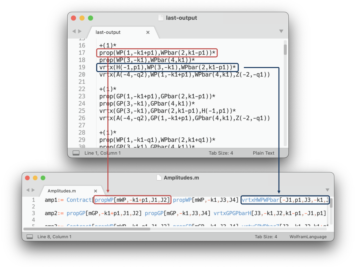
It turns out that the output of Qgraf [Nogueira:1991ex] contains all the information required to write one-loop amplitudes. One just needs to reorganize that information; this task is performed by FeynMaster, as illustrated in fig. 1.1.
Figure 1.1: Conversion of the Qgraf output (top) to a file with the amplitudes for FeynCalc (bottom).
Yet, an automatic conversion from Qgraf to FeynCalc is only really useful if the Feynman rules contributing to the amplitudes (e.g. propWP and vrtxHWPWPbar in the definition of amp1 in fig. 1.1) are also automatically generated. FeynMaster thus resorts to FeynRules [Christensen:2008py, Alloul:2013bka], which yields the complete set of Feynman rules for a given Lagrangian. FeynMaster then writes those rules in a way that FeynCalc can read them, and uses the information of the FeynRules output to automatically generate the model file for Qgraf. In this way, by defining a Lagrangian, one has automatic access to both Feynman rules and amplitudes, all of them defined in the user-friendly setup of FeynCalc.
Another crucial ingredient of FeynMaster is the automatic generation of counterterms. Given that one-loop amplitudes are in general divergent, their study is severely deficient unless one can render them finite. This requires the calculation of the total counterterm for the process under investigation, which in turn requires the determination of the complete set of individual counterterms contributing to it.
FeynMaster not only automatically determines the complete set of counterterms for all the possible processes, but also automatically calculates the total counterterm for the process at stake in a particular subtraction scheme (modified minimal subtraction, ). As a matter of fact, FeynMaster can automatically calculate the total counterterm not only for one process, but also for a sequence of processes. This happens in such a way that, in each process of the sequence, a different individual counterterm of the theory is determined. Thus, by choosing an appropriate sequence, a model can be fully and automatically renormalized with a single FeynMaster run.
All of these steps are rendered more intuitive thanks to the visual interface of FeynMaster. Instead of simply generating the necessary elements for FeynCalc to perform the different calculations, FeynMaster also automatically prints three different types of PDF files. First, it prints the Feynman rules, both for the tree-level interactions and the counterterms; for each rule, the Feynman diagram (drawn with feynmf [Ohl:1995kr]) and the Feynman rule are presented side-by-side.
Second, FeynMaster draws all the Feynman diagrams contributing to the process at stake. Finally, it prints the results of the FeynCalc calculations, which includes not only the amplitudes, but also counterterms. An illutration of these PDF outputs can be seen in fig. 1.2, for scalar QED.
Figure 1.2: Set of PDF outputs automatically generated by FeynMaster in scalar QED: the Feynman rules for the tree-level interactions (left), the Feynman rules for the counterterms (top), the expressions and the counterterms in (right), the Feynman diagrams (bottom).
The files are all written in LaTeX, which allows an immediate inclusion of their content in a paper.
We show in fig. 1.3 the articulation of the different components that constitute FeynMaster as a whole.
Figure 1.3: Articulation of the different components of FeynMaster. All of them are governed by the Python subroutine General, which is not shown. See text for details.
The different colors represent different types of components: in green, the two files that trigger the total run; in blue, the three software that FeynMaster is based on; in gray, intermediate files that chain the whole process; in beige, the main outputs; finally, in red, the subroutines composing FeynMaster. These subroutines are characterized in table 1.1.
Subroutine
Language
Purpose
Addendum
Mathematica
generate the Qgraf model and rules for FeynCalc
Amperate
Python
convert the Qgraf output into amplitudes
ControlExtract
Python
extract information from the Control file
Converter
Python
convert notations
Definitions
Mathematica
make definitions and replacement rules for FeynCalc
Drawing
Python
draw Feynman diagrams
Finals
Mathematica
handle the final expressions of FeynCalc
FRExtract
Python
extract information from the model file
FunctionsFM
Mathematica
provide extra functions for FeynRules and FeynCalc
General
Python
coordinate all the remaining subroutines
IntGauss
Fortran
perform gaussian integrations
JustConvert
Python
support Converter
Preamble
Mathematica
make definitions and lists for FeynRules
Printer
Python
draw and print the Feynman rules
Renapp
Mathematica
generate the counterterms of the model
SupReno
Mathematica
perform renormalization
WriteToPreTeX
Mathematica
generate and print the final expressions
Table 1.1: Subroutines composing FeynMaster 2.
Finally, as already suggested in the Introduction, one of the most striking advantages of FeynMaster is its flexibility. More than just producing the outputs we just mentioned, FeynMaster allows the user to manipulate intermediate and final results, due to the user-friendly features of FeynCalc and Mathematica. This flexible character will be described in more detail in appendices and .
1.2 Comparison with other software
We now provide a brief explanation of how FeynMaster relates to other frameworks which also study particle physics processes at the one-loop level. Among those more closely related to FeynMaster, we select four: GRACE [Belanger:2003sd], FormCalc [Hahn:1998yk], GoSam [Cullen:2011ac, Cullen:2014yla] and NLOCT [Degrande:2014vpa] (for reviews comparing different software, see refs. [Harlander:1998dq, Denner:2019vbn]).
Before entering the comparison, let us consider a preliminary aspect. As we just noted, one of the major advantages of FeynMaster is its flexibility. However, software based on other frameworks (such as FORM [Kuipers:2012rf]) can be much faster than FeynMaster. Actually, if one is interested in obtaining the numerical result for a one-loop process with hundreds of diagrams in a well known model, other software can be preferable. If, however, one wants to use a slightly different model, or ascertain some properties of the analytical results, or make sure to have no problems with interfaces between different software, or simply obtain a printed list of the Feynman rules, then FeynMaster is an interesting alternative. In this sense, the purpose of FeynMaster is not compete with the five aforementioned programs, but rather to enrich the flexibility of FeynCalc by creating a unified platform around it that performs a vast list of tasks.
Let us now consider the referred programs. GRACE is a software that aims at numerically computing cross sections. It generates Feynman rules from a model, generates and draws Feynman diagrams, and writes the differential cross section in a Fortran file. Unlike FeynMaster, it is not restricted to 2 particles in the final state; it employs other software for the numerical integration and event generation; it also addresses renormalization, and calculates counterterms in the on-shell renormalization scheme. However, it cannot calculate one-loop processes that do not exist at tree-level, such as . And although it performs algebraic calculations, it does not seem to allow a large margin for the user to manipulate analytical expressions.
FormCalc is a program that calculates tree-level and one-loop Feynman diagrams based on both FORM and Mathematica. It combines the speed of the former and the vast amount of instructions of the latter. It gets the amplitudes from FeynArts [Hahn:2000kx] and generates an output to numerically evaluate the one-loop integrals with LoopTools. Although FormCalc is excellent for fast results, it lacks the flexibility to perform simple manipulations involving Dirac algebra or Lorentz contractions.
GoSam is designed to an automated calculation of one-loop amplitudes for multi-particle processes. Like FeynMaster, it uses QGRAF to generate the Feynman diagrams in symbolic form, and also uses both Python and feynmf to draw the diagrams. Like GRACE, GoSam produces a Fortran file required to perform the evaluation of one-loop matrix elements. But unlike FeynMaster, it uses helicity amplitudes formalism, and makes renormalization for QCD corrections only. And although it generates one-loop amplitudes, it seems to be mostly focused on numerical evaluation, and not on allowing a manipulation of intermediate or final expressions.
NLOCT determines the UV counterterms for any Lagrangean in an automated way. It requires an interaction with both FeynRules and FeynArts, and works only in the Feynman gauge. It not only obtains the Feynman rules for the counterterms, but also computes the analytical expressions for these counterterms in the on-shell renormalization scheme.
In conclusion, although some of software considered here are more powerful than FeynMaster in some specific tasks (e.g. FormCalc for fast results), FeynMaster exploits the strength of FeynCalc to allow a practical manipulation of the analytical expressions. In addition, FeynMaster condenses in itself a multiplicity of tasks, so that there is no need to convert (and hence there are no obstacles in converting) between different software. All of this renders FeynMaster a truly flexible framework.
Chapter 2 Selection of the true vev
In this chapter, we present an introduction to the selection of the true vev, which is closely related to a discussion on tadpole schemes.
Tadpole schemes have been discussed in recent years in the context of the renormalization of models with extended scalar sectors [Krause:2016oke, Krause:2016xku, Kanemura:2017wtm, Krause:2017mal, Altenkamp:2017ldc, Krause:2018wmo, Dudenas:2018wlr, Denner:2018opp, Krause:2019oar, Dao:2019nxi, Altenkamp:2019wht, Denner:2016etu, Denner:2019xti, Denner:2017vms, Krause:2019qwe] (a recent work [Dudenas:2020ggt] is devoted to this discussion, focusing especially on gauge dependence).
And indeed, they constitute an important aspect in the treatment of any gauge theory with SSB. However, we believe that a clear description of this topic is still missing in the literature. Actually, from our point of view, the language normally used to address tadpole schemes tends to be misleading. We thus found it relevant to clarify this discussion.
We do so in such a way that we do not restrict the discussion to a particular model. The goal, in fact, is to introduce the topic of tadpole schemes in a general gauge theory with SSB. Yet, we shall give special emphasis to the SM, given its universally known character and its preponderance in modern particle physics. In addition, the SM provides an ideal framework for an introduction to the selection of the true vev, since it is simple enough to allow a clear description of the problem, but simultaneously complex enough to reveal several important details.
We extend the discussion to models with two Higgs doublets, as an example of an extended scalar sector.
As shall be seen, the introduction of a second scalar doublet slightly increases the complexity of the problem, since there will be more than one vev. As a consequence, some features not present in the case of the SM will show up, and thus must be conveniently clarified. The discussion can then be easily generalized to a model with a more elaborated scalar sector, since the inclusion of more vevs does not constitute a significative addition of complexity.
The chapter is organized as follows: in section 2.1, we perform a tree-level description of the SM, showing how the true vev is selected in this simple context; then, in section 2.2, we consider the SM up to one-loop level, and clarify several aspects related to the selection of the true vev; finally, in section 2.3, we discuss the case of the 2HDM.
2.1 Standard Model: tree-level
We essentially focus one sector of the SM (the potential, ); we also resort to other sectors, which we cannot introduce in detail.
Reviews of the SM can be found in refs. [Denner:1991kt, Romao:2012pq, Denner:2019vbn]. We closely follow the notation of the latter; this reference ([Romao:2012pq]) introduced several parameters—all dubbed , with different indices—to allow for different sign conventions used in the literature. Throughout this thesis, and unless stated otherwise, we use the sign convention defined by taking all ’s positive.111
Refs. [Denner:1991kt, Denner:2019vbn] choose , and the remaining ’s positive. In general, we follow the conventions of ref. [Romao:2012pq] (although we use and instead of and , respectively).
Note that the paremeter of ref. [Romao:2012pq] is four times smaller than that of refs. [Denner:1991kt, Denner:2019vbn], and the unitary transformations that diagonalize the fermions in ref. [Romao:2012pq] are the dagger of those in refs. [Denner:1991kt, Denner:2019vbn].
Let us then focus on potential of the SM. We write it as:
(2.1)
where and real positive constants, and is the Higgs doublet, which can be parameterized as:222
The parameterization is based on section 3.1.6 of ref. [Denner:2019vbn]. We took to be real, positive and in the lower component of the doublet without loss of generality.
(2.2)
Here, is the Higgs field, while and are the neutral and charged would-be Goldstone fields, respectively. Besides, is a real and positive parameter, which turns out to be non-arbitrary. In fact, perturbation theory
fixes its value.
The reason is that fields used in perturbation theory must represent small excitations around the state of minimum energy of the theory.333
For details, cf. e.g. section 28.1 of ref. [Schwartz:2013pla] or section 4.1.1 of ref. [Bohm:2001yx].
In other words, the state around which the small excitations of fields take place—i.e. the state where they vanish, let us identify it with —must correspond to the state of minimum energy. As a consequence, must be precisely given by the value that ensures that, at the state (i.e. for vanishing fields), the theory has its minimum energy (in short, its minimum).
The state is called the vacuum, and the Green’s functions (GFs) used in perturbation theory correspond to the vacuum expectation value (vev) of a time-ordered products of fields. Generically,
(2.3)
where represents the time-ordering operator; in what follows, we use the short notation instead of , for simplicity.
In this way, all GFs correspond to vevs. However, we usually associate the name ‘vev’ to non-null 1-point functions (i.e. non-null GFs with just one field or, more generally, with just one multiplet). As we now show, the Higgs doublet configures one such vev; and since it is the only multiplet of the theory with this property, we associate the term ‘vev’ to the vacuum expectation value of , .
Going back to : as we saw, to determine its value we must find the minimum of the theory, which in turn is given by the minimum of the potential. Since we are considering a tree-level description, the minimum of the potential can be determined classically, by taking derivatives of the potential in order to the fields. Or, what is even simpler, we can take derivatives in order to the doublet . Then, if we recall that and are both positive, we realize that the minimum of the potential is verified if and only if obeys:
(2.4)
where is defined as:
(2.5)
The quantity is the true vev: it is the value of that corresponds to the minimum of the potential.444
The notion ‘true vev’, as well as equivalent notions such as ‘proper vev’, ‘correct value’, ‘true minimum’, are common in the literature [Fleischer:1980ub, Denner:2019vbn, Denner:1991kt, Krause:2016oke, Peskin:1995ev, Krause:2017mal, Barroso:2012mj, Schwartz:2013pla, Cheng:1985bj].
What we just found is that perturbation theory requires (i.e. the quantity that we introduced in eq. 2.2) to be equal to the true vev , defined in eq. 2.5.
To better illustrate this point, suppose that we did not choose eq. 2.4, but rather .
In that case, the Lagrangian would have a linear term in ,
(2.6)
with defined by
(2.7)
as can be verified by inserting eq. 2.2 in eq. 2.1 and expanding the terms. Since we would be choosing , then would not vanish, which would imply that would have a non-null vev, .
But that would be inconsistent: the fields used in perturbation theory (like ) must vanish when evaluated at , which in turn must describe the state of minimum energy. If , nothing of this holds.
Note that eq. 2.6 corresponds to the Feynman diagram and rule555
In this diagram, the cross means that there is no momentum corresponding to that point.
(2.8)
The presence of such structure always indicates that we are selecting the false vev, i.e. choosing a value for
which does not lead to the state of minimum energy—in which case perturbation theory is not consistent.
We dub both the term on the l.h.s. of eq. 2.7 and the Feynman diagram in eq. 2.8 a tree-level tadpole. The tree-level tadpole always corresponds to the linear term in the scalar field.
And the conclusion is this: if the theory generates a tree-level tadpole, we are not selecting the true vev, i.e. we are not choosing to be equal to . Conversely, if we do make this choice (eq. 2.4), the tree-level tadpole vanishes:
(2.9)
As we want to have a consistent perturbation theory, we select the true vev;
this implies, as predicted, that the vacuum expectation value of is non-vanishing:
(2.10)
The selection of the true vev is straightforward at tree-level, as we just saw. But this will not be the case at higher orders.
To properly introduce that scenario, we consider some aspects that shall prove useful.
We start by noting that, with eq. 2.4, eq. 2.2 becomes:
(2.11)
Then, the masses of the particles become proportional to [Denner:2019vbn]:
(2.12)
Here, , and are the masses of the , and Higgs bosons, respectively; and are the and couplings, respectively;
is the mass of the fermion of type (where , for the down-type quarks, up-type quarks and leptons, respectively), represents the Yukawa matrix for fermions of type and and are the unitary matrices that lead the fermions of type to the mass basis (for details, cf. ref. [Denner:2019vbn]).
We also introduce the weak mixing angle , such that
(2.13)
and
(2.14)
where we used the short notation , , and where is the electric charge.
Besides, we can use the relations in eq. 2.12, as well as
(2.15)
where is the CKM matrix, to replace the original set of independent parameters of the SM,
(2.16)
by the (also independent among themselves, but related to the former) parameters [Denner:1991kt]:
(2.17)
Whichever the set chosen, the independent parameters must be experimentally determined. The set of eq. 2.17 is thus more convenient, since all the parameters contained in it have an intuitive physical meaning (i.e. they can be easily related to experimental quantities) [Denner:1991kt, Bohm:2001yx].
Finally, using eqs. 2.5, 2.12 and 2.14, we can write and as:
(2.18)
If, however, we decided to ignore the fact that , we could use eq. 2.7 (instead of 2.4) to obtain:
(2.19)
which, at this point, is just a more complicated (and rather useless) way of writing eq. 2.18, since . Later on, though, it shall prove useful.
2.2 Standard Model: up to one-loop level
2.2.1 Finite -matrix elements
When we go up to one-loop level, the parameters of the theory no longer have an intuitive physical meaning.
As a matter of fact, they have no meaning at all: they are UV divergent.
In what follows, these parameters are dubbed bare parameters and are identified with the subscript “”.
In non-abelian gauge theories with SSB like the SM, the divergences end up cancelling in physical predictions of -matrix elements
[tHooft:1971akt, tHooft:1971qjg, tHooft:1972tcz, Lee:1972fj, Lee:1974zg, Lee:1973fn, Lee:1973rb], so that the latter become meaningful.
Such cancellation can be carried out through different approaches (cf. e.g. ref. [Denner:1991kt] and references therein); in this thesis, we follow the counterterm approach.
Here, in order to obtain finite -matrix elements, we renormalize the bare parameters.666
An excellent introduction to renormalization can be found in ref. [Schwartz:2013pla].
This involves equating them with the sum of renormalized (i.e. finite) quantities and (infinite) counterterms; taking the Higgs boson mass as an example, we say
(2.20)
where the first term on the r.h.s represents the renormalized parameter, and the second represents the counterterm. Then, the renormalization is completed by fixing the counterterms.777
In this chapter, we do not aim at fixing the counterterms, as we do not intend to renormalize the theory. Several examples of counterterm-fixing can be found in chapter 5, where we renormalize the C2HDM.
Finally, note that the attainment of finite -matrix elements also requires the renormalization of LSZ factors, which we discuss in appendix .
2.2.2 Independent parameters
The Higgs boson mass used in eq. 2.20 belongs to the set of parameters in eq. 2.17. To ensure that all -matrix elements are finite, only one set of bare independent parameters needs to be renormalized;
we can choose either the bare version of eq. 2.16,
Given their physical relevance, we choose the latter.888
Note, however, that the renormalized parameters like will only be physical (i.e. they will only correspond to observables) if on-shell subtraction conditions are used; more details can be found in section 2.2.8 below. This means that the parameters therein contained must be renormalized (in particular, they must be split into renormalized parameter and counterterm, just like in eq. 2.20), while those in eq. 2.21 need not be subject to that process.
Indeed, if we choose the set of parameters in eq. 2.22 as independent, then the parameters in eq. 2.21 are dependent—that is, they can always be written in terms of the independent parameters of eq. 2.22. And since the latter will be renormalized, the ones in eq. 2.21 do not have to be submitted to this process. Yet, although one does not have to renormalize dependent parameters, it may be convenient to do so, as we now clarify.
2.2.3 Renormalizing for convenience
Let us consider the cosine of the weak angle. Given eq. 2.13, and since we are taking eq. 2.17 as the set of independent parameters, it follows that is a dependent parameter.
In the context of the up-to-one-loop theory, eq. 2.13 is written in terms of bare quantities,
(2.23)
Now, as a dependent parameter, does not need to be renormalized. To say it clearly, -matrix elements will not be divergent if we do not renormalize .
In that case, though, we need to replace it everywhere by , and then renormalize and (if we just kept on using , we would run into problems, since is a divergent quantity).
In this method, vanishes from the theory, since it was replaced everywhere.
Consequently, there is no such thing as a renormalized version of eq. 2.23.
But this is one reason why, although it is not necessary, it is convenient to renormalize : one may find it convenient to have eq. 2.23 valid for the renormalized parameters as well (and not only for the bare parameters).
Then, we introduce a new parameter, , such that
(2.24)
where and are the renormalized masses of the and the bosons, respectively.
To see how and are related, we just expand the r.h.s. of eq. 2.23:
(2.25)
So, using eq. 2.24, and neglecting second order terms, we conclude that and are related by:
(2.26)
This allows us to define a counterterm , such that
(2.27)
with
(2.28)
These equations illustrate another motivation for the renormalization of : if we replace it using eq. 2.23 and renormalize and , we end up having more counterterms than if we renormalize (compare eqs. 2.26 and 2.27).
Of course, is given by eq. 2.28, so that we always end up having the same number of counterterms. Nonetheless, the manipulation of expressions can become quite easier if we use the l.h.s. of 2.28 instead of the r.h.s.999
In this simple case, the difference in number of counterterms in not significative, so that this discussion does not seem very relevant. Yet, the difference can be very significative in more complicated cases.
But this reveals another important consequence of the renormalization of , namely: the counterterm is fixed.101010
The renormalization condition 2.28 follows from eqs. 2.27 and 2.24. Had we chosen , with , then we would have freedom to fix the finite parts of (the divergent parts of and must necessarily be equal, as both and are assumed to be finite). In that case, though, by comparing with eq. 2.23, we would necessarily have , with and given by eqs. 2.24 and 2.28, respectively. Hence, the freedom in defining the finite parts of would result in the introduction of yet another variable—the alternative renormalized parameter —, corresponding to a fixed (and in general complicated) expression. The choice adopted in eqs. 2.27, 2.24 and 2.28 is not only simpler, but has the additional advantage that the finite parts of the renormalized parameters are independent of the finite parts of counterterms.
In fact, if we define eqs. 2.27 and 2.24, and given eq. 2.23, we have no freedom to choose : it is (and must be) given by eq. 2.28. This is a simple consequence of the fact that is a dependent variable; and, as a dependent variable, it is fixed—that is, fixed by eq. 2.23. So, the same way is a dependent, fixed variable, so is a dependent, fixed counterterm.
What we just did with the cosine of the weak angle applies to all dependent parameters. That is, a bare dependent parameter does not need to be renormalized, although it can be renormalized for convenience. If one decides not to renormalize it, one must replace it by the corresponding independent parameters, and then renormalize the latter. Alternatively, one can renormalize the bare dependent parameter itself—introducing a renormalized version for it, as well as a counterterm. Yet, just as the bare parameter is dependent and fixed, so will the renormalized parameter and the counterterm be dependent and fixed.
2.2.4 Finite Green’s functions
What we have been describing so far—renormalization of parameters of the theory—is motivated by the need to generate finite -matrix elements, as we noted. If, in addition, we intend to obtain finite GFs (and not simply finite -matrix elements), the logic we apply to the parameters in eq. 2.21 should be extended to fields as well. In that case, fields are also identified as bare fields and are split into renormalized ones through a counterterm; for example,
(2.29)
where is the renormalized Higgs field and the counterterm. Therefore, assuming that we want to get finite GFs, we must renormalize both the parameters and the GFs.
2.2.5 The true vev
What about the vev?
Just like at tree-level, we are interested in selecting the true vev;
and just like at tree-level, the true vev is the one for which the linear terms in the Higgs field vanish. However, since we are considering the theory up to one-loop level, the true vev is no longer the same as it was at tree-level.
That is to say, the true vev is no longer the same as it was in the original, bare theory. In fact, the bare vev—i.e. the vev that is the true vev in the bare theory (the vev which we have been identifying with in section 2.1, but now identify with in the context of the up-to-one-loop theory)—is characterized by the fact that it obeys the bare minimum relation,
(2.30)
But since we are now considering the theory up to one-loop order, we can consider a conceptually different vev: the true vev of the up-to-one-loop theory, which we identify in the following with .
The new quantity corresponds to the true minimum of the effective potential. The effective potential, , includes not only the bare terms (which, as we saw, can be split into renormalized terms and counterterms), but also the one-loop terms.
This suggests that, in order to select the true vev at up-to-one-loop order,
we must ensure the vanishing of linear terms in the Higgs field in the effective potential. It is to this vanishing that we now turn.
The first thing to notice is that we want such vanishing to happen before we renormalize the theory. In other words, we want to select the true vev before we initiate the process which a) expands bare parameters and fields into renormalized ones and counterterms, and b) fixes the different counterterms. Although the two processes—selection of the true vev and renormalization—are close to each other (as shall be discussed in detail), the former is performed before the latter.
We thus consider the bare doublet, .
We follow the same stategy as in tree-level, by parameterizing the doublet with a generic quantity :
(2.31)
From what we have been discussing, the selection of the true vev of the up-to-one-loop theory will happen if and only if . However, as we are about to see, there is more than one consistent way to obtain this equality. These different ways are called tadpole schemes, and we are about to study two of them in great detail. To antecipate a little, one of the tadpole schemes will split in two terms, while the other scheme will equate it immediatly with in a single term. In both schemes, we will have , i.e. the true up-to-one-loop vev will be selected. Yet, to account for the different approaches, we keep the generic parameter for now.
Whichever the method used to select the true vev, the linear terms in the Higgs field in the effective potential must vanish.
If we insert into the bare version of the potential,
we obtain only part of the effective potential: we still lack the one-loop quantities. This can be easily solved by defining coefficients for the one-loop terms. Since we are interested in the linear terms in the Higgs field only, we just have to be concerned with the coefficient of that term, which we identify with .
Then, we find that the totality of linear terms in the Higgs field in the effective potential, , are such that:
(2.32)
Hence, the linear terms in the Higgs field vanish if and only if we have:
(2.33)
This is the key condition for the selection of the up-to-one-loop true vev:
if the quantity introduced in eq. 2.31 obeys eq. 2.33, then it corresponds to the true up-to-one-loop true vev .
As we suggested, eq. 2.33 can be verified by manipulating in different ways, the so-called tadpole schemes.
We now proceed to characterize separately the two tadpole schemes we alluded to; we will explain in detail how the selection of the true vev is interconnected with the renormalization of the theory.
Before that, however, three final notes.
First, since the r.h.s. of eq. 2.33 is of one-loop order, so will the l.h.s. also be. This means that, when we renormalize the theory—and thus split the bare field according to eq. 2.29—, the contributions of the counterterm to eq. 2.32 can be neglected; antecipating that, we can replace the bare field in eq. 2.32 by the renormalized one, .
In that case, is the one-loop linear term in . That is, is the one-loop tadpole,111111
Throughout this thesis, the hatched circle represents by default a one-loop non-renormalized generic GF.
(2.34)
Second, as we have been suggesting, the selection of the true vev is a procedure which is prior to the procedure of renormalization.
In particular, counterterms (which result from the identification of bare parameters or fields with renormalized ones and counterterms) only show up after the true vev has been selected. Nonetheless, and as we shall see, it can be useful to think of the l.h.s. of eq. 2.33as a counterterm, the so-called tadpole counterterm ,
(2.35)
Then, the first term on the r.h.s. of eq. 2.32 is simply , and is represented as:
which in turn can be diagrammatically represented as:
(2.38)
On the other hand, as we will discuss in detail in section 2.2.10, the name counterterm for can be misleading, precisely because is not a regular counterterm (we insist, the selection of the true vev is prior to renormalization).
However, since will contribute to the counterterms of other GFs, we keep the name.
Finally, both tadpole schemes will obey eq. 2.33, which means that, in of both of them, eq. 2.32 is zero. And this in turn implies that, in both of them, there are no linear terms in .
But there is an important detail here. What we have been saying is that linear terms in will always cancel out; and by ‘linear terms’ we mean terms which are linear only in (i.e. 1-point functions in , just as ).
But this does not mean that a term like cannot exist. In fact, all we ensure with eq. 2.33 is that 1-point functions in vanish; but since is not a 1-point function in , there is nothing preventing it from appearing—even if it is proportional to .
In other words, our goal never was that by itself is zero, or that it vanishes from the theory, but rather that it vanishes from the Higgs 1-point function (because we wanted the Higgs 1-point function to vanish).
We realized that this required eq. 2.33 to be true, which ensures that the only two quantities that contribute to the Higgs 1-point function and precisely cancel.
But suppose that, in another GF, contributes, but in such a way that there is no added to it.
That is to say, in that GF we do not have something like:
(2.39)
but rather like:
(2.40)
In that GF, then, will not cancel: it will contribute to the GF. On the other hand, eq. 2.33 is always valid, as it is the assurance that we have selected the true vev. Hence, eq. 2.40 becomes:
(2.41)
This means that, in that GF, there will be a one-loop tadpole. Only, there is nothing wrong with this, since this does not spoil 2.33, i.e. it does not spoil the fact that there are no 1-point functions in . Actually, both tadpole schemes will see one-loop tadpoles appearing in GFs (other than 1-point functions).
We should not let terminology confuse us: if by tadpole we mean a term linear only in (a 1-point function in ), then both schemes will have no tadpoles; if by tadpole we mean a one-loop tadpole contributing to GFs other than 1-point functions, then tadpoles will emerge in both schemes. In order to avoid misunderstandings, we shall name proper tadpoles to the former (i.e. to 1-point functions in ) and broad tadpoles to the latter (i.e. to one-loop tadpoles contributing to GFs other than 1-point functions).
We now introduce the two schemes, following ref. [Denner:2019vbn] closely.
2.2.6 Fleischer-Jegerlehner tadpole scheme
It is in this scheme, introduced by Fleischer and Jegerlehner in 1981 [Fleischer:1980ub], that is split into two terms,
(2.42)
where means that the equality is valid in the Fleischer-Jegerlehner tadpole scheme (FJTS). Recall that is the bare vev, so that it obeys eq. 2.30—an equation which we will use repeatedly, and which can in particular be used to derive the relations
(2.43)
which is just the bare version of eq. 2.18. Moreover, in this scheme, the bare masses are defined in terms of the bare vev:
(2.44)
In its turn, in eq. 2.42 will be responsible for cancelling the one-loop proper tadpole, . To see how this comes up, we can insert the bare Higgs doublet (eq. 2.31) in the bare potential using eq. 2.42, and consider only the terms which are linear in . We find:
(2.45)
The fact that will cancel the one-loop tadpole implies that it is formally of one-loop order, so that we can neglect . Moreover, since should cancel the one-loop term linear only in , the term responsible for such cancellation should also be linear only in . That is, using the definition 2.37, should be multiplying the linear term in in eq. 2.45, which leads to the identification:
(2.46)
This is consistent with eq. 2.35; to see it explicitly,
(2.47)
where we neglected . Using now eq. 2.44 to solve for in eq. 2.46 in the one-loop approximation fixes it to:
(2.48)
Now, to begin to ascertain the impact of these equations on the renormalization of the theory, note that, because is of one-loop order, we can replace all the bare parameters and fields in eq. 2.45 for their renormalized equivalents.
As for , we use eq. 2.44 to replace it by and then we replace these parameters for their renormalized versions.
Therefore, using eqs. 2.44 and 2.48, we can rewrite eq. 2.45 as:
(2.49)
This equation represents the totality of terms in the effective potential that, in the FJTS, are proportional to .
The first term on the r.h.s. will precisely cancel the one-loop proper tadpole (i.e. the one-loop 1-point function) of , just as eq. 2.37 predicts. So, in the end of the day, there will be no proper tadpoles in the theory, as intended.
However, we see in eq. 2.49 that broad tadpoles will be around. For example, the term will contribute to the Higgs 2-point function; and the (which is a one-loop tadpole, recall eq. 2.37) contained in it is an example of what we called a broad tapole. Indeed, it is a one-loop tadpole contributing to a GF other than a 1-point function (in this case, the 2-point function of the Higgs boson).
The reason why it may be useful to think of as a counterterm is that we can include the new term in the set of counterterms of the Higgs 2-point function. Such set then becomes:121212
The factor in the last term (instead of ) is due to the .
(2.50)
It turns out that eq. 2.48 allows an interesting reorganization of the counterterms.
Let us start by noting that the cubic Higgs coupling is given by
(2.51)
and the zero-momentum Higgs propagator by
(2.52)
Then, combining these equations with eq. 2.36, we find131313
We draw small black circles on the dashed lines to highlight the presence of a tree-level propagator.
In order to realize the importance of these results, note that the most general structure of a renormalized (connected) 2-point GF at one-loop level is given by:
(2.55)
This is a universal relation (valid for every tadpole scheme), where the straight lines represents any type of particle.
The terms on the r.h.s represent respectively the (non-renormalized) one-particle irreducible (1PI) one-loop GF, the corresponding counterterm, the reducible diagram with a one-loop tadpole, and the corresponding counterterm.
Now, due to eq. 2.37 (diagrammatically represented in eq. 2.38), the last two terms of the r.h.s. of eq. 2.55 necessarily cancel. We just found this explicitly for the Higgs 2-point function in eqs. 2.53 and 2.54. As a consequence, the complete 2-point function at one-loop includes only the first two terms of the r.h.s. of eq. 2.55, that is, the 1PI terms: the non-renormalized one-loop function and its counterterm, respectively.
Moreover, the counterterm (i.e. the second term on the r.h.s. of eq. 2.55) in general includes a broad tadpole, as we saw in eq. 2.50 for the Higgs 2-point function. Hence, we can split it explicitly in two parts:
(2.56)
In the Higgs 2-point function, however, we found a curious result:
the -part (given by the last term in eq. 2.50) precisely cancels eq. 2.53.
This means that, instead of letting the last two terms on the r.h.s. of eq. 2.55 cancel (so that the complete 2-point function at one-loop includes only the first two terms of that side), we can let the broad tadpole contained in the second term cancel against the fourth term, in which case the complete 2-point function at one-loop is given by the first term, the third term and the second without the broad tadpole. That is, in the FJTS, instead of
(2.57)
we can write
(2.58)
The two equations are equivalent. In particular, both include a broad tadpole: in eq. 2.57, it corresponds to the second term on the r.h.s., while in 2.58 it corresponds to the third term on the r.h.s.
But why would we want to use eq. 2.58 instead of 2.57? It turns out that, with software such as FeynMaster, it is much easier to calculate a reducible Feynman diagram with a one-loop tadpole than to derive a term like the last one in eq. 2.50.
In fact, by using eq. 2.58, we do not have to go through all the process involved in obtaining the last term in eq. 2.50—which involves separating into and as in eq. 2.42, identifying with the quotient in eq. 2.48 and looking in eq. 2.49 for terms contributing to the GF we are after. Instead, we can just use Feynman rules to calculate the reducible diagram with a one-loop tadpole.
Actually, this applies to all the other GFs as well: not only to 2-point functions for particles other than the Higgs, but also to GFs with more than 2 particles. That this is true can be easily proven if we realize that, inserting eqs. 2.29, 2.42 and 2.48 inside eq. 2.31,
then and always appear together. Therefore, for every term in the Lagrangian with , there is a term with instead. So, for every -point function with a contribution, there is a -point function with a Higgs field instead of the ; and with that Higgs field, we can always form a reducible diagram (with a one-loop tadpole) which, using eqs. 2.34, 2.37 and 2.52, precisely equals the -point function with a broad tadpole. For example, for the 2-point function (in the FJTS), we have:
(2.59)
and
(2.60)
In the same way, for the Higgs 3-point function (in the FJTS), we have:
(2.61)
where we showed only the term with the broad tadpole, and
(2.62)
In sum: in the FJTS, we can account for all the broad tadpoles—the new terms generated through contributing to GFs other than the 1-point function—by including all possible reducible diagrams with one-loop tadpoles in all possible GFs. Note that it is easy to predict which GF will contain broad tadpoles: considering eqs. 2.42 and 2.48 again, we see that there will be a term with for every term with . It follows that broad tadpoles show up for every GF whose tree-level contribution contains a , which includes all the 2-point functions and some 3-point functions.
2.2.7 Parameter-renormalized tadpole scheme
We now consider the other scheme, introduced in ref. [Denner:1991kt] and dubbed parameter-renormalized tadpole scheme (PRTS) in ref. [Denner:2018opp].
Here, is not separated in two, but is immediately taken as the true vev :
(2.63)
Besides, there is no mention of in the PRTS. In particular, the bare masses are defined in terms of :
(2.64)
To obtain the bare Higgs mass, we isolate the quadratic terms in in the bare potential; we find:
(2.65)
Finally, we can combine eqs. 2.35 and 2.63 to obtain:
(2.66)
Like before, proper tadpoles vanish: eq. 2.38 is valid. Yet, just like before, broad tadpoles (again, one-loop tadpoles like contributing to GFs other than 1-point functions) will be around after renormalization. To see it explicitly, note that we can use eqs. 2.65 and 2.66, as well as the first relation of eq. 2.64, to conclude that shows up inside and only:
(2.67)
Then, it is easy to show that the totality of terms proportional to in the effective Lagrangian is:
(2.68)
Hence, while the first term on the r.h.s. cancels the one-loop 1-point function of the Higgs boson, all the other terms represent broad tadpoles: the second and third terms contribute to the 2-point function of the charged and neutral would-be Goldstone bosons, respectively, the fourth term to the 3-point function containing one Higgs and two charged would-be Goldstones, and so on.
Some final notes should be considered.
First, in the PRTS, eq. 2.66 can be seen as the relation that defines . Or, as we could also state it, the true vev is defined as the value which obeys eq. 2.66, since it is this relation that ensures that the theory is free from proper tadpoles.
Second, equation 2.68 implies that, in the PRTS, appears only inside terms of the potential; what is more, it does not contribute to the 2-point function of any physical particle.141414
It is easy to see that both these statements hold in the PRTS for a general scalar sector. Concerning the circumstance that 2-point functions of physical particles never contain broad tadpoles, this is a consequence of the definition of the bare mass of the physical particles. The bare mass, indeed, is defined as the collection of terms that contribute to the bilinear term of the field at stake; so, even if broad tadpoles are included in those terms (and in general they are), they are subsumed under the definition of the bare mass, and thus do not show up contributing to the 2-point function.
That broad tadpoles show up exclusively in the potential (i.e. contribute exclusively to GFs coming from the potential) will be shown below.
In other words, although broad tadpoles are in general present in the PRTS, they are only present in a very specific set, namely: the GFs that come from the potential and that do not correspond to a 2-point function of a physical particle.151515
And, of course, that do not correspond to 1-point functions, by definition of broad tadpole.
So, for example, there are broad tadpoles in the Higgs 3-point function, but none in the Higgs 2-point function; and there are broad tadpoles in the 2-point function of would-be Goldstone bosons, but none in the 2-point functions of gauge bosons or fermions. All in all, then, in the PRTS there are no broad tadpoles contributing to any 2-point functions of physical particles (which will be relevant when we discuss renormalization in the on-shell subtraction scheme).
Third, one cannot in general calculate broad tadpoles in the PRTS through reducible diagrams with one-loop tadpoles, like in the FJTS, since there is no equivalent to eq. 2.48 in the PRTS.161616
This does not mean that broad tadpoles in the PRTS can never be calculated through reducible diagrams with one-loop tadpoles. In some particular cases, that may be possible. In the SM, such scenario happens in the 2-point functions of non-physical scalars. A simple explanation is that, in these cases, the broad tadpole contribution in the PRTS is precisely equal to that in the FJTS: compare eqs. 2.49 and 2.68. In any event, eq. 2.55 continues to be valid in the PRTS, and the last two terms of its r.h.s. still cancel. As a consequence, it is mandatory to write the terms in the potential in terms of and track down all the terms in which it shows up.
This task can be simplified by realizing that, at tree-level, eq. 2.7 allows to antecipate eq. 2.66: one just needs to promote the tree-level true vev and the tree-level tadpole to the up-to-one-loop vev and , respectively.
In fact, the terms which will have in the up-to-one-loop theory are precisely those with a tree-level tadpole in the tree-level theory, and only those.171717
This allows to explain why, in the PRTS, broad tadpoles show up exclusively in the potential (recall note 14).
Indeed, the equations for the tree-level tadpoles (the minimization equations) exclusively involve parameters of the potential.
And this is the advantage of writing eq. 2.19 instead of 2.18 at tree-level: it allows to anticipate eq. 2.67 in the PRTS.
Finally, note that eq. 2.67 implies eq. 2.66. This means that the relations in eq. 2.67 are sufficient to ensure that no proper tadpoles will be around. Therefore, the strategy outlined in the previous paragraph—rewriting the tree-level relations in terms of the tree-level tadpole and then, when considering the up-to-one-loop theory, promoting the to —is sufficient to ensure that the true vev is chosen.
2.2.8 Comparison between the two tadpole schemes
2.2.8.1 Fundamental differences
There are two fundamental differences between the two tadpoles schemes we presented. The first one has to do with the wayis verified—and not with the value of . In reality, as we saw, both schemes end up having ; this implies that there are proper tadpoles in neither of them, although this comes at the price of having broad tadpoles in both. But although both obey , they do it in different ways: the PRTS takes that relation from scratch; the FJTS, by contrast, picks . Naturally, this difference has consequences, which we now describe in detail for the two schemes.
In the PRTS, the true vev is used. This is no longer fixed by the tree-level relation 2.5, but rather by eq. 2.66.
As a consequence, not every tree-level relation can be immediately taken as a bare relation. In other words, when passing from the tree-level to the up-to-one-loop level, it is not always true that, for a certain tree-level relation, one can simply convert all the parameters involved to their bare versions, assuming that the relation written in terms of bare parameters will also hold. This is because tree-level relations which assumed the vanishing of the tree-level tadpole must be rewritten without this assumption (as we did in eq. 2.19). Then, the relation will be valid for bare parameters if and only if the tree-level tadpole is identified with the tadpole counterterm (see eq. 2.67).
It turns out that broad tadpoles show up in GFs of the potential only, and never in 2-point functions of physical particles. Yet, they must be calculated by explicitly tracing down .
The FJTS is clearly different. By splitting into ,
it introduces broad tadpoles in every Feynman rule which has a in the bare theory—in particular, in 2-point functions of physical particles. On the other hand, broad tadpoles can be accounted for by considering one-loop tadpole insertions in all possible GFs. Furthermore, since the FJTS uses (the bare vev, obeying eq. 2.30), the tree-level relations can be immediately taken as bare relations, and there is no need to be careful with tree-level tadpoles; we saw an explicit example of this in equations 2.18 and 2.43.
On top of all this, there is a second fundamental difference between the two schemes, which is the way bare parameters are defined. In the PRTS, they are defined in terms of through eqs. 2.64 and 2.65, whereas in the FJTS they are defined in terms of through eq. 2.44. This difference leads to an interesting discussion concerning gauge dependence,
which we now introduce.
2.2.8.2 Gauge dependence
Let us consider a generic parameter , renormalized according to:
(2.69)
and let us assume that depends on the vev. We are interested in ascertaining the gauge dependence of the variables involved in this equation: not only in the context of both tadpole schemes (PRTS and FJTS), but also in the context of two common subtraction schemes: the on-shell subtraction (OSS) scheme and the modified minimal subtraction () scheme.181818
Subtraction schemes are different prescriptions to define the finite part of a certain counterterm. For more details, see section .
In the PRTS, the vev which depends on is . But if we consider eq. 2.66, we see that is related not only to the parameters and , but also to ; and while the former are gauge independent by construction, the latter is defined by a one-loop process through eq. 2.37, which turns out to be gauge dependent [Degrassi:1992ff]. It follows that , by depending on , will also be gauge dependent. Now, in OSS, the parameters are renormalized in such a way that they (i.e. the renormalized parameters) correspond to observables---which implies that they are gauge independent.191919
Care should be taken with cases of ‘indirect’ OSS renormalization. For example, the renormalization of mixing angles can be determined through symmetry relations (cf. appendix ). In this case, the parameter counterterms are fixed by field counterterms, which in turn may happen to be fixed through OSS. In this ‘indirect’ (since parameter counterterms are not directly fixed via OSS, but rather through OSS-fixed field counterterms) OSS renormalization, the renormalized parameters will in general not correspond to observables, and hence will in general be gauge dependent.
In that case, is gauge independent, and compensates the gauge dependence of [Denner:2016etu].
In fact, if represents a generic gauge parameter, it follows from eq. 2.69 that:
(2.70)
so that, in OSS,
(2.71a)
(2.71b)
(2.71c)
In , however (and still in the context of the PRTS), there is nothing forcing the renormalized parameter to be gauge independent. Therefore, both and will in general be gauge dependent.
The situation changes if we consider the FJTS. Here, the vev which depends on is . This vev, in contrast to , is a bare quantity and, as such, gauge independent. Consequently, is also gauge independent. We now prove that this implies that the three quantities present in eq. 2.69 are gauge independent in both OSS and .
That this is true in OSS follows immediately from eqs. 2.70, 2.71a and
(2.72)
Note, by the way, that for everything to be consistent, the GFs in the FJTS must include the broad tadpoles. This applies, in particular, to 2-point functions (recall eq.
2.58)—which is crucial to ensure the gauge independence of parameter counterterms in OSS. Indeed, parameter counterterms (like mass counterterms) in OSS are defined in terms of 2-point functions evaluated in the on-shell (OS) limit; but these are in general gauge independent if and only if the reducible diagrams with one-loop tadpole are included in them [Degrassi:1992ff]; that is,
(2.73)
(where means that the OS limit is considered), in such a way that
(2.74)
This means that, if we did not include the reducible diagrams with the one-loop tadpole, we would end up with a gauge dependent 2-point function, and hence a gauge dependent parameter counterterm—which is precisely what happens in the PRTS (recall that, in the PRTS, there are no broad tadpoles contributing to the 2-point functions of physical particles).
Going back to the FJTS, we now turn to . Here, the counterterm is defined as
proportional to , which contains a divergence (see section for details).
On the other hand, is finite (by definition of renormalized parameter), so that it is independent of . Hence,202020
We have been assuming that depends on the vev; as we saw, this implies that, in the PRTS, is gauge dependent. If, however, does not depend on the vev, eq. 2.75 also holds in the PRTS.
(2.75)
In conclusion, renormalized parameters and their counterterms are gauge independent in the FJTS: both in OSS and .
The PRTS, by contrast, is plagued by gauge dependences: only the renormalized parameter is gauge independent, and only if it is renormalized through OSS.212121
Recall that, as mentioned in note 19, counterterms fixed in the FJTS via an ‘indirect’ OSS renormalization will in general be gauge dependent.
As it is clear, the parameter counterterms will in general contribute to -matrix elements, so that one should in principle ensure that both are gauge independent, in order to obtain gauge independent -matrix elements (nonetheless, see discussion in section ). In the PRTS, we just saw that, using OSS, the parameter counterterms are in general gauge dependent.
However, if all parameters are renormalized using a momentum-subtraction scheme (like OSS), the gauge dependence ends up cancelling in renormalized functions (and hence in physical predictions). In fact, a momentum-dependent subtraction scheme is such that the counterterms are defined as a function of a one-loop integral evaluated at a specific momentum (we ignore terms of derivatives, which are irrelevant for the argument). Accordingly, a renormalized GF corresponds to the non-renormalized function evaluated at a general momentum, minus the same non-renormalized function evaluated at a specific momentum. Now, the gauge dependence of the non-renormalized function is related to that of the reducible diagrams with the one-loop tadpole (recall eq. 2.74). But since those diagrams do not depend on the momentum, we conclude that the gauge dependence cancels in the renormalized GF [Denner:2016etu]. I thank Ansgar Denner for clarifications on this aspect.
2.2.8.3 Observable differences
Are there physical (i.e. observable) differences between tadpole schemes?
In a first approach, one might think that, in this respect, tadpole schemes are like subtraction schemes.
As is well known, although observables in a renormalized theory must be independent of subtraction schemes, such independence must only be verified if one had an exact (i.e. including all-orders in perturbation theory) calculation. More precisely, if one would perform an exact calculation in two different schemes, the relations between observables in the two cases would be equivalent.
Yet, calculations performed at a certain finite order in perturbation theory (i.e. including only a certain number of loops) will in general depend on the subtraction scheme.222222
The differences between calculation performed in two different schemes, though, are of higher order[Bohm:2001yx].
The question now is whether the same happens in calculations with different tadpole schemes. The answer is no: differences in calculation at a certain finite order between consistent tadpole schemes cancel exactly. That is, one does not need to get the exact result to obtain equivalent descriptions between two tadpole schemes: finite order calculations are also equivalent. As matter of fact, we are about to see that the relevant connected Green functions are the same.232323
It follows that, in the FJTS, when one considers processes that do not come from terms in the potential, the broad tadpoles showing up in the renormalized connected one-loop amplitude must cancel between themselves. The reason is that, on the one hand, and as we just saw, there cannot be differences at finite orders in connected GFs calculated in different tadpole schemes; on the other hand, there are no broad tadpoles in the PRTS outside of the potential.
2.2.9 The need to select the true vev
In the previous sections, we have been concerned with selecting the true vev of the up-to-one-loop theory. We introduced two different ways to achieve such selection, and we compared them in detail.
What we should now realize is that we really did not need to perform such selection. To say it clearly, we did not need to choose the true vev of the up-to-one-loop theory [Collins:1984xc, Appelquist:1973ms, Bohm:2001yx, Denner:2016etu].242424
I am particularly indebted to Ansgar Denner for several clarifications on this topic.
This is in contrast to what happened at tree-level. As we saw in section 2.1, indeed, the selection of the true vev at tree-level was a necessary condition for perturbation theory to be consistent. To recap, fields used in perturbation theory should correspond to small excitations around the (true) minimum of theory. So, if we were to choose a vev which would not ensure this basic condition, perturbation theory would not make sense; the poles of the propagators would in general not have corresponded to the physical masses, so that -matrix elements could not be calculated.
Conversely, if the correct (or true) vev is selected, in such a way that the minimum of the potential is chosen, then perturbation theory is sound, i.e. well-defined.
The point we should now stress is this: as long as perturbation theory is well-defined at tree-level (i.e. at lowest order), it will stay well-defined at higher orders.
The reason is simply that higher orders correspond to small corrections (i.e. small perturbations) relative to the lowest order; consequently, if
the fields were correctly defined at the lowest order, then perturbation theory is not spoiled at higher orders. This holds, in particular, for the vev. In fact, the true vev of the up-to-one-loop theory differs from the true vev of the tree-level theory by higher orders, as it is obvious. So, the consistency of perturbation theory is not spoiled if we choose a vev that differs from the true vev by higher orders. In other words, precisely because higher order are small, perturbation theory is consistent both when we select the true tree-level level, and when we choose vevs that differ from it by higher order effects.
But this seems to lead to a problem. Indeed, suppose that, when we consider the theory up-to-one-loop level, we use the bare vev. In that case, the one-loop proper tadpole (i.e. one-loop 1-point function of the Higgs boson) will not vanish. It turns out that the one-loop proper tadpole is a divergent GF. Hence, our theory will have a divergence, which is not removed.
Yet, that is really not a problem. Divergences in the theory constitute a problem when they lead to divergent predictions. This is because the theory should describe the physical (i.e. observable) reality, which is obviously free from divergences. So, if the theory makes predictions which are divergent, then it is deeply sick. But the point is that 1-point functions do not correspond to any prediction; they are not like 2-point functions (which are intrinsically related to a physical—i.e. observable—mass), nor like 3-point functions (which are intrinsically related to a physical—i.e. observable—coupling). In 1-point functions, there is really nothing physical, i.e. observable. Therefore, the fact that they are divergent does not imply that the theory will end up making divergent observable predictions.
As we have been suggesting, physical meaning is obtained from GFs with more than one external leg. However, connected GFs with more than one external leg do not depend on the selection of the vev. This was explicitly proven in ref. [Denner:2016etu]; in what follows, we reproduce their proof.
We consider two different generating functionals for the SM: , defined in terms of the field , and , defined in terms of the field , in such a way that the two fields are related by:
(2.76)
with an arbitrary constant. Then, and ignoring the remaining fields of the theory,252525
We omit the dependence of both the current () and the fields ( and ) on the space-time coordinate ().
(2.77a)
(2.77b)
Note that we wrote in , because the theory is the same as the one described by , and due to eq. 2.76. Now, since the path integral measure is invariant under a constant shift, we can use eq. 2.76 to rewrite eq. 2.77b as:
(2.78)
Therefore, the generating functionals of the connected GFs and are related via:
(2.79)
As a consequence, the connected GFs of the two descriptions are related by:
for n=1,
(2.80a)
for .
(2.80b)
In the end, then, the connected GFs with more than one external leg () do not depend on the arbitrary constant .
For this reason, even if two descriptions of the same theory decide to expand their field around different vevs (so that the fields differ by a constant), the connected GF with more than one external leg will be the same.262626
It should be clear that this also holds at tree-level; the only requirement is that the propagator is defined with the correct mass.
To understand this aspect, suppose the theory, , for a real scalar field, and for and real positive parameters. With this choice of parameters, there is no SSB, so that the field configuration that leads to the minimum happens for the constant solution .
Now, in the most obvious description, perturbation theory is performed with the field itself, which describes small excitations around the vacuum . The mass of the propagator is . However, one can also define (for an arbitrary constant ) and describe the perturbation theory using . In this case, all the terms containing should be considered as vertices (even the 1-point functions and the 2-point functions), which means that the mass of the propagator of is still . Then, if the symmetry factors are taken care of, and if different powers of are treated as formally independent (so that a proper expansion in orders of is performed), one can verify that the dependences on vanish in all connected GF with more than one external leg. Note that, in both descriptions (the one using and the one using ), the propagator has the same mass , which must always be determined from the true minimum of the theory; that is to say, the mass of a propagator must always correspond to the coefficient of the bilinear terms of the field that describes small excitations around the true minimum (in this sense, it is mandatory to select the true vev at tree-level). As long as this is the case, perturbation theory can be consistently defined by fields that differ from each other by a constant, as we just saw. I thank Ansgar Denner for clarifications on this point.
In sum, when condering the theory up to one-loop level, we really do not need to select the true vev to that order. This means that eq. 2.37---which is a necessary condition to ensure that the true vev of the up-to-one-loop theory is selected---is really not necessary to have a consistent description of the theory.272727
Contrary to what is sometimes mentioned in the literature [Gambino:1999ai, Dudenas:2020ggt], eq. 2.37 is not needed for a correct definition of the Legendre transformation that yields the generating functional of the 1PI GFs.
It is relevant to ascertain what happens if eq. 2.37 does not hold (i.e. if the true vev of the up-to-one-loop theory is not chosen). Suppose that, in the theory considered up to one-loop level, we select the bare vev. In that case, there will be no tadpole counterterm whatsoever; in fact, if we choose in eq. 2.35, then , due to eq. 2.30. Accordingly, we see from eq. 2.55 that the complete 2-point function becomes:
(2.81)
But this is precisely what we found for the FJTS, eq. 2.58. Actually, this is hardly a surprise. To see it in detail: in the FJTS, the field we used was defined by reference to the up-to-one-loop true vev, which we wrote as ; in eq. 2.81, by contrast, the field was defined by reference to the tree-level true vev . So, the fields in the two description differ by a constant .
But as we just saw in eq. 2.80b, if we define two fields that differ by a constant, the complete connected 2-point function does not depend on that constant. Hence, and since the constant is directly proportional to the tadpole counterterm (eq. 2.48), we conclude that, in the FJTS, the complete connected 2-point function does not depend on the tadpole counterterm. Or, which is the same, the terms in the complete 2-point function that depend on must cancel:
(2.82)
A similar relation holds also for 3-point functions. In conclusion, the FJTS (where the true vev at up-to-one-loop level was selected due to the introduction of the quantity ) is equivalent to a scheme where the bare vev is selected. Note that, in this case (i.e. if the bare vev is chosen), one still finds the advantages of the FJTS which result from the use of that vev in the bare relations—namely, the fact that tree-level relations can be immediatly converted into bare relations, as well as the advantages concerning gauge independence.
Despite of this, one can argue that, when considering the theory up-to-one-loop level, it is convenient to select the true up-to-one-loop vev. The advantage would be that, with that choice, eq. 2.38 holds, which implies that the last two terms of the r.h.s. of eq. 2.55 cancel, which in turn implies that one does not have to consider reducible diagrams with one-loop tadpole insertions (third term of the r.h.s. of eq. 2.55).
However, as we discussed at the end of section 2.2.6, we believe that there is no inconvenience in such reducible diagrams. As a matter of fact, we find it highly preferable to let the terms with tadpole counterterms cancel (as in eqs. 2.58 and 2.81).
2.2.10 Renormalization
2.2.10.1 Renormalized tadpoles?
Let us go back to the case where we select the true vev, as we have been discussing in the previous sections. This is by far the most common approach in the literature, and usually goes by the name of
tadpole renormalization [Krause:2016oke, Krause:2017mal, Altenkamp:2017ldc, Denner:2017vms, Krause:2018wmo, Dudenas:2018wlr, Denner:2018opp, Krause:2019oar, Dao:2019nxi, Altenkamp:2019wht, Denner:2016etu, Denner:2019xti, Denner:2019vbn, Dudenas:2020ggt].
Some authors [Altenkamp:2019wht] even define and (corresponding to the bare and the renormalized tadpole, respectively), such that:
(2.83)
Then, in the FJTS, is taken to be:
(2.84)
which is zero due to eq. 2.30. Then, using eqs. 2.37 and 2.83,
(2.85)
By contrast, in the PRTS, is taken to be:
(2.86)
which is not zero, but rather equal to , through eq. 2.66. Using eq. 2.83, it then follows that:
(2.87)
2.2.10.2 A misleading name
Although this interpretation—according to which tadpoles were renormalized—is sometimes presented, we find it highly misleading, for two main reasons.
First, renormalization is a process through which unphysical divergences are removed from the theory. In the previous sections, however, our focus was never divergences, but only tadpoles. Our goal was never to remove the divergences of tadpoles, but rather to remove tadpoles altogether. Even in section 2.2.9, where we realized that it is not imperative to select the true up-to-one-loop vev (and hence to remove proper tapoles), the discussion was centered on the selection of the vev; indeed, the main question was ‘which vev to select?’, and not ‘how to remove divergences?’.
Second, a very simple argument against the thesis according to which we renormalized something is the fact that the quantities that we are left with after the ‘renormalization’ are not finite at all. Indeed, in an attempt to be consistent with the idea of tadpole renormalization, eq. 2.83 is introduced. This equation just looks like a regular renormalization equation, similar to eqs. 2.20 and 2.27, with a non-renormalized term (), a renormalized one () and a counterterm (). But this equation is misleading in both tadpole schemes: in the FJTS, and as we just saw in eq. 2.85, the ‘renormalized’ parameter is equal to , which is the one-loop proper tadpole and therefore a divergent quantity. In the PRTS, the parameter we are left with is not even the renormalized one, but rather the quantity given in eq. 2.86, which is also divergent.
The same applies, by the way, to the vevs: as we are about to discuss in detail, both and are divergent.282828
Moreover, the parameter introduced in the FJTS in eq. 2.42 is no counterterm; rather, it is a parameter that eliminates one-loop proper tadpoles. Contrary to counterterms, indeed, it allows to renormalize nothing: neither the tadpole (recall eq. 2.85), nor the vev. As a matter of fact, the quantities , and are all divergent.
Therefore, by talking about renormalization, one can be mislead and conclude that the remaining parameters really are renormalized, i.e. finite.
One can argue that eq. 2.33 (or, equivalently, eq. 2.37) is just a renormalization condition for the tadpole, and that other renormalization conditions would be possible, according to what we discussed in section 2.2.9. But this section (2.2.9), by clearly demonstrating that one does not have to get rid of divergences of 1-point functions, shows that the discussion of which vev to select
is not a question of renormalization. That is to say, eq. 2.33 is not a renormalization condition among others, but a selection of vev among others.
All this should convince us that we should not use the term ‘renormalization’ for the subject underlying the different tadpole schemes. In our point of view, the correct description is selection of the true vev. Or, if the true vev is not selected (as suggested in section 2.2.9), the description would be simply selection of the vev.
Unfortunately for the sake of clarity, we were led to identify the l.h.s. of eq. 2.33 with a counterterm, since terms with broad tadpoles can be included in the counterterms of GFs, as in eqs. 2.59 and 2.61. In any event, we find counterproductive the introduction of eq. 2.83, and we believe that the notion ‘tadpole counterterm’ should be used with caution.
Finally, this also means that, unless one actually uses the relations of the theory to choose the vev as an independent parameter, it makes no sense to include the vev—or the tadpole, for that matter—in the list of independent parameters of the theory, as if it needed to be renormalized. As we saw in section 2.2.2, only independent parameters need to be renormalized; and the vev is not chosen as independent parameter in the usual approaches to the SM (in particular, it is not independent neither in eq. 2.21 nor in eq. 2.22).
2.2.10.3 Actual renormalization
The present discussion becomes more interesting when we realize that, after the selection of the true vev, one does speak of renormalization. Indeed, as we just saw, after we eliminated proper tadpoles through the choice of the true vev, the parameters we are left with are divergent. Actually, not only the broad tadpoles are divergent (they correspond to one-loop GFs), but the vev used to define the bare masses as well. This is not surprising, since these are precisely bare masses, so that there is no reason why the vevs involved in their definition— in the FJTS and in the PRTS---should be finite.292929
The fact that is the true vev of the theory might lead us to think that it has some physical meaning, in which case the vev used to define the masses in the PRTS would need to be finite. But this is incorrect: has no physical meaning, i.e. there is no observable associated to .
These vevs have no physical meaning whatsoever: not only can they be gauge dependent (as in the PRTS is), but they can also be divergent—and both in the FJTS and in the PRTS are, in fact, divergent. In the following, we call the vev used to define the masses the bare-mass-defining-vev, or bmd-vev for short. In the FJTS, then, the bmd-vev is , while in the PRTS it is .
Now, as we suggested, unless one uses the relations of the theory to replace one of the independent parameters in eq. 2.22 by the bmd-vev, the latter will be a dependent variable. In that case, then, the bmd-vev is just like the cosine of the weak angle discussed in section 2.2.3: on the one hand, it is fixed (in this case, by the mass relations); on the other hand, it does not need to be renormalized.
If one decides not to renormalize it, one must replace it everywhere by the parameters it depends on, and the latter must be renormalized, just as we saw for . However, and as we also saw in that case, it may be convenient to renormalize the bmd-vev.303030
In the literature, what usually happens is that the bmd-vev is not renormalized, whereas the sine and cosine of the weak angle are renormalized for convenience [Denner:1991kt, Denner:2019vbn]. What this means is that, while the bmd-vev is replaced by the quantities it depends on and the latter are renormalized (so that the bmd-vev does not show up anymore in the theory), the bare parameters and are replaced by renormalized parameters and counterterms, and these renormalized parameters and counterterms in general contribute to the Feynman rules.
To see this in detail, we consider again separately the different tadpole schemes.
We start with the FJTS. Based on eq. 2.44, we can write:
(2.88)
Note that and belong to eq. 2.22, so that they must be renormalized, while must not (although we renormalize it for convenience, as we did with in section 2.2.3). To proceed to the renormalization of these parameters, we define the counterterms , and such that:
(2.89)
At this point, if we want to have an equivalent to eq. 2.88 for renormalized quantities, we must introduce the parameter :
(2.90)
Just like in the case of the cosine of the weak mixing angle, we can relate and by expanding the r.h.s. of eq. 2.88. Then, if we define a counterterm obeying the relation
(2.91)
we conclude that:
(2.92)
Some aspects should not be neglected here. First, contrary to what usually happens (e.g. in eq. 2.89), we cannot define the renormalized quantity in eq. 2.91 without index—since the parameter is already attributed to the true vev; we thus defined . Second, this parameter is indeed renormalized and thus finite. Third, the counterterm is fixed and exactly equal to the totality of counterterms that showed up at the expansion of eq. 2.88. Finally, it is only when we renormalize the bmd-vev that we can employ the relation eq. 2.90 (it is a matter of course that one can always assume that eq. 2.90 is valid and not mention explicitly any counterterm ; in doing so, however, eqs. 2.91 and 2.92 are implicitly used).
In the PRTS, the situation is different. Here, the bmd-vev is , not ; we can use eq. 2.64 to write
(2.93)
Then, proceeding in a similar way as before, we now introduce the relation
(2.94)
which ends up leading to:
(2.95)
By comparing eqs. 2.92 and 2.95, we realize the importance of using the superscripts FJ or PR: the two equations are different (since the counterterms involved are calculated in different ways in the different tadpole schemes), although they would look the same without the superscripts.
2.2.10.4 An alternative approach
We have been describing a general approach to the treatment of the theory when considered up to one-loop level, according to which one is faced with two different tasks (in the following order): first, one chooses which vev to select (and, possibly, through which way or scheme to perform that selection); then, one takes care of renormalizing the theory.
An alternative approach is also possible. It aims ab initio at a single goal: removing all divergences of the 1PI GFs. In that case, all one is really concerned about are divergent parts (finite parts can be addressed in a later moment).
Just as in our approach, an essential question is: how should one treat the vev?
In the alternative approach we are now discussing, one usually considers a counterterm for the vev, as if the vev was a normal parameter. Then, three questions become relevant:
1.
Is such counterterm really necessary (in order for all divergences of the 1PI GFs to be removed)?
2.
If so, what value should it have?
3.
How is such counterterm related to other counterterms?
In simple models, such as the linear sigma model, one finds that a counterterm for the vev is necessary, although it is the same as the counterterm for the scalar field [Peskin:1995ev, Bohm:2001yx]. Consequently, the counterterms available in the theory before SSB are enough to remove all divergences (cf. also ref. [Srednicki:2007qs]).
In more complex theories, such as the SM, the situation is more subtle, due to gauge-fixing terms. A vev counterterm is also necessary, but it will only be equal to the counterterm for the scalar field in some specific gauges [Chankowski:1991md, Sperling:2013eva, Grimus:2018rte, Dudenas:2020ggt]; in general, one needs a vev counterterm that is independent of the counterterm for the scalar field.
Although such an alternative approach is legitimate, we find it less transparent, and we will not consider it in the following.
2.3 2HDM
So far, we have been exploring properties of tadpole schemes in the SM, where there is just a single Higgs doublet. New features appear when one considers additional doublets. We discuss the simplest case, that of two Higgs doublets. We start with the case where CP is assumed to be conserved in the potential, and then address the case with general CP violation.
Although the former configures a description which, as we shall argue in chapter 3, is not theoretically sound, the discussion of vev selection (and tadpole schemes) in that case is nonetheless relevant, for two reasons: first, it has been repeatedly considered in recent literature [Krause:2016oke, Krause:2016xku, Kanemura:2017wtm, Krause:2017mal, Altenkamp:2017ldc, Krause:2018wmo, Dudenas:2018wlr, Denner:2018opp, Krause:2019oar, Dao:2019nxi, Altenkamp:2019wht, Denner:2016etu, Denner:2019xti, Denner:2017vms, Krause:2019qwe]; second, a model with two Higgs doublets and CP conservation, by itself, is not unsound;313131
The problem with the real 2HDM, as shall be seen, is that it enforces CP conservation in a part of the theory, while allowing CP violation in another.
hence, the discussion of the selection of the vev in that case is not only legitimate, but also instructive.
We do not provide an exhaustive treatment neither in the CP-conserving case nor in the CP-violating; rather, we illustrate only the relevant new features concerning tadpole schemes.
2.3.1 CP conservation
We begin with the tree-level description.
Supposing two Higgs doublets and , we have:
(2.96)
with and real vevs.
It is usual to define the variable such that:
(2.97)
as well as the total vev , such that:
(2.98)
with:
(2.99)
Let us now consider what happens when we consider the theory up to one-loop level. The case with two scalar doublets is a simple generalization of that with just one scalar doublet. In the SM, when considering the theory up-to-one-loop level, we discussed how to select the true vev, so that all proper tadpoles would vanish from the theory. With two scalar doublets, there are two vevs, but the principle is the same. Specifically, one may select the true vevs—identified in the following (in the context of the theory considered up to one-loop level) with and —, which again guarantees that no proper tadpoles show up.
2.3.1.1 FJTS
The FJTS for a general Higgs sector was studied in detail in ref. [Denner:2016etu]. Here, we present but a brief sketch of its application to a theory with two scalar doublets. As a trivial extension of what we found with one doublet, the bare doublets and are written in terms of and , respectively. Each one is split into two terms:
(2.100)
where and correspond to the bare vevs (the vevs that were the true vevs in the bare theory) and and to the quantities that will cancel the one-loop tadpole terms. Similarly to what we had in eq. 2.44, the bare masses of the particles of the theory are defined in terms of the bare total vev,
(2.101)
an expression that directly follows from eq. 2.98.
Concerning and , one needs to rotate them into the mass basis (i.e. the basis where the scalar fields are well-defined) in order for them to cancel the one-loop tadpole terms of the physical scalar fields.
By defining the CP-even physical scalar fields with the usual notation and (with mass and , respectively),
one can accordingly define the rotated versions of and
as and . Then, one can prove the relations:323232
For details, cf. section .
(2.102)
where and are the one-loop tadpoles of and , respectively.
Following the same line of thought as in the SM, one concludes that all the broad tadpoles in the FJTS can be consistently accounted for by including all the possible reducible diagrams with one-loop tadpoles in all possible GFs.333333
In theories with two scalar doublets, the variable usually represents not only a relation between the two vevs, but also a mixing angle that establishes the connection between two different bases of fields (cf. eq. 3.3.1 below). Now, it is sometimes read in the literature [Krause:2017mal] that, when using the FJTS, one has to be careful to distinguish between the two meanings of . The point is that, if a certain term involves in the sense of a relation between the two vevs, then such term follows from the expansion of the scalar doublets; in that case, the splitting in eq. 2.100 will generate—besides the term at stake—also terms with or . The same will not happen for terms involving in the sense of a mixing angle. As a consequence—so the argument goes—, one must be careful to distinguish the two scenarios. However, as already noted, all the terms with or —that is, all the terms with broad tadpoles—can be accounted for by including all the possible reducible diagrams with one-loop tadpoles in all possible GFs. In this case, there is no need to distinguish the two different meanings of .
The generalization of the FJTS from one scalar doublet to two is thus quite simple.
The use of in the context of the FJTS is also straightforward. As we saw, in the FJTS the bare relations can be immediately derived from the tree-level ones, since the bare vevs are used in the definitions. Then, the bare version of eq. 2.97 in the FJTS is:343434
A couple of points should be stressed here. First, note that the definition of is not modified by and . Recall that these variables were only introduced in the scalar doublets in order to cancel the one-loop tadpoles, as we saw in detail in the case of the SM. In that case, it would make no sense to change the definition of to include such quantities. Actually, if we did so, we would be absorbing some of the broad tadpoles in the definition of —which would render a consistent use of the FJTS very complicated. Indeed, one would not be able to include in all possible GFs all the reducible diagrams with one-loop tadpoles, as some of them would be absorbed inside . It follows that, in the FJTS, even if and are each split into two terms, the definition of is still given by eq. 2.103.
Second, it should be clear that using and is simply an alternative to using and . And just as in the SM, in the FJTS, the renormalization of (discussed in section 2.2.10.3) has nothing to do with and the elimination of proper tadpoles (discussed in section 2.2.6), the same happens with two scalar doublets in the FJTS: the renormalization of and is independent of and the elimination of proper tadpoles. Therefore, since and are just an alternative to and , the same conclusion follows for them, namely: in the FJTS, the renormalization of and is independent of and the elimination of proper tadpoles.
(2.103)
When renormalizing theories with two scalar doublets, the variable is usually taken as an independent parameter, whereas , and are not. As such, must be renormalized, according to:
(2.104)
whereas , and must not. And while one could always renormalize these variables for convenience (as we did with above), there is no real advantage in doing so. Thus, immediately before renormalization, one should use the dependence relations of the theory to replace those variables for independent parameters. Specifically, one should use eq. 2.88, which also allows one to write
(2.105)
and then renormalize , , and as usual.353535
Alternatively, should one had decided to renormalize and for convenience, one could define and , such that
(2.106)so that the renormalized would obey the relation . Then, together with the definitions:
(2.107)this would lead to the relations:
(2.108)
2.3.1.2 PRTS
In the PRTS with two scalar doublets, the procedure is similar to that of the SM: for one thing, the quantities and are immediately taken as the true vevs; besides, the bare relations that depend on the vevs are written in terms of the true vevs. This means that, just as the SM tree-level relation for the mass of the -boson was , but in such a way that the PRTS bare version of this relation was (with the true vev , not with the bare vev ), in the same way the tree-level obeys eq. 2.97, but the PRTS bare version of this relation is:
(2.109)
Assuming—as in the FJTS—that is chosen as an independent parameter, and , and as dependent ones, one can use eq. 2.93 to write:
(2.110)
and then renormalize , , and as usual.363636
We follow here an equivalent derivation to the one in note 35, but now for the PRTS.
Should one had decided to renormalize and for convenience, one could define and , such that
(2.111)so that the renormalized would obey the relation . Then, together with the definitions:
(2.112)this would lead to the relations:
(2.113)
Finally, recall that, in the PRTS, one cannot in general account for all the broad tadpoles (which, in the PRTS, only show up for terms in the potential) by considering reducible diagrams with one-loop tadpoles. As described at the end of section 2.2.7, one can get a consistent theory by rewriting the tree-level relations assuming that tadpoles do not vanish, and then, when considering the theory up to one-loop level, identify the bare tadpoles with their corresponding tadpole counterterms. Only, while in the SM only two tree-level relations needed to be modified in order to account for all the broad tadpoles (recall eqs. 2.19 and 2.67), in a model with two Higgs doublets there will be more (cf. e.g. eqs. 2.19 of ref. [Altenkamp:2017ldc]).
2.3.2 CP violation
The existence of CP violation leads to generally complex vevs (or, which is equivalent, phases besides the real vevs), which constitute the main novelty when compared to the scenarios studied above. We discuss in detail the FJTS in section .
Here, we restrict ourselves to a very brief comment on the role of phases of the vevs in the PRTS.
Similarly to what we did before, when we consider the theory up to one-loop level, we write the expectation values of the two bare doublets as:
(2.114)
where the quantities , , and are real. As usual in the PRTS, these quantities are identified with the true quantities (without bars):
(2.115)
Hence, just as in the CP-conserving case one had true vevs ( and ), in the CP-violating one also has true phases ( and ). And, just as in the previous models, the values of these true quantities (which are in general divergent) are fixed such that there are no proper tadpoles. This can be ensured in the usual way: rewriting the tree-level relations in terms of bare tadpoles and, when considering the theory in the context of one-loop level, replacing the bare tadpoles by the corresponding counterterms (just as was done above in the SM in eqs. 2.19 and 2.67).
The values of , , and in those relations thus correspond to the true values.373737
The true phases and will in general be non-null. However, one can always use the rephasing freedom of the theory to absorb the (true) values of and in the remaining parameters of the theory.
2.4 Summary
We discussed the selection of the true vev in models with SSB, focusing especially on the SM.
Whereas this selection is trivial when the theory is taken at tree-level, it becomes more involved when one goes up to one-loop level.
On the other hand, although such selection is necessary in the first case,
it is not so in the second. In fact, as we showed, one can find a consistent description of the theory using connected GFs, even if divergent one-loop 1-point functions are not removed.
Nevertheless, we focused on the selection of the true vev of the up-to-one-loop theory.
We described in detail two different ways to implement such selection: the tadpole schemes FJTS and PRTS. We have seen that, by assuring that the theory is free from one-loop 1-point functions (identified as proper tadpoles), both schemes end up introducing one-loop tadpoles contributing to other GFs (identified as broad tadpoles).
After comparing the two schemes, it becomes patent that the FJTS has significant advantages over the PRTS, notably: the triviality to convert tree-level relations to bare relations, the easiness to account for all the broad tadpoles of the theory, and the simplicity to obtain gauge independent parameters and counterterms.
We found that the FJTS is actually equivalent to an approach where the bare vev is used. Thus, and given the comodity with which, using tools such as FeynMaster, reducible diagrams with one-loop tadpoles are calculated, one can simply ignore the selection of the true vev, and use the bare vev throughout.383838
Recall that we are treating theories only up to one-loop level. The elimination of proper tadpoles at higher orders may be preferable.
We argued that, whichever the vev chosen in the context of the up-to-one-loop theory, such selection is not a question of renormalization, but rather an undertaking that precedes renormalization. As we noted, despite the potential convenience in identifying a certain quantity with a tadpole counterterm,
the identification of the selection of the vev with ‘tadpole renormalization’ is misleading, among other reasons because neither vevs nor tadpoles become finite (i.e. renormalized) due to the selection of the true vev. We explained that, when one performs the renormalization of the theory (after the true vev has been selected), the vevs can be treated as regular parameters. As such, they must be renormalized should they be taken as independent, and they can be renormalized for convenience otherwise.
Finally, we discussed the case of models with two Higgs doublets. We have seen that the selection of the true vev in the SM can be easily extended to that case. We analyzed how the parameter (related to the two vevs) should be considered in both the FJTS and the PRTS. We also commented on the case with CP violation, where one also has true phases besides true vevs.
Chapter 3 Is there a real 2HDM?
In this chapter, we address the claim raised in the Introduction according to which the so-called real 2HDM is a theoretically unsound model. In section 3.1, we start by discussing the inconsistency of requiring CP conservation in the potential of the real 2HDM, while allowing for CP violation elsewhere. We argue that, at sufficient high order in perturbation theory, there will be divergences in CP-violating 1-point and 2-point functions that cannot be removed by the counterterms provided by the theory.
We show in section 3.2 that this is precisely what happens in a toy model suffering from the same problem as the real 2HDM. Then, in section 3.3, we investigate the consistency of the real 2HDM itself. There, we present the result for the leading pole of the three-loop 1-point function of the alleged CP-odd physical field of the real 2HDM, together with the details of the calculation.
3.1 Shortcomings of the real 2HDM
Let us consider a gauge theory with
two Higgs-doublets and ,
with the same hypercharge ,
and with real vevs and , such that:
(3.1)
The most general 2HDM scalar potential may be written as
(3.2)
The coefficients
, , and
are real, while
, , and
may be complex.
When extending this model to the fermion sector, one finds
flavour changing neutral scalar interactions, which are very
strongly constrained by experiments on neutral meson systems.
This problem can be solved by imposing a symmetry:
;
[Glashow:1976nt, Paschos:1976ay].
If the symmetry is exact, both the quadratic term
and the quartic terms and vanish.
This has the consequence that the model has no decoupling limit;
that is, one cannot smoothly approach the SM limit by rendering the masses of the new
particles (i.e. the particles resultant from the presence of the second scalar doublet) arbitrarily large.
Such a decoupling is a desirable feature,
especially since the couplings probed by current
LHC data are consistent with the SM predictions,
within errors of order 20% [Khachatryan:2016vau].
Decoupling is recovered by reintroducing
[Gunion:2002zf],
which,
because it breaks softly the symmetry,
does not affect the renormalizability of the theory.111
Cf. e.g. ref. [Cheng:1985bj] page 187 ff. and references therein.
Most articles addressing this model then decide
that both the vevs and , as well as the parameters and , are all real, arguing that CP conservation in the scalar sector has been imposed (choice 1).
One would then proceed to discuss the various implementations of the
symmetry in the fermion sector, and perform a variety of
fits to experiment.
Among these, one must fit the well measured CP violation with origin
in the Cabibbo-Kobayashi-Maskawa (CKM) matrix
[Cabibbo:1963yz, Kobayashi:1973fv],
accommodated by the complex Yukawa couplings (choice 2).
Choice 1 and choice 2 are both assumed by the so-called real 2HDM.
Only, they are incompatible.
In fact, either the CP symmetry is applied to the whole Lagrangian,
in which case the Yukawa couplings are real (which means that one cannot account for the observed CP violation); or, else, the CP symmetry is not applied anywhere, in which case not only the Yukawa couplings are in general complex, but is also in general complex.222
We mention only (and not ) simply because, in the basis of and where and are real, the minimization equations lead to a relation between the phase of and the phase of , so that the latter can be seen as dependent from the former. For details, see section 4.1.1 below.
A compromising scenario—allowing complex Yukawa matrices but excluding —leads to a non-renormalizable theory.
At sufficiently high loop level, indeed, the CP violation
in the quark sector will leak into the scalar sector,
through a divergent contribution that cannot be absorbed by
a counterterm—which was excluded from the theory from the start.
So why do all articles fitting the real 2HDM “model” to experiment
ignore this problem?
Because the divergent contribution can only be shown to happen
in at least
three loops.
However,
precisely because they are divergent, the problem cannot be ignored
if one wishes to use a theoretically sound model.
Given the fact that
the problem seems to occur due to (the lack of)
,
one could be tempted to assume that such a dimension two operator
could not affect renormalizability.
And indeed, it cannot affect renormalizability due to the circumstance that it softly-breaks the symmetry.
But the problem with CP symmetry being
invoked is not
that it is broken by (real or complex); rather,
it is (hardly) broken
by the dimension four Yukawa couplings.
It is true that one can look at the real 2HDM as a limiting case of
the 2HDM, softly broken by a complex .
This model is known as the complex 2HDM (C2HDM), and will be considered in detail in the following chapters.
In that case, one can choose any tree-level values for the parameters,
and, in particular, set
at tree-level.
In that context,
setting at tree-level
does not constitute a problem,
since the theory does have its counterterm and is renormalizable (cf. chapter 5).
Is this the same as the real 2HDM? No, it is not:
setting in the C2HDM means that
we are studying a specific corner of tree-level parameter space
of a more general model. The real 2HDM, where there is no
nor its counterterm, is not a consistent model.
There is a more physical way to state the non-renormalization problem.
In any 2HDM, there are three physical neutral scalars.
In the real 2HDM, the (proclaimed) lack of CP violation in the scalar sector leads to the separation of the three neutral scalars into
one single CP-odd state () and two CP-even states (usually denoted by for the lightest and for the heaviest).
If the CKM CP violation seeps into the scalar sector,
there should be divergent contributions to the - and -
2-point functions, as well as to the 1-point function.
Since such terms are absent from the real scalar sector at tree-level,
there are no counterterms to absorb those infinities,
and the theory is formally inconsistent.
At this point, a hasty reader could argue that Pilaftsis put forward a model [Pilaftsis:1998pe] where he (allegedly) shows to no such problem exists. In Pilaftsis’s model, CP-conservation at tree-level in the scalar potential leads him to define the CP-odd state and the CP-even states and ; yet, CP violation coming from another sector of the theory seeps into the scalar sector at one-loop, thus rendering the - and - 2-point functions and the 1-point function divergent; however, the theory “fortunately” happens to generate counterterms for those GFs [Pilaftsis:1998pe], so that the theory is consistent.
The problem with this argument is that the model by Pilaftsis has a small, but crucial difference regarding the real 2HDM, namely: in Pilaftsis’s model, the fact that all parameters of the potential are real
is a consequence of a basis choice.
In the real 2HDM, by contrast, there is no basis where the generally complex quantities , , and can all be rendered real.
We discuss Pilaftsis’s model in detail in appendix , where we show that it is a sound model.
In the following sections, we argue that the real 2HDM is theoretically unsound.
3.2 A theoretically unsound toy model
We start by considering a toy model, which suffers from the same inconsistency as the real 2HDM. In both models, CP conservation is enforced in a particular sector of an otherwise CP-violating theory.
As a consequence, CP-violating radiative effects end up contaminating
the alleged CP-conserving sector, thus leading to divergences
that cannot be absorbed by the counterterms.
The major feature of our toy model is that such divergences show up
immediately at one-loop order.
Therefore, it constitutes a simple materialization of the
same theoretical pathology that we claim to be present
at three-loop or above in the real 2HDM.
The present model is inspired in the model by Pilaftsis which we alluded to, and which we discuss in detail in appendix .333
Only (we insist), whereas the model discussed in appendix is sound and consistent, the model we discuss in this section is as unsound and inconsistent as the real 2HDM.
Consider two Abelian gauge symmetries and ,
with gauge bosons and ,
respectively.
Suppose also four complex scalars, ,
, and , with charges
(3.3)
(3.4)
where and represent the conserved charges of and ,
respectively.
A discrete symmetry is imposed on the fields, under which:
(3.5)
However, is allowed to be softly broken.
The complete renormalizable Lagrangian can then be written in four terms,
(3.6)
where represents the kinetic
terms444
We assume no - kinetic mixing. and
(3.7a)
(3.7b)
(3.7c)
The parameters , , and are
in general complex, while the remaining ones are real by
construction. The terms involving and
break the symmetry softly.
It is easy to show that the conditions for CP conservation are:
(3.8a)
(3.8b)
(3.8c)
Mimicking the usual real 2HDM treatment,
we take and real
and parameterize
(3.9)
where
, are real and non-negative,
and
, , , and are real fields.
The vevs and break spontaneously the gauge symmetry .
Recall that , , , are in general complex.
But suppose we force CP to be conserved in
by the ad-hoc imposition that
and are real.
This we do in the following. As we will show, though, it will lead to irremovable divergences at one-loop.
We start by determining the minimization (or tadpole) equations.
These are:555
The tadpole equations for and are trivially zero.
(3.10a)
(3.10b)
where represent the tree-level
tadpoles for , , respectively, and
means that the expectation
values of all fields on the r.h.s. of
eqs. (3.9) are set to zero.
Recall that we are taking and as
real parameters. For that reason, the mass matrices for and
, on the one hand, and for and , on the other,
can be separately diagonalized. We thus define the
angles and such that:
where and are the CP-even states, and
and are the CP-odd states, where
is the massless would-be Goldstone boson.666
is eaten by the longitudinal component of in the
unitary gauge through the Higgs mechanism.
The fact that is massless forces to
obey the relation .
As for the sector, the mass matrix is given by
(3.12)
with
(3.13)
where and are real, while is in principle complex.
However, we can rephase through
so that it absorbs the phase of .
In the new basis, then, is real, which implies that
the mass matrix in eq. (3.12) is
symmetric.777
If it were hermitian, one would
need a unitary matrix to diagonalize it, instead of
an orthogonal one. Moreover, note that
real forces the relation
.
We thus need an orthogonal matrix with a new angle
to diagonalize the states:
(3.14)
where and are the (complex)
diagonalized states with (real) masses and .
The model was easily implemented on FeynMaster, which allowed to determine the Feynman rules, counterterms and one-loop results.
When considering the theory up to one-loop level,
the quantities of the original theory are identified as bare quantities. We decide to select the true vev of the up-to-one-loop theory through the PRTS. Recalling the discussion of sections 2.2.7 and 2.3.1.2, it follows from the set of eqs. 3.10 that:
(3.15a)
(3.15b)
where and are the true vevs, and where the tadpole counterterms and are such that
and
, with and
being the one-loop tadpole for and , respectively.
Note that, since we imposed CP conservation in
, there are no tadpole counterterms
for the CP-odd fields.
Specifically, in the mass basis,
(3.16)
But it is easy to see that this is inconsistent in the PRTS.
Indeed, there is a one-loop tadpole for ,
whose diagrams are represented in fig. 3.1.
The sum of diagrams is divergent.
In fact,
(3.17)
in dimensions,
where represents the one-loop tadpole for
and means that we consider
only the terms proportional to inverse powers of .888
Note that, in the paper [Fontes:2021znm], the alternative convention is used. We changed the results to the convention , because this convention is the one that is used throughout the thesis.
Figure 3.1: Feynman diagrams contributing to
the one-loop tadpole of the CP-odd state.
The origin of the problem lies in the fact that we
imposed and to be real.
To clarify this point, let us provisionally
take these parameters to be complex, as they originally were.
By rewriting eq. (3.7a) in terms of bare quantities,
and separating the real and imaginary parts of
and ,
the terms proportional to these parameters are:
(3.18)
As a consequence, when we set
,
we are not including in the model the terms of the
last line of eq. (3.18).
Naturally, since such terms are not in the model,
there is no counterterm for the parameters involved therein.
That is, there is neither
nor .999
The situation
would not be different if we decided
to exclude any other term from the theory. For example,
had we decided not to include the term
proportional to in the model,
there would be no counterterm .
Now, it is a matter of course that this would not be a problem
if the fact that we did not include the terms in the last
line of eq. (3.18) would follow from a symmetry that forbade them.
In other words, should there be a symmetry in the theory that
proscribed those terms, they could logically not be included;
and since the symmetry would prevent any GFs
generated by such terms from showing up, there would never be
divergences involved therein, so that the absence of
counterterms for them would never be a problem.
So, for example, if CP was a symmetry of the theory,
it would preclude those terms, in which case the absence
of and
would not be inconsistent.
However, CP is not a symmetry of theory:
even if we try to impose it in the sector,
it still is violated in the
sector through the phases of and ,
as eqs. 3.8a and 3.8b show.
So, there is no CP symmetry forbidding the terms in
the last line of eq. 3.18.
As a consequence, even if we exclude them, CP-violating radiative effects
can nonetheless contribute to the GFs involved therein.
Such GFs will in general be divergent;
but since the last line of eq. 3.18
were not included in the theory, there will in general
not be enough counterterms to absorb them.
We have already seen one example of GF
whose divergences cannot be removed: the one-loop 1-point
function . Other examples are the one-loop
CP-violating 2-point functions ,
, and
for the scalar-pseudoscalar mixing of ,
, and , respectively.
Their Feynman diagrams are represented in fig. 3.2.
Figure 3.2: Feynman diagrams contributing to the
one-loop CP-violating 2-point functions.
There simply is no
counterterm for these functions, which nonetheless
are divergent. Their divergent parts are:
(3.19a)
(3.19b)
In conclusion, the fact that we imposed
and
to be real leads to several
divergences that cannot be removed from the theory.
There are two ways to heal this model: either CP is
imposed as a whole, or it is not imposed at all.
In the first case, all the three relations in
eqs. 3.8 should be verified, which implies
that there is a basis where , ,
and are all real. In this scenario, therefore,
CP-violating GFs are precluded, which implies,
in particular, that no divergent CP-violating GFs will appear at any order.
This is consistent with what we obtained in
eqs. 3.17 and 3.19,
which vanish in the limit of real and .
In the second case, , , and
are in general complex parameters, which implies
that their counterterms are also in general complex.
Since CP is violated, there are no scalar states with
well-defined CP, and GFs will in general
be CP-violating.
The model is renormalizable as long as all the terms
compatible with the symmetries are included.
Finally, note that, in such a CP-violating scenario,
there may be regions of the parameter space in which
and are real, and and complex.
But this is a completely different situation from that where one
builds a theory taking ab initio and
real, while and in general complex.
In fact, while the former situation corresponds to a
particular solution of a consistent, renormalizable theory,
the latter suffers from the inconsistencies we have shown.
3.3 Probing the real 2HDM
The previous section ought to convince us that the real 2HDM, by imposing CP conservation in the potential sector but allowing it elsewhere, will suffer from the same inconsistencies as the toy model we just presented.
Our goal now is to investigate this inconsistency in the real 2HDM itself. We start by presenting the potential sector of the model, followed by a short analysis of the CP violation originating from the CKM matrix. Then, in section 3.3.3, we perform a three-loop calculation, whose details are given in section 3.3.4.
3.3.1 The potential sector
As suggested in section 3.1, the scalar potential of the real 2HDM reads:
(3.20)
with all parameters real. The doublets can be parameterized as
(3.21)
with real constants, real fields, and and complex fields. The vevs and obey eq. 2.97, i.e. .
In that case, if one inserts eq. 3.21 inside eq. 3.20 and expands the terms, one finds that, since and are real, there are no linear terms for the fields, just as there are no bilinear terms mixing fields with fields.
Accordingly, the fields are identified as CP-odd, and the fields as CP-even.
The requirement that the linear terms in the fields vanish leads to two minimization (or tadpole) conditions; since there were no linear terms in the fields to start with, there are no such conditions for these fields. In what follows, we use the short notation ,
for a generic angle .
The Higgs basis [Lavoura:1994fv, Botella:1994cs]
can be defined by introducing the orthogonal matrix , such that:
The doublets in the Higgs basis are written as
(3.31)
with complex fields, and real fields, and is a real parameter defined as in eq. 2.98, i.e. .
Expanding the terms of the potential, one finds that are already mass states (i.e. they are already diagonalized): and correspond to the charged and neutral would-be Goldstone bosons, respectively, corresponds to a charged scalar boson and to the CP-odd physical state. The states and can be diagonalized introducing the angle , such that:
(3.32)
where and are the CP-even mass states.
3.3.2 CP violation from the CKM matrix
In the real 2HDM, just as in the SM, CP violation arises from the complex
Yukawa couplings.
When the quark fields are rotated into their mass basis,
all CP violation phases are contained in the
CKM matrix [Cabibbo:1963yz, Kobayashi:1973fv].
However, each quark field can still be rephased at will,
thus moving the CP-violating phase around the various entries
of the CKM matrix.
The only rephasing invariant quantity is
[Jarlskog:1985ht, Jarlskog:1985cw, Dunietz:1985uy]
(3.33)
where and (we use the notation of ref. [Branco:1999fs], where Greek letters refer to up-type quarks ,
while Roman letters
refer to down-type quarks ).
There are nine distinct four quark combinations with different flavours:
three combinations for the down-type quarks—, —times three for the up-type quarks—, , and .
Using the unitarity of the CKM matrix,
the following symmetries hold
(3.34)
showing that indeed there is only one independent CP-violating quantity.
The antisymmetry with respect to interchange of same quark-type indices
is easiest to see in the form
(3.35)
where
is the Jarlskog invariant
[Jarlskog:1985ht, Jarlskog:1985cw, Dunietz:1985uy],
defined for example as .
As emphasized by Khriplovich and Pospelov [Pospelov:1991zt]
and by Booth [Booth:1993af]
in the context of the electric dipole moments (EDM)
of the and the electron, the antisymmetry
of is very powerful.
In fact, any CP-violating amplitude from a fermion box diagram will appear as the product
with some amplitude
(3.36)
It turns out that, when all contributions are summed over (, , , and ),
all terms in ,
symmetric under
or will not contribute.
A much more involved analysis along these lines
was used in refs. [Pospelov:1991zt, Booth:1993af]
to show that the SM electroweak contributions to the
EDMs
of the and the electron vanish in the two-loop
and three-loop approximation, respectively.
3.3.3 Three-loop tadpole for in the real 2HDM
We now ascertain whether quark-induced CP-violating effects contaminate the
otherwise CP-conserving scalar sector of the real 2HDM via radiative corrections. Since the quantity that represents quark-induced CP violation in a convention-independent way is the Jarlskog invariant , we are looking for radiative corrections to the 2HDM which contain this quantity.
As the simplest check, we have looked for diagrams proportional to contributing to the tadpole.101010
Strictly speaking, and as we saw in section 2.2.9, even if a 1-point function ends up being divergent, that does not necessarily imply that the theory is inconsistent. On the other hand, just as in the toy model discussed in section 3.2, the inconsistency of the real 2HDM should manifest itself in divergences contained both in 1-point and 2-point CP-violating GFs. Hence, if we find divergent CP-violating effects in 1-point functions, that is a clear indication that the 2-point functions will be sick, with disastrous consequences for the real 2HDM.
This can only happen in amplitudes with a) at least four vertices containing each a factor of and b) a vertex to couple to .
Consequently, the first possible appearance of in
-tadpoles is at three loops.
An example of a pair of diagrams yielding the
Jarlskog invariant is shown in fig. 3.3.
Figure 3.3: Example of pair of Feynman diagrams where factorizes (for fixed ). They differ only by the direction of fermion flow.
It goes without saying that the complexity of a calculation at three-loop level—even the most simple one, like the tadpole of —cannot be compared to the complexity of the one-loop calculations of section 3.2.
For a start, the complete calculation of three-loop tadpole of would require the renormalization of this process up to that order; unfortunately, such enterprise is not available in the literature and is beyond the scope of this thesis.
It is clear that, in the context of the PRTS, and just as in the toy model of section 3.2, there is no tadpole counterterm at the one-loop level, since there is no tadpole equation for at tree-level. However, this does not imply that there is no at three-loops; in fact, one can form a multiplicity of diagrams that can be paired to generate , and that in principle contribute to the total three-loop tadpole counterterm of . Therefore, even if we are able to detect divergences in the non-renormalized diagrams, that would not immediatly demonstrate the unsoundness of the theory.
Nonetheless, we propose to tackle this problem by addressing a significant part of the calculation. Specifically, we look for the leading-pole contributions (i.e. terms proportional to ) of the non-renormalized three-loop tadpole of A.
We generate all three-loop amplitudes that contain a fixed set of quarks ;111111
Other contributions are CP-conserving operators and, thus, irrelevant to our discussion.
the total set of those amplitudes is dubbed in the following.
Our calculation was carried out in three independent ways (two numeric; one analytical); the details are shown in section 3.3.4 below. The result is121212
Notice that the angle
in is the angle in eq. 2.97,
while in all other instances of eq. 3.37,
refers to the up-type quark being considered.
Here and henceforth, which is meant should be
clear from the context. Finally, note that the results differ from those of ref. [Fontes:2021znm] due to the definition of (recall note 8).
{fmffile}Chap-Real-tadpole-A0
(3.37)
where 3L indicates three-loops, where there is no sum over repeated indices, and is given by:
(3.38)
Remarkably,
when summing over all different sets
of up- and down-type quark contributions,
the leading pole vanishes exactly.
Note that
both and
are antisymmetric under
(or ).
As a consequence, the vanishing of
eq. 3.37 is not due to the simple symmetry reasons
mentioned in connection with eq. 3.36; rather, it is the specific form of the mass term
in eq. 3.38 which makes this possible.
We cannot see how one would have guessed from the start
such peculiar cancellation. We resonate with Khriplovich and Pospelov’s remark in the context of EDM that:
“We cannot get rid of the feeling that this simple
result (…) should have a simple transparent explanation.
Unfortunately, we have not been able to find it.”
In our case, it remains uncertain whether the cancellation we just found has a physical origin, or if should be interpreted as accidental.
It is possible that the next orders in
are non-vanishing, even after the sums in are performed. Otherwise, would only become relevant at the four-loop level.
3.3.4 Details of the calculation
In this final section, we discuss our derivation of eq. 3.37.
One caveat in our calculation is the treatment of amplitudes
with an uneven number of -matrices together
with .
We chose to work in naive dimensional regularisation (NDR),
with the expectation that the leading -poles do
not depend on the choice of a -scheme.
As mentioned before, at least three generations of quarks are necessary to generate a CP-violating tadpole.
We focused on a particular set of diagrams, , corresponding to the set of all the three-loop tadpole diagrams for containing the quarks , , , .
We started by generating the amplitudes for in an -gauge.
We did this through two independent software: FeynMaster and FeynArts [Hahn:2000kx].131313
Although FeynMaster is not prepared to draw the diagrams, it can correctly write the amplitudes. FeynMaster was used by myself, whereas FeynArts was used by Maximilian Löschner. It is worth emphasizing that the three-loop tadpole amplitudes generated with FeynMaster and FeynArts coincide.
At three loops, there are 360 amplitudes containing the quarks and . However, 120 among them involve two closed loops of fermions, which means that they can never factorize the Jarlskog invariant ; therefore, since the tadpole for violates CP, and since all the CP violation in the real 2HDM must be proportional to , those diagrams must sum up to zero. We checked this explicitly using FeynCalc [Mertig:1990an, Shtabovenko:2016sxi, Shtabovenko:2020gxv].
We then focused on the remaining 240 diagrams.
After simplifying the Lorentz and Dirac algebra of the 240 diagrams with FeynCalc, another set of 32 diagrams (such as the ones with two internal -boson loops) immediately vanishes in NDR due to the chirality of the interactions involved. This eventually left us with 208 diagrams, which can be categorized as follows:
1.
For the first group, diagrams can be generated by connecting to any of the fermion lines in any of the diagrams in fig. 3.4; this gives 8 possibilities. If we add the corresponding ones with reversed fermion flow, we obtain 16 diagrams.
If we now consider all possible vector boson and scalar insertions, namely , we obtain 128 diagrams. Yet, diagrams where is connected to a line with an attached -loop vanish. Hence, the first group effectively contains 112 diagrams.
Figure 3.4: Attaching to the fermion lines of these diagrams generates part of diagrams of the first category.
2.
An example of the second group is shown in fig. 3.5. From this diagram, and from the one with reversed fermion flow, we get 8 diagrams by cyclic permutations of the fermions.
The boson can be connected to either , and we can have either a -, -, or -boson in the r.h.s. of the diagram. This gives diagrams.
Figure 3.5: The second set of relevant diagrams is generated from permutations of the fermions in this diagram and by replacing the -insertions with a would-be Goldstone boson.
Our goal, then, was to use Fiesta [Smirnov:2015mct] to numerically evaluate the most divergent part of the 208 diagrams (in the Feynman gauge). In order to obtain an accurate result with Fiesta, we needed to decompose our integrals. Here, the FeynCalc function ApartFF played an essential role.
All integrals could be easily decomposed, except for one, namely: an integral with a scalar product in the numerator and five different propagator factors.
This type of integral yielded large error estimates in Fiesta, so that the results could no be trusted.
We thus resorted to Fire [Smirnov:2019qkx], whose integration-by-parts identities have proven very useful.
The intermediate steps that were needed to link FeynCalc, Fire and Fiesta were performed by two independent sets of private codes.
For the numerical input values of the scalar sector, one should choose a point in parameter space which does not violate any theoretical or experimental constraints.
The theoretical bounds include boundedness from below, perturbative
unitarity [Kanemura:1993hm, Akeroyd:2000wc, Ginzburg:2005dt] as well
as electroweak precision measurements using the oblique parameters S,
T and U [Branco:2011iw]. The experimental constraints include the
exclusion bounds from Higgs searches at LHC that were verified using
HiggsBounds5 [Bechtle:2013wla, Bechtle:2020pkv] and the signal
strengths for the SM-like Higgs boson were forced to be within
2 of the fits given in [Khachatryan:2016vau, Aad:2019mbh].
Among the points that pass all constraints, we pick the following one:
(3.39)
The result for the most divergent part of is:
(3.40)
We ascertained whether sets of diagrams with different combinations of quarks could possibly cancel with each other.
For example, we considered the set of diagrams , defined as identical to , except that the quark is replaced by an quark. Using the same point in parameter space (eq. 3.39), the result for the most divergent part of is
(3.41)
Clearly, the numbers differ, which might lead one to believe that the sum over all quarks combinations would likely yield a non-zero result.
In the meantime, however, our attention was drawn to TVID [Bauberger:2017nct, Bauberger:2019heh], a software that allows to determine analytical expressions for the most divergent part of three-loop vacuum integrals. The authors discuss a set of three master integrals into which any three-loop tadpole diagram can be decomposed.
Using the same decomposition as in the numerical evaluations, we could find such master-integrals, which eventually led us to the analytical result shown in eq. 3.37. We checked that the analytic results coincided with our previous numerical findings.141414
This calculation also showed that the evaluation of scalar three-loop integrals with up to five propagators and different mass scales via Fiesta yields accurate results for the leading poles. This might be the first such stress test on this package.
Since we now disposed of an analytical expression, we were able to sum over all possible quark combinations, which lead us to the surprising result described at the end of section 3.3.3.
3.4 Summary
We argued that the real 2HDM is a theoretically unsound model, as the simultaneous enforcement of CP conservation in the potential and allowance of CP violation in another sector leads to divergences that cannot be removed by the counterterms.
Because such divergences cannot show up at two-loop level and below, the unsoundness of the model has been by and large ignored in the literature.
But the problem cannot be dismissed.
In order to highlight its inescapable nature, we introduced a simple toy model, characterized by the same inconsistency as the real 2HDM.
There, and as we showed, the irremovable divergences (that are expected at least at three-loops in the real 2HDM) show up immediately at one-loop level.
This simple example ought to make the point: the real 2HDM will suffer from the same kind of pathology.
We addressed this claim by calculating the leading pole of the three-loop 1-point function of the field in the real 2HDM.
We showed that, surprisingly, the pole vanishes exactly after summing all contributions.
This does not mean that the model is sound after all, but only that its unsoundness is to be found either at lower order in , or upon two-loop renormalization, or possibly at four-loop order.
Chapter 4 C2HDM: phenomenology at LO
In section 3.1, we noted that the real 2HDM can be given sense if it is understood not as model by itself, but rather as a particular case of a sound model, namely: the C2HDM. It is to this model that we now turn our attention. In this chapter, we investigate its phenomenology at LO, and in the next one we discuss its renormalization at NLO.
Here, we are particularly interested in ascertaining the CP parity of both the discovered Higgs boson and further scalars yet undiscovered. Due to its simplicity, the C2HDM is the ideal benchmark model to test the CP quantum numbers of the scalars at the LHC.
In principle, these quantum numbers could be ascertained not only through the Yukawa couplings (i.e. couplings between scalars and fermions), but also through the couplings between scalars and gauge bosons.
Concerning the latter, both ATLAS [Aad:2015mxa] and CMS [Khachatryan:2016tnr] collaborations have probed the CP-nature of the Higgs boson couplings to gauge bosons [Choi:2002jk, Buszello:2002uu, Godbole:2007cn], by using correlations in the momentum distributions of leptons that were produced in the decays of the Higgs boson to gauge bosons;
the most general CP-violating coupling was used, and limits were set on the anomalous couplings. Yet, such anomalous couplings can only appear at loop level in the C2HDM (the tree-level couplings are similar to those of the SM), which means they are rather small.111
Recently (and after this chapter was concluded), Huang, Morais and Santos [Huang:2020zde] investigated the one-loop CP-violating gauge-scalar interactions in the C2HDM, and concluded that they may be within reach of machines planned for the near-future.
Therefore, in this model, only the Yukawa couplings can reasonably lead to direct observations of CP violation. Yukawa couplings have been experimentally ascertained in some particular cases, e.g. using asymmetries to study the top Yukawa coupling [Gunion:1996xu, Boudjema:2015nda, AmorDosSantos:2017ayi], or using the decays of tau leptons to investigate the tau Yukawa coupling [Berge:2008wi, Berge:2008dr, Berge:2011ij, Berge:2014sra, Berge:2015nua].
However, there are other ways to probe CP violation besides analyzing the couplings of the scalar particles. As proposed in refs. [Mendez:1991gp, Branco:1999fs, Fontes:2015xva], several combinations of three simultaneously observed Higgs decay modes can constitute an undoubtable sign of CP violation. The argument can be summarized as follows: if CP were conserved, a decay of the type would imply opposite CP parities for and ; on the other hand, a Higgs boson decaying into a pair of gauge bosons has to be CP-even;222
Strictly speaking, a CP-odd scalar can decay to a pair of gauge bosons at loop level. However, and in the context of a CP-conserving limit of the C2HDM, it was shown that the width of is several orders of magnitude smaller than the corresponding tree-level one [Arhrib:2006rx, Bernreuther:2010uw].
hence, the combination of the decays , and is a clear sign of CP violation.
In ref. [Fontes:2015xva], seven classes of decays were proposed, some of which indicate CP violation for any extension of the SM.
We focus on those that include the already observed decay of the SM-like Higgs boson (denoted in the following by ) to gauge bosons, . Furthermore, decays of the type and were the subject of searches during LHC Run-1, and will proceed during Run-2.333
Note that this chapter was finished in 2017. Throughout the chapter, we keep to the original phrasing, and assume that the Run-2 lies in the future.
Therefore, if a new Higgs boson is observed in both the final states and , the scalar sector is immediately established to be CP-violating.
In this chapter, we start by describing the C2HDM. Contrary to what will happen in chapter 5, here we are only interested in a tree-level description, which we present in detail in section 4.1. Then, in section 4.2, we investigate the parameter space of the model, which is restricted by several theoretical and experimental constraints; we will focus on the CP-character of , and we will propose benchmark points with remarkable properties. In section 4.3, we try to find a relation between variables that signal CP violation, on the one hand, and production rates of the CP-violating classes described above, on the other.
Finally, motivated by those classes, we discuss Higgs-to-Higgs decays in the C2HDM in section 4.4.
4.1 The C2HDM (for a tree-level description)
The complete Lagrangian of the C2HDM can be written as a sum of the partial Lagrangians for the different sectors of the theory:
(4.1)
The terms and are just those of the SM, while and can be easily derived from the SM ones (cf. e.g. ref. [Romao:2012pq]).
Here, we address the Higgs and the Yukawa partial Lagrangians. The former can be split into kinetic terms and potential,
(4.2)
We start by studying in detail the potential , in section 4.1.1. Then, in sections 4.1.2 and 4.1.3, we address the scalar kinetic terms and the Yukawa Lagrangian, respectively.
4.1.1 The potential
The C2HDM has an explicitly
CP-violating scalar potential, with a softly broken symmetry
written as
(4.3)
The hermiticity of the Lagrangian obliges all parameters to be real except and , which are in general complex.
In what follows, we define:
(4.4)
We write each of the doublets and as in eq. 3.21, namely: as an expansion around
the real vevs and ,
in terms of the charged complex fields ()
and the real neutral fields ( and ).444
The vevs and are in general complex. However, when considering the theory solely at tree-level (i.e. not aiming at the one-loop renormalization), one can always go to the basis of and where the vevs are real. This is what we do in this chapter. Finally, note that, since and are in general complex, there are bilinear terms mixing the fields and the fields.
Just like in eq. 3.21, then, the doublets read
We also define the real parameters and as in eqs. 2.97 and 2.98, which we rewrite here as:
(4.10)
The minimum conditions for the potential read:
(4.11a)
(4.11b)
(4.11c)
where we used the short notation . If we define and as
(4.12)
we can use eq. 4.11c to conclude that these two
phases are related. Indeed, we can re-write eq. 4.11c as
(4.13)
The condition (together with and real) ensures that the two phases cannot be removed simultaneously [Gunion:2002zf, Ginzburg:2002wt]; otherwise, we are in the CP-conserving limit of the model.555
Recall that we already used the rephasing freedom of and to choose a basis where and are real (cf. note 4), which means that there is no longer freedom to rephase or away.
The Higgs basis is still defined by eq. 3.3.1. However, the doublets in that basis are now written as:
with , and real fields.
If we identify , the neutral Higgs mass eigenstates , and can be obtained by
where is an orthogonal matrix that we write as [ElKaffas:2007rq, Arhrib:2010ju]:
(4.29)
with , (), and
where the matrix , used in ref. [Branco:2011iw] for the expression of the oblique radiative corrections, is defined in such a way that:
where we used eq. 3.3.1.
The mass matrix of the neutral scalar states,
(4.36)
is diagonalized by construction through the matrix , i.e.
(4.37)
which in turn implies
(4.38)
where represents the mass of , such that .
We choose as independent parameters of the potential sector of the C2HDM, , the following list:
(4.39)
where is the mass of the physical charged scalar , and where we define:
(4.40)
With this choice, the mass of the heaviest neutral scalar is a dependent parameter. In fact, the matrix is such that
(4.41)
since the r.h.s. of eq. 4.38 must also obey this relation, we obtain:666
The parameter space points will have to comply with .
Concerning the term in eq. 4.2, and for the purposes of this chapter, it is sufficient to parameterize the couplings between the physical neutral scalars and the massive gauge bosons .777
More details can be found in section 5.1.2. The full set of couplings is contained in the web page [C2HDM_FR], and can also be obtained with FeynMaster (which was not yet available by the time this chapter was completed).
Those couplings are given by
(4.44)
where denotes the SM Higgs boson, so that the couplings are
and the coefficients can be written as
(4.48)
where the elements of matrix are given in eq. 4.29.
4.1.3 Yukawa sector
As mentioned in section 3.1, the existence of two Higgs doublets is such that the Yukawa Lagrangian in general leads to flavour-changing neutral currents at tree-level. A simple way to avoid this is to ensure that each right-handed fermionic singlet couples to only one Higgs doublet. This in turn can be accomplished if the symmetry is extended to the fermion fields [Glashow:1976nt, Paschos:1976ay], such that:
(4.49)
Here, are general powers, and are the quark and lepton left-handed doublets, respectively, and , and are the up-type quark, down-type quark and lepton right-handed singlets, respectively. There are four different combinations of the powers to , and therefore four different types of C2HDM: Type I, Type II, Lepton-Specific (LS) and Flipped.
For each type of C2HDM, we show in table 4.1
Type of C2HDM
Type I
Type II
Lepton-Specific
Flipped
Table 4.1: For each type of C2HDM, the powers of eq. 4.49 (columns 2-6) and the Higgs doublet which the right-handed fermionic singlets , and couple to (columns 7-9).
the values of the different powers to , as well as the Higgs doublet which the different fermionic singlets couple to.
After SSB and diagonalization of the fields, the part of the Yukawa Lagrangean corresponding to the interactions between the physical neutral scalars and the fermions can be written as:
(4.50)
where denote the fermion fields with mass , and where and represent the coefficients of the CP-even and of the CP-odd part of the Yukawa coupling, respectively. These coefficients are presented in table 4.2 in the form for the different types of C2HDM and for the different types of fermions (up-type quarks, down-type quarks and leptons).
up-type quarks
down-type quarks
leptons
Type I
Type II
LS
Flipped
Table 4.2: Yukawa couplings of the Higgs
bosons in the C2HDM, divided by the corresponding SM Higgs couplings. The expressions correspond to
from
eq. 4.50, and the elements of the matrix can be found in eq. 4.29.
4.2 Parameter space
4.2.1 Experimental and Theoretical Restrictions
The C2HDM was implemented as a model class in
ScannerS [Coimbra:2013qq, ScannerS].
The relevant theoretical and experimental bounds are either built
in the code or acessible via interfaces with other codes. We have
imposed all available constraints on the model and performed a parameter scan. The resulting viable points are the basis for our phenomenological analyses.
The theoretical bounds included in ScannerS are boundness from below and
perturbative unitarity [Kanemura:1993hm, Akeroyd:2000wc, Ginzburg:2003fe].
Contrary to the SM, in the 2HDM coexisting minima can occur at tree-level; therefore, we also force the minimum to be global [Ivanov:2015nea], precluding the possibility of vacuum decay. The points generated comply with electroweak precision measurements, making
use of the oblique parameters S, T and U [Branco:2011iw]; we ask for a
compatibility of S, T and U with the SM fit presented in [Baak:2014ora] (the full correlation among these parameters is taken into account).
The charged sector of the C2HDM has exactly the same couplings as the charged sector of the so-called real 2HDM, so that the exclusion bounds on the plane in the C2HDM can be imported from that scenario.
The most constraining bounds on this plane come from the measurements of [Deschamps:2009rh, Mahmoudi:2009zx, Hermann:2012fc, Misiak:2015xwa, Misiak:2017bgg].
bounds on this plane were obtained in [Misiak:2017bgg] and force the charged Higgs mass to be
for models Type II and Flipped,
almost independently of .
Due to the structure of the charged Higgs couplings to fermions, in models Type I and LS the bound has a strong dependence on . In fact, for the bound is about , while the LEP bound derived from [Abbiendi:2013hk]
(approximately ) is recovered for .
We further apply the flavour constraints from [Haber:1999zh, Deschamps:2009rh] (which are revisited in chapter ).
All the constraints are checked as exclusion bounds on the plane.
The SM-like Higgs boson (which, recall, we denote by ) has a mass
[Aad:2015zhl]. We exclude points of the parameter space with
the discovered Higgs signal built by two nearly degenerate Higgs boson states, by forcing the non-SM scalar masses to be outside the mass window
GeV. Compatibility with the exclusion bounds from Higgs searches is checked with the
HiggsBounds4 code [Bechtle:2008jh, Bechtle:2011sb, Bechtle:2013wla],
while the individual signal strengths for the SM-like
Higgs boson are forced to be within of the fits presented in ref. [Khachatryan:2016vau].
Branching ratios and decay widths of all Higgs bosons are calculated with the
C2hdm_Hdecay code [Fontes:2017zfn], which is an implementation of the C2HDM model into Hdecay v6.51 [Djouadi:1997yw, Butterworth:2010ym].
The code has state-of-the-art QCD corrections and
off-shell decays (off-shell decays of one scalar into two are not included). The Higgs boson production cross sections
via gluon fusion and -quark
fusion are calculated with SusHiv1.6.0 [Harlander:2012pb, Harlander:2016hcx] (which is interfaced with ScannerS) at next-to-next-to-leading
order in QCD. As the neutral scalars have no definite CP,
we needed to combine the CP-odd and the CP-even contributions by
summing them incoherently; for details, cf. ref. [Fontes:2017zfn].
The C2HDM is a model with explicit CP violation in the scalar sector.
There are several experiments that constrain
the amount of CP violation in the model; for details, cf. ref. [Fontes:2017zfn] and references therein.
The most restrictive bounds on the CP-phase [Inoue:2014nva]
(see also refs. [Buras:2010zm, Cline:2011mm, Jung:2013hka, Shu:2013uua, Brod:2013cka, Basler:2017uxn]) originate from the ACME [Baron:2013eja] results on the ThO molecule electric dipole moment (EDM), which allows to determine the electron EDM, . By the time this chapter was concluded, the ACME bound on the electron EDM was (90% confidence) [Baron:2013eja].888
In the meantime, a more stringent constraint was determined by ACME, [Andreev:2018ayy]. We briefly analyzed its impact on the results of this chapter; although it obviously restricts even more the parameter space, it does not affect the main conclusions derived here.
We require the points in parameter space to conform to this bound.
In our scan, one of the Higgs bosons is identified with .
One of the other neutral Higgs bosons is varied between , while the third neutral Higgs boson is not an independent parameter (recall eq. 4.42) and is calculated by ScannerS, but its mass is forced to be in the same interval. In Type II and Flipped, the charged Higgs boson mass is forced to be in the range ,
while in Type I and LS we choose .
Taking into account all the constraints, in order to optimize
the scan, we have chosen the following regions for the remaining input parameters:
, and
.999
We have generated a sample with
just the theoretical constraints and the number of points with a negative
is of the order of 1 in 10 million. When we further impose the experimental constraints, all such points vanish.
4.2.2 Constraints on the parameter space: versus
In this subsection, we confront the C2HDM parameter space with all the restrictions presented above.
Our aim is a double one: on the one hand, we wish to ascertain what regions of the remaining parameter are still allowed; on the other, we want to study the CP-nature of the 125 GeV scalar, encoded in the coefficients
(4.51)
of eq. 4.50.
These coefficients allow to test the CP content of .
We know that
must have some CP-even content, because it couples at tree-level to .
However, in a theory with CP violation in the scalar sector (such as the C2HDM), could have a mixed CP nature.
This possibility can be probed in the couplings to fermions in a variety of ways.
The simplest case occurs if , meaning that, in the coupling to some fermion, there are both CP-even and CP-odd components (thus establishing CP violation).
A more peculiar and rather interesting case occurs if (or some other mass eigenstate) has a pure scalar component to a given type of fermion () and a pure pseudoscalar component to a different type of fermion (). This would render , whereas . In the C2HDM, and as we will now show, this peculiar scenario is no longer available for Type I, but it is possible in all other three types.
For what follows, we consider two different samples of points:
We start by investigating the Type I in fig. 4.1, assuming .
The left panel displays the mixing angles
and ,
while the right one displays the CP-odd () and the CP-even () components of the Yukawa couplings of the Higgs boson .
Figure 4.1: Type I, , for sample 1 (dark) and sample 2 (light).
Left panel: mixing angles and . Right panel: Yukawa couplings.
Both plots clearly show that the EDM constraints have little effect on , which can go up to 25∘ when all constraints
are taken into account.
The right plot also demonstrates that the so-called wrong-sign
regime, , is in conflict with the Type I constraints.
This is consistent with what was shown previously in refs. [Ferreira:2014naa, Ferreira:2014dya].
In fig. 4.2, we present again versus , but now for Type II (still assuming ).
It is clear that the EDM constraints (applied in sample 1) strongly reduce to small values.
Figure 4.2: Type II, : mixing angles and for sample 1 (dark) and sample 2 (light).
The phenomenological implications of such reduction are demonstrated in
fig. 4.3,
which shows versus
, not only for bottom quarks and tau leptons (left), but also for top quarks (right).
Figure 4.3: Type II, : Yukawa couplings to bottom quarks and tau leptons (left) and
top quarks (right) for sample 1 (dark) and sample 2
(light).
As can be inferred from the left panel,
the Higgs data alone still allow for vanishing scalar
couplings to down-type quarks (), as discussed
in ref. [Fontes:2015mea].
The inclusion of the EDM constraints, however, clearly
rules out this possibility.
Nevertheless, the wrong-sign regime for down-type Yukawa couplings, , is still possible. The electron EDM has no discernable effect on the allowed coupling to up-type quarks, as can be read off from the right panel. Recall that these results were obtained for .
The situation changes (still in the context of Type II) when we consider , as shown in fig. 4.4.
Figure 4.4: Type II, : Yukawa couplings to bottom quarks (left) and
top quarks (right) for sample 1 (dark) and sample 2
(light).
Here, one can find realizations of the peculiar possibility we alluded to above, where the top coupling is mostly CP-even (),
while the bottom coupling is mostly CP-odd ().101010
It is noteworthy that EDM precludes all such points when (as fig. 4.3 shows), but allows them when .
One can also find scenarios where .
To more properly investigate both cases, we propose three benchmark points, described in table 4.3.
Type II
BP2m
BP2c
BP2w
94.187
83.37
84.883
125.09
125.09
125.09
586.27
591.56
612.87
24017
7658
46784
-0.1468
-0.14658
-0.089676
-0.75242
-0.35712
-1.0694
-0.2022
-0.10965
-0.21042
7.1503
6.5517
6.88
592.81
604.05
649.7
0.0543
0.7113
-0.6594
1.0483
0.6717
0.6907
Table 4.3: Benchmark points with large pseudoscalar Yukawa couplings
in Type II, . Lines 1-8 contain the input parameters, whereas lines 9-11 display the derived third Higgs boson mass and the relevant Yukawa couplings (multiplied by ).
The first one, BP2m, has maximal with nearly vanishing
; since is always ,
is maximal here. The other two points, BP2c and BP2w, both have
maximal ; the former describes the correct sign regime (), whereas the latter describes the wrong-sign one ().
If the situation in Type II is already interesting, it is even more so in the other two Yukawa types.
In the LS, the down-type quark couplings are tied to the up-type couplings (recall table 4.1); the right panel of fig. 4.5 shows that they are heavily constrained to lie close to the SM (fully CP-even) solution.
Figure 4.5: LS: Yukawa couplings to charged-leptons (left) and
bottom and top quarks (right) for sample 1 (dark) and sample 2
(light).
However, the left panel shows that the charged-lepton couplings can still be fully CP-odd, despite EDM constraints.
Hence, and remarkably, can couple in a fully CP-even way to quarks, and in a fully CP-odd way to charged leptons.
Fig. 4.6 shows that the Flipped model has an equivalent scenario, where the role of the CP-odd coupling is now played by the down-type quarks.
Figure 4.6: Flipped: Yukawa couplings to bottom quarks (left) and
charged-leptons and top quarks (right) for sample 1 (dark) and sample 2
(light).
As will be discussed below, such large CP-odd components are still viable
in both LS and Flipped models due to cancellations
between the various diagrams entering the EDM calculation (this is
also true for Type II when ).
We present benchmark points for the LS and Flipped types in table 4.4, where we follow a similar strategy to that in table 4.3.111111
In contrast to the Type II, all benchmark points (except BPLSw) have . We chose BPLSw with , since this mass ordering is a consequence of maximizing close to the wrong-sign limit of the LS model.
LS
BPLSm
BPLSc
BPLSw
Flipped
BPFm
BPFc
BPFw
125.09
125.09
91.619
125.09
125.09
125.09
138.72
162.89
125.09
154.36
236.35
148.75
180.37
163.40
199.29
602.76
589.29
585.35
2638
2311
1651
10277
8153
42083
-1.5665
1.5352
0.0110
-1.5708
1.5277
-1.4772
0.0652
-0.0380
0.7467
-0.0495
-0.0498
0.0842
-1.3476
1.2597
0.0893
0.7753
0.4790
-1.3981
15.275
17.836
9.870
18.935
14.535
8.475
206.49
210.64
177.52
611.27
595.89
609.82
-0.0661
0.6346
-0.7093
-0.0003
0.6269
-0.7946
0.9946
0.6780
-0.6460
-0.9369
0.7239
0.7130
Table 4.4: Benchmark points with large pseudoscalar Yukawa couplings in the LS and Flipped types. Lines 1-8 contain the input parameters, whereas lines 9-11 display the derived third Higgs mass and the relevant Yukawa couplings (multiplied by ).
4.2.3 The case
We now turn to another interesting possibility in the C2HDM, which associates to the heaviest Higgs boson, .
This possibility is excluded for Type II and Flipped, since
the -physics constraints impose that the charged Higgs boson must be
quite heavy, GeV.121212
This poses a problem with the electroweak precision tests, especially with the T parameter. Indeed, the way to accommodate the experimental bounds on T is to have a spectrum that has some degree of degeneracy. Requiring GeV implies that the other Higgs boson masses cannot all be below 125 GeV. Thus, GeV is not compatible with GeV.
However, is feasible for Type I and LS,
as in these cases -physics constraints only impose GeV.131313
As explained in section 4.2.1, this bound could be slightly higher for low .
The situation here is quite fascinating,
because it highlights a complementarity
between LHC and the old LEP results.
To understand this aspect, note that the Feynman rules for the cubic interactions between and neutral scalars are:
(4.52)
where and are the incoming momenta of particles and , respectively, was defined in eq. 4.44 and given in eq. 4.48, and
(4.53)
Now, in the SM, and .
Thus, if we equate , the LHC signal forces , which in turn implies . In that case, if we had , the decay would have been seen at LEP [Schael:2006cr]. Since it was not seen, we must have . This ordering, however, is still compatible with , which would thus render the decay possible. In sum, then, although LEP precludes and , it allows . It turns out that this decay is still possible in Type I and LS, as shown in fig. 4.7.141414
The figures that follow obey an old convention, according to which and .
In fact, the rates can go
up to about 10 pb and therefore have excellent prospects of being probed
at the LHC.
Figure 4.7: Rate for in Type I (left)
and LS (right).
4.3 Measures of CP violation
We now investigate manifestations of CP violation in the C2HDM.
On the one hand, they can be probed through a number of variables—such as the CP-violation phase , defined in eq. 4.12.
On the other hand, and as discussed in refs. [Branco:1999fs, Fontes:2015xva], there are several combinations of Higgs decays that constitute a clear sign of CP violation in any extension of the SM.
This leads us to the following question: are there variables that probe CP violation from a theoretical point of view, on the one hand,
and that can be related to combination of decays which would establish CP violation experimentally, on the other?
Let us start by considering as CP-probing variable. We introduce the following notation to designate the neutral scalars other than :151515
The figures that follow obey an old convention, according to which and .
and in such a way that their mass can be below or above 125 GeV. With this notation, we present in fig. 4.8 three classes of CP-violating processes, as a function of .
In the first row, we show against ,
in the second row
against , and in the third row against .
Figure 4.8: Set of CP-violating processes as a function of the CP violation phase
(see colour code) for
Type I (left column) and Type II (right column).
In the first row we show against , in the second row
we have against and in the third row we plot
against . Note that the yellow points are superimposed
on the darker points - there are dark points underneath the yellow points.
The plots in the left column concern Type I, whereas those on the right one concern Type II.
There are two main features in the plots.
First, there is no correlation between the magnitude
of and the rates: the points with larger
are almost evenly spread throughout the plot.161616
It is not that we expected that large values of the
CP-violating phase would correspond to large rates; in fact, whereas maximal CP violation is attained for specific sets of values of the angles, the rates are a complicated combination of all parameters of the model. In any event, a correlation could be found, but fig. 4.8 rejects such hypothesis.
Second, the rates in Type I are almost one order of magnitude above the ones for Type II. This can be explained by the fact that there are some constraints (like or the EDM, as we will see below)
acting more strongly on Type II than on Type I.
Since allows no correlation to the classes of decays presented, we look for other variables that may probe CP violation.
The sets of variables proposed in the literature are basically of two types: the ones where the CP-violating variables appear in a product of squares, and the ones where they appear in a sum of squares [Mendez:1991gp, Khater:2003ym].171717
Also interesting is the relation between invariants and CP symmetry, explored in refs. [Lavoura:1994fv] and [Botella:1994cs].
While the former can be zero even if the model is CP-violating, the latter
is zero only when there is no CP violation in the model (if CP is conserved, both variables are zero).
We introduce , a multiplicative variable defined through the couplings between gauge bosons and neutral scalars as[Mendez:1991gp]
(4.54)
Variables can also be built with the scalar and pseudoscalar components of the Yukawa couplings. In fact, if a model has CP-violating scalars at tree-level, its Yukawa couplings have the general form . Hence, as discussed at the beginning of subsection 4.2.2,
variables of the type clearly signal CP violation in the model.
We thus define the normalized multiplicative variables [Khater:2003ym]
(4.55)
as measures of CP violation in the up- and down-quark sectors, respectively.
The corresponding normalized sum variables are defined as [Khater:2003ym]
(4.56)
again for the up- and down-quark sectors, respectively. All the variables that we just introduced take values between 0 and 1 (i.e. ).
Figure 4.9: Classes of CP-violating processes as a function of the CP-violating variables (see colour code)
for the Type I C2HDM.
In the first row we show against , in the second row
we have against and in the third row we plot
against .
In each column, we show the variable that is being probed. The darker points are underneath the lighter ones.
we present the three classes that signal CP violation as a function of such variables, for Type I.
In the first row, we show against , in the second row against , and in the third row against . In each column, we show the variable that is being probed.
The general picture is that there is no striking correlation between the large values for the variables (more yellow points) and the large cross sections for each process. There is a quite even spread of yellow points for the sum variable ; the reason is that, even if the product of scalar/pseudoscalar components of the SM-like Higgs boson is very constrained, any of the products of the other two Higgs bosons can be very large, in which case one obtains a large value for the sum in .
Therefore, variables of this (sum) type can always be large, and we will not show them in the remaining plots.
Regarding the (multiplicative) variables , we can see some structure in the plots: there are cases where more yellow points are clustered closer to the maximum values of the rates.
In fig. 4.10, we present an equivalent set of plots, but now for Type II.
In this case, the distribution of the yellow points is more structured and more clustered in specific regions. In fact, the yellow points tend to cluster more in the regions where the rates are larger. This behaviour is sharper for the variable (first column), where all yellow points are in the parameter region where the rates are maximal. For the remaining variables, the distribution of yellow points is again not so structured. Still, all variables are larger when the rates are both large, and are much smaller when both rates are smaller. However, in all plots, there are always points with small values of the CP-violating variables and large values of the rates. Hence, although the variables show us a trend, they are not conclusive as a measure of CP violation in the scalar sector.
Figure 4.11: Same as fig. 4.10, but with signal strengths
within 5% of the SM values, for Type II.
we show the same plots, but with signal strengths
within 5% of the SM values (instead of just within of the fits of ref. [Khachatryan:2016vau]).
This gives us a hint on what to expect regarding future experimental results. There is a clear effect in reducing the rates, but not in the distribution of yellow points. The main difference is that now no yellow points appear in the first column—which means that the points with very large rates were excluded. The distribution of points in the other columns did not change significantly, but the points with the higher rates were also excluded as for the first row. In conclusion, there seems to be an overall reduction in the parameter space of the model leading to smaller rates.
In fig. 4.12, we show the CP-violating parameter as a function of for Type I (top left), Type II (top right), LS (bottom left) and Flipped (bottom right).
Figure 4.12: The CP-violating parameter as a function of for
Type I (top left), Type II (top right), LS (bottom left) and
Flipped (bottom right).
The lighter points have passed all the constraints except for the EDM bounds while the darker
points have passed all constraints.
In Type I, there is not much difference between the two samples of points (with and without EDM constraints), and there are no special regions regarding the allowed values of .
Also, the maximum value for is around 0.2 almost independently of .
As for Type II, the results are much more striking: even after EDM constraints, we end with two almost straight lines—one for and another for —, as well as a region around permitting values of up to 0.6. This means that can only be large when we approach the CP-conserving limit .181818
Except for a few points, which lie in the wrong-sign regime.
The situation in Flipped is similar to Type II, with a lower maximum value of after imposing the EDM constraints.
In fig. 4.13, we show the individual contributions to the EDM coming from -loops, fermion-loops, charged Higgs loops and charged Higgs plus -loops.
Figure 4.13: Contributions to the EDM according to their relative sign in Type I (top left),
Type II (top right), LS (bottom left) and Flipped (bottom right).
The colour code represents the absolute value of the magnitude of .
The gray shaded regions represent the parameter space excluded by the EDM constraints only. The coloured
points are the ones that passed all the constraints, that is, EDMs plus theoretical and all other
experimental constraints.
For each type of C2HDM, we have grouped the contributions to the EDM according to their relative sign; for example, in Type II the contributions of the -loops (y-axis) have a sign which is opposite to that of the sum of the contributions of the fermion loops, charged Higgs loops and charged Higgs plus -loops (x-axis).
The gray shaded region represents the parameter space excluded by the EDM constraints only, and the colour code represents the absolute value of the magnitude of .
In that figure, 4.13, the first important difference between the models is that the maximum value of the individual contributions is around two orders of magnitude smaller in Type I than in Type II.
This implies that Type I is significantly less constrained by the EDM bounds.
Therefore, the remaining constraints play a much more important role in Type I than in Type II.
This also leads to the distribution of values for the CP-violating phase in the figure: in Type II, large values of prefer regions where either the EDM contributions are very small (i.e. there are cancellations between loops in the individual contributions), or where huge cancellations between different contributions occur; this is in contrast to Type I, where large values of the CP-violating phase can be found all over the allowed region.
The Flipped case behaves roughly like Type I, while the
LS case behaves like Type II. This is very different from
the usual behaviour of the Yukawa types. The reason is that observables are usually dominated by quark effects, which yield similar behaviour in
LS /Type I and Flipped/Type II; however, since we are considering the EDM of the electron, the lepton Yukawa couplings are the most important ones, and those are equal in Flipped/Type I and LS/Type II (recall table 4.1).
4.4 Higgs-to-Higgs decays
In the previous section, we discussed the correlation CP-probing variables and the some of the classes of decays that indicate CP violation. These particular classes were chosen not only because they can yield large rates, but also because there are currently searches being performed for these channels at the LHC that have already started during Run-1.
There are, however, other classes of decays that can probe CP violation; they involve Higgs-to-Higgs decays and led to the proposal of benchmarks for Run-2 [Fontes:2015xva, deFlorian:2016spz].191919
For example,
the combination
,
as well as
,
are a clear sign of CP violation [Fontes:2015xva].
This leads us to investigate Higgs-to-Higgs decays.
In fig. 4.14, we present the rates for the processes (top row) and (bottom row)
Figure 4.14: Rates for the processes
(top row) and
(bottom row)
as a function of the respective mass for all C2HDM types.
as a function of the respective mass, for all C2HDM types.
In all cases, the rates decrease as one increases the decaying scalar mass. In the four types, the
rates can be quite large, reaching about 4 pb in all types. The maximum values are similar in Type I and LS for .
By contrast, for Type II and Flipped, the largest rates in decrease by about an order of
magnitude; in these cases, indeed, the heavier neutral scalar cannot be
much lighter than the charged Higgs boson, which is heavy to comply with -physics constraints.
In order to understand how relevant the searches for the two scalar final states are, we show in fig. 4.15 the same rates as in the previous fig. 4.14, but with the extra condition for the top plots and for the lower plots.
Figure 4.15: Rates for the processes
(top row) and
(bottom row) as a
function of the respective mass for the four C2HDM types (same as fig. 4.14)
but with the extra condition
for the top plots and
for the bottom plots.
It is clear that, with the extra
restriction on the final state, the cross sections now barely
reach 10 fb for the two decay scenarios and for all types.
Hence, although possible, it will be very hard to detect the new scalars in the final state if they are not detected in the final state.
In fig. 4.16, we show the rates for the process as a function of the heavier Higgs mass, for all C2HDM types.
Figure 4.16: Rates for the process as a function
of the heavier Higgs boson mass, for all C2HDM types.
In this channel, the rates can reach at most about 100 fb,
and only for Type I and Flipped.
The rates for the final state with the extra condition
are shown in fig. 4.17.
The maximum rates (for low masses) are now reduced by about a factor of 5
for Type I.
However, the rates do not decrease much for the Flipped C2HDM,
and some signal at the LHC
could point to this C2HDM type.
Finally, although appears hard to detect in these models,
it is a clear sign of non-minimal models and should therefore be a priority for the LHC searches.
Figure 4.17: Rates for the process as a function of
the heavier Higgs boson mass, for all C2HDM types (same as fig. 4.16) but with the extra condition
.
4.5 Summary
We analyzed in detail the LO phenomenology of the C2HDM, focusing especially on signs of CP violation.
We have shown that large CP-odd Yukawa couplings of are still possible in all Yukawa types except Type I.
We stressed that two rather peculiar scenarios are allowed in the C2HDM: the one in which couples like a scalar to some fermions and like a pseudoscalar to others, and the one in which the scalar and pseudoscalar couplings of to some fermion are of similar size.
We proposed benchmark points for both these pictures.
Based on a previous work where we presented classes of three decays that are a clear sign of CP violation, we looked for correlations between the rates of the processes in each class (on the one hand) and CP-probing variables (on the other).
We have shown that the CP-violating phase is not a relevant variable. We then tested the correlation with other
variables proposed in the literature. The conclusion is that
some correlation can be seen between the rates and the variables. This is particularly true for the variable , especially for Type II. However, in most cases, there is almost no correlation between the high rates of the CP-violating processes and the proposed CP-violating variables. The results also tell us that measuring small rates should not be interpreted as a sign of a small CP-violating angle.
Finally, we studied scenarios where the Higgs bosons decay to two other scalars. The search for a scalar decaying into two Higgs bosons was already performed during Run-1, whereas the search for has not started yet. It is clear from the results that it will be much harder to probe CP violation with classes of decays that involve Higgs-to-Higgs decays. However,
the observation of such decays would be a first step to reconstruct the Higgs potential. Hence, these searches should be a priority for LHC searches.
Chapter 5 C2HDM: renormalization at NLO
We now turn to the renormalization of the C2HDM.
As noted in the Introduction, the renormalization is essential to explore precise predictions in the model. Precise predictions, in turn, are the key to probe the SM and BSM models, since they are indispensable for a) a sound interpretation of the observed results, b) a correct determination of the parameter space of models and c) a proper distinction between different BSM models.
The literature devoted to the renormalization of models with an extended Higgs sector is vast (for the SM, reviews can be found in refs. [Aoki:1982ed, Hollik:1988ii, Denner:1991kt, Denner:2019vbn, Freitas:2020kcn]).
For example, the “real 2HDM” has been subject to several studies [Santos:1996vt, Kanemura:2004mg, Kanemura:2015mxa, Krause:2016oke, Altenkamp:2017ldc, Denner:2016etu, Denner:2017vms, Denner:2018opp];
the next-to-minimal 2HDM has been considered in ref. [Krause:2017mal], and
the scalar sector of a variant of the Minimal Supersymmetric extension of the SM with complex parameters (cMSSM) was explored e.g. in refs. [Pilaftsis:1996ac, Pilaftsis:1997dr, Pilaftsis:1998pe, Pilaftsis:1998dd, Pilaftsis:1999qt, Carena:2000ks, Choi:2000wz, Frank:2006yh, Fowler:2009ay, Heinemeyer:2010mm, Fritzsche:2011nr, Fritzsche:2013fta].
To our knowledge, this is the first time that the renormalization of a model with explicit CP violation in the scalar sector is put forward. We will show that this leads to a unique process of renormalization, as one is forced to introduce several parameters that can be rephased away in the context of the renormalized parameters, but must be considered anyway in order to ensure the generation of all the necessary counterterms. As a consequence, there will be more independent counterterms than independent renormalized parameters. Notably, different combinations of counterterms can be taken as independent for the same set of independent renormalized parameters.
The chapter is organized as follows.
In section 5.1, we describe the C2HDM in such a way that we aim at the one-loop renormalization of the model, presenting different combinations of independent parameters.
Section introduces the treatment of the theory when considered at up to one-loop level, clarifying how the theory can contain counterterms for quantities that do not show up in the set of renormalized quantities.
Sections and proceed with the aforementioned treatment: the former describes the selection of the true vev, whereas the latter is devoted to the counterterms of the C2HDM.
Finally, we present our results in section , and a summary in section .
5.1 The C2HDM (for one-loop renormalization)
Here, we follow a similar procedure to that of section 4.1; in particular, we start by studying the potential in section 5.1.1,
then the scalar kinetic terms in section 5.1.2 and finally the Yukawa Lagrangian in section 5.1.3.
However, we shall now use a general parameterization, which implies that we will introduce several parameters that are absent in the usual tree-level description of chapter 4.111
By the usual tree-level description, we mean the tree-level description that does not aim at the one-loop renormalization.
As it will become clear, this is required in order to ensure the one-loop renormalization of the theory.
5.1.1 The potential
The potential is still given by eq. 4.3.
However, we parameterize the Higgs doublets in a more general way. Indeed, we admit that their vevs are in general complex, and in general relatively complex when compared to the scalar fields. So, instead of eq. 4.1.1, we write:
(5.1)
where are (real) phases and, as before, are real parameters, complex fields and and real fields ().
The writing of the vevs with modulus and phase allows us to define the real parameters and according to eq. 4.4.
Finally, note that the phases and constitute the first example of parameters which we introduce in this chapter and which were absent in the previous one.
5.1.1.1 Neutral linear terms: minimum equations
Just as in section 2.1, one must start by assuring that the true minimum of the theory at tree-level is selected. This corresponds to the requirement that
no tree-level tadpoles for the neutral scalar fields exist, i.e. that the terms of the potential which are linear in those fields vanish.222
The tadpoles for the charged fields are trivially zero.
Hence,
(5.2)
This leads to the minimum equations
(5.3a)
(5.3b)
(5.3c)
where, as before, we define .
Eqs. 5.3 reduce to 4.11 for .
5.1.1.2 Charged bilinear terms
The mass matrix of the charged scalars, defined by
(5.4)
is hermitian, so that one needs in general a unitary matrix to diagonalize it. We then define the unitary matrix such that:333
The most general parameterization of includes an overall phase, which we ignore (in doing so, we force to be 1). It can be shown that such phase is not necessary; for details, cf. appendix .
(5.5)
where and are (real) phases, a (real) angle, and the fields (with ) are the charged states in the mass basis, with corresponding to the charged would-be Goldstone boson, as usual.
By definition, is such that:
(5.6)
(with representing again the mass of ), which in turn implies
(5.7)
Recall that, in chapter 4, we found a relation (eq. 4.41) that fixed a certain parameter (eq. 4.42). Something similar happens here. In fact, there are two non-trivial relations between the elements of , namely,
(5.8)
which must also be verified for the r.h.s. of eq. 5.7, thus leading to two identities:
(5.9)
5.1.1.3 Neutral bilinear terms
The mass matrix of the neutral scalars, defined by
(5.10)
is symmetric, which means that one needs an orthogonal matrix to diagonalize it. Hence, we define the orthogonal matrix such that:
(5.11)
where (with ) are the neutral states in the mass basis, with corresponding to the neutral would-be Goldstone boson.444
A striking difference compared to chapter 4 is the conjoint diagonalization of the 4 neutral states (compare to eq. 4.1.1).
Concerning , since it is a orthogonal matrix, one in general needs 6 angles to parameterize it, which we take to be , such that:
(5.12)
with
(5.13)
with , ().
By definition, is such that:
(5.14)
where, just as in chapter 4, represents the mass of , such that .
In order to find relations in this (neutral) case, it is convenient to rewrite the doublets as:
(5.15)
where the neutral fields with primes are related to the original ones (in eq. 5.1) via:
(5.16)
Then,
(5.17)
where we defined:
(5.18)
There are simple relations between the elements of :
which means that the elements of the r.h.s. of this equation must obey the same nine relations of eq. 5.19.
We thus have nine relations, involving in general the twelve parameters:
(5.21)
It turns out that only four relations are independent, which means that one can only fix four of the parameters of eq. 5.21.
Obviously, there are many choices---or combinations---for the possible set of dependent parameters.555
In section 5.1.1.2 above, we could also have considered combinations of independent parameters. However, we did not want to take , or as dependent, since they also show up in eq. 5.21; moreover, the phase turns out not to be present in the relations of section 5.1.1.2. Hence, there were two relations to fix two parameters ( and ), so that there were no combinations.
In this work, we consider the combinations () described in table 5.1.
Combination
Dependent parameters
Table 5.1: The dependent parameters associated to the different combinations .
Some notes are in order here.
First, is chosen as a dependent parameter in all combinations; this is not accidental, and can be justified as follows. In this chapter, and until here, we have been looking at tree-level;666
The tree-level description we have been doing so far in this chapter—which aims at one-loop renormalization and thus includes several parameters that were absent in chapter 4—should not be confused with what we call the usual tree-level description, which does not aim at renormalization and which was discussed in chapter 4.
when we consider the model up to one-loop level, we shall separate the parameters (meanwhile identified with bare parameters) into renormalized ones and counterterms, and we shall find that there can be a clear relation between the renormalized parameters, on the one hand, and the parameters of the usual tree-level description of chapter 4, on the other.
Now, as we saw in section 4.1.1, is taken as a dependent parameter in the usual tree-level description; this means that, if we want to exploit the aforementioned clear relation, should be a dependent parameter in the renormalized parameters of the model considered up to one-loop level. In order for that to happen, then, it must necessarily be taken as dependent at tree-level.
This also allows to explain the four combinations chosen in table 5.1. Indeed, if we wish to obtain the clear relation we have been aluding to, the parameters taken as independent in chapter 4 (recall eq. 4.39) must also be taken as independent here; in particular, must always be taken as independent. As a consequence, besides (which is always dependent), the only parameters available to be dependent are , , , and .
We decide to take as independent, which we will justify below. Therefore, since there are only four dependence relations, there are only four possible combinations of dependent counterterms: precisely those of table 5.1.
Finally, the system of equations at stake is non-linear, and a rather complex one. We shall only solve it when we consider the model up to one-loop level.777
By then, and as suggested, the parameters involved in the system of equations are identified as bare parameters, and are split in renormalized parameters and counterterms (cf. section ). The equations are then solved separately for the former and the latter.
For now, the dependent parameters must be understood simply as functions of the independent parameters.
5.1.1.4 Combined sectors
We have already derived some dependence conditions that resulted from relations we found within the squared mass matrices. Specifically, we found relations between the elements of , as well as relations between the elements of . The former lead to the two conditions in eq. 5.9, whereas the latter to the dependence relations implied in table 5.1.
But there are still relations we have not yet used, which come from two equalities: that of eq. 5.7
and that of eq. 5.20.
These lead to six independent relations, that we may use to rewrite the six ( in terms of other parameters.888
These expressions, though, are too long to be written here.
5.1.2 Scalar kinetic sector
We now consider the first term of the r.h.s. of eq. 4.2,
(5.22)
where the covariant derivative is defined by
(5.23)
Here, and are the gauge couplings of the and gauge groups, respectively, with and () being the corresponding gauge fields, and and the corresponding group generators, respectively.999
As usual, we are following the conventions of ref. [Romao:2012pq] with all ’s positive.
After SSB, the physical gauge fields , and are obtained from the original fields through the relations:
(5.24)
with , , where is the weak mixing parameter, which is such that:
(5.25)
Expanding the bilinear terms in the gauge fields in eq. 5.22, one easily finds that the photon is massless, whereas the squared masses of the and bosons are, respectively,
(5.26)
Finally, defining the electric charge as
(5.27)
we can take , and as dependent parameters, which are then written as:101010
The weak mixing parameter will be a dependent parameter itself, through the relation (which follows from eqs. 5.25 and 5.26), since and will be taken as independent.
(5.28)
5.1.3 Yukawa sector
The different types of C2HDM were introduced in section 4.1.3. Here, we restrict ourselves to the Type II model. While in section 4.1.3 we were interested in a specific part of the physical Yukawa Lagrangian for a generic type of C2HDM (eq. 4.50), here we are interested in the complete original Yukawa Lagrangian for a specific type of C2HDM. To write it, it is convenient to parameterize the Higgs doublets according to:
(5.29)
in which case we have, in the Type II C2HDM:
(5.30)
where , and are the Yukawa matrices for the down-type quarks, up-type quarks and leptons, respectively.111111
In this equation, the product is shown explicitly, but the sum over fermion generations is left implicit by the matrix notation. Had we written it explicitly, the quantities in the first term on the r.h.s. of eq. 5.30, for example, would have been , respectively.
We can, however, rewrite this equation in a more meaningful way.
We start by noting that the quarks are rotated to the mass basis through unitary transformations
(5.31)
in such a way that the interaction with the vevs of the Higgs doublets generates the mass terms, that is,
(5.32)
On the other hand, the mass terms must also obey:
(5.33)
with
,
,
.
Then, noting that
(5.34)
we find:121212
We assume there are no right-handed neutrinos, which implies we can take to be diagonal without loss of generality.
Finally, note that the fermion masses are in general complex parameters, since the Yukawa matrices are general complex matrices.131313
Here, represents the physical down-type quarks, up-type quarks and leptons, whose masses are respectively contained in , and .
Usually, one performs a chiral rotation (that is, a rotation of the Weyl spinors) in order to render the masses real.141414
Cf. e.g. section 29.3.2 of ref. [Schwartz:2013pla].
But the circumstance that the masses are in general complex means that, when the theory is considered up to one-loop level, the counterterms for the masses will also be in general complex. And although this is an irrelevant detail in most models, it becomes most relevant whenever there is CP violation in fermionic 2-point functions, as in the present model at one-loop level.
We discuss in detail complex mass counterterms—as well as their relation with CP violation in fermionic 2-point functions—in appendix .
For now, we assume to be in general complex.
5.1.4 Parameters
The relations introduced in the previous sections allow us to replace the original sets of parameters in the Yukawa and Higgs sectors, respectively given by
![[Uncaptioned image]](2109.08394v3/Figures/ist_logo.jpg)