Weighted Graph-Based Signal Temporal Logic Inference Using Neural Networks

Nasim Baharisangari Affiliation: Nasim Baharisangari and Zhe Xu are with the School for Engineering of Matter, Transport and Energy, Arizona State University, Tempe, AZ 85287. Kazuma Hirota Affiliation: Kazuma Hirota is with Walker Department of Mechanical Engineering, The University of Texas at Austin, Austin, TX 78712. Ruixuan Yan Affiliation: Ruixuan Yan and Agung Julius are with the Department of Electrical, Computer, and Systems Engineering, Rensselaer Polytechnic Institute, 110 8th St, Troy, NY 12180.

\{

nbaharis, xzhe1

\}

@asu.edu, kazhirota7@utexas.edu, yanr5@rpi.edu, agung@ecse.rpi.edu Agung Julius Affiliation: Ruixuan Yan and Agung Julius are with the Department of Electrical, Computer, and Systems Engineering, Rensselaer Polytechnic Institute, 110 8th St, Troy, NY 12180.

\{

nbaharis, xzhe1

\}

@asu.edu, kazhirota7@utexas.edu, yanr5@rpi.edu, agung@ecse.rpi.edu Zhe Xu Thanks: This work was partially funded by the Defense Advanced Research Projects Agency (DARPA) under Contract No. HR001120C0032 and the NSF grant 1936578. (Corresponding author: Zhe Xu.) Affiliation: Nasim Baharisangari and Zhe Xu are with the School for Engineering of Matter, Transport and Energy, Arizona State University, Tempe, AZ 85287.

Abstract

Extracting spatial-temporal knowledge from data is useful in many applications. It is important that the obtained knowledge is human-interpretable and amenable to formal analysis. In this paper, we propose a method that trains neural networks to learn spatial-temporal properties in the form of weighted graph-based signal temporal logic (w-GSTL) formulas. For learning w-GSTL formulas, we introduce a flexible w-GSTL formula structure in which the user’s preference can be applied in the inferred w-GSTL formulas. In the proposed framework, each neuron of the neural networks corresponds to a subformula in a flexible w-GSTL formula structure. We initially train a neural network to learn the w-GSTL operators, and then train a second neural network to learn the parameters in a flexible w-GSTL formula structure. We use a COVID-19 dataset and a rain prediction dataset to evaluate the performance of the proposed framework and algorithms. We compare the performance of the proposed framework with four baseline classification methods including K-nearest neighbors, decision trees, support vector machine, and artificial neural networks. The classification accuracy obtained by the proposed framework is comparable with the baseline classification methods.

Index Terms:

neural networks, weighted graph-based signal temporal logic

IIntroduction

Learning spatial-temporal properties from data is useful in many applications, especially where the data is based on an underlying graph structure. It is preferable that the learned properties are interpretable for humans and amenable to formal analysis [1]. Various logics have been introduced to express and analyze spatial-temporal properties [2][3][4], and temporal logics are one of the major groups. Temporal logics, which are categorized as formal languages [5], demonstrate both the interpretability and being amenable to formal analysis; thus, temporal logics are used to express the temporal and logical properties of systems in a human-interpretable way [6]. In addition, graph-based logic (GL), which is used to express spatial properties, is understandable for humans and preserves the rigorous aspect of formal logics.

Besides interpretability and being amenable to formal analysis, efficiency and expressiveness [7] are also important when learning spatial-temporal properties from data [8]. One approach to increase the efficiency of the learning task is to integrate neural networks into the process [9] [10]. We can expand the capacity of the learning task to handle more complex spatial-temporal datasets by combining the distinct advantages of temporal logics and graph-based logics, and neural networks.

Signal temporal logic (STL) is one type of temporal logics, which deals with real-valued data over real-time domain [11]. In this paper, we combine STL and GL to introduce graph-based signal temporal logic (GSTL) formulas to express spatial-temporal properties. Furthermore, we assign importance weights to the subformulas of a GSTL formula and name it weighted graph-based signal temporal logic (w-GSTL), where each importance weight quantifies the importance of a subformula of a w-GSTL formula.

Contributions

In this paper, we propose a methodology that trains neural networks to learn spatial-temporal properties from data in the form of w-GSTL formulas. The contributions of this paper are as follow: (a) we introduce a flexible w-GSTL formula structure that allows the user’s preference to be applied in the inferred w-GSTL formula. In this structure, the w-GSTL operators are free to be inferred; (b) we propose a framework and algorithms to learn w-GSTL formulas from data using neural networks. In the proposed framework and algorithms, neurons of the neural networks represent the quantitative satisfaction of the w-GSTL operators and Boolean connectives. For a given flexible w-GSTL formula structure, we first construct and train a neural network to learn w-GSTL operators through back-propagation; then, we construct and train another neural network to learn the parameters of the flexible w-GSTL formula structure through back-propagation. We evaluate the performance of the proposed framework and algorithms by exploiting real-life examples: predicting COVID-19 lockdown measure in a geographical region in Italy, and rainfall prediction in a geographical region in Australia. The obtained results show that the proposed method achieves comparable classification accuracy with comparison with four baseline classification methods including K-nearest neighbors (KNN), decision trees (DT), support vector machine (SVM), and artificial neural networks (ANN), while the interpretability has been improved with the learned w-GSTL formulas.

I-A Related Work

Recently, learning spatial-temporal properties from data has been employed in different applications such as swarm robotics [4], etc. Different methods have been adopted to carry out this learning task. Many researchers have developed different logics to learn spatial-temporal properties from data. For example, Xu et. al. [2] introduce graph temporal logic (GTL), or Liu et. al. [8] introduce graph-based spatial temporal logic (GSTL). Many other researchers propose frameworks to conduct the learning tasks based on neural networks. For instance, Wu et. al. [10] develop a CNN (convolution neural network)-based method and name it Graph WaveNet. and, Ziat et. al. [12] introduce Spatio-Temporal Neural Network (STNN). The proposed approach in this paper benefits from advantages of both the formal logics and neural networks: human-interpretability and efficiency.

Moreover, combining temporal logic and neural networks to carry out learning tasks has been gaining attention [13] [14][15]. One way to realize this combination is through connecting the temporal operators and Boolean connectives to the activation functions in neural networks [15]. Most of the standard algorithms used to conduct logic inference solve a non-convex optimization problem to find parameters in the formula, where the loss function of a neural network is not differentiable with respect to the parameters at every point. In [13], Yan et. al. propose a loss function that addresses the differentiability issue. In addition, the proposed frameworks in [13], [15], and [14] do not extract spatial-temporal properties from data.

IIPreliminaries

Graph

We denote a graph by $G=(V,E)$ , where $V=\{v_{1},v_{2},...,v_{n_{N}}\}$ is a finite set of nodes, $E=\{e_{1},e_{2},...,e_{n_{E}}\}$ is a finite set of edges, and $n_{N},n_{E}\in\mathbb{N}=\{1,2,...\}$ . We also denote a set of (possibly infinite) node values by $\mathcal{Z}$ , where $\mathcal{Z}\subseteq\real$ .

Graph-based trajectory

We define a finite $d$ -dimensional graph-based trajectory $g:V\times\mathbb{T}\limplies\mathcal{Z}^{d}$ that assigns a node value for each node $v$ at time-step $k\in\mathbb{T}=\{0,1,2,...,J\}$ , where $T$ is a finite discrete time domain and $J\in\mathbb{N}$ . We also denote the value of the $d$ -th dimension of the graph-based trajectory $g$ at time-step $k$ and node $v$ by $g^{d}(v,k)$ . A time interval is denoted by $I=[k_{1},k_{2}]=\{k^{\prime}|k_{1}\leq{k_{2}},~k_{1},k_{2}\in\mathbb{T}\}$ , and $k+I$ denotes the time interval $[k+k_{1},k+k_{2}]$ .

IIIWeighted Graph-Based Signal Temporal Logic

In this section, we introduce weighted graph-based signal temporal logic (w-GSTL) as the weighted extension of graph-based logic (GL) which is modified from graph temporal logic in [2].

Refer to caption — Fig. 1: A graph-based trajectory $g$ on an undirected graph $G=(V,E)$ with $V=\{v_{1},v_{2},...,v_{6}\}$ and $E=\{e_{1},e_{2},...,e_{7}\}$ . Blue numbers indicate the node values at a fixed time-step $k$ .

III-A Graph-Based Logic

In this subsection, we define the syntax and Boolean semantics of graph-based logic (GL) formulas. In GL, we encode different locations in a graph-structured dataset as nodes in a graph $G(V,E)$ , and we use the edges to encode the neighbor connections of a location demonstrated as a node. For GL formulas, we define $\bigcirc_{\mathrm{N}}v$ to denote the set of neighbors of a node $v$ , where the subscript N stands for “neighbor”. The number of the neighbors of the node $v$ is denoted by $|\bigcirc_{\mathrm{N}}v|$ . We define the syntax of GL formulas as follows.

\displaystyle\phi_{\mathcal{G}}:=\top|\pi|\lnot\phi_{\mathcal{G}}|\phi_{\mathcal{G}}^{1}\land\phi_{\mathcal{G}}^{2}|{\boldsymbol{\forall_{\mathcal{G}}}}{\bigcirc_{\mathrm{N}}\phi_{\mathcal{G}}}|\boldsymbol{\exists_{\mathcal{G}}}{\bigcirc_{\mathrm{N}}\phi_{\mathcal{G}}},

(1)

where $\top$ stands for the Boolean constant $\ltrue$ , $\pi$ is an atomic predicate in the form of an inequality ${f}(g(v,k))>0$ in the form ${f}(g(v,k))=\mathbf{a_{S}}^{T}g(v,k)-{c}$ , $\mathbf{a_{S}}\in\real^{d}$ , and ${c}\in\real$ ; $\lnot$ (negation) and $\land$ (conjunction) are standard Boolean connectives; ${\boldsymbol{\forall_{\mathcal{G}}}}$ is a GL operator called graph-based universal quantifier and ${\boldsymbol{\forall_{\mathcal{G}}}}{\bigcirc_{\mathrm{N}}\phi_{\mathcal{G}}}$ reads as “all the neighbors of the current node satisfy $\phi_{\mathcal{G}}$ ”; $\boldsymbol{\exists_{\mathcal{G}}}$ is a GL operator called graph-based existential quantifier and $\boldsymbol{\exists_{\mathcal{G}}}{\bigcirc_{\mathrm{N}}\phi_{\mathcal{G}}}$ reads as “there exists at least one neighbor of the current node that satisfies $\phi_{\mathcal{G}}$ ”. We define the Boolean semantics of GL formulas as follows.

	$\displaystyle(g,v,k)\models\pi~\mbox{iff}$	$\displaystyle~~{f}(g(v,k))>0$
	$\displaystyle(g,v,k)\models\lnot\phi_{\mathcal{G}}~\mbox{iff}$	$\displaystyle~~(g,v,k)\not\models\phi_{\mathcal{G}},$
	$\displaystyle(g,v,k)\models\phi^{1}_{\mathcal{G}}\wedge\phi^{2}_{\mathcal{G}}~\mbox{iff}$	$\displaystyle~~(g,v,k)\models\phi^{1}_{\mathcal{G}}~\mbox{and}$
		$\displaystyle~~(g,v,k)\models\phi^{2}_{\mathcal{G}},$
	$\displaystyle(g,v,k)\models\boldsymbol{\exists_{\mathcal{G}}}\bigcirc_{\mathrm{N}}\phi_{\mathcal{G}}~\mbox{iff}$	$\displaystyle~~\exists\hat{v}\in\bigcirc_{\mathrm{N}}v~\mbox{s.t.}~(g,\hat{v},k)\models\phi_{\mathcal{G}},$
	$\displaystyle(g,v,k)\models{\boldsymbol{\forall_{\mathcal{G}}}}\bigcirc_{\mathrm{N}}\phi_{\mathcal{G}}~\mbox{iff}$	$\displaystyle~~\forall\hat{v}\in\bigcirc_{\mathrm{N}}v~\mbox{s.t.}~(g,\hat{v},k)\models\phi_{\mathcal{G}}.$

The quantitative satisfaction of graph-based logic formulas at node $v$ and at time-step $k$ is defined as follows.

\displaystyle\begin{split}r(g,v,\pi,k)&={f}(g(v,k)),\\ r(g,v,\lnot\phi_{\mathcal{G}},k)&=-r(g,v,\phi_{\mathcal{G}},k),\\ r(g,v,\phi^{1}_{\mathcal{G}}\wedge\phi^{2}_{\mathcal{G}},k)&=\min(r(g,v,\phi^{1}_{\mathcal{G}},k),r(g,v,\phi^{2}_{\mathcal{G}},k)),\\ r(g,v,{\boldsymbol{\forall_{\mathcal{G}}}}\bigcirc_{\mathrm{N}}\phi_{\mathcal{G}},k)&=\min\limits_{\hat{v}\in\bigcirc_{\mathrm{N}}v}{r(g,\hat{v},\phi_{\mathcal{G}},k)},\\ r(g,v,\boldsymbol{\exists_{\mathcal{G}}}\bigcirc_{\mathrm{N}}\phi_{\mathcal{G}},k)&=\max\limits_{\hat{v}\in\bigcirc_{\mathrm{N}}v}r(g,\hat{v},{\phi_{\mathcal{G}}},k).\\ \end{split}

III-B Graph-Based Signal Temporal Logic

The syntax of GSTL formula $\phi$ is defined recursively as follows.

\displaystyle\phi

\displaystyle:=\phi_{\mathcal{G}}\mid\lnot\phi\mid\phi^{1}\land\phi^{2}\mid\lglobally_{I}\phi\mid\leventually_{I}\phi,

where $\phi_{\mathcal{G}}$ is a GL formula, $\lnot$ (negation) and $\land$ (conjunction) are standard Boolean connectives, $\lglobally_{I}$ is the temporal operator “always”, and $\leventually_{I}$ is the temporal operator “eventually”. The Boolean semantics of GSTL is based on the Boolean semantics of STL [11] and is evaluated using graph-based trajectories. The Boolean semantics of $\phi_{\mathcal{G}}$ is as described in Subsection III-A.

Example 1.

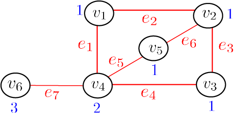
In Figure 1, $\bigcirc_{\mathrm{N}}v_{4}=\{v_{1},v_{3},v_{5},v_{6}\}$ , and graph-based trajectory $g$ satisfies the GL formula $\boldsymbol{\exists_{\mathcal{G}}}\bigcirc_{\mathrm{N}}(g>2)$ only at node $v_{4}$ . For the time interval $I=[1,3]$ , if the node value of node $v_{6}$ stays greater than 2 in the time interval $k+I$ , then the GSTL formula $\lglobally_{[1,3]}(\boldsymbol{\exists_{\mathcal{G}}}\bigcirc_{\mathrm{N}}(g>2))$ is satisfied by graph-based trajectory $g$ at node $v_{4}$ .

III-C Weighted Graph-Based Signal Temporal Logic

An extension of STL is weighted STL (wSTL), where we assign a weight to each subformula of an wSTL formula based on its importance [16][13]. We refer to these weights as importance weights. In this paper, we extend wSTL to weighted GSTL (w-GSTL). In w-GSTL, in addition to defining importance weights for the subformulas, we define the importance weights for both the temporal operators and the GL operators. In other words, we assign an importance weight to each time-step $k\in{I}$ , and we assign an importance weight to each neighbor node $\hat{v}\in\bigcirc_{\mathrm{N}}v$ of a node $v$ . We define the syntax of w-GSTL formulas as follows.

\displaystyle\tilde{\phi}:=\textsuperscript{${w}$}\tilde{\phi}_{\mathcal{G}}\mid\lnot\tilde{\phi}\mid\textsuperscript{${w}_{1}$}\tilde{\phi}^{1}\land\textsuperscript{${w}_{2}$}\tilde{\phi}^{2}\mid\lglobally^{\mathbf{\Omega}}_{I}\tilde{\phi}\mid\leventually^{\mathbf{\Omega}}_{I}\tilde{\phi},

where ${w}_{1}$ and ${w}_{2}$ are positive importance weights on $\textsuperscript{${w}_{1}$}\tilde{\phi}^{1}$ and $\textsuperscript{${w}_{1}$}\tilde{\phi}^{2}$ , respectively; $\mathbf{\Omega}=[{w}_{k_{1}+1},{w}_{k_{1}+2},..,{w}_{k_{2}}]^{T}\in{\real{}^{k_{2}-k_{1}+1}}$ assigns a positive weight ${w}_{k^{\prime}}$ to $k^{\prime}\in[k_{1},k_{2}]$ in the temporal operators; $\boldsymbol{\mathcal{W}}=[{w}_{1},{w}_{2},..,{w}_{|\bigcirc_{\mathrm{N}}v|}]^{T}\in{\real{}^{|\bigcirc_{\mathrm{N}}v|}}$ assigns a positive weight to each $\hat{v}\in\bigcirc_{\mathrm{N}}v$ . In the syntax of w-GSTL formulas, $\textsuperscript{${w}$}\tilde{\phi}_{\mathcal{G}}$ is defined as follows.

	$\displaystyle\textsuperscript{${w}$}\tilde{\phi}_{\mathcal{G}}:=\top\mid\pi\mid\lnot\textsuperscript{${w}$}\tilde{\phi}_{\mathcal{G}}\mid\textsuperscript{${w}_{1}$}\tilde{\phi}^{1}_{\mathcal{G}}\land\textsuperscript{${w}_{2}$}\tilde{\phi}^{2}_{\mathcal{G}}\mid{\boldsymbol{\forall_{\mathcal{G}}}}{\bigcirc_{\mathrm{N}}^{\boldsymbol{\mathcal{W}}}\textsuperscript{}\tilde{\phi}_{\mathcal{G}}}$
	$\displaystyle\mid\boldsymbol{\exists_{\mathcal{G}}}{\bigcirc_{\mathrm{N}}^{\boldsymbol{\mathcal{W}}}\textsuperscript{}\tilde{\phi}_{\mathcal{G}}}$

IVWeighted Graph-Based Signal Temporal Logic and Neural Networks

In this section, we formalize the problem of classifying graph-based trajectories by inferring w-GSTL formulas using neural networks. We denote a set of labeled graph-based trajectories by $\mathcal{D}=\{(g_{i},l_{i})\}^{N_{\mathcal{D}}}_{i=1}$ , and a time horizon by $H=[0,h]$ (where $h\in\mathbb{T}$ ). We assume that the set $\mathcal{D}$ is composed of two subsets: positive subset $\mathcal{D}_{P}=\{g_{i}|l_{i}=+1\}$ which contains the graph-based trajectories representing the desired behavior, and negative subset $\mathcal{D}_{N}=\{g_{i}|l_{i}=-1\}$ which contains the graph-based trajectories representing the undesired behavior. For the cardinality of the defined sets, we have $|\mathcal{D}_{P}|=\tilde{p}$ , $|\mathcal{D}_{N}|=\tilde{n}$ , and $N_{\mathcal{D}}=\tilde{p}+\tilde{n}$ .
Inspired by [17], we define the following.

Definition 1.

We define a w-GSTL formula structure, denoted by $\mathpzc{F}$ , as a w-GSTL formula in which the importance weights of the subformulas and the variables of the atomic predicates, and the importance weights of the GL operators and the temporal operators are replaced by free parameters. In this structure, we assume that we always have at least one temporal operator and one GL operator.

Definition 2.

We define a flexible w-GSTL formula structure $\mathpzc{F}_{\rm{f}}$ as a flexible extension of w-GSTL formula structure such that the types of the temporal operators and the types of the GL operators are to be inferred from data; but the types of the Boolean connectives in the structure are fixed. In this structure, we represent the set of GL operators as a set $P_{\textrm{GL}}=\{{\boldsymbol{\forall_{\mathcal{G}}}},\boldsymbol{\exists_{\mathcal{G}}}\}$ from which the proper operator is to be inferred from data. Similarly, we represent the set of temporal operators as a set $P_{\textrm{temporal}}=\{\leventually^{\mathbf{\Omega}}_{I},\lglobally^{\mathbf{\Omega}}_{I}\}$ .

Example 2.

In the flexible w-GSTL formula structure $\mathpzc{F}_{\rm{f}}:=\textsuperscript{${w}_{1}$}(P_{\textrm{temporal}}^{\mathbf{\Omega}_{1}}(P_{\textrm{GL}}\bigcirc_{\mathrm{N}}^{{\boldsymbol{\mathcal{W}}}}\pi_{1}))\lor$ $\textsuperscript{${w}_{2}$}(P_{\textrm{temporal}}^{\mathbf{\Omega}_{2}}(P_{\textrm{GL}}{\bigcirc_{\mathrm{N}}^{\boldsymbol{\mathcal{W}}}\pi_{2}}))$ , the types of the temporal operators and the GL operators, the importance weights of the subformulas and the variables of the atomic predicates $\pi_{1}$ and $\pi_{2}$ , and the importance weights of the GL operators and the temporal operators are to be inferred from data, but the Boolean connective $\lor$ is fixed.

After determining the proper w-GSTL operators in a given $\mathpzc{F}_{\rm{f}}$ , we obtain a w-GSTL formula $\tilde{\phi}$ that is consistent with $\mathpzc{F}_{\rm{f}}$ .

In order to define the problem statement, we define the classification accuracy, denoted by $AC$ , as $AC={\frac{{\boldsymbol{l}}^{\rm{predicted}}}{N_{\mathcal{D}}}}\times{100}$ , where ${\boldsymbol{l}}^{\rm{predicted}}\in\mathbb{N}$ is the number of correctly classified graph-based trajectories $g_{i}$ .

Problem 1.

Given a set of labeled graph-based trajectories $\mathcal{D}=\{(g_{i},l_{i})\}^{N_{\mathcal{D}}}_{i=1}$ and a flexible w-GSTL formula structure $\mathpzc{F}_{\rm{f}}$ , infer a w-GSTL formula $\tilde{\phi}$ (i.e., select the w-GSTL operators and compute the parameters of that structure) to classify $\mathcal{D}$ such that the classification accuracy $AC$ is maximized.

In order to solve Problem 1, we introduce w-GSTL neural networks (w-GSTL-NN) which combines the characteristics of w-GSTL and neural networks. In the first step, we construct and train a w-GSTL-NN to learn the proper w-GSTL operators in the flexible w-GSTL formula structure $\mathpzc{F}_{\rm{f}}$ . In the second step, we construct and train another w-GSTL-NN to learn the parameters in $\mathpzc{F}_{\rm{f}}$ . In w-GSTL-NN, we combine the activation functions in a neural network with the quantitative satisfaction of w-GSTL. We define the quantitative satisfaction of a w-GSTL formula $\tilde{\phi}$ as follows.

\displaystyle\begin{split}r^{\rm{w}}(g,v,\pi,k)&={f}(g(v,k)),\\ r^{\rm{w}}(g,v,\lnot\tilde{\phi},k)&=-r^{\rm{w}}(g,v,\tilde{\phi},k),\\ r^{\rm{w}}(g,v,{\textsuperscript{${w}_{1}$}\tilde{\phi}^{1}}\land{\textsuperscript{${w}_{2}$}\tilde{\phi}^{2}},k)&=\otimes^{\land}({\{{{w}_{i}},{r^{\rm{w}}(g,v,\tilde{\phi}^{i},k)}\}}_{i=1,2}),\\ r^{\rm{w}}(g,v,{\textsuperscript{${w}_{1}$}\tilde{\phi}^{1}}\lor{\textsuperscript{${w}_{2}$}\tilde{\phi}^{2}},k)&=\otimes^{\lor}({\{{{w}_{i}},{r^{\rm{w}}(g,v,\tilde{\phi}^{i},k)}\}}_{i=1,2}),\\ r^{\rm{w}}(g,v,{\lglobally^{\mathbf{\Omega}}_{I}}\tilde{\phi},k)&=\otimes^{\lglobally}(\mathbf{\Omega},\{r^{\rm{w}}(g,v,\tilde{\phi},i)\}_{i\in{k+I}}),\\ r^{\rm{w}}(g,v,{\leventually^{\mathbf{\Omega}}_{I}}\tilde{\phi},k)&=\otimes^{\leventually}(\mathbf{\Omega},\{r^{\rm{w}}(g,v,\tilde{\phi},i)\}_{i\in{k+I}}),\\ r^{\rm{w}}(g,v,{\boldsymbol{\forall_{\mathcal{G}}}}\bigcirc_{\mathrm{N}}^{\boldsymbol{\mathcal{W}}}\textsuperscript{}\tilde{\phi}_{\mathcal{G}},k)&=\otimes^{{\boldsymbol{\forall_{\mathcal{G}}}}}(\boldsymbol{\mathcal{W}},\{r^{\rm{w}}(g,\hat{v},\textsuperscript{}\tilde{\phi}_{\mathcal{G}},k)\\ &~~~~~~~~~~~~~~~~~~~~~~\}_{\hat{v}\in\bigcirc_{\mathrm{N}}v}),\\ r^{\rm{w}}(g,v,\boldsymbol{\exists_{\mathcal{G}}}\bigcirc_{\mathrm{N}}^{\boldsymbol{\mathcal{W}}}\textsuperscript{}\tilde{\phi}_{\mathcal{G}},k)&=\otimes^{\boldsymbol{\exists_{\mathcal{G}}}}(\boldsymbol{\mathcal{W}},\{r^{\rm{w}}(g,\hat{v},\textsuperscript{}\tilde{\phi}_{\mathcal{G}},k)\\ &~~~~~~~~~~~~~~~~~~~~~~\}_{{\hat{v}\in\bigcirc_{\mathrm{N}}v}}),\end{split}

where $\otimes^{\land},\otimes^{\lor}:\real^{2}_{>0}\times\real^{2}\limplies\real$ , $\otimes^{\lglobally},\otimes^{\leventually}:\real^{k_{2}-k_{1}+1}_{>0}\times\real^{k_{2}-k_{1}+1}\limplies\real$ , and $\otimes^{{\boldsymbol{\forall_{\mathcal{G}}}}},\otimes^{\boldsymbol{\exists_{\mathcal{G}}}}:\real^{|\bigcirc_{\mathrm{N}}v|}_{>0}\times\real^{|\bigcirc_{\mathrm{N}}v|}\limplies\real$ are activation functions corresponding to $\land$ , $\lor$ , $\lglobally^{\mathbf{\Omega}}_{I}$ , $\leventually^{\mathbf{\Omega}}_{I}$ , ${\boldsymbol{\forall_{\mathcal{G}}}}$ , and $\boldsymbol{\exists_{\mathcal{G}}}$ operators, respectively. We denote an activation function with $\otimes^{i}$ , where $i\in{\mathcal{A}}=\{\land,\lor,\lglobally,\leventually,{\boldsymbol{\forall_{\mathcal{G}}}},\boldsymbol{\exists_{\mathcal{G}}}\}$ .

For defining the activation functions, we use the variable $\sigma$ , where $\sigma$ is a positive real number. We define the activation function corresponding to each operator in the set $\mathcal{A}$ as follows.

\displaystyle\begin{split}\otimes^{\land}({\{{{w}_{i}},{r^{\rm{w}}(g,v,\tilde{\phi}^{i},k)}\}}_{i=1,2},\sigma)&=\frac{{\sum}^{2}_{m=1}{\overline{{w}}_{m}s_{m}r_{m}}}{{\sum}^{2}_{m=1}{\overline{{w}}_{m}s_{m}}},\\ \otimes^{\lor}({\{{{w}_{i}},{r^{\rm{w}}(g,v,\tilde{\phi}^{i},k)}\}}_{i=1,2},\sigma)&=-\frac{{\sum}^{2}_{m=1}{\overline{{w}}_{m}s_{m}r_{m}}}{{\sum}^{2}_{m=1}{\overline{{w}}_{m}s_{m}}},\\ \otimes^{\lglobally}(\mathbf{\Omega},\{r^{\rm{w}}(g,v,\tilde{\phi},i)\}_{i\in{k+I}},\sigma)&=\frac{{\sum}^{k_{2}}_{m=k_{1}}{\overline{{w}}_{m}s_{m}r_{m}}}{{\sum}^{k_{2}}_{m=k_{1}}{\overline{{w}}_{m}s_{m}}},\\ \otimes^{\leventually}(\mathbf{\Omega},\{r^{\rm{w}}(g,v,\tilde{\phi},i)\}_{i\in{k+I}},\sigma)&=\frac{{\sum}^{k_{2}}_{m=k_{1}}{\overline{{w}}_{m}s_{m}r_{m}}}{-{\sum}^{k_{2}}_{m=k_{1}}{\overline{{w}}_{m}s_{m}}},\\ \otimes^{{\boldsymbol{\forall_{\mathcal{G}}}}}(\boldsymbol{\mathcal{W}},\{r^{\rm{w}}(g,\hat{v},\textsuperscript{}\tilde{\phi}_{\mathcal{G}},k)\}_{\hat{v}\in\bigcirc_{\mathrm{N}}v},\sigma)&=\frac{{\sum}^{|\bigcirc_{\mathrm{N}}v|}_{m=1}{\overline{{w}}_{m}s_{m}r_{m}}}{{\sum}^{|\bigcirc_{\mathrm{N}}v|}_{m=1}{\overline{{w}}_{m}s_{m}}}\\ \otimes^{\boldsymbol{\exists_{\mathcal{G}}}}(\boldsymbol{\mathcal{W}},\{r^{\rm{w}}(g,\hat{v},\textsuperscript{}\tilde{\phi}_{\mathcal{G}},k)\}_{\hat{v}\in\bigcirc_{\mathrm{N}}v},\sigma)&=\frac{{\sum}^{|\bigcirc_{\mathrm{N}}v|}_{m=1}{\overline{{w}}_{m}s_{m}r_{m}}}{-{\sum}^{|\bigcirc_{\mathrm{N}}v|}_{m=1}{\overline{{w}}_{m}s_{m}}},\\ \end{split}

(2)

where $\overline{{w}}_{m}$ is the normalized weight and $I=[k_{1},k_{2}]$ ; in the activation functions of $\land$ and $\lor$ Boolean connectives, $\overline{{w}}_{m}={w}_{m}/{\sum}^{2}_{j=1}{{w}_{j}}$ ; In the activation functions of $\lglobally^{\mathbf{\Omega}}_{I}$ and $\leventually^{\mathbf{\Omega}}_{I}$ operators, $\overline{{w}}_{m}={w}_{m}/{\sum}^{k_{2}}_{j=k_{1}}{{w}_{j}}$ ; in ${\boldsymbol{\forall_{\mathcal{G}}}}$ and $\boldsymbol{\exists_{\mathcal{G}}}$ graph operators, $\overline{{w}}_{m}={w}_{m}/{\sum}^{|\bigcirc_{\mathrm{N}}v|}_{j=1}{{w}_{j}}$ . $\overline{{w}}_{m}$ aims to normalize the importance weight of the $m$ -th subformula in $\tilde{\phi}$ to the range of $[0,1]$ such that $\overline{w}_{m}$ can reflect the importance of the $m$ -th subformula in determining the quantitative satisfaction of the whole w-GSTL formula $\tilde{\phi}$ . In the activation function of $\land$ operator, $r_{m}=r^{\rm{w}}(g,v,\tilde{\phi}^{m},k)$ ; in the activation function of $\lor$ operator, $r_{m}=-r^{\rm{w}}(g,v,\tilde{\phi}^{m},k)$ ; in the activation function of ${\boldsymbol{\forall_{\mathcal{G}}}}$ operator, $r_{m}=r^{\rm{w}}(g,\hat{v},\textsuperscript{}\tilde{\phi}_{\mathcal{G}},k)$ ; in the activation function of $\boldsymbol{\exists_{\mathcal{G}}}$ operator, $r_{m}=-r^{\rm{w}}(g,\hat{v},\textsuperscript{}\tilde{\phi}_{\mathcal{G}},k)$ ; in the activation function of $\lglobally^{\mathbf{\Omega}}_{I}$ operator, $r_{m}=r^{\rm{w}}(g,v,\tilde{\phi},m)$ ; and in the activation function of $\leventually^{\mathbf{\Omega}}_{I}$ operator, $r_{m}=-r^{\rm{w}}(g,v,\tilde{\phi},m)$ ; in the activation functions of $\land$ and $\lor$ operators, $s_{m}=e^{-\frac{r_{m}}{\sigma}}/{\sum}^{2}_{l=1}{{e^{-\frac{r_{l}}{\sigma}}}}$ ; in the activation functions of $\lglobally^{\mathbf{\Omega}}_{I}$ and $\leventually^{\mathbf{\Omega}}_{I}$ operators, $s_{m}=e^{-\frac{r_{m}}{\sigma}}/{\sum}^{k_{2}}_{l=k_{1}}{{e^{-\frac{r_{l}}{\sigma}}}}$ ; in the activation functions of ${\boldsymbol{\forall_{\mathcal{G}}}}$ and $\boldsymbol{\exists_{\mathcal{G}}}$ operators, $s_{m}=e^{-\frac{r_{m}}{\sigma}}/{\sum}^{|\bigcirc_{\mathrm{N}}v|}_{l=1}{{e^{-\frac{r_{l}}{\sigma}}}}$ .

VMethodology

In this section, we introduce a framework and algorithms to solve Problem 1 for a given flexible w-GSTL formula structure $\mathpzc{F}_{\rm{f}}$ with $M$ undetermined temporal operators and $L$ undetermined GL operators using w-GSTL-NN. For the training of w-GSTL-NN, we design a loss function to meet the following two requirements: 1) the loss should be small when the inferred formula is satisfied by graph-based trajectories in $\mathcal{D}^{P}$ and violated by the graph-based trajectories in $\mathcal{D}^{N}$ ; 2) the loss should be large when the inferred formula is not satisfied by the graph-based trajectories in $\mathcal{D}^{P}$ and not violated by the graph-based trajectories in $\mathcal{D}^{N}$ . We define the loss function as follows.

J(\tilde{\phi})={\sum\limits^{N_{\mathcal{D}}}_{i=1}{e^{-\eta l_{i}r^{\rm{w}}(g_{i},\tilde{\phi})}}},

(3)

where $g_{i}$ denotes the $i$ -th graph-based trajectory in $\mathcal{D}$ , and $\eta>0$ is a tuning parameter. $J(\tilde{\phi})$ is small for the cases where $l_{i}r^{\rm{w}}(g_{i},\tilde{\phi})>0$ and increases exponentially when $l_{i}r^{\rm{w}}(g_{i},\tilde{\phi})<0$ .

Input: a set of labeled graph-based trajectories

\mathcal{D}

w-GSTL structure

\mathpzc{F}_{\rm{f}}

number of iterations

K

number of subformulas

\mathcal{J}

Output: Learned w-GSTL formula

\tilde{\phi}

Construct a w-GSTL-NN based on the given structure

\mathpzc{F}_{\rm{f}}

Initialize

\boldsymbol{w}^{\mathpzc{F}_{\rm{f}}}

\mathbf{a_{S}}

and

{c}

Initialize

\{b_{i}\}^{M}_{i=1}

\{b^{\prime}_{i^{\prime}}\}^{L}_{i=1}

, respectively corresponding to

P_{\textrm{temporal}}

and

P_{\textrm{GL}}

\{b_{i}\}^{M}_{i=1},\{b^{\prime}_{i^{\prime}}\}^{L}_{i^{\prime}=1}\leftarrow

w-GSTL-NN(

\mathcal{D},\mathpzc{F}_{\rm{f}},K,\mathcal{J},\{\{b_{i}\}^{M}_{i=1},\{b^{\prime}_{i^{\prime}}\}^{L}_{i^{\prime}=1}\})

for $i=1,...,M$ do 10

if $b_{i}\geq{0}$ then

b_{i}\leftarrow{q_{\lglobally}}

else

b_{i}\leftarrow{q_{\leventually}}

end for 14

for $i^{\prime}=1,...,L$ do 15

if $b^{\prime}_{i^{\prime}}\geq{0}$ then

b^{\prime}_{i^{\prime}}\leftarrow{q_{{\boldsymbol{\forall_{\mathcal{G}}}}}}

else

b^{\prime}_{i^{\prime}}\leftarrow{q_{\boldsymbol{\exists_{\mathcal{G}}}}}

end for 19

\mathpzc{F}\leftarrow

Selected operators from the

P_{\textrm{GL}}

and the

P_{\textrm{temporal}}

\boldsymbol{w}^{\mathpzc{F}_{\rm{f}}},\mathbf{a_{S}},{c}\leftarrow

w-GSTL-NN(

\mathcal{D},\mathpzc{F},K,\mathcal{J},\{\boldsymbol{w}^{\mathpzc{F}_{\rm{f}}},\mathbf{a_{S}},{c}\})

\tilde{\phi}\leftarrow{\boldsymbol{w}}^{\mathpzc{F}_{\rm{f}}},\mathbf{a_{S}},{c}

return $\tilde{\phi}$ 25

Algorithm 1 Two-step procedure of inferring a w-GSTL formula

We compute a w-GSTL formula in two steps: 1) determining the proper temporal and GL operators in the given flexible w-GSTL formula structure $\mathpzc{F}_{\rm{f}}$ ; 2) learning the parameters of the flexible w-GSTL formula structure $\mathpzc{F}_{\rm{f}}$ . For each step, we construct and train a separate w-GSTL-NN.

Algorithm 1 illustrates the two-step procedure of learning a w-GSTL formula from a given set of labeled graph-based trajectories $\mathcal{D}$ and a given flexible w-GSTL formula structure $\mathpzc{F}_{\rm{f}}$ .

Step 1

In step 1, we initialize two sets of coefficients: (a) $\{b_{i}\}^{M}_{i=1}$ corresponding to $M$ undetermined temporal operators; (b) $\{b^{\prime}_{i^{\prime}}\}^{L}_{i^{\prime}=1}$ corresponding to $L$ undetermined GL operators, where $b_{i},b^{\prime}_{i^{\prime}}\in\real$ (Line 3 in Alg. 1). In this step, for the activation functions of $\lglobally^{\mathbf{\Omega}}_{I}$ and $\leventually^{\mathbf{\Omega}}_{I}$ , we define the coefficients $q_{\lglobally}=+1$ and $q_{\leventually}=-1$ , respectively. Similarly, for the activation functions of ${\boldsymbol{\forall_{\mathcal{G}}}}$ and $\boldsymbol{\exists_{\mathcal{G}}}$ , we define the coefficients $q_{{\boldsymbol{\forall_{\mathcal{G}}}}}=+1$ $q_{\boldsymbol{\exists_{\mathcal{G}}}}=-1$ , respectively. We construct and train a w-GSTL-NN (demonstrated in Alg. 2) to learn $\{b_{i}\}^{M}_{i=1}$ and $\{b^{\prime}_{i^{\prime}}\}^{L}_{i^{\prime}=1}$ (Line 4 in Alg. 1). For each undetermined temporal operator, the sign of the returned $b_{i}$ determines the proper selection from the set $P_{\textrm{temporal}}$ . In other words, if $b_{i}\geq{0}$ , then we have $b_{i}=q_{\lglobally}$ . This means the proper selection for the temporal operator corresponding to $b_{i}$ is $\lglobally^{\mathbf{\Omega}}_{I}$ . If $b_{i}<{0}$ , then $\leventually^{\mathbf{\Omega}}_{I}$ is the proper selection from the set $P_{\textrm{temporal}}$ (Line 5 to 8 in Alg. 1). Similarly, for each undetermined GL operator, the sign of the returned $b^{\prime}_{i^{\prime}}$ determines the proper selection of the undetermined GL operator from the set $P_{\textrm{GL}}$ (Lines 9 to 12 in Alg. 1).

Input: a set of labeled graph-based trajectories

\mathcal{D}

flexible w-GSTL formula structure structure

\mathpzc{F}_{\rm{f}}

(or a formula structure

\mathpzc{F}

)
number of iterations

K

number of subformulas

\mathcal{J}

Output:

Parameters

\{b_{i}\}^{M}_{i=1}

and

\{b_{i^{\prime}}\}^{L}_{i^{\prime}=1}

, and the parameters of

\mathpzc{F}_{\rm{f}}

Construct a w-GSTL-NN based on the given structure

\mathpzc{F}_{\rm{f}}

for $k=$ 1, 2, …, $K$ do 6

Select a mini-batch data

\mathcal{D}^{k}

from

\mathcal{D}

for $j=$ 1, 2, …, $\mathcal{J}$ do 8

Parameters\leftarrow{F_{\textrm{forward}}(\mathcal{D}^{k},\mathit{subf(j)},\otimes^{j},Parameters)}

end for 11

Compute

J(\tilde{\phi})

using (3) 13

Parameters\mbox{~and~}r^{\rm{w}}(g_{i},\tilde{\phi})\leftarrow{F_{\textrm{backward}}(\mathcal{D}^{k},Parameters,{J(\tilde{\phi})})}

end for 16

return $Parameters$

Algorithm 2 w-GSTL-NN: neural network for learning w-GSTL formulas

Step 2

After determining the proper operators, we construct and train another w-GSTL-NN (demonstrated in Alg. 2) to learn parameters of the flexible w-GSTL formula structure $\mathpzc{F}_{\rm{f}}$ including $\mathbf{a_{S}}$ , ${c}$ , and all the importance weights in the flexible w-GSTL formula structure $\mathpzc{F}_{\rm{f}}$ that we denote them by $\boldsymbol{w}^{\mathpzc{F}_{\rm{f}}}$ (Lines 13 to 16 in Alg. 2).

Algorithm 2 illustrates w-GSTL-NN that we use to learn w-GSTL formulas. In Algorithm 2, $Parameters$ denotes a set of parameters that we calculate at each step of the two-step process of learning a w-GSTL formula. In step 1, $Parameters$ includes $\{b_{i}\}^{M}_{i=1}$ and $\{b_{i^{\prime}}\}^{L}_{i^{\prime}=1}$ . In step 2, $Parameters$ includes the parameters of the flexible w-GSTL formula structure $\mathpzc{F}_{\rm{f}}$ (including $\mathbf{a_{S}}$ , ${c}$ , and $\boldsymbol{w}^{\mathpzc{F}_{\rm{f}}}$ ). In Algorithm 2, we denote the forward-propagation operation by $F_{\textrm{forward}}(\mathcal{D}^{k},\mathit{subf(j)},\otimes^{i},Parameters)$ , where $\mathcal{D}^{k}$ denotes the selected mini-batch from the set $\mathcal{D}$ , $\mathit{subf(j)}$ is the $j$ th subformula in $\mathpzc{F}_{\rm{f}}$ , $\otimes^{j}$ is activation function corresponding to the w-GSTL operator or Boolean connective in $\mathit{subf(j)}$ , $Parameters$ is to be calculated, and $r^{\rm{w}}(g_{i},\tilde{\phi})$ is the output of forward-propagation (Line 5 in Alg. 2). More clearly, after determining the w-GSTL operators, w-GSTL-NN calculates the quantitative satisfaction of the inferred $\tilde{\phi}$ with respect to $g_{i}$ through forward-propagation. Also, We denote the back-propagation operation by $F_{\textrm{backward}}(\mathcal{D}^{k},Parameters,J(\tilde{\phi}))$ , where $Parameters$ is to be updated (Line 8 in Alg. 2). The proposed algorithms are implemented in a Python toolbox¹¹ 1 https://github.com/kazhirota7/Graph-based-wSTLNN.

The time complexity for learning a w-GSTL-NN for a given graph $G(V,E)$ is $\mathcal{O}({u_{1}}{u_{2}}{u_{3}}{n_{E}}{u_{4}})$ , where $u_{1}$ is the number of training samples, $u_{2}$ is the number of graph-based trajectories in each sample, $u_{3}$ is the number of epochs, $n_{E}$ is the number of nodes in the graph $G(V,E)$ , and $u_{4}$ is the total number of temporal and graph-based operators in the flexible w-GSTL formula structure $\mathpzc{F}_{\rm{f}}$ .

VICase Studies

In this section, we assess the performance of w-GSTL-NN. We first use a meteorological dataset in Australia to predict rainfall. Then, we predict the severity of lockdown measures using COVID-19 data in Italy. The performance of w-GSTL-NN is compared with some other standard classification algorithms. The flexible w-GSTL formula structure that we use for these two case studies is $\mathpzc{F}_{\rm{f}}:=\textsuperscript{${w}_{1}$}(P_{\textrm{temporal}}^{\mathbf{\Omega}_{1}}(P_{\textrm{GL}}\bigcirc_{\mathrm{N}}^{{\boldsymbol{\mathcal{W}}}}\pi_{1}))\lor(\lnot\textsuperscript{${w}_{2}$}($ $(P_{\textrm{temporal}}^{\mathbf{\Omega}_{2}}P_{\textrm{GL}}{\bigcirc_{\mathrm{N}}^{\boldsymbol{\mathcal{W}}}\pi_{2}})))$ . For both case studies, we use the Adam optimization algorithm [18] to learn the neural network. The ${c}$ parameter is initialized as 0 to prevent initial bias. Furthermore, all of the importance weights are initialized at the same value of 0.5, also to prevent initial bias.

VI-A Case Study I: Rain Prediction

In this subsection, we use w-GSTL-NN to predict rainfall in regions of Australia. The dataset is acquired from the Australian Government Bureau of Meteorology²² 2 http://www.bom.gov.au/climate/data/[19]. The dataset that we use is composed of weather-related data in 49 regions of Australia measured daily from March 1st, 2013 to June 25th, 2017, including minimum sunshine ( $g^{1}$ ), cloud at 9am ( $g^{2}$ ), cloud at 3pm ( $g^{3}$ ), and whether there was any rain on the given day (-1 or 1) ( $g^{4}$ ). Only the most important attributes are mentioned due to space limitations. The criterion for the binary classification is the rain prediction for the following day (-1 for no rain, 1 for rain). We construct a graph structure of the Australian regions, considering any region within a 300 km radius of another region to be neighbors. A separate neural network is learned for each region and its neighbors to prevent scalability issues when broader regions are considered. We utilize the zero imputation method for missing values in the input data. The dataset is divided into a proportion of 0.8:0.2 for the training dataset and testing dataset, respectively, resulting in 1262 total data points per region for the training dataset and 316 total data points per region for the testing dataset.

For a demonstration of how the importance weights and predicates can be interpreted, we consider the learned neural network for Albury and its neighbors: Wagga Wagga, Canberra, Tuggeranong, Mount Ginini, Bendigo, Sale, Melbourne Airport, Melbourne, and Watsonia. We set $K_{I}$ consecutive days of data as one instance of the dataset in our experiment. The dataset is passed through two separate neural networks. In the first step, we determine the temporal operators and the GL operators to be applied on $I_{i}$ and $I_{ii}$ intervals, respectively. In the second step, we learn the parameters of the flexible w-GSTL formula structure $\mathpzc{F}_{\rm{f}}$ .

In the experiment, we set $K_{I}$ = 15, $I_{i}$ = [0, 6], $I_{ii}$ = [7, 14], $\eta$ = 1, and $\sigma$ = 1. The learned w-GSTL formula is $\tilde{\phi}=\textsuperscript{${w}_{1}$}(\lglobally^{\mathbf{\Omega}_{1}}_{[0,6]}(\boldsymbol{\exists_{\mathcal{G}}}{\bigcirc_{\mathrm{N}}}^{\boldsymbol{\mathcal{W}}}\pi))\lor(\lnot\textsuperscript{${w}_{2}$}(\leventually^{\mathbf{\Omega}_{2}}_{[7,14]}(\boldsymbol{\exists_{\mathcal{G}}}{\bigcirc_{\mathrm{N}}^{\boldsymbol{\mathcal{W}}}}\pi)))$ , and the inferred predicate $\pi$ is $\pi:=-0.0298g^{1}+0.0226g^{2}+0.0222g^{3}-0.0309g^{4}\leq 0.6593)$ , the importance weights for $I_{i}$ are³³ 3 The importance weights for $I_{ii}$ were omitted due to space limitation. $\mathbf{\Omega}_{1}=[0.1087,0.2210,0.0655,0.1927,0.0163,0.1349,0.2609]$ , the normalized importance weights for Wagga Wagga, Canberra, Tuggeranong, Mount Ginini, Bendigo, Sale, Melbourne Airport, Melbourne, and Watsonia, respectively, are $\boldsymbol{\mathcal{W}}=[0.0443,0.1439,0.0319,0.1930,0.1299,0.0000,0.1984,\\ 0.1719,0.0867]$ , and the normalized importance weights for the $\lor{}$ operator are: ${w}_{1}$ = 0.6891, ${w}_{2}$ = 0.3109.

We evaluate the performance of the proposed algorithm by applying some standard classification methods such as K-nearest neighbors (KNN) and decision tree (DT), kernel method such as support vector machine (SVM), and an artificial neural network (ANN) algorithm on the same dataset.

Method	Obtained Accuracy
	for the Test Dataset (%)
Decision Tree	76.14
K-Nearest Neighbors (KNN)	81.04
Support Vector Machine (SVM)	82.61
ANN (Sequential Model)	84.73
w-GSTL-NN (this paper)	81.69

TABLE I: Obtained classification accuracy on the rainfall test dataset of 49 Australian regions.

w-GSTL-NN produces a higher accuracy than both KNN and DT (Table I). Although SVM and ANN produce higher accuracy than w-GSTL-NN because they are not restricted by the w-GSTL formula, w-GSTL-NN can generate human-readable results, unlike the other algorithms. Using the learned w-GSTL formula, the learned importance weights, and the predicates, we can interpret the decision-making of the classifier, rather than merely interpreting the results generated by a black box. The signs and the magnitudes of the predicates can be used to analyze the correlation between each meteorological input and rain prediction. The greater magnitude of the predicate suggests a stronger correlation between the input and rain prediction, and the sign of the predicate indicates whether the input has a positive or a negative relationship with rain prediction. For instance, the coefficients associated with the predicates suggest that larger amount of clouds at 9 am ( $g^{2}$ ), a larger amount of clouds at 3 pm( $g^{3}$ ), and more rainfall during the interval ( $g^{4}$ ) in the input data correlates to a larger probability that there will be rainfall on the target date, while the larger amount of sunshine ( $g^{1}$ ) correlates to a larger probability that there will not be rainfall on the target date. Furthermore, the learned importance weights associated with $\boldsymbol{\exists_{\mathcal{G}}}$ suggest that the meteorological conditions in Mount Ginini and Melbourne Airport are the best indicators for predicting rain in Albury.

VI-B Case Study II: Classifying COVID-19 Lockdown Measures

In this subsection, we use simulated COVID-19 datasets of 20 Italian regions from the DiBernardo Group Repository[20]. The dataset is composed of a time-series dataset for each region in Italy. The inputs of each time series are percentage of people infected ( $g^{1}$ ), quarantined ( $g^{2}$ ), deceased ( $g^{3}$ ), and hospitalized due to COVID-19 ( $g^{4}$ ). The data is simulated for the social distancing parameter of 0.3 for strict lockdown measures and 1 for no lockdown measures. Each of the inputs of the data was recorded daily for 365 days. We turn this case study into a binary classification by labeling “strict lockdown measures” with -1 and “no lockdown measures” with 1. For the demonstration of the learned importance weights and predicates, we consider the learned spatial-temporal properties of Abruzzo and its neighboring regions: Lazio, Marche, and Molise.

In this case study, we use $K_{I}$ = 30, $I_{i}$ = [0, 14], $I_{ii}$ = [15, 29], $\eta$ = 1, and $\sigma$ = 1. We divide the dataset into 472 sets of $K_{I}$ time instances for training dataset and 200 sets of $K_{I}$ time instances for testing dataset. The w-GSTL formula with learned operators is $\tilde{\phi}=\textsuperscript{${w}_{1}$}(\lglobally^{\mathbf{\Omega}_{1}}_{[0,14]}(\boldsymbol{\exists_{\mathcal{G}}}\bigcirc_{\mathrm{N}}^{{\boldsymbol{\mathcal{W}}}}\pi))\lor(\lnot\textsuperscript{${w}_{2}$}(\leventually^{\mathbf{\Omega}_{2}}_{[15,29]}(\boldsymbol{\exists_{\mathcal{G}}}\bigcirc_{\mathrm{N}}^{{\boldsymbol{\mathcal{W}}}}\pi)))$ , where the inferred predicate $\pi$ is $\pi:=(-4.4617g^{1}-4.3504g^{2}-3.2291g^{3}-4.4045g^{4}\leq-0.1421)$ , the normalized importance weights for $I_{ii}$ are $\mathbf{\Omega}_{2}=[0.0006,0.0007,0.0008,0.0008,0.0007,0.0008,0.0007,\\ 0.0007,0.0007,0.0006,0.0007,0.0008,0.0007,0.1663,0.8064]$ , the normalized importance weights for Lazio, Marche, and Molise, respectively, are $\boldsymbol{\mathcal{W}}=[0.0002,0.0001,0.9997]$ , and the normalized importance weights for the $\lor{}$ operator are: ${w}_{1}$ = 0.9998, ${w}_{2}$ = 0.0002.

We apply the K-nearest neighbors, decision tree, and support vector machine algorithms on this dataset to conduct the binary classification. The learned w-GSTL formula provides us with the spatial-temporal properties of the dataset and determines whether there is a strict lockdown measure in the region or not. Furthermore, the accuracy of w-GSTL-NN matches that of K-nearest neighbors, decision tree, and support vector machine for the COVID-19 test dataset, all achieving an accuracy of 100%. Nevertheless, w-GSTL-NN provides important information for analysis that would not be possible to retrieve when using other algorithms, which makes w-GSTL-NN useful for applications when interpretation for the decision-making of computers is necessary.

VIIConclusion

In this paper, we proposed a framework that combined neural networks and w-GSTL for learning spatial-temporal properties from data. The proposed approach represents the learned knowledge in a human-readable form. As the future direction, we plan to extend this approach to scenarios where only the positive data is available. Also, we aim to apply w-GSTL-NN in the settings of deep reinforcement learning (deep RL) to improve the interpretability of the deep RL, where we deal with graph-structured problems.

References

[1] S. Seshia and D. Sadigh, “Towards verified artificial intelligence,” ArXiv, vol. abs/1606.08514, 2016.
[2] Z. Xu, A. J. Nettekoven, A. Agung Julius, and U. Topcu, “Graph Temporal Logic Inference for Classification and Identification,” Proceedings of the IEEE Conference on Decision and Control, vol. 2019-December, pp. 4761–4768, 2019.
[3] I. Haghighi, S. Sadraddini, and C. Belta, “Robotic swarm control from spatio-temporal specifications,” 2016 IEEE 55th Conference on Decision and Control, CDC 2016, no. Cdc, pp. 5708–5713, 2016.
[4] F. Djeumou, Z. Xu, and U. Topcu, “Probabilistic swarm guidance subject to graph temporal logic specifications,” in Robotics: Science and Systems, 2020.
[5] J. E. Hopcroft and J. D. Ullman, Introduction to Automata Theory, Languages, and Computation. Addison-Wesley Publishing Company, 1979.
[6] L. Alexis and et. al., “Formalizing trajectories in human-robot encounters via probabilistic stl inference,” IEEE/RSJ International Conference on Intelligent Robots and Systems (IROS), 2021.
[7] I. Gühring, M. Raslan, and G. Kutyniok, “Expressivity of Deep Neural Networks,” ArXiv, pp. 1–37, 2020. [Online]. Available: http://arxiv.org/abs/2007.04759
[8] Z. Liu, M. Jiang, and H. Lin, “A graph-based spatial temporal logic for knowledge representation and automated reasoning in cognitive robots,” ArXiv, pp. 1–15, 2020. [Online]. Available: http://arxiv.org/abs/2001.07205
[9] Y. Seo, M. Defferrard, P. Vandergheynst, and X. Bresson, “Structured sequence modeling with graph convolutional recurrent networks,” in Neural Information Processing, L. Cheng, A. C. S. Leung, and S. Ozawa, Eds. Cham: Springer International Publishing, 2018, pp. 362–373.
[10] Z. Wu, S. Pan, G. Long, J. Jiang, and C. Zhang, “Graph wavenet for deep spatial-temporal graph modeling,” IJCAI International Joint Conference on Artificial Intelligence, vol. 2019-Augus, pp. 1907–1913, 2019.
[11] E. Asarin, A. Donzé, O. Maler, and D. Nickovic, “Parametric identification of temporal properties,” in Runtime Verification, S. Khurshid and K. Sen, Eds. Berlin, Heidelberg: Springer Berlin Heidelberg, 2012, pp. 147–160.
[12] A. Ziat, E. Delasalles, L. Denoyer, and P. Gallinari, “Spatio-temporal neural networks for space-time series forecasting and relations discovery,” Proceedings - IEEE International Conference on Data Mining, ICDM, vol. 2017-November, pp. 705–714, 2017.
[13] R. Yan and A. Julius, “Neural network for weighted signal temporal logic,” ArXiv, 2021. [Online]. Available: http://arxiv.org/abs/2104.05435
[14] L. Serafini and A. Garcez, “Logic tensor networks: Deep learning and logical reasoning from data and knowledge,” ArXiv, vol. abs/1606.04422, 2016.
[15] R. Riegel, A. Gray, F. Luus, N. Khan, N. Makondo, I. Y. Akhalwaya, H. Qian, R. Fagin, F. Barahona, U. Sharma, S. Ikbal, H. Karanam, S. Neelam, A. Likhyani, and S. Srivastava, “Logical neural networks,” ArXiv, 6 2020. [Online]. Available: http://arxiv.org/abs/2006.13155
[16] N. Mehdipour, C. I. Vasile, and C. Belta, “Specifying User Preferences Using Weighted Signal Temporal Logic,” IEEE Control Systems Letters, vol. 5, no. 6, pp. 2006–2011, 2021.
[17] Z. Kong, A. Jones, and C. Belta, “Temporal Logics for Learning and Detection of Anomalous Behavior,” IEEE Transactions on Automatic Control, vol. 62, no. 3, pp. 1210–1222, 2017.
[18] D. P. Kingma and J. Ba, “Adam: A method for stochastic optimization,” in 3rd International Conference on Learning Representations, ICLR 2015, 2015. [Online]. Available: http://arxiv.org/abs/1412.6980
[19] J. Young and A. Young, “Rain in australia,” Kaggle, 12 2017. [Online]. Available: https://www.kaggle.com/jsphyg/weather-dataset-rattle-package
[20] R. Della and et. al., “A network model of italy shows that intermittent regional strategies can alleviate the covid-19 epidemic,” Nature Communications, vol. 11, no. 5106, 10 2020.