A New Estimator for Phase Statistics
Abstract
We introduce a novel statistic to probe the statistics of phases of Fourier modes in two-dimensions (2D) for weak lensing convergence field . This statistic contains completely independent information compared to that contained in observed power spectrum. We compare our results against state-of-the-art numerical simulations as a function of source redshift and find good agreement with theoretical predictions. We show that our estimator can achieve better signal-to-noise compared to the commonly employed statistics known as the line correlation function (LCF). Being a two-point statistics, our estimator is also easy to implement in the presence of complicated noise and mask, and can also be generalised to higher-order. While applying this estimator for the study of lensed CMB maps, we show that it is important to include post-Born corrections in the study of statistics of phase.
1 Introduction
The weak lensing surveys which include Canada-France-Hawaii Telescope(CFHTLS)11 1 http://www.cfht.hawai.edu/Sciences/CFHLS, PAN-STARRS22 2 http://pan-starrs.ifa.hawai.edu/, Dark Energy Surveys (DES)33 3 https://www.darkenergysurvey.org/[1], Prime Focus Spectrograph44 4 http://pfs.ipmu.jp, WiggleZ55 5 http://wigglez.swin.edu.au/[2], BOSS66 6 http://www.sdss3.org/surveys/boss.php[3], KiDS[4] and Subaru Hypersuprimecam survey77 7 http://www.naoj.org/Projects/HSC/index.html(HSC) [5] are already providing important cosmological insights. The future large scale structure (LSS) surveys Euclid88 8 http://sci.esa.int/euclid/[6], Rubin Observatory99 9 http://www.lsst.org/llst home.shtml[7] and Roman Space Telescope1010 10 https://roman.gsfc.nasa.gov/ list weak lensing as their main science driver and are expected to take us beyond the standard model of cosmology [8] by answering some of the most profound questions regarding the nature of dark matter and dark energy (equivalently the modified theories of gravity)[9, 10] and nature of neutrino mass hierarchy [11].
Weak lensing observations target the low-redshift universe and small scales where the perturbations are in the nonlinear regime and statistics are non-Gaussian [12]. Many different estimators exist which probe the higher-order statistics of weak lensing maps [13]. These include the well known real-space one-point statistics such as the cumulants [14] or their two-point correlators also known as the cumulant correlators as well as the associated PDF [15] and the peak-count statistics [16]. In the harmonic domain the estimators such as the Skew-Spectrum[17], Integrated Bispectrum [18] kurt-spectra [19], morphological estimator [20], integrated tripsectrum [21], Betti number [22], extreme value statistics [23], position-dependent PDF [24], density split statistics [25], response function formalism [26] estimators for shapes of the lensing bispectrum [27] are some of the statistical estimators and formalism recently considered by various authors in the context of understanding cosmological statistics in general and weak lensing in particular.
The gravitational clustering in the quasilinear and nonlinear regime generates coupling of Fourier modes that results in correlation of their phases [28]. The power spectrum does not contain any phase information [29]. Notable initial work on statistical evolution of phases of the Fourier modes in gravitational clustering in the quasilinear regime can be found in [30, 31]. These studies relied on a perturbative framework and were tested against numerical simulations [32]. A universal behavior in evolution of phases of the Fourier modes in the nonlinear regime was reported in [33].
In recent years an estimator known also as the line correlation function (LCF) to measure for three-point (third-order) phase correlations was introduced in [34] (also see [35]). This was used in many different contexts. The possibility of improving the cosmological constraints using phase correlations were studied in [36, 37]. In the context of redshift-space distortions this was used in [38]. The growth rate of perturbation were probed in [39]. One of the motivation in this paper is to introduce the third-order phase correlation functions for projected surveys in general and weak lensing surveys in particular. We introduce third-order estimators using both two- and three-point statistics.
We note here in passing that in addition to the summary statistics listed above, in recent years many novel techniques have gained popularity. These include Bayesian hierarchical modelling, likelihood-free or forward modelling approaches. However, it is important to realise that many of these methods often rely on simulations that are based on lognormal approximation or high-order Lagrangian theories and are only approximate compared to accurate ray tracing simulations which can be rather expensive (however, see also [40, 41]).
At leading order the LCF takes contributions from the bispectrum. However, at smaller separations, it also take contribution from higher-order statistics. The perturbative treatment breaks down at smaller separation. The LCF encodes information that is highly complementary to that contained in the power spectrum. Next, we will introduce a two-point statistics also known as cumulant-correlator which can probe phase bispectrum with a higher signal-to-noise.
The LCF has also been employed to distinguish various morphological types of collapsed objects [35]. In addition to the LCF other real space triangular configurations (TCF) have been considered for the study of third-order phase statistics, e.g., [42] employed TCF to probe the characteristic scale of ionized regions during the epoch of reionization from cm interferometric observations.
2 Weak Lensing Bispectrum
The projected weak lensing convergence is a line-of-sight integration of the underlying three-dimensional (3D) cosmological density contrast . The at a position can be expressed as follows:
| (2.1) |
Here is the comoving angular diameter distance at a comoving distance . The kernel encodes geometrical dependence; is the scale factor, is the hubble constant and is the cosmological density parameter. and are comoving angular diameter distances at a comoving distances and . We have assumed all sources to be at a single source plane at a distance .
The power spectrum and the bispectrum for the convergence maps are defined through the following expression :
| (2.2a) | |||
| (2.2b) | |||
The two dimensional Fourier transform of is denoted as with being the two-dimensional wave vector. we denote the two-dimensional Dirac delta function as . We will use and to denote the power spectrum and bispectrum respectively of the underlying three dimensional cosmological density contrast . In the tree level standard perturbation theory the bispectrum can be expressed in terms of the kernel and power spectrum as follows [28]:
| (2.3a) | |||
| (2.3b) | |||
The perturbative bispectrum as which depends on the linear power spectrum . Here, represents 3D wave vectors and their moduli are represented as . In the flat-sky approximation, the convergence power spectrum and bispectrum can be expressed in terms of the underlying power spectrum and using the following line-of-sight integrations:
| (2.4a) | |||
| (2.4b) | |||
In the highly nonlinear regime many different halo-model based fitting functions have been proposed. We will use the most recent fitting function presented in Ref.[43] known to be more accurate compared to the previous fitting functions. We will use these expressions in our calculation for the Line Correlation Function (LCF) for the field. Notice that bispectrum only represents the leading contribution. Higher-order correction also get contributions from higher-order statistics such as the trispectrum which we have ignored in our study,
For the validation of our theoretical results we use simulation that adopted cosmological parameters consistent with the WMAP 9 year result , , , , and
3 Third-order Phase Statistics in Projection
We will introduce the two-point correlation function of the weak lensing convergence through the following expression:
| (3.1) |
Here is the Legendre polynomial and represents the angular harmonics. Also, represents the Bessel Function of order zero of the first kind. The angular power spectrum of convergence is identical to for the flat-sky approximation. We will specialise the discussion to weak lensing convergence in the following section, For the purpose of discussion here is a generic two-dimensional (2D) field defined over the celestial sphere. We will consider a flat patch of the sky for our discussion. The position vector is defined using the polar angle and Cartesian unit vectors and :
| (3.2) |
Next we will consider two third-order statistics in projection.
3.1 Line Correlation Function in Projection
We will denote the LCF as which is defined through the following expression as a function of the angular scale is
| (3.3) |
The LCF is a angle-averaged three-point collapsed correlation function where the three-points are in a collinear configuration. The two outer points are equidistant from the central point situated at at a distance . represents the survey area. Assuming isotropy and homogeneity the estimator depends only on the separation angular scale and does not depend on the position angle . We consider the following convention for the Fourier transform relating and . Where, is a real field constructed from the phases of the convergence map and is constructed from the and its amplitude , i.e., . The two-dimensional wave vector is denoted by . Then
| (3.4) |
The represents the smoothing window. We will not consider observational mask. The real-space statistics can be estimated simply by avoiding the masked region. The three-point correlation function of can be expressed as follows:
| (3.5) |
The LCF in terms of the bispectrum can be expressed as follows:
| (3.6) |
The three-point correlation function of the phase can be written in terms of the convergence bispectrum
| (3.7) |
Using Eq.(3.7) in Eq.(3.3) we arrive at the following expression:
| (3.8a) | |||
| (3.8b) | |||
We have used the following Bessel’s first integral1111 11 Bessel’s first integral (Eq.(71) of Mathsworld) to reduce Eq.(3.8a).
| (3.9) |
Here, denotes the Bessel functions of the first kind of order .
In addition to the LCF of phases introduced in Eq.(3.8a)-Eq.(3.8b) we will also consider the following associated estimator:
| (3.10a) | |||
| (3.10b) | |||
The derivation of Eq.(3.10b) follows the same steps as the derivation of Eq.(3.8b).
The Effective Field Theory (EFT) provides a framework to extend the SPT results to smaller scales. Including the additional counter-terms from EFT in the expression of the kernel will extend the validity of results based on SPT to smaller angular scales not just for gravity induced non-Gaussianity but also for primordial non-Gaussianity [45].
3.2 Cumulant Correlators of Phases in Projection
The line correlation function considers a collapsed configuration of a triangle with equidistant points from the central location. The other collapsed configuration that is commonly used in the literature was introduced in [47] in the context of density contrast in and are known as the cumulant correlators. The two-to-one correlator defined below is of the lowest-order in the family of cumulant correlators and can be constructed cross-correlating a squared map with itself:
| (3.11) |
Here is the skew-spectrum of the map constructed from its bispectrum
| (3.12a) | |||
Here denotes the cosine of the angle betwwn and i.e. with . Here the quantity in parentheses is the well-known Wigner- symbol. For more detailed derivation of flat-sky vs. all-sky correspondence see Appendix-§A. In Appendix-§B. we have presented generalisation to higher-order.
The interest in cumulant correlators stems from the fact that they are two-point correlations but carry information about three-point statistics. They can be generalised easily to higher order. The information content is in general different for various triangular configurations. For an equilateral configuration see [42].
4 Results and Discussion
In this section we will discuss the results of our numerical investigations for various estimators and compare them against theoretical predictions.
Maps: To validate our analytical results we use the publicly available all-sky weak lensing maps generated by [44]1212 12 http://cosmo.phys.hirosaki-u.ac.jp/takahasi/allsky_raytracing/. The ray-tracing through N-body simulations were used to generate these maps. These simulation used particles to follow the evolution of gravitational clustering. To generate the convergence and the corresponding shear maps multiple lens planes were used; the source redshifts used were in the range . We have chosen the maps with for our study. For CMB maps the lensing potentials were constructed using the deflection angles which were used to construct the lensing potentials and eventually the maps. These maps include post-Born corrections. Importance of post-Born terms in lensing statistics in the context of CMB studies were outlined [48]. However, recent studies have shown such corrections are not important in case of weak lensing statistics which probe lower redshifts. The convergence maps were generated using an equal area pixelisation scheme in HEALPix1313 13 https://healpix.jpl.nasa.gov/ format[49].
The set of maps we use in this study are generated at and were cross-checked against higher resolution maps constructed at a higher resolution for consistency. These maps constructed at different resolution were found to be consistent with each other up to the angular harmonics .
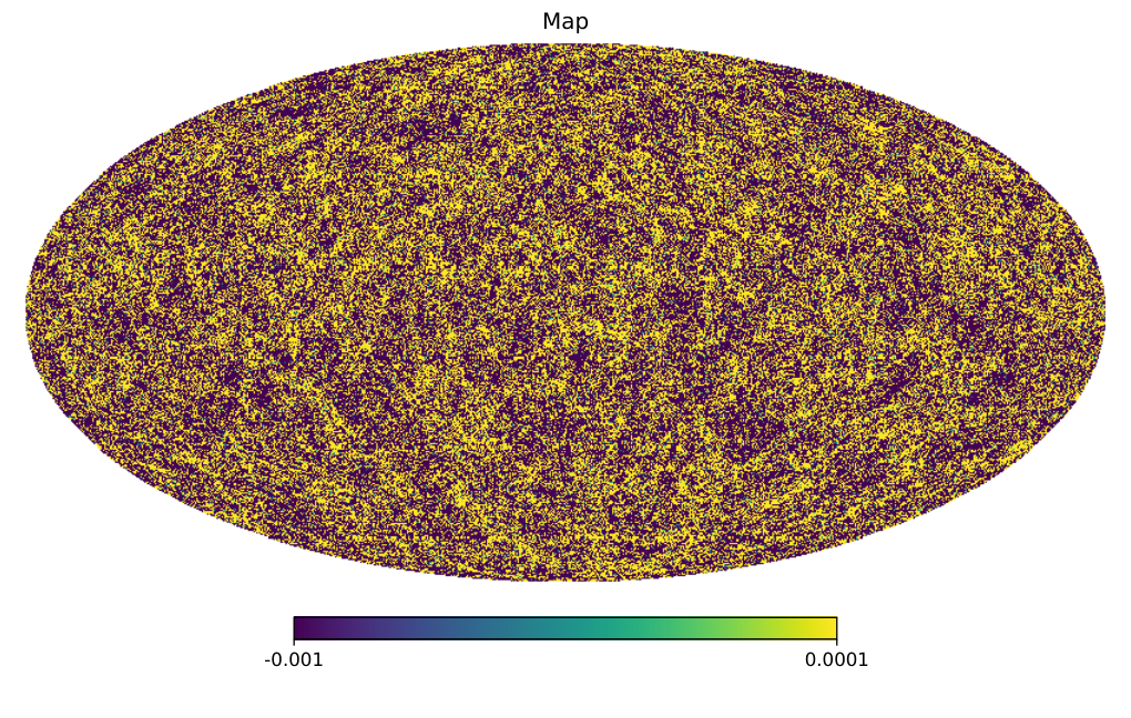
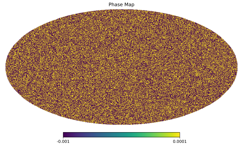
For our study, we have used high resolution maps . These maps were degraded to various lower resolution In Figure 1 we show one such map for the source redshift (left panel) and the corresponding phase map (right panel). We analysed these maps using publicly available software TreeCorr1414 14 https://rmjarvis.github.io/TreeCorr/_build/html/index.html for the computation of two- and three-point correlation functions. The tso-point correlation functions are shown in Figure-2.
LCF for : The line correlation function defined in Eq.(3.8b) is being plotted as a function of In Figure - 3. From left to right we show results for source redshifts , and . We have presented the mean results estimated from ten all-sky maps. No noise was included in our study. Degraded maps with and were respectively used to estimate the correlation function for the range and . The fitting function presented in [43] was used to compute the theoretical predictions. For the sake of completeness we have also shown the two-point correlation function of the maps in Figure - 2 for various redshifts, In this study we will see that at the low source redshift Post-Born correction plays a negligible role, but they play a significant role at higher redshift, e.g. in case of lensing of CMB.
LCF for phase: In Figure - 4 the LCF is being plotted as a function of (in arcmin). The solid lines correspond to the ones defined in Eq.(3.10b) and the dashed-lines correspond to estimates from simulated all-sky weak lensing maps. Panels from left to right correspond to , and respectively. The dashed-lines in each panel correspond to theoretical predictions computed using Born approximation. We have checked that the post-Born corrections do not make any appreciable difference. We have used ten realisations of all-sky maps to compute the numerical estimates. No noise was included. Degraded maps with and were respectively used to estimate the correlation function for the range and . We use for our study. The theoretical results were computed using the fitting function presented in [43].
Skew-spectrum for phase: In addition to the LCF we have also introduced the skew-spectrum estimator, not for , but for the phase maps (denoted as ) defined in Eq.(A.13). For the bispectrum we have used the nonlinear fitting function [43] and for the perturbative calculations we have used the SPT result in Eq.(2.3b). We have presented three redshifts and in Fig.5 in different panels as indicated. The simulation results compare reasonably well against nonlinear predictions. We also see departure at high- which is a result of pixelisation. Our simulation results are derived using which are generated by degrading maps originally created at . For PT results to be valid the maps need to be smoothed. We have also included in our analysis which is relevant for CMB studies. The results are plotted in Fig.5 and for CMB lensing in Fig.7. We found that even with a single all-sky realisation we can estimate the with a very high degree of accuracy. We have included realistic noise though it is expected from our previous study [17] inclusion of noise will not change our findings completely.
The importance of Post-Born (PB) corrections for CMB lensing lensing, was underlined in many recent studies, e.g., Ref.[17]. While such corrections do not make any significant contribution they do play important role for high redshift CMB studies. In Fig.7 we have shown the nonlinear results with and without PB corrections. Inclusion of Post-Born corrections is important to reproduce the simulation results. The maps used were of resolution . Higher-order generalisations of is presented in §B.
Cumulant correlators for phase: The cumulant correlators (CCs) carry equivalent information compared to the skew-spectrum as they can be constructed from skew-spectrum. The theoretical cumulant correlator using Eq.(3.11). The numerical results were computed using the TreeCorr. The results are shown in Fig.6. This alows computation of CCs without broad binning as was the case for LCF. The deviation from theoretical prediction in the low- regime is related to the pixelisation effect. A comparison with the results presented for in Fig.4 confirms very high S/N in . The generalisation to higher-order is straightforward and can by cross-correlating -th power of ,i.e., against its -th power, i.e., .
5 Conclusions and Future Prospects
The primary aim of this paper was to introduce statistics of Fourier phases in the context of weak lensing studies. We have introduced the three-point phase correlation LCF to probe the non-Gaussianity in weak lensing convergence maps used in the study of galaxy clustering . In addition, an associated three-point statistics was also introduced for probing statistics of maps. We have used a set of state-of-the-art all-sky simulations of weak lensing convergence maps to test our theoretical results as a function of source redshift. We have generalised both and to higher-order. Next, we have adopted the cumulant correlator typically used for 3D density field and 2D convergence maps for statistics phases. We showed that available theoretical models can reproduce the numerical results with reasonable accuracy and our results can be used to select the range to retain in order to maintain a given level of theoretical accuracy. While we have focussed on weak lensing convergence, the statistical estimators presented here will be useful in other areas cosmology, e.g., galaxy clustering (in real and redshift space) and in clustering of Lyman- absorbers.
Several extensions are possible on the theoretical front. The Effective Field Theory (EFT) provides a framework to extend the validility domain of the standard perturbation theory (SPT). A formulation of the phase statistics in EFT will improve its domain of validity. It will also be interesting to formulate the phase-statistics directly for shear. Theoretical modelling of bispectrum generated by intrinsic alignment [50] will also be useful. The perturbative regime is not particularly affected by gas physics. Nevertheless, -cut filtering can be included [51] to filter out particularly sensitive modes.
Finally, our study was performed in a rather idealized observational setting to establish a baseline. Realistically complex follow-up studies will be presented in future. In particular a Fisher-based analysis independently and jointly with power spectrum will be presented elsewhere.
References
- [1] Cosmology from Cosmic Shear with DES Science Verification Data, The Dark Energy Survey Collaboration, T Abbott, F. B. Abdalla, S. Allam, et al., 2016, Phys. Rev. D, 94, 022001 [arxiv/1507.0552]
- [2] The WiggleZ Dark Energy Survey: Survey Design and First Data Release, Drinkwater, M. J., R. J. Jurek, C. Blake, et al., 2010, MNRAS, 401, 14 [astro-ph/0911.4246]
- [3] SDSS-III: Massive Spectroscopic Surveys of the Distant Universe, the Milky Way Galaxy, and Extra-Solar Planetary Systems, D. J. Eisenstein, D. H. Weinberg, E. Agol, et al., 2011, AJ, 142, 72 [astro-ph/1101.1529]
- [4] Gravitational Lensing Analysis of the Kilo Degree Survey, K. Kuijken, C. Heymans, H. Hildebrandt, et al., 2015, MNRAS, 454, 3500 [arXiv/1507.00738]
- [5] The Hyper Suprime-Cam SSP Survey: Overview and Survey Design Aihara H. et al., 2018, Publications of the Astronomical Society of Japan, Volume 70, Issue SP1, S4; [arXiv/1704.05858]
- [6] Euclid Definition Study Report, R. Laureijs, J. Amiaux, S. Arduini, et al. 2011, ESA/SRE(2011)12.
- [7] LSST: a complementary probe of dark energy, J . A. Tyson, D. M. Wittman, J. F. Hennawi, D. N Spergel, 2003, Nuclear Physics B Proceedings Supplements, 124, 21 [astro-ph/0209632]
- [8] Planck 2018 results. VI. Cosmological parameters, Planck Collaboration, [arxiv/1807.06209]
- [9] Beyond the Cosmological Standard Model, A. Joyce, B. Jain, J. Khoury, M. Trodden, 2015, Phys. Rep., 568, 1 [astro-ph/1407.0059]
- [10] Modified Gravity and Cosmology, T. Clifton, P. G. Ferreira, A. Padilla, S. Skordis, 2012, Phys. Rep., 513, 1, 1 [astro-ph/1106.2476]
- [11] Massive neutrinos and cosmology, J. Lesgourgues, S. Pastor, 2006, Phys. Rep., 429, 307, [astro-ph/1610.02956] [astro-ph/1507.00738]
- [12] Cosmology with Weak Lensing Surveys D. Munshi, P. Valageas, L. Van Waerbeke, A. Heavens Phys.Rept.462:67-121,2008 [arXiv/0612667]
- [13] Higher order statistics of shear field: a machine learning approach C. Parroni, E. Tollet, V. F. Cardone, R. Maoli, R. Scaramella [astro-ph/1612.02264]
- [14] Weak lensing shear and aperture-mass from linear to non-linear scales D. Munshi, P. Valageas, A. J. Barber MNRAS, 2004, 350, 77 [astro-ph/1612.02264]
- [15] Cylinders out of a top hat: counts-in-cells for projected densities C. Uhlemann 2018, MNRAS, 477, 2772U [arXiv/1711.04767]
- [16] Cosmological constraints with weak lensing peak counts and second-order statistics in a large-field survey A. Peel, C.-A. Lin, F. Lanusse, A. Leonard, J.-L. Starck, M. Kilbinger [arXiv/1612.02264]
- [17] Weak Lensing Skew-Spectrum D. Munshi, T. Namikawa, T. D. Kitching, J. D. McEwen, F. R. Bouchet 2020, MNRAS, 498, 6057 [arXiv/2006.12832]
- [18] Estimating the Integrated Bispectrum from Weak Lensing Maps D. Munshi, J. D. McEwen, T. Kitching, P. Fosalba, R. Teyssier, J. Stadel 2020, MNRAS, 493, 3985 [arXiv/1902.04877]
- [19] New Optimised Estimators for the Primordial Trispectrum D. Munshi, A. Heavens, A. Cooray, J. Smidt, P. Coles, P. Serra 2011, MNRAS, 412, 1993 arXiv/0910.3693
- [20] Morphology of Weak Lensing Convergence Maps D. Munshi, T. Namikawa, J. D. McEwen, T. D. Kitching, F. R. Bouchet [arXiv/2010.05669]
- [21] Matter trispectrum: theoretical modelling and comparison to N-body simulations D. Gualdi, S. Novell, H. Gil-Marín, L. Verde 2021, JCAP, 01, 015 arXiv/2009.02290,
- [22] Persistent homology in cosmic shear: constraining parameters with topological data analysis S. Heydenreich, B. Brück, J. Harnois-Déraps 2021, A&A, 648, 74 arxiv/2007.13724,
- [23] Exact Extreme Value Statistics and the Halo Mass Function I. Harrison, P. Coles MNRAS 418, L20-L24 (2011) arXiv/1108.1358,
- [24] The position-dependent matter density probability distribution function Drew Jamieson, Marilena Loverde 2020, Phys. Rev. D 102, 123546 arxiv/2010.07235,
- [25] An adapted filter function for density split statistics in weak lensing P. Burger, P. Schneider, V. Demchenko, J. Harnois-Deraps, C. Heymans, H. Hildebrandt, S. Unruh 2020, A&A 642, A161 (see also arXiv/2006.10778).
- [26] Response function of the large-scale structure of the universe to the small scale inhomogeneities T. Nishimichi, F. Bernardeau, A. Taruya Physics Letters B, Volume 762, p. 247-252. arXiv/1411.2970
- [27] The Weak Lensing Bispectrum Induced By Gravity D. Munshi, T. Namikawa, T. D. Kitching, J. D. McEwen, R. Takahashi, F. R. Bouchet, A. Taruya, B. Bose 2020, MNRAS, 493, 3985
- [28] Large-Scale Structure of the Universe and Cosmological Perturbation Theory F. Bernardeau, S. Colombi, E. Gaztanaga, R. Scoccimarro Phys.Rept.367:1-248,2002 [arXiv/0112551]
- [29] Phase Correlations and Topological Measures of Large-scale Structure P. Coles Data Analysis in Cosmology”, eds V.J. Martinez, E. Martnez-Gonzalez, M.J. Pons-Borderia and E. Saar, Springer-Verlag Lecture Notes in Physics. astro-ph/0502088,
- [30] Phase Correlations in Non-Gaussian Fields Matsubara T., 2003, ApJ., 591, L79 [astro-ph/0303278]
- [31] Statistics of Fourier Modes in Non-Gaussian Fields Matsubara T., 2007, ApJS, 170, 1, [astro-ph/0610536]
- [32] The distribution function of the phase sum as a signature of phase correlation induced by nonlinear gravitational clustering. Hikage C., Matsubara T., Suto Y., 2004, ApJ, 600, 553 [astro-ph/0308472]
- [33] The Universal Behavior of Phase Correlations in Nonlinear Gravitational Clustering P. Watts, P.Coles, A. Melott The Astrophysical Journal, Volume 589, Number 2 arXiv/1611.01160
- [34] Three-point Phase Correlations: A New Measure of Non-linear Large-scale Structure Wolstenhulme R., Bonvin C., Obreschkow D., 2015, ApJ, 804, 132 [arXiv/1409.3007]
- [35] A Robust Measure of Cosmic Structure beyond the Power-Spectrum: Cosmic Filaments and the Temperature of Dark Matter Obreschkow D., Power C., Bruderer M., Bonvin C., 2013, ApJ, 762 [arXiv/1211.5231]
- [36] Cosmology with Phase Statistics: Parameter Forecasts and Detectability of BAO A. Eggemeier, R. E. Smith 2017, MNRAS, 466, 2496 arXiv/1611.01160
- [37] Cosmological Constraints from Fourier Phase Statistics K. Ali, D. Obreschkow, C. Howlett, C. Bonvin, C. Llinares, F. Oliveira Franco, C. Power arXiv/1806.10276
- [38] Probing redshift-space distortions with phase correlations F. O. Franco, C. Bonvin, D. Obreschkow, K. Ali, J. Byun 2019, Phys. Rev. D, 99, 103530 arXiv/1805.10178
- [39] Constraining the growth rate of structure with phase correlations J. Byun, F. Oliveira Franco, C. Howlett, C. Bonvin, D. Obreschkow 2020, MNRAS, 497, 1765B arXiv/2005.06325
- [40] Fast likelihood-free cosmology with neural density estimators and active learning. J. Alsing, T. Charnock, S. Feeney, B. Wandelt. 2019, MNRAS, 488, 4440. [arXiv/1903.00007]
- [41] Cosmological inference from Bayesian forward modelling of deep galaxy redshift surveys. D. K. Ramanah, G. Lavaux, J. Jasche, B. D. Wand elt. 2019, A&A, 621, A69, [arXiv/1903.10524]
- Berardeau [2004] Studying the morphology of reionisation with the triangle correlation function of phases A. Gorce, and J. R. Pritchard 2019, MNRAS, 489, 1321G [arXiv/1903.11402.]
- [43] Fitting the nonlinear matter bispectrum by the Halofit approach R. Takahashi, T. Nishimichi, T. Namikawa, A. Taruya, I. Kayo, K. Osato, Y. Kobayashi, M. Shirasaki 2020, ApJ, 895, 113T [arXiv/1911.07886]
- [44] Full-sky Gravitational Lensing Simulation for Large-area Galaxy Surveys and Cosmic Microwave Background Experiments, R. Takahashi, T. Hamana, M. Shirasaki, T. Namikawa, T. Nishimichi, K. Osato, K. Shiroyama ApJ, 850, 24, (2017) [arXiv/1706.01472]
- Munshi & Regan [2016] Consistency relations in effective field theory D. Munshi, D. Regan, 2017, JCAP, 06, 042M [arXiv/1705.07866]
- [46] The Skewness of the Aperture Mass Statistic M. Jarvis, G. Bernstein, & B. Jain, 2004, MNRAS, 352, 338 [astro-ph/030739]
- Berardeau [2004] The large-scale Gravitational Bias from the Quasilinear Regime F. Bernardeau 1996, A&A, 312, 11 [astro-ph/9602972]
- [48] Impact of post-Born lensing on the CMB, G. Pratten, A. Lewis 2016, JCAP, 08, 047 [arXiv/1905.1136]
- [49]
HEALPix – a Framework for High Resolution Discretization, and Fast Analysis of Data Distributed on the Sphere
Gorski K. M., Hivon E., Banday A. J., Wandelt B. D., Hansen F. K.,
Reinecke M., Bartelman M., 2005, ApJ, .622, 759 [astro-ph/0409513] - Vlah [2020] An EFT description of galaxy intrinsic alignments Z. Vlah, N. E. Chisari, F. Schmidt 2020, JCAP, 01, 025V [arXiv/1910.08085]
- BNT [2018] Observing Baryonic Acoustic Oscillations in tomographic cosmic shear surveys F. Bernardeau, T. Nishimichi, A. Taruya [arXiv/2004.03201]
- [52] Interferometric Observation of Cosmic Microwave Background Anisotropies M. White1, J. E Carlstrom2, M. Dragovan, W. L Holzapfel2 [astro-ph/9712195]
- [53] An All-Sky Analysis of Polarization in the Microwave Background M. Zaldarriaga, U. Seljak 1997, PRD 55, 1830 [astro-ph/9609170]
- [54] Weak Lensing of the CMB: A Harmonic Approach W. Hu 2000, Phys.Rev. D, 62 (2000) 043007 [astro-ph/0001303]
- Pratten & Munshi [2012] Non-Gaussianity in Large Scale Structure and Minkowski Functionals G. Pratten, D. Munshi, 2012, MNRAS, 423, 4, 3209, [1108.1985]
- Bartolo et al. [2004] N. Bartolo, E. Komatsu, S. Matarrese, A. Riotto, 2004, Phys.Rept., 402, 103 [astro-ph/0406398]
Acknowledgment
DM was supported by a grant from the Leverhulme Trust at MSSL when this work was initiated. RT is spported by MEXT/JSPS KAKENHI Grant Numbers 20H0 5855, 20H0 4723 and 17H0 1131. DM would like to thank Peter Taylor for many useful discussions regarding implementation of the software TreeCorr. We would like to thank Alexander Eggemeier for many useful discussions.
Appendix A All-sky Expressions
Our primary aim in this appendix is to develop all-sky estimators presented in the text of the paper. Following [52, 53, 54] the spherical polar co-ordinate , radial co-ordinate Equivalently in the harmonic domain and denotes the polar angle:
| (A.1) |
The flat-sky and its all-sky harmonic counterpart are related by the following expression:
| (A.2a) | |||
| (A.2b) | |||
The spherical harmonic basis and rhe flat sky basis are related by the following expressions:
| (A.3a) | |||
| (A.3b) | |||
Using the expressions Eq.(A.3b) in Eq.(A.3a) we obtain the flat-sky counterpart of the spherical harmonics:
| (A.4a) | |||
| If we use the following expansion of the plane wave: | |||
| (A.4b) | |||
Next, we consider the case of bispectrum and related estimator:
Here the quantity in parentheses is the well-known Wigner- symbol which enforces the rotational invariance. It is only non-zero for the triplets that satisfy the triangular condition and is even. The reduced bispectrum is useful in directly linking the all-sky bispectrum and its flat-sky counterpart. For the convergence field , is defined through the following expression:
The flat-sky bispectrum is similarly defined through:
| (A.11) |
The flat-sky bispectrum is identical to the reduced bispectrum for high multipole [56]. This can be shown by using the following asymptotic relationship:
| (A.12f) | |||
The skew-spectrum in the flat-sky is given by [55]:
| (A.13a) | |||
Here the functions represent the smoothing window functions and is the cosine of the angle between vector and i.e. , where . The skewness in terms of these expressions is given by:
| (A.14) |
Appendix B Higher-order LCFs
In this section we consider generalisation of the third-order LCFs to higher-order. The family of LCFs can be seen as a natural extension of two-point cumulant correlators often used in the literature. LCFs can be thought of as three-point generalisation of two-point cumulant correlators. The following statistics are relevant for the kappa field as well as the for the phases. In this section we generalise the line-correlation to higher order. The fourth- and fifth-order generalisations are as follows.
| (B.1a) | |||
| We have omitted the numerical prefactor. Equivalently we can generalise Eq.(3.10b) to fourth-order: | |||
| (B.1b) | |||
Here, is the trispectrum for the convergence field and is defined as follows:
| (B.2) |
The extension to higher-order can be done in a straight-forward manner:
| (B.3) |
There are no numerical fitting functions beyond bispectrum. Nevertheless, the possibility of upcoming experiments to detect the higher-order correlation has fuelled development in this area in recent years. Notice that these estimators can be useful in diectly probing galaxy clustering in real [36] as well as in redshift space [38] with suitable modifications.