Humanly Certifying Superhuman Classifiers

Qiongkai Xu Christian Walder Chenchen Xu

Abstract

Estimating the performance of a machine learning system is a longstanding challenge in artificial intelligence research. Today, this challenge is especially relevant given the emergence of systems which appear to increasingly outperform human beings. In some cases, this “superhuman” performance is readily demonstrated; for example by defeating legendary human players in traditional two player games. On the other hand, it can be challenging to evaluate classification models that potentially surpass human performance. Indeed, human annotations are often treated as a ground truth, which implicitly assumes the superiority of the human over any models trained on human annotations. In reality, human annotators can make mistakes and be subjective. Evaluating the performance with respect to a genuine oracle may be more objective and reliable, even when querying the oracle is expensive or impossible. In this paper, we first raise the challenge of evaluating the performance of both humans and models with respect to an oracle which is unobserved. We develop a theory for estimating the accuracy compared to the oracle, using only imperfect human annotations for reference. Our analysis provides a simple recipe for detecting and certifying superhuman performance in this setting, which we believe will assist in understanding the stage of current research on classification. We validate the convergence of the bounds and the assumptions of our theory on carefully designed toy experiments with known oracles. Moreover, we demonstrate the utility of our theory by meta-analyzing large-scale natural language processing tasks, for which an oracle does not exist, and show that under our assumptions a number of models from recent years are with high probability superhuman.

1 Introduction

Artificial Intelligence (AI) agents have begun to outperform humans on remarkably challenging tasks; AlphaGo defeated legendary Go players (Silver et al. 2016; Singh, Okun, and Jackson 2017), and OpenAI’s Dota2 AI has defeated human world champions of the game (Berner et al. 2019). These AI tasks may be evaluated objectively, e.g. using the total score achieved in a game and the victory or defeat against another player. However, for supervised learning tasks such as image classification and sentiment analysis, certifying a machine learning model as superhuman is subjectively tied to human judgments rather than comparing with an oracle. This work focuses on paving a way towards evaluating models with potentially superhuman performance in classification.

Refer to caption — Figure 1: The relationship between a) the oracle accuracy of the annotators, $P(\ell_{i}=\ell_{\star})$ , and b) the agreement between two annotators, $P(\ell_{i}=\ell_{j})$ . $\ell_{i}$ and $\ell_{j}$ are labels given by annotator $i$ and $j$ , $\ell_{\star}$ is the oracle label. In our setting, part a) is unobserved (gray) and part b) is observed (black).

When evaluating the performance of a classification model, we generally rely on the accuracy of the predicted labels with regard to ground truth labels, which we call the oracle accuracy. However, oracle labels may arguably be unobservable. For tasks such as object detection, the predictions are subjective to many factors of the annotators, e.g., their background and physical or mental state. For other tasks, even experts may not be able to summarize an explicit rule for the prediction, such as predicting molecule toxicity and stability. Without observing the oracle labels, human predictions or aggregated human annotations are treated as ground truth (Wang et al. 2018; Lin et al. 2014; Wang et al. 2019) to approximate the oracle. Such approximation mainly suffers from two disadvantages. Firstly, the quality control of human annotation is challenging (Artstein 2017; Lampert, Stumpf, and Gançarski 2016). Secondly, current evaluation paradigms focus on evaluating the performance of models, but not the oracle accuracy of humans — yet we cannot claim that a machine learning model is superhuman without a proper estimation on human performance.

In this paper, we work on the setting that oracle labels are unobserved (see Figure 1). Within this setting, we develop a theory for estimating the oracle accuracy on classification tasks. Our theory includes i) upper bounds for the averaged oracle accuracy of the annotators, ii) lower bounds for the oracle accuracy of the model, and iii) finite sample analysis for both bounds and their margin which represents the model’s outperformance. We propose an algorithm to discover competitive models and to report confidence scores, which formally bound the probability that a given model outperforms the average human annotator. Empirically, we observe that some existing models for sentiment classification and natural language inference (NLI) have already achieved superhuman performance.

2 Related Work

Classification accuracy is a widely used measure of model performance (Han, Pei, and Kamber 2011), although there are other options such as precision, recall, F1-score (Chowdhury 2010; Sasaki et al. 2007), Matthews correlation coefficient (Matthews 1975; Chicco and Jurman 2020), etc.. Accuracy measures the disagreement between the model outputs and some reference labels. A common practice is to collect human labels to treat as the reference. However, we argue that the ideal reference is rather the (unobserved) oracle, as human predictions are imperfect. We focus on measuring the oracle accuracy for both human annotators and machine learning models, and for comparing the two.

A widely accepted approach is to crowd source (Kittur, Chi, and Suh 2008; Mason and Suri 2012) a dataset for testing purposes. The researchers collect a large corpus with each examples labeled by multiple annotators. Then, the aggregated annotations are treated as ground truth labels (Socher et al. 2013; Bowman et al. 2015). This largely reduces the variance of the prediction (Nowak and Rüger 2010; Kruger et al. 2014), however, such aggregated results are still not oracle, and their difference to oracle remains unclear. In our paper, we proves that the accuracy on aggregated human prediction, as ground truth, could be considered as a special case of the lower bound of oracle accuracy for machine learning models. On the other hand, much work considers the reliability of collected data, by providing the agreement scores between annotators (Landis and Koch 1977). Statistical measures for the reliability of inter-annotator agreement (Gwet 2010), such as Cohen’s Kappa (Pontius Jr and Millones 2011) and Fleiss’ Kappa (Fleiss 1971), are normally based on the raw agreement ratio. However, the agreement between annotators does not obviously reflect the oracle accuracy; e.g. identical predictions from two annotators does not mean they are both oracles. In our paper, we prove that observed agreement between all annotators could serve as an upper bound for the average oracle accuracy of those annotators. Overall, we propose a theory for comparing the oracle accuracy of human annotators and machine learning models, by connecting the aforementioned bounds.

The discovery that models can predict better than human experts dates back at least to the seminal and controversial work of Meehl 1954, which compared ad hoc predictions based on subjective and informal information to those based on simple linear models with a (typically small) number of relevant numeric attributes. Subsequent work found that one may even train such a model to mimic the predictions made by the experts (rather than an oracle), and yet still maintain superior out of sample performance (Goldberg 1970). The comparison of human and algorithmic decision making remains an active topic of psychology research (Kahneman, Sibony, and Sunstein 2021).

3 Evaluation Theory

In this section, we present the theory for comparing the oracle accuracy for classification tasks between human annotators and machine learning models.

3.1 Problem Statement

We are given $K$ labels crowd sourced from $K$ human annotators, $\{\ell_{i}\}_{i=1}^{K}$ , along some labels from a model $\ell_{\mathcal{M}}$ . We denote $\ell_{a}^{(n)}$ and $\ell_{\mathcal{M}}^{(n)}$ the label assigned by annotator $a$ and model $\mathcal{M}$ to the $n$ -th data point, for $n=1,2,\dots,N$ . We observe the ratio of matched labels $\mathbb{P}(\ell_{a}=\ell_{b})$ for all of a pairs of annotators $a$ and $b$ . Denote by $\ell_{\mathcal{K}}$ the label of the “average” human annotator which we define as the label obtained by selecting one of the $K$ human annotators uniformly at random. We seek to formally compare the oracle accuracy of the average human, $\mathbb{P}(\ell_{\mathcal{K}}=\ell_{\star})$ , with that of the machine learning model, $\mathbb{P}(\ell_{\mathcal{M}}=\ell_{\star})$ , where $\ell_{\star}$ is the unobserved oracle label. Denote by $\ell_{\mathcal{G}}$ the label obtained by aggregating (say, by majority voting) the $K$ human annotators’ labels. Our work distinguishes between the oracle accuracy $\mathbb{P}(\ell_{\mathcal{M}}=\ell_{\star})$ and the agreement with human annotations $\mathbb{P}(\ell_{\mathcal{M}}=\ell_{\mathcal{G}})$ , although these two concepts have been confounded in many previous applications and benchmarks.

3.2 An Upper Bound for the Average Annotator Performance

The oracle accuracy of the average annotator $\ell_{\mathcal{K}}$ follows the definition of the previous section, and conveniently equals the average of the oracle accuracy of each annotator, i.e.

\mathbb{P}(\ell_{\mathcal{K}}=\ell_{\star})=\frac{1}{K}\sum_{i=1}^{K}\mathbb{P}(\ell_{i}=\ell_{\star}).

(1)

By introducing an assumption, also discussed in Section 4.2, we may bound the above quantity.

Theorem 1 (Average Performance Upper Bound).

Assume annotators are positively correlated, namely $\mathbb{P}(\ell_{i}=\ell_{\star}|\ell_{j}=\ell_{\star})\geq\mathbb{P}(\ell_{i}=\ell_{\star})$ . Then, the upper bound of averaged annotator accuracy with respect to the oracle is

\mathbb{P}(\ell_{\mathcal{K}}=\ell_{\star})\leq\mathcal{U}\triangleq\sqrt{\frac{1}{K^{2}}\sum_{i=1}^{K}\sum_{j=1}^{K}\mathbb{P}(\ell_{i}=\ell_{j})}.

(2)

Proof.

For $i\neq j$ and $i,j\in\{1,\cdots,K\}$ , we have

$\displaystyle\mathbb{P}(\ell_{i}=\ell_{j})=$	$\displaystyle\mathbb{P}(\ell_{i}=\ell_{j}\|\ell_{j}=\ell_{\star})\mathbb{P}(\ell_{j}=\ell_{\star})+$
	$\displaystyle\mathbb{P}(\ell_{i}=\ell_{j}\|\ell_{j}\neq\ell_{\star})\mathbb{P}(\ell_{j}\neq\ell_{\star})$
$\displaystyle\geq$	$\displaystyle\mathbb{P}(\ell_{i}=\ell_{j}\|\ell_{j}=\ell_{\star})\mathbb{P}(\ell_{j}=\ell_{\star})$
$\displaystyle=$	$\displaystyle\mathbb{P}(\ell_{i}=\ell_{\star}\|\ell_{j}=\ell_{\star})\mathbb{P}(\ell_{j}=\ell_{\star})$
$\displaystyle\geq$	$\displaystyle\mathbb{P}(\ell_{i}=\ell_{\star})\mathbb{P}(\ell_{j}=\ell_{\star}).$	(3)

While for $i=j$ , we have $\mathbb{P}(\ell_{i}=\ell_{j})=1$ . Therefore,

\mathbb{P}(\ell_{i}=\ell_{j})\geq\mathbb{P}(\ell_{i}=\ell_{\star})\mathbb{P}(\ell_{j}=\ell_{\star}).

(4)

Then, combining (3) and (4),

$\displaystyle\mathbb{P}(\ell_{\mathcal{K}}=\ell_{\star})^{2}=$	$\displaystyle\frac{1}{K^{2}}\sum_{i=1}^{K}\mathbb{P}(\ell_{i}=\ell_{\star})\sum_{j=1}^{K}\mathbb{P}(\ell_{j}=\ell_{\star})$	(5)
$\displaystyle\leq$	$\displaystyle\frac{1}{K^{2}}\sum_{i=1}^{K}\sum_{j=1}^{K}\mathbb{P}(\ell_{i}=\ell_{j})$	(6)
$\displaystyle\mathbb{P}(\ell_{\mathcal{K}}=\ell_{\star})\leq$	$\displaystyle\sqrt{\frac{1}{K^{2}}\sum_{i=1}^{K}\sum_{j=1}^{K}\mathbb{P}(\ell_{i}=\ell_{j})}.$	(7)

We observe that $\mathbb{P}(\ell_{i}=\ell_{j})$ is overestimated as $1$ when $i=j$ , but that the total overestimation to $\mathcal{U}^{2}$ is less or equal to $1/K$ ( $K$ out of $K^{2}$ terms), and that the influence will reduce and converge to zero as $K\rightarrow\infty$ . To calibrate the overestimation, we introduce an empirically approximated upper bound $\mathcal{U}^{(e)}$ . In contrast, $\mathcal{U}$ in (2) is also noted as theoretical upper bound, $\mathcal{U}^{(t)}$ .

Definition 1.

The empirically approximated upper bound,

\mathcal{U}^{(e)}\triangleq\sqrt{\frac{1}{K(K-1)}\sum_{i=1}^{K}\sum_{\begin{subarray}{c}j=1\\ i\neq j\end{subarray}}^{K}\mathbb{P}(\ell_{i}=\ell_{j})}.

(8)

Lemma 2 (Convergence of $\mathcal{U}^{(e)}$ ).

Assume that $\mathbb{P}(\ell_{i}=\ell_{j})\geq 1/N_{c}$ , where $N_{c}$ is number of classes. The approximated upper bound $\mathcal{U}^{(e)}$ satisfies

\lim_{K\rightarrow+\infty}\mathcal{U}/\mathcal{U}^{(e)}=1.

(9)

Therefore, with large $K$ , $\mathcal{U}^{(e)}$ converges to $\mathcal{U}$ or $\mathcal{U}^{(t)}$ .

We provide a detailed proof of this Lemma in Appendix A. Some empirical evidences for the convergence of the $\mathcal{U}^{(e)}$ to $\mathcal{U}^{(t)}$ are demonstrated in Section 4.2.

3.3 A Lower Bound for Model Performance

For our next result, we introduce another assumption, also discussed in Section 4.2. Given two predicted labels $\ell_{a}$ and $\ell_{b}$ , we assume that $\ell_{b}$ is reasonably predictive even on those instances that $a$ gets wrong, as per

Theorem 3 (Performance Lower Bound).

Assume that for any incorrect label $\ell_{\times}\neq\ell_{\star}$ ,

\mathbb{P}(\ell_{b}=\ell_{\star}|\ell_{a}\neq\ell_{\star})\geq\mathbb{P}(\ell_{b}=\ell_{\times}|\ell_{a}\neq\ell_{\star}).

(10)

Then, the lower bound for the oracle accuracy of $\ell_{b}$ is

\mathcal{L}\triangleq\mathbb{P}(\ell_{a}=\ell_{b})\leq\mathbb{P}(\ell_{b}=\ell_{\star}).

(11)

Proof.

$\displaystyle\mathbb{P}(\ell_{a}=\ell_{b})=$	$\displaystyle\mathbb{P}(\ell_{b}=\ell_{a}\|\ell_{a}\neq\ell_{\star})\mathbb{P}(\ell_{a}\neq\ell_{\star})+$
	$\displaystyle\mathbb{P}(\ell_{b}=\ell_{a}\|\ell_{a}=\ell_{\star})\mathbb{P}(\ell_{a}=\ell_{\star})$
$\displaystyle\leq$	$\displaystyle\mathbb{P}(\ell_{b}=\ell_{\star}\|\ell_{a}\neq\ell_{\star})\mathbb{P}(\ell_{a}\neq\ell_{\star})+$
	$\displaystyle\mathbb{P}(\ell_{b}=\ell_{a}\|\ell_{a}=\ell_{\star})\mathbb{P}(\ell_{a}=\ell_{\star})$
$\displaystyle=$	$\displaystyle\mathbb{P}(\ell_{b}=\ell_{\star}\|\ell_{a}\neq\ell_{\star})\mathbb{P}(\ell_{a}\neq\ell_{\star})+$
	$\displaystyle\mathbb{P}(\ell_{b}=\ell_{\star}\|\ell_{a}=\ell_{\star})\mathbb{P}(\ell_{a}=\ell_{\star})$
$\displaystyle=$	$\displaystyle\mathbb{P}(\ell_{b}=\ell_{\star}).$	(12)

In practice, a more accurate $\ell_{a}$ gives a tighter lower bound for $\ell_{b}$ , and so we employ the aggregated human annotations for the former (letting $\ell_{a}=\ell_{\mathcal{G}}$ ) to calculate the lower bound of the machine learning model (letting $\ell_{b}=\ell_{\mathcal{M}}$ ), as demonstrated in Section 4.2.

Connection to common practice.

Generally, the ground truth of a benchmark corpus is constructed by aggregating multiple human annotations (Wang et al. 2018; Wang et al. 2019). For example, the averaged sentiment score is used in SST (Socher et al. 2013) and majority of votes in SNLI (Bowman et al. 2015). Then, the aggregated annotations are treated as ground truth to calculate accuracy. Under this setting, the accuracy on the (aggregated) human ground truth may be viewed as a special case of our lower bound.

3.4 Finite Sample Analysis

The results above assume that the agreement probabilities are known; we now connect with the finite sample case where those probabilities are estimated empirically. We begin with a standard concentration inequality (see e.g. (Boucheron, Lugosi, and Massart 2013, § 2.6)),

Theorem 4 (Hoeffding’s Inequality).

Let $X_{1},\dots,X_{N}$ be independent random variables with finite variance such that $\mathbb{P}(X_{n}\in[\alpha,\beta])=1$ , for all $1\leq n\leq N$ . Let

\overline{X}\triangleq\frac{1}{N}\sum_{n=1}^{N}X_{n},

then, for any $t>0$ ,

	$\displaystyle\mathbb{P}(\overline{X}-\mathbb{E}[\overline{X}]\geq+t)\leq\exp\left(-\frac{2Nt^{2}}{(\alpha-\beta)^{2}}\right),$
	$\displaystyle\mathbb{P}(\overline{X}-\mathbb{E}[\overline{X}]\leq-t)\leq\exp\left(-\frac{2Nt^{2}}{(\alpha-\beta)^{2}}\right).$		(13)

Combining this with Thereom 1 we obtain the following.

Theorem 5 (Sample Average Performance Upper Bound).

Take the assumptions of Theorem 1, and let

\displaystyle\mathbb{P}^{(N)}(\ell_{i}=\ell_{j})=\frac{1}{N}\sum_{n=1}^{N}\left[\ell^{(n)}_{i}=\ell^{(n)}_{j}\right]

(14)

be the empirical agreement ratio¹¹ 1 Here $[\cdot]$ is the Iverson bracket.. Define

\displaystyle\delta_{u}=\exp(-2Nt_{u}^{2}).

(15)

With probability at least $1-\delta_{u}$ , for any $t_{u}>0$ ,

\displaystyle\mathbb{P}(\ell_{\mathcal{K}}=\ell_{\star})\leq\sqrt{t_{u}+\frac{1}{K^{2}}\sum_{i=1}^{K}\sum_{j=1}^{K}\mathbb{P}^{(N)}(\ell_{i}=\ell_{j})}.

(16)

Proof.

We apply Theorem 4 with

\displaystyle X_{n}=\frac{1}{K^{2}}\sum_{i=1}^{K}\sum_{j=1}^{K}\left[\ell^{(n)}_{i}=\ell^{(n)}_{j}\right],

(17)

obtaining $X_{n}\in[0,1]$ , i.e. $\alpha=0$ , and $\beta=1$ . Let

\displaystyle\mathcal{U}_{N}\triangleq\sqrt{\frac{1}{K^{2}}\sum_{i=1}^{K}\sum_{j=1}^{K}\mathbb{P}^{(N)}(\ell_{i}=\ell_{j})}.

(18)

Our choice (17) of $X_{n}$ implies $\mathcal{U}_{N}^{2}=\overline{X}$ and $\mathcal{U}^{2}=\mathbb{E}[\overline{X}]$ , and so by (4),

\displaystyle\mathbb{P}\left(\sqrt{t_{u}+\mathcal{U}_{N}^{2}}\leq\mathcal{U}\right)\leq\delta_{u}.

(19)

Rewrite (2) as

\displaystyle\mathbb{P}(\ell_{\mathcal{K}}=\ell_{\star})\leq\mathcal{U},

(20)

which implies

\displaystyle\mathbb{P}\left(\sqrt{t_{u}+\mathcal{U}_{N}^{2}}\leq\mathbb{P}(\ell_{\mathcal{K}}=\ell_{\star})\right)\leq\mathbb{P}\left(\sqrt{t_{u}+\mathcal{U}_{N}^{2}}\leq\mathcal{U}\right).

(21)

Combining (19) with (21) gives the result.

Analagously for Theorem 3, we have

Theorem 6 (Sample Performance Lower Bound).

Take the assumptions of Theorem 3 along with (14). Define

\displaystyle\delta_{l}=\exp(-2Nt_{l}^{2}).

(22)

With probability at least $1-\delta_{l}$ , for any $t_{l}>0$ ,

\displaystyle\mathbb{P}^{(N)}(\ell_{a}=\ell_{b})\leq t_{l}+\mathbb{P}(\ell_{b}=\ell_{\star}).

(23)

Proof.

We apply Theorem 4 with

\displaystyle X_{n}=\left[\ell^{(n)}_{a}=\ell^{(n)}_{b}\right],

(24)

obtaining $X_{n}\in[0,1]$ , i.e. $\alpha=0$ , and $\beta=1$ . Let

\displaystyle\mathcal{L}_{N}\triangleq\mathbb{P}^{(N)}(\ell_{a}=\ell_{b}).

(25)

Now (24) implies $\mathcal{L}_{N}=\overline{X}$ and $\mathcal{L}=\mathbb{P}(\ell_{a}=\ell_{b})=\mathbb{E}[\overline{X}]$ ,

\displaystyle\mathbb{P}\left(\mathcal{L}_{N}-t_{l}\geq\mathcal{L}\right)\leq\delta_{l}.

(26)

Recall (11), $\mathbb{P}(\ell_{a}=\ell_{b})\leq\mathbb{P}(\ell_{b}=\ell_{\star})$ , which implies

\displaystyle\mathbb{P}\left(\mathcal{L}_{N}-t_{l}\geq\mathbb{P}(\ell_{b}=\ell_{\star})\right)\leq\mathbb{P}\left(\mathcal{L}_{N}-t_{l}\geq\mathcal{L}\right).

(27)

Combining (26) with (27) gives the result.

3.5 Detecting and Certifying Superhuman Models

We propose a procedure to discover potentially superhuman models based on our theorems.

•

Calculate the upper bound of the average oracle accuracy of human annotators, $\mathcal{U}_{N}$ , with $N$ samples;
•

Calculate the lower bound of the model oracle accuracy $\mathcal{L}_{N}$ using aggregated human annotations as the reference²² 2 We demonstrate that aggregating the predictions by voting and weighted averaging are effective in improving our bounds. We emphasize however that the aggregated predictions need not be perfect, as we do not assume that this aggregation yields an oracle., with $N$ samples;
•

Check whether the finite sample margin $\mathcal{L}_{N}-\mathcal{U}_{N}$ is larger than zero;
•

Give proper estimation of $t_{u}$ and $t_{l}$ and calculate a confidence score of $\mathbb{P}(\mathcal{L}-\mathcal{U}\geq 0)$ .

Generally, larger margin indicates higher confidence of the out-performance. To formally check confidence for the aforementioned margin we provide

Theorem 7 (Confidence of Out-Performance).

Assume an annotator pool with agreement statistic $\mathcal{U}_{N}$ of (18), and an agreement statistic between model and aggregated annotations $\mathcal{L}_{N}$ of (25). If $\mathcal{L}_{N}>\mathcal{U}_{N}$ then for all $\tau\geq 0$ , $t_{u}\geq 0$ and $t_{l}\geq 0$ that satisfy

\mathcal{L}_{N}-t_{l}-\sqrt{t_{u}+\mathcal{U}_{N}^{2}}=\tau,

(28)

with probability at least $1-\delta_{u}-\delta_{l}$ , the model oracle accuracy exceeds that of the average annotator by $\tau$ , i.e.

\displaystyle\mathbb{P}(\ell_{\mathcal{M}}=\ell_{\star})-\mathbb{P}(\ell_{\mathcal{K}}=\ell_{\star})\geq\tau,

(29)

where

	$\displaystyle\delta_{u}$	$\displaystyle=\exp\left(-2Nt_{u}^{2}\right),$		(30)
	$\displaystyle\delta_{l}$	$\displaystyle=\exp\left(-2Nt_{l}^{2}\right).$		(31)

Proof.

Recall Theorem 5 and Theorem 6,

	$\displaystyle\mathbb{P}\left(\sqrt{t_{u}+\mathcal{U}_{N}^{2}}\leq\mathbb{P}(\ell_{\mathcal{K}}=\ell_{\star})\right)$	$\displaystyle\leq\delta_{u}$
	$\displaystyle\mathbb{P}\left(\mathcal{L}_{N}-t_{l}\geq\mathbb{P}(\ell_{\mathcal{M}}=\ell_{\star})\right)$	$\displaystyle\leq\delta_{l}.$

Then, we have

	$\displaystyle\mathbb{P}\left(\mathbb{P}(\ell_{\mathcal{M}}=\ell_{\star})-\mathbb{P}(\ell_{\mathcal{K}}=\ell_{\star})\geq\tau\right)$
$\displaystyle=$	$\displaystyle\mathbb{P}\left(\mathbb{P}(\ell_{\mathcal{M}}=\ell_{\star})-\mathbb{P}(\ell_{\mathcal{K}}=\ell_{\star})\geq\mathcal{L}_{N}-t_{l}-\sqrt{t_{u}+\mathcal{U}_{N}^{2}}\right)$
$\displaystyle\geq$	$\displaystyle\mathbb{P}\left(\mathbb{P}(\ell_{\mathcal{M}}=\ell_{\star})\geq\mathcal{L}_{N}-t_{l}\cap\mathbb{P}(\ell_{\mathcal{K}}=\ell_{\star})\leq\sqrt{t_{u}+\mathcal{U}_{N}^{2}}\right)$
	$\displaystyle=1-\mathbb{P}\left(\mathbb{P}(\ell_{\mathcal{M}}=\ell_{\star})\leq\mathcal{L}_{N}-t_{l}\cup\mathbb{P}(\ell_{\mathcal{K}}=\ell_{\star})\geq\sqrt{t_{u}+\mathcal{U}_{N}^{2}}\right)$
$\displaystyle\geq$	$\displaystyle 1-\mathbb{P}\left(\mathbb{P}(\ell_{\mathcal{M}}=\ell_{\star})\leq\mathcal{L}_{N}-t_{l})\right)-\mathbb{P}\left(\mathbb{P}(\ell_{\mathcal{K}}=\ell_{\star})\geq\sqrt{t_{u}+\mathcal{U}_{N}^{2}}\right)$
$\displaystyle\geq$	$\displaystyle 1-\delta_{l}-\delta_{u}.$	(32)

Confidence Score Estimation.

The above theorem suggests the confidence score

\displaystyle S=1-\delta_{l}-\delta_{u},

(33)

and we need now only choose the free constants $t_{l},t_{u}$ and $\tau$ , which it depends on. Recall (28),

\tau=\left(\mathcal{L}_{N}-t_{l}\right)-\sqrt{t_{u}+\mathcal{U}_{N}^{2}},

(34)

and remove one degree of freedom parameterise in $t_{u}$ as

t_{l}(t_{u},\tau)=\mathcal{L}_{N}-\tau-\sqrt{t_{u}+\mathcal{U}_{N}^{2}}.

(35)

We are interested in $\mathbb{P}(\mathcal{L}-\mathcal{U}\geq 0)$ and so we may set $\tau=0$ . We offer two alternatives for selecting $t_{u}$ and $t_{l}$ .

Algorithm 1 (Heuristic Margin Separation, HMS). We assign half of the margin to $t_{u}$ ,

t_{u}=\frac{\mathcal{L}_{N}-\mathcal{U}_{N}}{2}.

(36)

Then, with $\tau=0$ we calculate the corresponding

t_{l}=\mathcal{L}_{N}-\sqrt{\frac{\mathcal{L}_{N}-\mathcal{U}_{N}}{2}+\mathcal{U}_{N}^{2}},

(37)

and compute the heuristic confidence score $S$ .

Algorithm 2 (Optimal Margin Separation, OMS).
For an locally (in $t_{u}$ ) optimal confidence score, we perform gradient ascent (Lemaréchal 2012) on $S(t_{u})$ , where

\displaystyle S(t_{u})=1-\delta(t_{u})-\delta(t_{l}(t_{u},0)),

(38)

with $t_{u}$ is initialized as $(\mathcal{L}_{N}-\mathcal{U}_{N})/2$ before optimization³³ 3 For all OMS experiments, we set learning rate 1e-4, and iterate 100 times. We will publish our code upon acceptance..

4 Experiments and Discussion

Previously, we introduced a new theory for analyzing the oracle accuracy of set of classifiers using observed agreements between them. In this section, we demonstrate our theory on several classification tasks, to demonstrate the utility of the theory and reliability of the associated assumptions.

4.1 Experimental Setup

We first consider two classification tasks with oracle labels generated by rules. Given the oracle predictions, we are able to empirically validate the assumptions for our theorems and observe the convergence of the bounds. Then, we apply our theory on two real-world classification tasks and demonstrate that some existing state-of-the-art models have potentially achieved better performance than the (averaged) performance of the human annotators.

Classification tasks with oracle rules.

To validate the correctness of our theory, we collect datasets with observable oracle labels. We construct two visual cognitive tasks, Color Classification and Shape Classification, with explicit unambiguous rules to acquire oracle labels, as follows:

•

Color Classification: the oracle selects the most frequently occuring color of the objects in a given image.
•

Shape Classification: the oracle selects the most frequent occurring shape of the objects in a given image.

For both tasks, the size of the objects is ignored. As illustrated in Figure 2, we vary three colors (Red, Blue and Yellow) and five shapes (Triangle, Square, Pentagon, Hexagon and Circle) for the two tasks, respectively.

For each task, we generated 100 images and recruited 10 annotators from the Amazon Mechanical Turk⁴⁴ 4 https://www.mturk.com to label them. Each randomly generated example includes 20 to 40 objects. We enforce that no objects overlap more than 70% with all others, and that there is only one class with the highest count, to ensure uniqueness of the oracle label. The oracle number of the colors and shapes are recorded to generate oracle labels of the examples. More details about annotation interfaces and guidelines are provided in Appendix B.

Real-World Classification Tasks.

We analyze the performance of human annotators and machine learning models on two real-world NLP tasks, namely sentiment classification and natural language inference (NLI). We use the Stanford Sentiment Treebank (SST) (Socher et al. 2013) for sentiment classification. The sentiment labels are mapped into two classes (SST-2)⁵⁵ 5 Samples with overall neutral scores are excluded as in (Tai, Socher, and Manning 2015). or five classes (SST-5), very negative( $[0,0.2]$ ), negative ( $(0.2,0.4]$ ), neutral( $(0.4,0.6]$ ), positive ( $(0.6,0.8]$ ), and very negative ( $(0.8,1.0]$ ). We use the Stanford Natural Language Inference (SNLI) corpus (Bowman et al. 2015) for NLI. All samples are classified by five annotators into three categories, i.e. Contradiction (C), Entailment (E), and Neutral (N). More details of the datasets are reported in Table 1. In the latter part of this section, we only report the estimated upper bounds on test sets, as we intend to compare them with the performance of machine learning models generally evaluated on test sets.

Dataset	#Test	#Class	#Annot.
SST-2 (Socher et al. 2013)	1,821	2	3
SST-5 (Socher et al. 2013)	2,210	5	3
SNLI (Bowman et al. 2015)	10,000	3	5

Table 1: Statistics of SST and SNLI: the number of test samples, number of classes, and the number of annotators.

(a) Color Classification

(b) Shape Classification

Figure 3: Comparison of sample lower bound

\mathcal{L}_{N}

for model oracle accuracy

\mathbb{P}(\ell_{\mathcal{M}}=\ell_{\star})

. Relatively strong and weak models are indicated by

\mathcal{M}^{(s)}

and

\mathcal{M}^{(w)}

. Another comparison of sample theoretical upper bound

\mathcal{U}_{N}^{(t)}

and sample empirical upper bound

\mathcal{U}_{N}^{(e)}

of average oracle accuracy of annotators

\mathbb{P}(\ell_{\mathcal{K}}=\ell_{\star})

Machine Learning Models.

For both of the classification tasks with known oracles, we treat them as detection tasks and train YOLOv3 models (Redmon and Farhadi 2018) for them. The input image resolution is 608 $\times$ 608 and we use the proposed Darknet-53 as the backbone feature extractor. For comparison, we train two models, a strong model and a weak model, on 512 and 128 randomly generated examples, respectively. All models are trained for a maximum of 200 epochs until convergence. During inference, the model detects the objects and we count each type of object to obtain the prediction.

We compare several representative models and their variants for real-world classification tasks, such as Recurrent Neural Networks (Chen, Ling, and Zhu 2018; Zhou et al. 2015), Tree-based Neural Networks (Mou et al. 2016; Tai, Socher, and Manning 2015), and Pre-trained Transformers (Devlin et al. 2019; Radford et al. 2018; Wang et al. 2020; Sun et al. 2020).

4.2 Results and Discussion

We now conduct several experiments to validate the convergence of the bounds and the validity of the assumptions. We then demonstrate the utility of our theory by detecting superhuman models. We organize the discussion into several research questions (RQ).

RQ1: Will the bounds converge given more annotators?

We first analyze the lower bounds. We demonstrate lower bounds for strong models (s) and weak models (w) in Figure 3 in black and blue lines respectively. Generally, i) the lower bounds $\mathcal{L}_{N}$ are always under the oracle accuracy of corresponding models; ii) the lower bounds grow and tend to get closer to the bounded scores given more aggregated annotators. Then, we analyze the upper bounds. We illustrate theoretical upper bound $\mathcal{U}_{N}^{(t)}$ and empirically approximated upper bound $\mathcal{U}_{N}^{(e)}$ , in comparison with average oracle accuracy of annotators $\mathbb{P}(\ell_{\mathcal{K}}=\ell_{\star})$ , in Figure 3. We observe that i) both upper bounds give higher estimation than the average oracle accuracy of annotators; ii) the margin between $\mathcal{U}_{N}^{(t)}$ and $\mathcal{U}_{N}^{(e)}$ reduce, given more annotators incorporated; iii) $\mathcal{U}_{N}^{(e)}$ generally provides a tighter bound than $\mathcal{U}_{N}^{(t)}$ , and we will use $\mathcal{U}_{N}^{(e)}$ as $\mathcal{U}_{N}$ to calculate confidence score in later discussion.

RQ2: Are the assumptions of our theorems valid?

We verify the key assumptions for the upper bound of Theorem 1 and the lower bound of Theorem 3 by computing the relevant quantities in Table 2. The two assumptions hold in our experiments, although we can only perform this analysis on the tasks with known oracle labels. For the assumptions required for our lower bound, our experiment is more conservative than the assumption, as we sum over all incorrect labels (see column 2 of Table 2.b). Despite the stricter setting, our assumption still holds on both experiments.

(a) Theorem 1 assumes $\mathbb{P}(\ell_{i}=\ell_{\star}\|\ell_{j}=\ell_{\star})\geq\mathbb{P}(\ell_{i}=\ell_{\star})$ , $i\neq j$
Task	$\mathbb{P}(\ell_{i}=\ell_{\star}\|\ell_{j}=\ell_{\star})$	$\mathbb{P}(\ell_{i}=\ell_{\star})$
Color	0.850	0.836
Shape	0.586	0.542
Task $b$	$\mathbb{P}(\ell_{b}=\ell_{\star}\|\ell_{a}\neq\ell_{\star})$	$\sum_{\ell_{\times}\neq\ell_{\star}}\mathbb{P}(\ell_{b}=\ell_{\times}\|\ell_{a}\neq\ell_{\star})$
Color $\mathcal{M}^{(w)}$	1.000	0.000
Color $\mathcal{M}^{(s)}$	1.000	0.000
Shape $\mathcal{M}^{(w)}$	0.579	0.421
Shape $\mathcal{M}^{(s)}$	0.895	0.105
(b) Theorem 3 assumes $\mathbb{P}(\ell_{b}=\ell_{\star}\|\ell_{a}\neq\ell_{\star})\geq\mathbb{P}(\ell_{b}=\ell_{\times}\|\ell_{a}\neq\ell_{\star})$

Table 2: Validating our assumptions for both upper bound Theorem 1 and lower bound Theorem 3 on Color and Shape.

Disclaimer: while the assumptions appear reasonable, we recommend where possible to obtain a small set of oracle labels to validate the assumptions in future research.

	SST 5-Class		SST 2-Class		SNLI 3-Class
B	Classifier	Score	Classifier	Score	Classifier	Score
$\mathcal{U}_{N}^{(t)}$	Avg. Human	0.790 ^‡	Avg. Human	0.960 ^‡	Avg. Human	0.904 ^‡
$\mathcal{U}_{N}^{(e)}$	Avg. Human	0.660 ^†	Avg. Human	0.939 ^†	Avg. Human	0.879 ^†
	CNN-LSTM (Zhou et al. 2015)	0.492	CNN-LSTM (Zhou et al. 2015)	0.878	BiLSTM (Chen, Ling, and Zhu 2018)	0.855
$\mathcal{L}_{N}$	Constituency Tree-LSTM (Tai, Socher, and Manning 2015)	0.510	Constituency Tree-LSTM (Tai, Socher, and Manning 2015)	0.880	Tree-CNN (Mou et al. 2016)	0.821
	BERT-large (Devlin et al. 2019)	0.555	BERT-large (Devlin et al. 2019)	0.949^†	LM-Pretrained Transformer (Radford et al. 2018)	0.899^†
	RoBERTa+Self-Explaining (Sun et al. 2020)	0.591	StructBERT (Wang et al. 2020)	0.971^‡	SemBERT (Zhang et al. 2020)	0.919^‡

Table 3: The sample theoretical upper bounds and sample empirically approximated upper bounds,

\mathcal{U}_{N}^{(t)}

and

\mathcal{U}_{N}^{(e)}

, of the average oracle accuracy of the human annotators, and the sample lower bounds

\mathcal{L}_{N}

of some representative models on the SST and SNLI tasks. Those models with

\mathcal{L}_{N}

higher than

\mathcal{U}_{N}^{(e}

or even

\mathcal{U}_{N}^{(t)}

are highlighted with

\dagger

\ddagger

RQ3: How to identify a ‘powerful’, or even superhuman, classification model?

We first compare the $\mathcal{L}_{N}$ with $\mathcal{U}_{N}$ in our toy experiments, in Figure 3. Overall, it is more likely to observe superhuman performance given more annotators. We observe that $\mathcal{L}_{N}^{(s)}$ outperforms both $\mathcal{U}_{N}^{(e)}$ and $\mathcal{U}_{N}^{(t)}$ , given more than 4 and 6 annotators for color classification and shape classification, respectively. When the model is marginally outperforming human, see weak model for color classification, we may not observe a clear superhuman performance margin, $\mathcal{L}_{N}^{(s)}$ and $\mathcal{U}_{N}^{(e)}$ are very close given more than 7 annotators.

For real-world classification tasks, we i) calculate the average annotator upper bounds given multiple annotators’ labels and ii) collect model lower bounds reported in previous literature. Some results on SST and SNLI are reported in Table 3. We observe that pre-trained language models provide significant performance improvement on those tasks. Our theory manages to identify some of these models that potentially exceed the average human annotator performance, by comparing $\mathcal{U}^{(e)}_{N}$ or the even more restrictive $\mathcal{U}^{(t)}_{N}$ .

RQ4: How confident are the certifications?

We calculate our confidence score for the identified outperforming models via $\mathcal{U_{N}}$ , $\mathcal{L_{N}}$ , $N$ , and using HMS and OMS, as reported in Table 4. Generally, the confidence scores for SNLI models are higher than those of SST-2 because the former has test set is more than five times larger, while more recent and advanced models achieve higher confidence scores as they have larger margin of $\mathcal{L}_{N}-\mathcal{U}_{N}$ .

Model	Task	S(HMS)	S(OMS)
(Devlin et al. 2019)	SST-2	$<0$	$<0$
(Wang et al. 2020)	SST-2	0.4730	0.6208
(Radford et al. 2018)	SNLI	0.8482	0.9267
(Zhang et al. 2020)	SNLI	0.9997	0.9999

Table 4: Confidence score

S

for the certificated models that outperform human annotators in SST-2 and SNLI.

5 Conclusions

In this paper, we built a theory towards estimating the oracle accuracy of classifiers. Our theory covers i) the upper bounds for the average performance of human annotators, ii) lower bounds for machine learning models, and iii) confidence scores which formally capture the degree of certainty to which we may assert that a model outperforms human annotators. Our theory provides formal guarantees even within the highly practically relevant realistic setting of a finite data sample and no access to an oracle to serve as the ground truth. Our experiments on synthetic classification tasks validate the plausibility of the assumptions on which our theorems are built. Finally, our meta analysis of existing progress succeeded in identifying some existing state-of-the-art models have already achieved superhuman performance compared to the average human annotator.

Broader Impact

Our approach can identify classification models that outperform typical humans in terms of classification accuracy. Such conclusions influence the understanding of the current stage of research on classification, and therefore potentially impact the strategies and policies of human-computer collaboration and interaction. The questions we may help to answer include the following: When should we prefer a model’s diagnosis over that of a medical professional? In courts of law, should we leave sentencing to an algorithm rather than a Judge? These questions and many more like them are too important to ignore. Given recent progress in machine learning we believe the work is overdue.

Yet we caution that estimating a model’s oracle accuracy in this way is not free. Our approach requires the results from multiple annotators and preferably also the number of annotators should be higher than the number of possible classes in the target classification task. Another potential challenge in applying our analysis is that some of our assumptions may not hold under some specific tasks or settings. We recommend those who apply our theory where possible to collect a small amount of ‘oracle’ annotations, to validate the assumptions in this paper.

References

Artstein (2017) Artstein, R. 2017. Inter-annotator agreement. In Handbook of linguistic annotation, 297–313. Springer.
Berner et al. (2019) Berner, C.; Brockman, G.; Chan, B.; Cheung, V.; Debiak, P.; Dennison, C.; Farhi, D.; Fischer, Q.; Hashme, S.; Hesse, C.; et al. 2019. Dota 2 with large scale deep reinforcement learning. arXiv preprint arXiv:1912.06680.
Boucheron, Lugosi, and Massart (2013) Boucheron, S.; Lugosi, G.; and Massart, P. 2013. Concentration Inequalities: A Nonasymptotic Theory of Independence. OUP Oxford. ISBN 9780191655500.
Bowman et al. (2015) Bowman, S.; Angeli, G.; Potts, C.; and Manning, C. D. 2015. A large annotated corpus for learning natural language inference. In Proceedings of the 2015 Conference on Empirical Methods in Natural Language Processing, 632–642.
Chen, Ling, and Zhu (2018) Chen, Q.; Ling, Z.-H.; and Zhu, X. 2018. Enhancing Sentence Embedding with Generalized Pooling. In Proceedings of the 27th International Conference on Computational Linguistics, 1815–1826.
Chicco and Jurman (2020) Chicco, D.; and Jurman, G. 2020. The advantages of the Matthews correlation coefficient (MCC) over F1 score and accuracy in binary classification evaluation. BMC genomics, 21(1): 1–13.
Chowdhury (2010) Chowdhury, G. G. 2010. Introduction to modern information retrieval. Facet publishing.
Devlin et al. (2019) Devlin, J.; Chang, M.-W.; Lee, K.; and Toutanova, K. 2019. BERT: Pre-training of Deep Bidirectional Transformers for Language Understanding. In Proceedings of the 2019 Conference of the North American Chapter of the Association for Computational Linguistics: Human Language Technologies, Volume 1 (Long and Short Papers), 4171–4186.
Fleiss (1971) Fleiss, J. L. 1971. Measuring nominal scale agreement among many raters. Psychological bulletin, 76(5): 378.
Goldberg (1970) Goldberg, L. 1970. Man versus model of man: A rationale, plus some evidence, for a method of improving on clinical inferences. 422–432.
Gwet (2010) Gwet, K. L. 2010. Handbook of inter-rater reliability Advanced Analytics. LLC, Gaithersburg, MD.
Han, Pei, and Kamber (2011) Han, J.; Pei, J.; and Kamber, M. 2011. Data mining: concepts and techniques. Elsevier.
Kahneman, Sibony, and Sunstein (2021) Kahneman, D.; Sibony, O.; and Sunstein, C. 2021. Noise: a Flaw in Human Judgment. William Collins.
Kittur, Chi, and Suh (2008) Kittur, A.; Chi, E. H.; and Suh, B. 2008. Crowdsourcing user studies with Mechanical Turk. In Proceedings of the SIGCHI conference on human factors in computing systems, 453–456.
Kruger et al. (2014) Kruger, J.; Endriss, U.; Fernandez, R.; and Qing, C. 2014. Axiomatic analysis of aggregation methods for collective annotation. In Proceedings of the 2014 international conference on Autonomous agents and multi-agent systems, 1185–1192.
Lampert, Stumpf, and Gançarski (2016) Lampert, T. A.; Stumpf, A.; and Gançarski, P. 2016. An empirical study into annotator agreement, ground truth estimation, and algorithm evaluation. IEEE Transactions on Image Processing, 25(6): 2557–2572.
Landis and Koch (1977) Landis, J. R.; and Koch, G. G. 1977. The measurement of observer agreement for categorical data. biometrics, 159–174.
Lemaréchal (2012) Lemaréchal, C. 2012. Cauchy and the gradient method. Doc Math Extra, 251(254): 10.
Lin et al. (2014) Lin, T.-Y.; Maire, M.; Belongie, S.; Hays, J.; Perona, P.; Ramanan, D.; Dollár, P.; and Zitnick, C. L. 2014. Microsoft coco: Common objects in context. In European conference on computer vision, 740–755. Springer.
Mason and Suri (2012) Mason, W.; and Suri, S. 2012. Conducting behavioral research on Amazon’s Mechanical Turk. Behavior research methods, 44(1): 1–23.
Matthews (1975) Matthews, B. W. 1975. Comparison of the predicted and observed secondary structure of T4 phage lysozyme. Biochimica et Biophysica Acta (BBA)-Protein Structure, 405(2): 442–451.
Meehl (1954) Meehl, P. E. 1954. Clinical versus statistical prediction: A theoretical analysis and a review of the evidence Minneapolis: University of Minnesota Press. [Reprinted with new Preface. 136–141.
Mou et al. (2016) Mou, L.; Men, R.; Li, G.; Xu, Y.; Zhang, L.; Yan, R.; and Jin, Z. 2016. Natural Language Inference by Tree-Based Convolution and Heuristic Matching. In Proceedings of the 54th Annual Meeting of the Association for Computational Linguistics (Volume 2: Short Papers), 130–136.
Nowak and Rüger (2010) Nowak, S.; and Rüger, S. 2010. How reliable are annotations via crowdsourcing: a study about inter-annotator agreement for multi-label image annotation. In Proceedings of the international conference on Multimedia information retrieval, 557–566.
Pontius Jr and Millones (2011) Pontius Jr, R. G.; and Millones, M. 2011. Death to Kappa: birth of quantity disagreement and allocation disagreement for accuracy assessment. International Journal of Remote Sensing, 32(15): 4407–4429.
Radford et al. (2018) Radford, A.; Narasimhan, K.; Salimans, T.; and Sutskever, I. 2018. Improving Language Understanding by Generative Pre-Training.
Redmon and Farhadi (2018) Redmon, J.; and Farhadi, A. 2018. Yolov3: An incremental improvement. arXiv preprint arXiv:1804.02767.
Sasaki et al. (2007) Sasaki, Y.; et al. 2007. The truth of the f-measure. 2007. URL: https://www. cs. odu. edu/˜ mukka/cs795sum09dm/Lecturenotes/Day3/F-measure-YS-26Oct07. pdf [accessed 2021-05-26].
Silver et al. (2016) Silver, D.; Huang, A.; Maddison, C. J.; Guez, A.; Sifre, L.; Van Den Driessche, G.; Schrittwieser, J.; Antonoglou, I.; Panneershelvam, V.; Lanctot, M.; et al. 2016. Mastering the game of Go with deep neural networks and tree search. nature, 529(7587): 484–489.
Singh, Okun, and Jackson (2017) Singh, S.; Okun, A.; and Jackson, A. 2017. Learning to play Go from scratch. Nature, 550(7676): 336–337.
Socher et al. (2013) Socher, R.; Perelygin, A.; Wu, J.; Chuang, J.; Manning, C. D.; Ng, A. Y.; and Potts, C. 2013. Recursive deep models for semantic compositionality over a sentiment treebank. In Proceedings of the 2013 conference on empirical methods in natural language processing, 1631–1642.
Sun et al. (2020) Sun, Z.; Fan, C.; Han, Q.; Sun, X.; Meng, Y.; Wu, F.; and Li, J. 2020. Self-Explaining Structures Improve NLP Models.
Tai, Socher, and Manning (2015) Tai, K. S.; Socher, R.; and Manning, C. D. 2015. Improved Semantic Representations From Tree-Structured Long Short-Term Memory Networks. In Proceedings of the 53rd Annual Meeting of the Association for Computational Linguistics and the 7th International Joint Conference on Natural Language Processing (Volume 1: Long Papers), 1556–1566.
Wang et al. (2019) Wang, A.; Pruksachatkun, Y.; Nangia, N.; Singh, A.; Michael, J.; Hill, F.; Levy, O.; and Bowman, S. R. 2019. SuperGLUE: a stickier benchmark for general-purpose language understanding systems. In Proceedings of the 33rd International Conference on Neural Information Processing Systems, 3266–3280.
Wang et al. (2018) Wang, A.; Singh, A.; Michael, J.; Hill, F.; Levy, O.; and Bowman, S. R. 2018. GLUE: A Multi-Task Benchmark and Analysis Platform for Natural Language Understanding. In International Conference on Learning Representations.
Wang et al. (2020) Wang, W.; Bi, B.; Yan, M.; Wu, C.; Xia, J.; Bao, Z.; Peng, L.; and Si, L. 2020. StructBERT: Incorporating Language Structures into Pre-training for Deep Language Understanding. In International Conference on Learning Representations.
Zhang et al. (2020) Zhang, Z.; Wu, Y.; Zhao, H.; Li, Z.; Zhang, S.; Zhou, X.; and Zhou, X. 2020. Semantics-aware BERT for language understanding. In Proceedings of the AAAI Conference on Artificial Intelligence, volume 34, 9628–9635.
Zhou et al. (2015) Zhou, C.; Sun, C.; Liu, Z.; and Lau, F. 2015. A C-LSTM neural network for text classification. arXiv preprint arXiv:1511.08630.

Appendix A Proof Details

Proof of Lemma 2

$\displaystyle\frac{\mathcal{U}}{\mathcal{U}^{(e)}}=$	$\displaystyle\sqrt{\frac{K-1}{K}\frac{\sum_{i=1}^{K}\sum_{j=1}^{K}\mathbb{P}(\ell_{i}=\ell_{j})}{\sum_{i=1}^{K}\sum_{\begin{subarray}{c}j=1\\ i\neq j\end{subarray}}^{K}\mathbb{P}(\ell_{i}=\ell_{j})}}$
$\displaystyle=$	$\displaystyle\sqrt{\frac{K-1}{K}}\sqrt{1+\frac{\sum_{i=1}^{K}\mathbb{P}(\ell_{i}=\ell_{i})}{\sum_{i=1}^{K}\sum_{\begin{subarray}{c}j=1\\ i\neq j\end{subarray}}^{K}\mathbb{P}(\ell_{i}=\ell_{j})}}$
$\displaystyle=$	$\displaystyle\sqrt{\frac{K-1}{K}}\sqrt{1+\frac{K}{\sum_{i=1}^{K}\sum_{\begin{subarray}{c}j=1\\ i\neq j\end{subarray}}^{K}\mathbb{P}(\ell_{i}=\ell_{j})}}$	(39)

For the first factor in (39),

\lim_{K\rightarrow+\infty}\sqrt{\frac{K-1}{K}}=1.

(40)

For the second factor in (39), as both annotators address the same task, the annotator agreement should be better than guessing uniformly at random, i.e. $\mathbb{P}(\ell_{i}=\ell_{j})\geq 1/N_{c}$ , where $N_{c}$ is the number of classes. Then, we have

0\leq\frac{K}{\sum_{i=1}^{K}\sum_{\begin{subarray}{c}j=1\\ i\neq j\end{subarray}}^{K}\mathbb{P}(\ell_{i}=\ell_{j})}\leq\frac{N_{c}}{K-1}.

As $\lim_{K\rightarrow+\infty}\frac{N_{c}}{K-1}=0$ ,

\lim_{K\rightarrow+\infty}\sqrt{1+\frac{K}{\sum_{i=1}^{K}\sum_{\begin{subarray}{c}j=1\\ i\neq j\end{subarray}}^{K}\mathbb{P}(\ell_{i}=\ell_{j})}}=1.

(41)

Combining (40) and (41), we have

\lim_{K\rightarrow+\infty}\frac{\mathcal{U}}{\mathcal{U}^{(e)}}=1.

(42)

Appendix B Details for Annotation

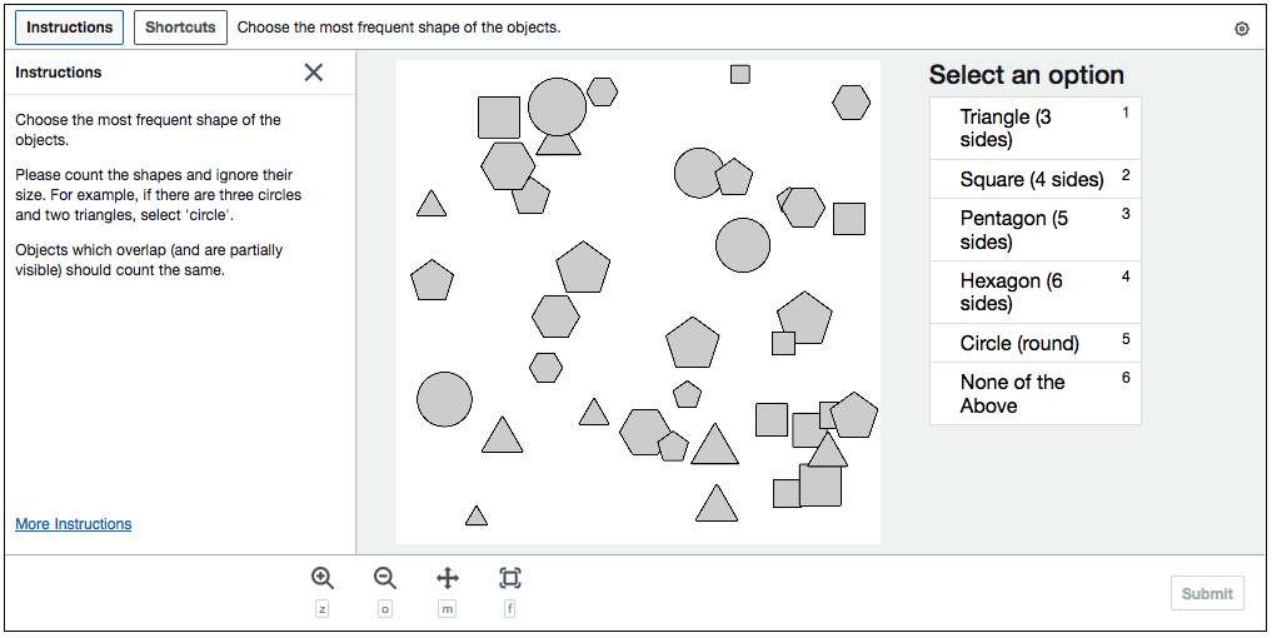
We crowd source the annotations via the Amazon Mechanical Turk. The annotation interfaces with instructions for color classification and shape classification are illustrated in Figure 4. Each example is annotated by $K=10$ different annotators. For quality control, we i) offer our tasks only to experienced annotators with 100 or more approved HITs; ii) automatically reject answers from annotators who have selected ‘None of the above’.

Humanly Certifying Superhuman Classifiers

Abstract

1 Introduction

2 Related Work

3 Evaluation Theory

3.1 Problem Statement

3.2 An Upper Bound for the Average Annotator Performance

Theorem 1 (Average Performance Upper Bound).

Proof.

Definition 1.

Lemma 2 (Convergence of 𝒰(e)\mathcal{U}^{(e)}).

3.3 A Lower Bound for Model Performance

Theorem 3 (Performance Lower Bound).

Proof.

Connection to common practice.

3.4 Finite Sample Analysis

Theorem 4 (Hoeffding’s Inequality).

Theorem 5 (Sample Average Performance Upper Bound).

Proof.

Theorem 6 (Sample Performance Lower Bound).

Proof.

3.5 Detecting and Certifying Superhuman Models

Theorem 7 (Confidence of Out-Performance).

Proof.

Confidence Score Estimation.

4 Experiments and Discussion

4.1 Experimental Setup

Classification tasks with oracle rules.

Real-World Classification Tasks.

Machine Learning Models.

4.2 Results and Discussion

RQ1: Will the bounds converge given more annotators?

RQ2: Are the assumptions of our theorems valid?

RQ3: How to identify a ‘powerful’, or even superhuman, classification model?

RQ4: How confident are the certifications?

5 Conclusions

Broader Impact

References

Appendix A Proof Details

Proof of Lemma 2

Appendix B Details for Annotation

Lemma 2 (Convergence of $\mathcal{U}^{(e)}$ ).