Confining and chiral properties of QCD in extremely strong magnetic fields
Abstract
We investigate, by numerical lattice simulations, the static quark-antiquark potential, the flux tube properties and the chiral condensate for QCD with physical quark masses in the presence of strong magnetic fields, going up to GeV2, with continuum extrapolated results. The string tension for quark-antiquark separations longitudinal to the magnetic field is suppressed by one order of magnitude at the largest explored magnetic field with respect to its value at zero magnetic background, but is still non-vanishing; in the transverse direction, instead, the string tension is enhanced but seems to reach a saturation at around 50 % of its value at . The flux tube shows a consistent suppression/enhancement of the overall amplitude, with mild modifications of its profile. Finally, we observe magnetic catalysis in the whole range of explored fields with a behavior compatible with a lowest Landau level approximation, in particular with a linear dependence of the chiral condensate on which is in agreement, within errors, with that already observed for GeV2.
pacs
12.38.Aw, 11.15.Ha,12.38.GcI Introduction
In the recent past, various analytic and numerical studies have uncovered a plenty of interesting new phenomena regarding the non-perturbative properties of strong interactions in the presence of a magnetic background field Yamamoto:2021oys; Ding:2020hxw; Hofmann:2020ism; Cao:2019azh; lecnotmag; anisotropic; chernodub; musak; elze1; elze2; mueller; galilo; simonov2; KojoSu1; KojoSu2; watson; andersen; ozaki; kamikado; mueller2; demusa; DEN; Ilgenfritz:2012fw; reg2; EB; kovacs; Ilgenfritz:2013ara; DElia:2018xwo; catalreview; fukuhida; Bornyakov:2013eya; Chao:2013qpa; Fraga:2013ova; Yu:2014sla; Ferreira:2014kpa; Farias:2014eca; Ruggieri:2014bqa; strongmag0; strongmag1; tusso; Bonati:2017uvz; DElia:2015eey; Bali:2011qj; Bali:2012cd; rhomass1; rhomass2; rhomass3; rhomass4; simonov; Kojo:2021gvm; Hattori:2019ijy; Machado1; Machado2; Alford; Filip; Dudal:2014jfa; Cho:2014loa; Bonati:2015dka; Suzuki:2016kcs; Finazzo:2016mhm; Yoshida:2016xgm; Suzuki:2016fof; Iwasaki:2018pby; Iwasaki:2018czv; Khan:2021syq; Iwasaki:2021nrz; Zhou:2020ssi. Some of these phenomena might be of direct phenomenological relevance for heavy ion experiments hi1; hi2; hi3; hi4; tuchin or astrophysics magnetars; vacha; grarub, some of them are more speculative but nevertheless interesting. Among these phenomena, a direct impact on the QCD vacuum properties, in particular those regarding the pure gauge sector, is particularly striking, since gluons are not electrically charged, and might be the signal of a stronger impact of the magnetic field on the QCD phase structure.
In Refs. strongmag0; strongmag1, a direct effect on the static quark-antiquark potential has been unveiled, consisting mostly of a suppression of the string tension for quark-antiquark separations parallel to the magnetic background, and of an enhancement for transverse separations; such findings have been confirmed in Ref. tusso by a direct investigation of the color flux tube properties and can be interpreted within various model computations anisotropic; galilo; Giataganas:2012zy; Ferrer:2014qka; Rougemont:2014efa; Chernodub:2014uua; Miransky:2015ava; Simonov:2015yka; Endrodi:2015oba; Schafer:2015wja; Dudal:2016joz; Hasan:2017fmf; Giataganas:2018uuw; Andreichikov:2018wrc.
In particular, the conclusions of Ref. strongmag1 pointed to the possible presence of a critical magnetic field GeV2, above which the longitudinal string tension would vanish, resulting in a different and yet unknown phase of strongly interacting matter. Such conclusions, however, were not based on direct simulations performed at such large values of the magnetic background, but just on the extrapolation of results obtained in a smaller magnetic field range.
Given the new and interesting predicted phenomena, a direct investigation is of utmost importance. As we will better explain in the following Sections, the main difficulty in studying large magnetic backgrounds by lattice simulations is that the ultraviolet (UV) cut-off must be tuned correspondingly in order to keep discretization errors under control and allow for a reliable continuum extrapolation. In this study we will investigate QCD with physical quark masses and lattice spacings down to fm, which is around half the finest spacing explored in Ref. strongmag1, with a similar discretization based on stout-improved staggered fermions. That will allow us to obtain continuum extrapolated results for up to GeV2, which is enough to confirm or update the prediction of Ref. strongmag1. In addition to that, we will consider the chiral properties of the theory, in particular the chiral condensate, to investigate if magnetic catalysis is still at work.
The paper is organized as follows. In Section II we provide more details regarding the adopted discretization of QCD in the presence of a magnetic background, as well as about the lattice observable used to extract the potential and the chromoelectric field between the static quark-antiquark pair. In Section III, after some preliminary details regarding our numerical simulations, we illustrate our results for the chiral condensate, the static potential and the color flux tube. Finally, in Section IV, we summarize our conclusions.
II Numerical Methods
We consider QCD in the presence of a uniform and constant, external magnetic field, discretized in terms of the tree-level improved Symanzik action weisz; curci for the gauge sector, and of rooted staggered fermions with stout improvement kogut-susskind; morning for the fermionic sector. The resulting partition function is
| (1) |
where is the group invariant integration measure on the link variables, the flavor index,
| (2) |
is the lattice gauge action, and
| (3) |
is the discretized Dirac operator. There, labels lattice sites and the direction, while is the inverse gauge coupling and the lattice spacing. The s are the real parts of the trace of the links products along the and rectangular closed path, respectively. The are the staggered quark phases, and is the two times stout smeared link (with isotropic smearing parameter ).
An external electromagnetic (e.m.) field is added by minimal substitution in the covariant derivative
| (4) |
where are the gluon fields, the generators, the abelian four-potential, and and are respectively the bare strong coupling constant and the quark electric charge. We consider for simplicity a uniform magnetic field in the direction, a possible gauge choice is then:
| (5) |
That can be discretized on a periodic toroidal lattice in terms of link variables as follows
| (6) |
where is the lattice extension along the direction (in lattice units) and the right hand side (RHS) condition is needed to guarantee smoothness of the magnetic field across the periodic boundaries wiese; review; according to Eq. (5), all other abelian links are set to . Notice that, consistently with the required zero net magnetic flux across the lattice torus, the above links lead to a constant magnetic field but for a single plaquette, which is pierced by an additional Dirac string: invisibility of that string leads to a quantization condition for the magnetic field thooft; bound3; wiese; review
| (7) |
considering that the smallest quark charge is . The external field is finally added to the discretization of QCD decribed above by the following substitution in the Dirac operator in Eq. (3):
| (8) |
Notice that in this approach the e.m. field is treated as purely external, neglecting the back-reaction of quarks on it, and meaning in practice that no additional integration over the gauge links is introduced in the partition function.
Bare masses and gauge coupling values have been set in order to move on a line of constant physics, determined in Refs. tcwup1; befjkkrs; physline3 to reproduce experimental results for hadronic observables at zero temperature in the continuum limit. The introduction of the external field leads to additional, -dependent discretization errors. In particular, one should consider that the magnetic field acts in practice through the gauge invariant phase factors that dynamical quarks pick going through closed loops on the lattice: the smallest non-trivial such loop is the plaquette in the plane, for which the phase factor is
| (9) |
Systematic errors in the discretization of the magnetic field are under control if such phase is much smaller than : for the up quark, which has the largest electric charge , the condition reads:
| (10) |
a useful way to visualize such systematics is to think that the existence of this minimal phase pickable by dynamical up quarks is like saying that we are approximating a circle by a regular polygon with sides. All that also sets a natural UV cut-off for the largest magnetic fields which are explorable for a given lattice spacing, which is roughly . We have spent a few additional words on these aspects, since this will be essential to properly discuss discretization effects in our investigation, where extremely strong magnetic fields (one order of magnitude larger than the standard QCD scale) are considered.
II.1 Observables
To get the static potential of a -pair, similarly to Refs. strongmag0; strongmag1, we studied the Wilson loop and its dependence on the Euclidean time , exploiting the relation
| (11) |
which holds for large enough . In particular, from previous equation one can derive
| (12) |
so that the potential at fixed can be obtained by fitting to a constant the in the RHS of Eq. (12) as a function of , at least in a suitable stability range.
The color flux tube instead was studied, following Ref. tusso, by means of the connected correlator-probe scheme Cea:2017ocq; DiGiacomo; DiGiacomo:1990hc; Cea:1992vx; Cea:2012qw; Cea:2014uja; Baker:2019: the observable computed to derive chromoelectric field in-between the static quark-antiquark pair is in this case:
| (13) |
where is the open Wilson loop, is the open plaquette in the -plane and the Schwinger path linking the former two operators, while is the distance between the plaquette and Wilson loop plane, i.e. the distance from the quark-antiquark axis. One can easily prove that, in the naive continuum limit,
| (14) |
which can be considered as a probe of the color field strength induced by the presence of the quark-antiquark pair, i.e., with some abuse of notation, as .

The connected correlator is pictorially described in Fig. 1: is attached to the square Wilson loop in the midpoint of its temporal extent, it reaches half the distance between the quark-antiquark pair and then it moves lattice spacings in one of the directions orthogonal to the plane of the Wilson loop: in this way the flux tube profile is determined at the midpoint of the static color source. In this case, as in Ref. tusso, the investigation has been limited to squared Wilson loops.
It is important to note that the presence of the background magnetic field along breaks the spatial octahedral symmetry, leaving a symmetry on the -plane. In the evaluation of the static potential by means of the Wilson loop, this condition implies that loops in the -direction are not equivalent to those extending in - and -directions, which on the other hand are equivalent to each other: that naturally leads to distinguish between a static potential measured longitudinally (L) to the magnetic field, or transverse (T) to it. Actually, one can consider also generic angles between the magnetic field direction and the quark-antiquark axis: this is best done by considering magnetic fields with a generic orientation relative to the lattice axes. This kind of more general analysis has been performed in Ref. strongmag1, showing however that most of the angular dependence of the static potential can be accounted for by the lowest harmonic. That means that the relevant information is contained in the L and T-potentials, which are therefore the only cases considered in the present investigation.
The study of the correlator is a bit more involved, due to its three-dimensional shape. Apart from the T- or L-cases characterizing the orientation of the quark-antiquark separation relative to the magnetic field, in the T-case one can further distinguish whether the flux tube profile is studied in the direction parallel or orthogonal to : the analysis of Ref. tusso shows that some minor anisotropies emerge also in this case, i.e. the flux tube itself loses its axial symmetry. Therefore, as for the flux tube profile, we will consider three different cases: L, TL and TT. We denote by the direction of the quark-antiquark axis, so that the possible geometries can be mapped into these three equivalence classes according to Table 1.
| class | ||
|---|---|---|
| L | ||
| TT | ||
| TL | ||
A residual symmetry is preserved but, anyway, it has not been exploited in this work.
For the evaluation of both observables in order to reduce the UV noise, we applied one step of HYP smearing Hasenfratz:2001hp for temporal links, with the following choice of parameters: (as for the HYP2-action defined in Ref. Della Morte:2005yc). Moreover, we performed several steps of (spatial) APE smearing Albanese:1987ds on the spatial links, so that the -times smeared link reads
| (15) |
where , is the sum of the spatial staples around the link , denotes the projection on the gauge group and the choices for match those of previous works: for the string tension as in strongmag1 and for the QCD flux tube as in tusso.
III Numerical Results
| lattice size | ||||
|---|---|---|---|---|
| 0.114 | 3.787 | 0.0457 | 0,41,93 | |
| 0.086 | 3.918 | 0.0343 | 0,41,93 | |
| 0.057 | 4.140 | 0.0224 | 0,41,93 |
Our results are based on simulations corresponding to three different values of (0, 4 and 9 GeV2) and three different lattice spacings in each case ( and 0.114 fm) in order to allow for a continuum extrapolation; simulations at zero magnetic field have been performed mostly for renormalization purposes. The spatial lattice size has been kept fixed in most cases to fm, with an Euclidean temporal extent twice as large. A summary of all simulation points is reported in Table 2. Monte-Carlo sampling of gauge configurations has been performed based on a Rational Hybrid Monte-Carlo (RHMC) algorithm running on GPUs openacc1; openacc2. For each simulation we performed RHMC steps, taking measures every unit trajectories. The statistical analysis has been based in most cases on a binned bootstrap analysis.

In our analysis we will assume the lattice spacing being independent of . This is a reasonable assumption as long as the magnetic field is much smaller than the UV cutoff, hence it is expected to lead to sensible results at least when continuum extrapolations are considered. As a matter of fact, the assumption has been explicitly checked only for smaller values of the magnetic field Bali:2011qj; however our analysis of the chiral condensate, leading to results in agreement with theoretical expectations, will further support the hypothesis.
III.1 Magnetic catalysis at extremely large magnetic fields
Before focusing on the confining aspects of the theory, let us discuss its chiral properties, for which predictions are well established. In particular one expects, at least for , the magnetic catalysis phenomenon, with an enhancement of chiral symmetry breaking induced by the magnetic background field and detectable as an increase of the chiral condensate.
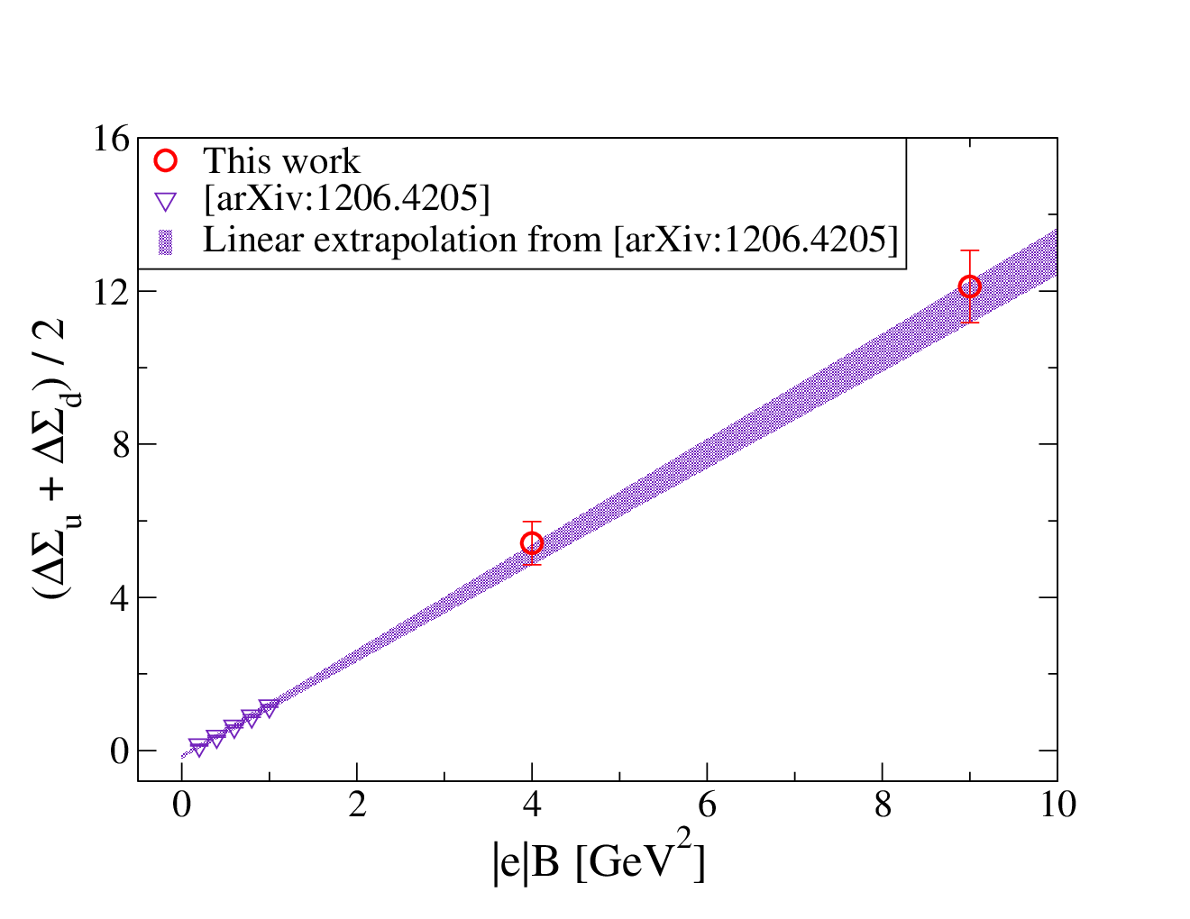
In order to compare with previous results in the literature, we will consider the change of the light quark condensate due to the magnetic field, renormalized as in Ref. Bali:2012cd:
| (16) |
with , where is determined as usual in terms of the volume normalized trace of the inverse fermion matrix (computed by noisy estimators), MeV is the pion mass and MeV is the pion decay constant in the chiral limit.
The average quantity is displayed in Fig. 2 for the two explored values of as a function of the squared lattice spacing , together with a continuum extrapolation obtained assuming corrections. It is interesting to notice that continuum corrections are significantly larger for GeV2: that can be easily understood in terms of what discussed above regarding the -dependent discretization errors (see Eq. (10) and comments thereafter). For GeV2, corresponding to , these kind of discretization errors, at the three different lattice spacings, can be put in analogy with those that one has by approximating a circle by a regular polygon with respectively (from coarsest to finest) 7, 12, 28 sides, which is reasonable right from the beginning; for GeV2 instead, corresponding to , the approximation starts with a triangle (which is far from good) and ends with a dodecagon (which is reasonable). These considerations make it clearer why, having in mind to perform a reliable continuum extrapolation, it is not reasonable to consider larger values of , unless smaller lattice spacings are computationally affordable.
In Fig. 3 continuum extrapolated results are compared to the analogous ones obtained, for GeV2, in Ref. Bali:2012cd. The large field behavior of the magnetic catalysis phenomenon can be thoretically predicted in terms of a lowest Landau level (LLL) approximation. The higher energy levels increase proportionally to , thus they become practically irrelevant to the dynamics of the system. The LLL is instead independent of , while its degeneracy linearly increases with it: that leads to predict a linear behavior in the density of near-zero modes, hence in the chiral condensate by the Banks-Casher relation. This linear behavior is nicely reproduced in Fig. 3: in particular, in the figure we display the result of a linear fit to data from Ref. Bali:2012cd which, when extrapolated to the large magnetic fields explored in this study, is perfectly compatible with our results within errors.
Notice that the lattice spacing enters with a fourth power in fixing the renormalization group invariant quantity in Eq. (16): hence, the nice consistency with data from Ref. Bali:2012cd and with the LLL prediction supports the assumption that the lattice spacing is indeed independent of .
III.2 Static quark-antiquark potential
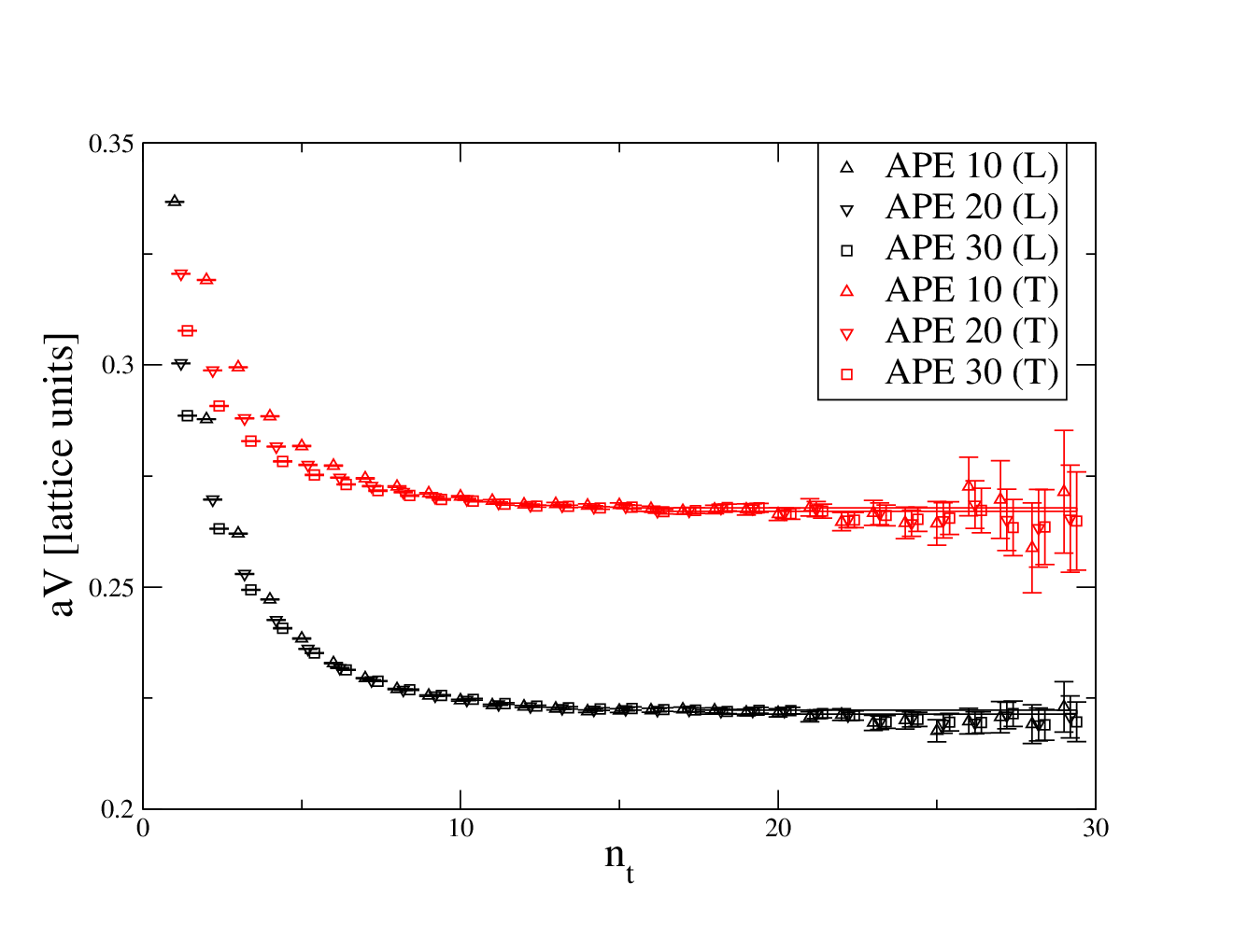
The static quark-antiquark potential has been derived as described above, by looking for a plateau, as a function of the temporal extent , for the logarithm of Wilson loop ratios reported in Eq. (12). An example is showed in Fig. 4, where we report data obtained for both the trasverse and longitudinal direction at GeV2 and for the finest lattice spacing. The two bands show our final determination of the potential for the two cases and have been obtained considering Wilson loops after 30 spatial APE smearing steps, however we report in the figure also data obtained after 10 and 20 smearing steps, which are practically indistinguishable. A similar stability under APE smearing is observed for all explored values of , lattice spacing and quark-antiquark separation .

In Fig. 5 we show the final determination of the static potential obtained for the finest lattice spacing and all the explored values of . The anisotropy which is present when is clearly evident, even if in the transverse direction it shows a non-monotonic behavior with , with a tendency for a slight decrease of the slope when going from 4 to 9 GeV2, at least for this value of the lattice spacing.
As a preliminary analysis, we have considered results for the potential at and compared them with previous results in the literature, in order to check consistency. In particular, in Fig. 6 we compare results obtained for the string tension in this work with those obtained in Ref. strongmag1 using the same lattice discretization but different lattice spacings. The two sets of results are perfectly compatible with each other and a combined continuum extrapolation assuming corrections returns a continuum value MeV with (the point on the coarsest lattice being discarded), which is perfectly compatible with phenomenological predictions and lattice determinations for Aoki:2016frl. We would like to stress the importance of this consistency check: since the physical spatial lattice sizes adopted in this work and in Ref. strongmag1 are, for computational reasons, quite different ( fm vs fm), the agreement we find shows that, at least for what concerns the static quark-antiquark potential, finite size effects are not significant.

Next, in order to assess to the fate of the static potential anisotropy in the explored range of magnetic fields, we consider, as in Ref. strongmag1, the dimensionless ratios , which are reported in Fig. 7 as a function of for both magnetic fields and for both the longitudinal and the transverse directions, together with continuum extrapolations assuming corrections. Regarding the string tension in the longitudinal direction, we confirm the findings of Ref. strongmag1: it is a consistently decreasing function of , both for at finite lattice spacing and in the continuum limit; however, contrary to the hypothesis put forward in Ref. strongmag1, we find a non-zero string tension, within two standard deviations, even at the largest explored value of . Regarding the transverse direction, instead, we can appreciate from Fig. 7 that, at least for finite lattice spacing, the trend for an increasing string tension observed in Ref. strongmag1 seems inverted. However, when considering continuum extrapolations, one realizes that actually reaches a saturation at large .


Such results are better appreciable in Fig. 8, where the continuum extrapolated values for in the T- and L-directions obtained in this study are compared with the continuum extrapolation of Ref. strongmag1, which is plotted only in the relevant range of where simulations of Ref. strongmag1 were performed. Present results are not inconsistent with those of Ref. strongmag1, however they clarify the perspective for the large- limit of the string tension. In the trasverse direction, the string tension seems to reach a saturation at a value which is around 50 % larger than the zero field value. In the longitudinal direction the string tension keeps decreasing as a function of , but is still significantly different from zero for GeV2, contrary to what the continuum extrapolation of Ref. strongmag1 could have suggested: the large field behavior is difficult to predict precisely, it could be either an exponential-like decreasing behavior for which the string tension never vanishes, or a more straight decrease where finally vanishing at some critical value for GeV2. Such possibility should be further explored by future studies, capable of approaching even smaller values of the lattice spacing, which has been the main constraint limiting our simulations to GeV2 in order to access properly extrapolated continuum results.
III.3 Color flux tubes

The analysis of color flux tubes is expected, in general, to confirm results obtained by the analysis of the static quark-antiquark potential: this is indeed the outcome of Ref. tusso, showing that the main effect of the magnetic field is an overall suppression/enhancement of the flux tube in the L/T directions, with a slight modification of its profile, which however can be still nicely described by models inspired to dual superconductivity of the QCD vacuum.
We measured the longitudinal component of the chromo-electric field (directed along the quark-antiquark axis) since previous studies showed that it is by far the dominant one (see Baker:2019 and references therein). We denote by the direction where the color charges lay, so that the longitudinal chromo-electric field is given by
| (17) |
where is the separation distance between the quark-antiquark pair and is the transverse distance at which the field is probed (see Fig. 1).
The use of smearing techniques introduces a non trivial dependence on the amount of smearing adopted. On the other hand, the analysis of Ref. tusso showed that ratios of observables with and without the magnetic field, such as , are insensitive to the number of smearing steps. We verified that this feature holds true for the extreme magnetic fields investigated in this study, as illustrated in Fig. 9, where we show the ratios of the chromo-electric fields obtained at fm for each magnetic field choice and inequivalent class of Table 1. We display the flux tubes at but, anyway, the independence is observed for each value of the transverse distance. Since we are interested in similar ratios of observables, we unambigously decided to fix for the analysis carried out for each lattice spacing and value of , so that the dependence on will be dropped in the following.
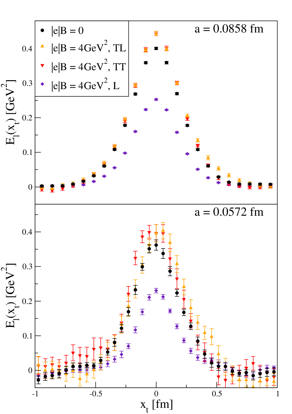
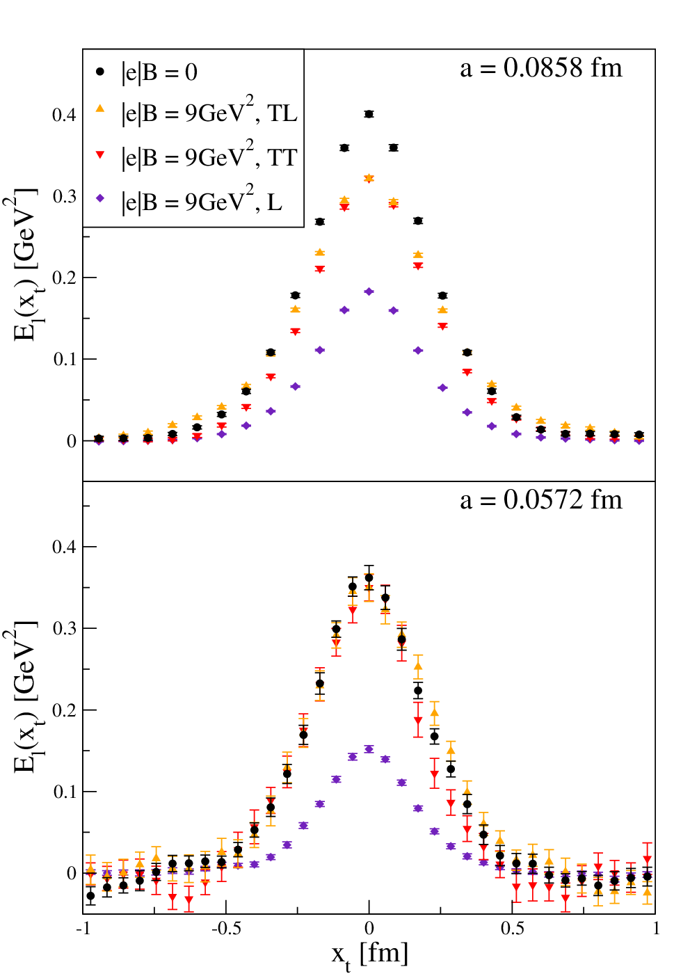
In Fig. 10 and Fig. 11 we show some results for the flux tube extracted from simulations performed at lattice spacings fm, using Wilson loops of spatial size fm. The influence of the background field on the color flux tube is compatible with the findings of the previous section: strong anisotropies are induced depending on the magnitude and orientation of the external field. In detail, in the L case the flux tube monotonically decreases as the magnetic field grows; in transverse cases (TT-TL), the chromo-electric field is enhanced at GeV2 while a non-trivial dependence on the lattice spacing is exhibited for GeV2: the flux tube is suppressed by the magnetic field at fm and compatible with the case at fm. We stress that this trend is consistent with the scaling dependence on observed for the string tension extracted in transverse cases at GeV2 (see Fig. 7).
In Fig. 12 we show the ratio for each magnetic field value and geometry class at fm. Results clearly point out the loss of the cylindrical symmetry in transverse configurations, since the TT an TL cases are not equivalent. Furthermore, both at and GeV2 the ratio is a decreasing function of in the L case, meaning that the color flux tube gets squeezed by the background field. This behaviour had already been outlined at weaker fields in Ref. tusso, whose results are displayed together with our findings in Fig. 13.


The comparison points out two effects:
- •
the squeezing phenomenon seems to reach a saturation for large fields, since the decreasing dependence on is quite similar for GeV2;
- •
flux tubes are monotonically suppressed by the increasing background magnetic field. On the other hand, a qualitative weakening of the dependece on can be noticed, in agreement with the behaviour of the string tension outlined in Fig. 8 and discussions thereafter.
Despite the observed deformations, the functional dependence of the flux tube profile does not seem to change significantly. We employ a parametrization inspired by the form of magnetic fields inside vortices in type II superconductors to fit the data for the longitudinal chromo-electric field. In particular, we follow the parametrization proposed in Clem, where an expression for the magnetic flux tube which solves the Ginzburg-Landau equations is obtained by a variational model for the normalized order parameter of an isolated vortex. This expression, often called Clem ansatz, reads
| (18) |
where are the modified Bessel functions of the second kind of order while and are fit parameters. Previous studies showed that the flux tube profile is well described by the Clem function, also in the presence of an external field tusso. Remarkably, we find that the expression in Eq. (18) is a suitable model even at the large magnetic fields explored in this work. As an example, in Fig. 14 we show the chromo-electric fields obtained at the finest lattice spacing in L configurations together with the best fit functions. We checked that the fit works reasonably well for all the choices of magnetic field, geometry class and lattice spacing.

Flux tubes can be used to compute a more significant parameter: the linear energy density . Since the transverse components of the chromo-electric field are negligible, the energy density just reads
| (19) |
The integration is performed over the section orthogonal to the quark-antiquark pair axis, requiring to explicitly know the angular dependence of the color flux tubes. However, the chromo-electric field possess a cylindrical symmetry over the plane when is directed along the charges (L configurations), so that it is independent of the azimuthal angle. In this case, the integration procedure can be pursued based on data extracted along just one direction on the plane. Furthermore, a numerical integration is not needed: assuming the expression in Eq. (18), then the known integrals of the modified Bessel functions can be exploited (see, e.g., Eq. (5.52.1) and Eq. (5.54.2) in Ref.integrali), leading to
| (20) |
so that the linear energy density can be expressed in terms of best fit parameters. This allows to avoid problems regarding the numerical integration instability and the systematic uncertainties which would arise due to the sharp peaks of the flux tube profile.

So, we show in Fig. 15 the ratio extracted from L configurations for both the values of the background field and each lattice spacing, together with the continuum extrapolations performed assuming corrections.
In a classical picture, the energy density per unit length is strictly related to the string tension, since the latter is nothing but the slope of the linear term in the potential. A direct comparison is not possible due to the strong dependence of on the smearing procedure. However, this issue is overcome by taking into account the ratio , where the dependence on is expected to disappear. Actually, the fact that the ratio is independent of the smearing procedure, as seen in Fig. 9, does not imply a priori that ratios of fit parameters (and so ) are independent too. Nevertheless, this independence is numerically observed in the energy density for all the values of . The comparison is hence possible and it is performed in Fig. 16, where the continuum limit of the ratio is shown together with the ratio of the string tension extracted in the longitudinal case: results are in nice agreement, whithin errors.

IV Conclusions
The motivation for the present work lies in Refs. strongmag0; strongmag1; tusso, and in particular Ref. strongmag1, where a prediction was made for a possible vanishing of the string tension for quark-antiquark separations in the direction longitudinal to a magnetic background field and for field values GeV2, based however on the extrapolation of results obtained from simulations at smaller field values. Which kind of new QCD phase could emerge, if any, where the string tension vanishes in just one direction, is an intriguing question which deserves an answer.
In order to make progress in this direction, in this study we have pushed the range of magnetic background fields explorable by lattice simulations, with a control over the continuum extrapolation, by considering a set of three different lattice spacings, going down to fm, and a discretization of QCD similar to that of Refs. strongmag0; strongmag1; tusso, i.e. based on stout improved rooted staggered fermions. In this way, we have been able to reach GeV2.
The main result is that, contrary to the expectations of Ref. strongmag1, the string tension in the longitudinal direction is clearly non-vanishing for GeV2 and still at two standard deviations from zero even at GeV2, where however it is suppressed by one order of magnitude with respect to its value at zero magnetic background. On the other hand, the enhancement of the string tension, as a function of , in the transverse direction seems to reach a saturation at around 50 % of the string tension value at .
The analysis of the color flux tube shows a consistent suppression/enhancement of its overall amplitude, with mild modifications of its profile, consistent with those already observed in Ref. tusso. In particular, one observes a mild squeezing of the flux tube of quark-antiquark separations parallel to the magnetic field, and a loss of cylindrical symmetry for transverse separations. Notwithstanding such deformations, the flux tube profile is still describable by models inspired to dual superconductivity of the QCD vacuum in all the explored cases.
Finally, the analysis of the chiral condensate shows a persistence of magnetic catalysis in the whole range of explored fields, with a behavior compatible with a lowest Landau level approximation, in particular with a linear dependence of the chiral condensate on which is in agreement, within errors, with that already observed for GeV2 in Ref. Bali:2012cd.
To summarize, present results postpone to even larger magnetic fields the possibile emergence of a new phase of strong interactions, characterized by the vanishing of the string tension for quark-antiquark separation parallel to the magnetic field, and by other possible associated new phenomena which have not been observed so far. The critical field could be not far from where we are now, since the longitudinal string tension is at just two standard deviations from zero at the largest explored field, however a careful investigation will require simulations on finer lattices: in the future we plan to put further efforts along this direction. A different direction is to investigate QCD at finite temperature for the same lattice spacings and magnetic background fields explored in the present study, since that could give indications about the phase structure from a different perspective: work is in progress along this line wip.
Acknowledgements.
We thank M. Cardinali for collaboration in the early stages of this study. Numerical simulations have been performed on the MARCONI and MARCONI100 machines at CINECA, based on the Project IscrB_STROMAG and on the agreement between INFN and CINECA (under projects INF20_npqcd, INF21_npqcd). F.S. is supported by the Italian Ministry of University and Research (MUR) under grant PRIN20172LNEEZ and by INFN under GRANT73/CALAT.References
- (1) D. Kharzeev, K. Landsteiner, A. Schmitt and H. -U. Yee, Lect. Notes Phys. 871, 1 (2013).
- (2) V. A. Miransky and I. A. Shovkovy, Phys. Rev. D 66, 045006 (2002);
- (3) I. A. Shovkovy, Lect. Notes Phys. 871, 13 (2013) [arXiv:1207.5081 [hep-ph]].
- (4) A. Yamamoto, Eur. Phys. J. A 57 (2021) no.6, 211 [arXiv:2103.00237 [hep-lat]].
- (5) M. M. Musakhanov and F. C. Khanna, hep-ph/9605232.
- (6) H. T. Elze and J. Rafelski, In *Sandansky 1998, Frontier tests of QED and physics of the vacuum* 425-439 [hep-ph/9806389].
- (7) H. T. Elze, B. Muller and J. Rafelski, hep-ph/9811372.
- (8) M. Asakawa, A. Majumder and B. Muller, Phys. Rev. C 81, 064912 (2010). [arXiv:1003.2436 [hep-ph]].
- (9) B. V. Galilo and S. N. Nedelko, Phys. Rev. D 84, 094017 (2011). [arXiv:1107.4737 [hep-ph]].
- (10) M. N. Chernodub, arXiv:1001.0570 [hep-ph].
- (11) M. A. Andreichikov, V. D. Orlovsky and Y. .A. Simonov, Phys. Rev. Lett. 110, no. 16, 162002 (2013) [arXiv:1211.6568 [hep-ph]].
- (12) T. Kojo and N. Su, Phys. Lett. B 720, 192 (2013) [arXiv:1211.7318 [hep-ph]].
- (13) T. Kojo and N. Su, Phys. Lett. B 726, 839 (2013) [arXiv:1305.4510 [hep-ph]].
- (14) P. Watson and H. Reinhardt, Phys. Rev. D 89, 045008 (2014) [arXiv:1310.6050 [hep-ph]].
- (15) J. O. Andersen, W. R. Naylor and A. Tranberg, arXiv:1311.2093 [hep-ph].
- (16) S. Ozaki, Phys. Rev. D 89, 054022 (2014) [arXiv:1311.3137 [hep-ph]].
- (17) K. Kamikado and T. Kanazawa, JHEP 1403, 009 (2014) [arXiv:1312.3124 [hep-ph]].
- (18) N. Mueller, J. A. Bonnet and C. S. Fischer, arXiv:1401.1647 [hep-ph].
- (19) M. D’Elia, S. Mukherjee and F. Sanfilippo, Phys. Rev. D 82, 051501 (2010) [arXiv:1005.5365 [hep-lat]].
- (20) M. D’Elia and F. Negro, Phys. Rev. D 83, 114028 (2011) [arXiv:1103.2080 [hep-lat]].
- (21) G. S. Bali, F. Bruckmann, G. Endrodi, Z. Fodor, S. D. Katz, S. Krieg, A. Schafer and K. K. Szabo, JHEP 1202, 044 (2012) [arXiv:1111.4956 [hep-lat]].
- (22) G. S. Bali, F. Bruckmann, G. Endrodi, Z. Fodor, S. D. Katz and A. Schafer, Phys. Rev. D 86, 071502 (2012) [arXiv:1206.4205 [hep-lat]]
- (23) E. -M. Ilgenfritz, M. Kalinowski, M. Muller-Preussker, B. Petersson and A. Schreiber, Phys. Rev. D 85, 114504 (2012) [arXiv:1203.3360 [hep-lat]].
- (24) G. S. Bali, F. Bruckmann, G. Endrodi, F. Gruber and A. Schaefer, JHEP 1304, 130 (2013) [arXiv:1303.1328 [hep-lat]].
- (25) M. D’Elia, M. Mariti and F. Negro, Phys. Rev. Lett. 110, 082002 (2013) [arXiv:1209.0722 [hep-lat]].
- (26) F. Bruckmann, G. Endrodi and T. G. Kovacs, JHEP 1304, 112 (2013) [arXiv:1303.3972 [hep-lat]].
- (27) E. -M. Ilgenfritz, M. Muller-Preussker, B. Petersson and A. Schreiber, arXiv:1310.7876 [hep-lat].
- (28) M. D’Elia, F. Manigrasso, F. Negro and F. Sanfilippo, Phys. Rev. D 98, no.5, 054509 (2018) [arXiv:1808.07008 [hep-lat]].
- (29) H. T. Ding, S. T. Li, A. Tomiya, X. D. Wang and Y. Zhang, Phys. Rev. D 104 (2021) no.1, 014505 [arXiv:2008.00493 [hep-lat]].
- (30) C. P. Hofmann, Phys. Rev. D 102 (2020) no.9, 094010 [arXiv:2006.07717 [hep-ph]].
- (31) G. Cao and T. Kojo, [arXiv:1911.09898 [hep-ph]].
- (32) K. Fukushima and Y. Hidaka, Phys. Rev. Lett. 110, 031601 (2013) [arXiv:1209.1319 [hep-ph]].
- (33) V. G. Bornyakov, P. V. Buividovich, N. Cundy, O. A. Kochetkov and A. Schäfer, arXiv:1312.5628 [hep-lat].
- (34) J. Chao, P. Chu and M. Huang, Phys. Rev. D 88, 054009 (2013) [arXiv:1305.1100 [hep-ph]].
- (35) E. S. Fraga, B. W. Mintz and J. Schaffner-Bielich, Phys. Lett. B 731, 154 (2014) [arXiv:1311.3964 [hep-ph]].
- (36) L. Yu, H. Liu and M. Huang, arXiv:1404.6969 [hep-ph].
- (37) M. Ferreira, P. Costa, O. Lourenço, T. Frederico and C. Providencia, arXiv:1404.5577 [hep-ph].
- (38) R. L. S. Farias, K. P. Gomes, G. I. Krein and M. B. Pinto, arXiv:1404.3931 [hep-ph].
- (39) M. Ruggieri, L. Oliva, P. Castorina, R. Gatto and V. Greco, arXiv:1402.0737 [hep-ph].
- (40) C. Bonati, M. D’Elia, M. Mariti, M. Mesiti, F. Negro and F. Sanfilippo, Phys. Rev. D 89, 114502 (2014) [arXiv:1403.6094 [hep-lat]]
- (41) C. Bonati, M. D’Elia, M. Mariti, M. Mesiti, F. Negro, A. Rucci and F. Sanfilippo Phys. Rev. D 94, 094007 (2016) [arXiv:1607.08160 [hep-lat]]
- (42) C. Bonati, S. Calì, M. D’Elia, M. Mesiti, F. Negro, A. Rucci and F. Sanfilippo Phys. Rev. D 98, 054501 (2018) [arXiv:1807.01673 [hep-lat]].
- (43) C. Bonati, M. D’Elia, M. Mariti, M. Mesiti, F. Negro, A. Rucci and F. Sanfilippo, Phys. Rev. D 95, 074515 (2017) [arXiv:1703.00842 [hep-lat]].
- (44) M. D’Elia, E. Meggiolaro, M. Mesiti and F. Negro, Phys. Rev. D 93, 054017 (2016) [arXiv:1510.07012 [hep-lat]].
- (45) M. N. Chernodub, Phys. Rev. Lett. 106, 142003 (2011) [arXiv:1101.0117 [hep-ph]].
- (46) Y. Hidaka and A. Yamamoto, Phys. Rev. D 87, 094502 (2013) [arXiv:1209.0007 [hep-ph]].
- (47) M. Frasca, JHEP 1311, 099 (2013) [arXiv:1309.3966 [hep-ph]].
- (48) N. Callebaut, D. Dudal and H. Verschelde, JHEP 1303, 033 (2013) [arXiv:1105.2217 [hep-th]].
- (49) M. A. Andreichikov, B. O. Kerbikov, V. D. Orlovsky and Y. A. Simonov, Phys. Rev. D 87, 094029 (2013) [arXiv:1304.2533 [hep-ph]].
- (50) T. Kojo, [arXiv:2104.00376 [hep-ph]].
- (51) K. Hattori and A. Yamamoto, PTEP 2019 (2019) no.4, 043B04 [arXiv:1901.10182 [hep-lat]].
- (52) C. S. Machado, F. S. Navarra, E. G. de Oliveira, J. Noronha and M. Strickland, Phys. Rev. D 88, 034009 (2013) [arXiv:1305.3308 [hep-ph]].
- (53) C. S. Machado, S. I. Finazzo, R. D. Matheus and J. Noronha, [arXiv:1307.1797].
- (54) J. Alford and M. Strickland, Phys. Rev. D 88, 105017 (2013) [arXiv:1309.3003 [hep-ph]].
- (55) P. Filip, PoS CPOD 2013, 035 (2013).
- (56) D. Dudal and T. G. Mertens, Phys. Rev. D 91, 086002 (2015) [arXiv:1410.3297 [hep-th]].
- (57) S. Cho, K. Hattori, S. H. Lee, K. Morita and S. Ozaki, Phys. Rev. D 91, no. 4, 045025 (2015) [arXiv:1411.7675 [hep-ph]].
- (58) C. Bonati, M. D’Elia and A. Rucci, Phys. Rev. D 92, no. 5, 054014 (2015) [arXiv:1506.07890 [hep-ph]].
- (59) K. Suzuki and T. Yoshida, Phys. Rev. D 93, no. 5, 051502 (2016) [arXiv:1601.02178 [hep-ph]].
- (60) S. I. Finazzo, R. Critelli, R. Rougemont and J. Noronha, Phys. Rev. D 94, no. 5, 054020 (2016) Erratum: [Phys. Rev. D 96, no. 1, 019903 (2017)] [arXiv:1605.06061 [hep-ph]].
- (61) T. Yoshida and K. Suzuki, Phys. Rev. D 94, 074043 (2016) [arXiv:1607.04935 [hep-ph]].
- (62) K. Suzuki and S. H. Lee, Phys. Rev. C 96, no. 3, 035203 (2017) [arXiv:1610.09853 [hep-ph]].
- (63) S. Iwasaki, M. Oka, K. Suzuki and T. Yoshida, arXiv:1802.04971 [hep-ph].
- (64) S. Iwasaki and K. Suzuki, arXiv:1805.09787 [hep-ph].
- (65) S. A. Khan, M. Hasan and B. K. Patra, [arXiv:2108.12700 [hep-ph]].
- (66) S. Iwasaki, M. Oka and K. Suzuki, Eur. Phys. J. A 57 (2021) no.7, 222 [arXiv:2104.13990 [hep-ph]].
- (67) J. Zhou, X. Chen, Y. Q. Zhao and J. Ping, Phys. Rev. D 102 (2020) no.8, 086020 [arXiv:2006.09062 [hep-ph]].
- (68) V. Skokov, A. Y. Illarionov and V. Toneev, Int. J. Mod. Phys. A 24, 5925 (2009) [arXiv:0907.1396 [nucl-th]].
- (69) V. Voronyuk, V. D. Toneev, W. Cassing, E. L. Bratkovskaya, V. P. Konchakovski and S. A. Voloshin, Phys. Rev. C 83, 054911 (2011) [arXiv:1103.4239 [nucl-th]].
- (70) A. Bzdak and V. Skokov, Phys. Lett. B 710, 171 (2012) [arXiv:1111.1949 [hep-ph]].
- (71) W. -T. Deng and X. -G. Huang, Phys. Rev. C 85, 044907 (2012) [arXiv:1201.5108 [nucl-th]].
- (72) K. Tuchin, Adv. High Energy Phys. 2013, 490495 (2013) [arXiv:1301.0099].
- (73) R. C. Duncan and C. Thompson, Astrophys. J. 392, L9 (1992).
- (74) T. Vachaspati, Phys. Lett. B 265, 258 (1991).
- (75) D. Grasso and H. R. Rubinstein, Phys. Rept. 348, 163 (2001) [astro-ph/0009061].
- (76) D. Giataganas, JHEP 1207, 031 (2012) [arXiv:1202.4436 [hep-th]].
- (77) E. J. Ferrer, V. de la Incera and X. J. Wen, Phys. Rev. D 91, no. 5, 054006 (2015) [arXiv:1407.3503 [nucl-th]].
- (78) R. Rougemont, R. Critelli and J. Noronha, Phys. Rev. D 91, no. 6, 066001 (2015) [arXiv:1409.0556 [hep-th]].
- (79) M. N. Chernodub, Mod. Phys. Lett. A 29, 1450162 (2014).
- (80) V. A. Miransky and I. A. Shovkovy, Phys. Rept. 576, 1 (2015) [arXiv:1503.00732 [hep-ph]].
- (81) Y. A. Simonov and M. A. Trusov, Phys. Lett. B 747, 48 (2015) [arXiv:1503.08531 [hep-ph]].
- (82) G. Endrodi, JHEP 1507, 173 (2015) [arXiv:1504.08280 [hep-lat]].
- (83) A. Schäfer, G. Endrodi and J. Wellnhofer, Phys. Rev. D 92, no. 1, 014509 (2015) [arXiv:1506.07698 [hep-lat]].
- (84) D. Dudal and S. Mahapatra, JHEP 1704, 031 (2017) [arXiv:1612.06248 [hep-th]].
- (85) M. Hasan, B. Chatterjee and B. K. Patra, Eur. Phys. J. C 77, no. 11, 767 (2017) [arXiv:1703.10508 [hep-ph]].
- (86) D. Giataganas, arXiv:1805.08245 [hep-th].
- (87) M. A. Andreichikov and Y. A. Simonov, arXiv:1805.11896 [hep-ph].
- (88) P. Weisz, Nucl. Phys. B 212, 1 (1983).
- (89) G. Curci, P. Menotti and G. Paffuti, Phys. Lett. B 130, 205 (1983) [Erratum-ibid. B 135, 516 (1984)].
- (90) J. Kogut and L. Susskind, Phys. Rev. D 11, 395 (1975).
- (91) C. Morningstar and M. J. Peardon, Phys. Rev. D 69, 054501 (2004) [hep-lat/0311018].
- (92) M. H. Al-Hashimi and U. J. Wiese, Ann. Phys. 324, 343 (2009) [arXiv:0807.0630 [quant-ph]].
- (93) M. D’Elia, Lect. Notes Phys. 871, 181 (2013) [arXiv:1209.0374 [hep-lat]].
- (94) G. ’t Hooft, Nucl. Phys. B 153, 141 (1979).
- (95) P. H. Damgaard and U. M. Heller, Nucl. Phys. B 309, 625 (1988).
- (96) Y. Aoki, S. Borsanyi, S. Durr, Z. Fodor, S. D. Katz, S. Krieg and K. K. Szabo, JHEP 0906, 088 (2009) [arXiv:0903.4155 [hep-lat]].
- (97) S. Borsanyi, G. Endrodi, Z. Fodor, A. Jakovac, S. D. Katz, S. Krieg, C. Ratti and K. K. Szabo, JHEP 1011, 077 (2010) [arXiv:1007.2580 [hep-lat]].
- (98) S. Borsanyi, Z. Fodor, C. Hoelbling, S. D. Katz, S. Krieg and K. K. Szabo, Phys. Lett. B 730, 99 (2014) [arXiv:1309.5258 [hep-lat]].
- (99) P. Cea, L. Cosmai, F. Cuteri and A. Papa, Phys. Rev. D 95, 114511 (2017) [arXiv:1702.06437 [hep-lat]].
- (100) A. Di Giacomo, M. Maggiore and S. Olejnik, Nucl. Phys. B 347 (1990), 441-460
- (101) A. Di Giacomo, M. Maggiore and S. Olejnik, Phys. Lett. B 236, 199 (1990)
- (102) P. Cea and L. Cosmai, Nuovo Cim. A 107 (1994), 541-548
- (103) P. Cea, L. Cosmai and A. Papa, Phys. Rev. D 86 (2012), 054501
- (104) P. Cea, L. Cosmai, F. Cuteri and A. Papa, Phys. Rev. D 89 (2014) no.9, 094505
- (105) M. Baker, P. Cea, V. Chelnokov et al. Eur. Phys. J. C 79, 478 (2019)
- (106) A. Hasenfratz and F. Knechtli, Phys. Rev. D 64, 034504 (2001) [hep-lat/0103029].
- (107) M. Della Morte, A. Shindler and R. Sommer, JHEP 0508, 051 (2005) [hep-lat/0506008].
- (108) M. Albanese et al. [APE Collaboration], Phys. Lett. B 192 (1987) 163.
- (109) C. Bonati, E. Calore, S. Coscetti, M. D’Elia, M. Mesiti, F. Negro, S. F. Schifano, G. Silvi and R. Tripiccione Int. J. Mod. Phys. C 28, 05, 1750063 (2017) [arXiv:1701.00426[hep-lat]]
- (110) C. Bonati, E. Calore, M. D’Elia, M. Mesiti, F. Negro, F. Sanfilippo, S. F. Schifano, G. Silvi, R. Tripiccione Int. J. Mod. Phys. C 29, 01, 1850010 (2018) [arXiv:1801.01473 [hep-lat]]
- (111) S. Aoki et al., arXiv:1607.00299 [hep-lat].
- (112) J. R. Clem, J. of Low Temp. Phys. 18, 427 (1975)
- (113) I. S. Gradshteyn and I. M. Ryzhik, Table of integrals, series and products Academic Press (2007).
- (114) M. D’Elia, L. Maio, F. Sanfilippo, A. Stanzione, in progress.