Optimal Pebbling of Complete Binary Trees and a Meta-Fibonacci Sequence

Thomas M. Lewis
Fabian Salinas

1. Introduction

1.1. Prologue

In 1999, H. Fu and C. Shiue [10] introduced an algorithm to produce an optimal pebbling and the optimal pebbling number of a complete binary tree. In this paper, we present an alternative approach to this problem; our analysis reveals a curious connection between the optimal pebbling number of a complete binary tree and the Conolly-Fox sequence, a type of meta-Fibonacci sequence.

Let $G$ be a graph with vertex set $V$ and edge set $E$ . A pebbling configuration on $G$ is a function $f:V\to\mathbb{N}\cup\{0\}$ . For $v\in V$ , we think of $f(v)$ as the number of pebbles at $v$ and $f(G)=\sum_{w\in V}f(w)$ as the number of pebbles on $G$ . For each positive integer $p$ , let $\mathscr{F}_{p}(G)$ denote the collection of pebbling configurations of $G$ containing $p$ pebbles.

A pebbling move on $G$ consists of removing two pebbles from a vertex and placing a single pebble at an adjacent vertex. In effect, to move a pebble, we must pay a pebble. A configuration $f$ is said to pebble $G$ provided that given any vertex $v$ , there exists a sequence of pebbling moves (possibly empty) that brings a pebble to $v$ .

There are two numbers frequently associated with pebblings of a graph $G$ : the pebbling number of $G$ is

\pi(G)=\min\{p:\text{$\forall f\in\mathscr{F}_{p}(G)$, $f$ pebbles $G$}\},

and the optimal pebbling number of $G$ is

\pi^{*}(G)=\min\{p:\text{$\exists f\in\mathscr{F}_{p}(G)$ such that $f$ pebbles $G$}\}.

A pebbling configuration $f\in\mathscr{F}_{p}(G)$ for which $f(G)=\pi^{*}(G)$ is called an optimal pebbling of $G$ . In this paper, we produce the optimal pebbling numbers and optimal pebbling configurations of complete binary trees.

A tree is an undirected graph in which any two vertices are connected by exactly one path. We adopt the following terminology regarding trees. A rooted tree is a tree with a distinguished vertex, called the root of the tree. Let $T$ be a rooted tree with vertex set $V$ , edge set $E$ , and root $r$ . Given a vertex $v\in V$ , the distance from $r$ to $v$ , denoted by $d(r,v)$ , is the number of edges in the path from $r$ to $v$ . For each nonnegative integer $k$ , the $k$ th level of $T$ is the set of vertices $L_{k}=\{v\in V:d(r,v)=k\}.$ A leaf of $T$ is a vertex with degree one. The children of a non-leaf vertex $v$ are the vertices in the next highest level that are adjacent to $v$ . A complete binary tree is a rooted tree in which each non-leaf vertex has two children and every leaf vertex is in the same level.¹¹ 1 This definition of a complete binary tree is not universally recognized. Our useage follows Cormen, et al. [7] and, notably, Fu and Shiue [10]. The height of a complete binary tree is the distance from the root to any leaf. Hereafter $T^{h}$ denotes a complete binary tree of height $h$ .

To describe our results, we first introduce a sequence of partial sums. Given a list of lists $\mathscr{L}_{1},\ldots,\mathscr{L}_{i}$ , let $\join[\mathscr{L}_{1},\ldots,\mathscr{L}_{i}]$ be the list obtained by concatenating (in order) $\mathscr{L}_{1}$ through $\mathscr{L}_{i}$ . We define a list of numbers composed entirely of 1s and 5s. We begin with $A_{1}=\{5\}$ . We define successive lists recursively: for each $k\geq 2$ , let

A_{k}=\join[A_{k-1},A_{k-1},\{1\}].

Some examples of the lists $\{A_{k}\}$ are collected in Table 1.

Table 1. The lists

A_{1}

through

A_{4}

$n$	$A_{n}$
1	$\{5\}$
2	$\{5,5,1\}$
3	$\{5,5,1,5,5,1,1\}$
4	$\{5,5,1,5,5,1,1,5,5,1,5,5,1,1,1\}$

Let $A$ be the limit of this sequence of lists. Let $a_{0}=0$ and, for $n\geq 1$ , let $a_{n}$ denote the $n$ th element of the list $A$ . Let $\{s_{n}\}$ or $\{s(n)\}$ denote the sequence of partial sums of $\{a_{n}\}$ ; see Table 2.

Table 2. Some terms of

\{a_{n}\}

and

\{s_{n}\}

$n$	0	1	2	3	4	5	6	7	8	9	10	11	12	13	14	15
$a_{n}$	0	5	5	1	5	5	1	1	5	5	1	5	5	1	1	1
$s_{n}$	0	5	10	11	16	21	22	23	28	33	34	39	44	45	46	47

1.2. Results

For each positive integer $h$ , let

k(h)=\max\{k:s_{k}\leq 2^{h}\}.

The main result of our paper is that $\pi^{*}(T^{h})=2^{h}-k(h)$ . For example, since $s_{8}\leq 2^{5}$ and $s_{9}>2^{5}$ , it follows that $k(5)=8$ and $\pi^{*}(T^{5})=24$ . Our presentation of this main result is divided into two parts, corresponding to upper and lower bounds for $\pi^{*}(T^{h})$ . In Theorem 3.4, we assert that $\pi^{*}(T^{h})\leq 2^{h}-k(h)$ ; the proof of this theorem, which can be found in §3, consists of constructing an explicit pebbling configuration $f$ on $T^{h}$ satisfying $f(T^{h})=2^{h}-k(h)$ . In Theorem 4.1, we assert that $\pi^{*}(T^{h})\geq 2^{h}-k(h)$ ; in the proof of this theorem, which can be found in §4, we show, by way of a simple necessary condition, that no configuration of fewer than $2^{h}-k(h)$ pebbles can pebble $T^{h}$ .

In §5, we present an asymptotic expansion of $k(h)$ that refines the work of Fu and Shiue in the concluding remarks of their paper. We show that, as $h\to\infty$ ,

(1)

k(h)=\frac{1}{3}(2^{h})-\frac{1}{3}(h+2)-\frac{1}{3}\alpha(h)\log_{2}(h+2)+O(1).

The function $\alpha(h)$ , which appears in the third-order term of the expansion, is bounded between $-1$ and $+1$ and satisfies $\liminf\alpha(h)=-1$ and $\limsup\alpha(h)=1$ . In effect, we show that the tree $T^{h}$ can be split into top and bottom layers. The bottom layer begins at a level asymptotic to $\log_{2}(h/2+1)$ . We demonstrate that our optimal pebbling configurations follow a strict pattern on the bottoms of the trees but vary chaotically as a function of $h$ on their tops. For example, some optimal configurations have empty tops, while others contain pebbles at every level. The oscillatory nature of $\alpha(h)$ bears the imprint of this chaotic behavior.

Finally, in §6, we show that the sequence $\{s_{n}\}$ is related to the Conolly-Fox sequence, a type of meta-Fibonacci sequence. The first two terms of the Conolly-Fox sequence are $c(1)=1$ and $c(2)=2$ . Thereafter, for $n\geq 2$ , the sequence satisfies the nested recurrence relation

(2)

c(n)=c(n-c(n-1))+c(n-1-c(n-2)).

The Conolly-Fox sequence is a variation of the Conolly sequence (OEIS, A046699) [17]. The Conolly sequence has a different set of initial conditions, but Nathan Fox has argued persuasively that the initial conditions $c(1)=1$ and $c(2)=2$ are more natural [9]. We show that $s_{n}=4c_{n}+n.$

1.3. Background and related work

The paper of Fu and Shiue [10] concerns the optimal pebbling number of a complete $m$ -ary tree, and our results lean heavily on their work. For an integer $m$ , $m\geq 2$ , a complete $m$ -ary tree, is a rooted tree in which each non-leaf vertex has $m$ children and every leaf vertex is in the same level. In their work, an $m$ -ary tree of height $h$ is denoted by $T_{m}^{h}$ . For $m\geq 3$ , they show that $\pi^{*}(T^{m}_{h})=2^{h}$ ; an optimal pebbling of $T_{m}^{h}$ consists of placing all of the pebbles at the root. For $m=2$ , among other things, Fu and Shiue produce an optimal pebbling configuration of $T_{2}^{h}$ through an integer linear programming algorithm called OPCBT.

At this point, let us make a cursory comparison of our methods. Roughly speaking, OPCBT is a bottom-up algorithm: an optimal pebbling configuration of $T^{h}$ (or $T_{2}^{h}$ ) is revealed in successive steps, starting from the leaves and terminating at the root. One aspect of this approach is that $\pi^{*}(T^{h})$ is not known until the algorithm terminates and the configuration is examined. By comparison, our method demonstrates that $\pi^{*}(T^{h})=2^{h}-k(h)$ , and, as we will see, an optimal configuration of $T^{h}$ is easily calculated from $k(h)$ . It should be noted that these methods do not necessarily produce the same optimal configuration. For example, the optimal configuration of $T^{7}$ produced by OPCBT places two pebbles at each of the nodes in levels 2, 3, and 5, and zero pebbles at every remaining node. By comparison, an optimal configuration of $T^{7}$ produced by our method places four pebbles at each node in level 1, two pebbles at each node in levels 3 and 5, and zero pebbles at every remaining node.

While graph pebbling grew out of problems in combinatorial number theory and group theory, it was formally introduced in its present form by Chung [6] in her analysis of the pebbling number of the hypercube. The optimal pebbling number of a graph was introduced later by Pachter, Snevily, and Voxman [18]. The paper of Hurlbert [16] is an excellent survey of graph pebbling.

The optimal pebbling numbers of some classes of graphs have been studied. For example, the optimal pebbling numbers have been determined for caterpillars [22], the squares of paths and cycles [24], spindle graphs [11], staircase graphs [14], and grid graphs [23, 13]. The optimal pebbling numbers have been studied for products of graphs [15], graphs with a given diameter [12], and graphs with a given minimum degree [8].

In recent years, a variety of adaptations and analogs of optimal pebbling have emerged. For example, the optimal pebbling number of a graph has been extended in a variety of ways by restricting the capacity of the pebbling configuration or by placing additional requirements on the pebbling configuration; see, for example, [5, 21, 19, 20]. Graph rubbling is a cognate of pebbling; readers who are interested in graph rubbling should consult [2, 3, 4, 1].

2. Some essential lemmas

In this section, we present some essential properties of the sequence $\{s_{n}\}$ . We begin by describing the $M$ -expansion and $\mu$ -expansion of a positive integer.

For each positive integer $i$ , let $M_{i}=2^{i}-1$ denote the $i$ th Mersenne number. Given a positive integer $n$ , let $\ell=\max\{i:n\geq M_{i}\}$ and write $n=M_{\ell}+r$ , where $0\leq r\leq M_{\ell}$ . If $r=0$ , then we stop and write $n=M_{\ell}$ . If $r=M_{\ell}$ , then we stop and write $n=2M_{\ell}$ . If else, then we continue this process with $r$ . In this way, we can write

(3)

n=\varepsilon_{1}M_{1}+\cdots+\varepsilon_{\ell}M_{\ell},

where $\varepsilon_{i}\in\{0,1,2\}$ for each $i\in[\ell]$ , and if $\varepsilon_{j}=2$ for some $j\in[\ell]$ , then $\varepsilon_{i}=0$ for all $i\in[j-1]$ . We call the sum on the right side of equation (3) the $M$ -expansion of $n$ . Let $\langle n\rangle_{M}=\{\varepsilon_{1},\ldots,\varepsilon_{\ell}\}$ denote the coefficient list of the $M$ -expansion of $n$ ; the entries of $\langle n\rangle_{M}$ are called the $M$ -digits of $n$ . For example, $\langle 47\rangle_{M}=\{1,0,0,1,1\}$ and $\langle 157\rangle_{M}=\{0,0,0,2,0,0,1\}$ .

The $\mu$ -expansion of a positive integer $n$ is developed in parallel fashion. For each positive integer $i$ , let $\mu_{i}=3M_{i}+2=2^{i+1}+2^{i}-1$ . If $n\leq 4$ , then we stop. If else, $n\geq 5$ and we let $\ell=\max\{i:n\geq\mu_{i}\}$ and write $n=\mu_{\ell}+r$ , where $0\leq r\leq\mu_{\ell}$ . If $r=0$ , then we stop and write $n=\mu_{\ell}$ . If $r=\mu_{\ell}$ , then we stop and write $n=2\mu_{\ell}$ . If else, then we continue this process with $r$ . In this way, we can write

(4)

n=r+\varepsilon_{1}\mu_{1}+\cdots+\varepsilon_{\ell}\mu_{\ell},

where $r\in\{0,1,2,3,4\}$ , $\varepsilon_{i}\in\{0,1,2\}$ for each $i\in[\ell]$ , and if $\varepsilon_{j}=2$ for some $j\in[\ell]$ , then $r=0$ and $\varepsilon_{i}=0$ for all $i\in[j-1]$ . We call the sum on the right side of equation (4) the $\mu$ -expansion of $n$ . When $r=0$ , we let $\langle n\rangle_{\mu}=\{\varepsilon_{1},\ldots,\varepsilon_{\ell}\}$ denote the coefficient list of the $\mu$ -expansion of $n$ ; the entries of $\langle n\rangle_{\mu}$ are called the $\mu$ -digits of $n$ . For example, $409=3+\mu_{3}+\mu_{7}$ , $140=2\mu_{2}+\mu_{3}+\mu_{5}$ , and $\langle 140\rangle_{\mu}=\{0,2,1,0,1\}$ .

We use the following notation when working with lists. Let $\ell$ be a positive integer and let $\mathscr{L}=\{a_{1},\ldots,a_{\ell}\}$ be a list of real numbers. The length of $\mathscr{L}$ is $\ell$ . For $k\in[\ell]$ , let $P_{k}(\mathscr{L})=a_{k}$ . Let $\sigma(\mathscr{L})=a_{1}+\cdots+a_{\ell}$ and, for $\ell>1$ , let $S(\mathscr{L})=\{a_{2},\ldots,a_{\ell}\}$ . In other words, $\sigma(\mathscr{L})$ is the sum of the entries of $\mathscr{L}$ , and $S(\mathscr{L})$ is the left-shift of $\mathscr{L}$ . For example, since $\langle 47\rangle_{M}=\{1,0,0,1,1\}$ , it follows that $P_{1}(\langle 47\rangle_{M})=1$ , $\sigma(\langle 47\rangle_{M})=3$ , and $S(\langle 47\rangle_{M})=\{0,0,1,1\}$ .

Lemma 2.1.

For each positive integer $n$ , $\langle s_{n}\rangle_{\mu}=\langle n\rangle_{M}$ .

Proof.

We begin by proving a provisional form of this theorem; namely, for each positive integer $k$ , $s_{M_{k}}=\mu_{k}$ . This is true for $k=1$ by inspection: $s_{M_{1}}=s_{1}=5=\mu_{1}$ . Let $k$ be a positive integer. Recall that the list $A_{k+1}$ contains $M_{k+1}$ terms and has the form

(5)

A_{k+1}=\join[A_{k},A_{k},\{1\}].

Thus $s_{M_{k+1}}=2s_{M_{k}}+1$ . By induction, it follows that $s_{M_{k}}=\mu_{k}$ .

Let $n$ be a positive integer and let $\ell=\max\{i:n\geq M_{i}\}$ Then $n=M_{\ell}+r$ , where $0\leq r\leq M_{\ell}.$ Referring once again to equation (5), we see that $s_{M_{\ell}+r}$ is the sum of the first $M_{\ell}+r$ terms in $A_{\ell+1}$ , read left to right. Clearly this is the sum of the terms of $A_{\ell}$ plus the first $r$ terms of list $A_{\ell}$ , that is, $s_{n}=s_{M_{\ell}}+s_{r}$ . If $r=0$ , then $n=M_{\ell}$ and $s_{n}=\mu_{\ell}$ , and if $r=M_{\ell}$ , then $n=2M_{\ell}$ and $s_{n}=2\mu_{\ell}$ . In either case we are done. Otherwise $0<r<M_{\ell}$ and we continue by developing the $\mu$ -expansion of $s_{r}$ as above. ∎

Lemma 2.2.

For each positive integer $n$ , $s_{n}=3n+2\sigma(\langle n\rangle_{M}).$

Proof.

In accord with Lemma 2.1, let $\langle s_{n}\rangle_{\mu}=\langle n\rangle_{M}=\{\varepsilon_{1},\ldots,\varepsilon_{\ell}\}$ . Since $\mu_{k}=3M_{k}+2$ for each positive integer $k$ , it follows that

s_{n}=3(\varepsilon_{1}M_{1}+\cdots+\varepsilon_{\ell}M_{\ell})+2(\varepsilon_{1}+\cdots+\varepsilon_{\ell})=3n+2\sigma(\langle n\rangle_{M}),

as was to be shown. ∎

Given an integer $n>2$ , the reduction of $n$ is the integer $r(n)$ satisfying $\langle r(n)\rangle_{M}=S(\langle n\rangle_{M})$ . For example, $r(40)=18$ since $\langle 40\rangle_{M}=\{2,0,1,0,1\}$ and $\langle 18\rangle_{M}=\{0,1,0,1\}$ . For completeness, we define $r(1)=r(2)=0$ .

Lemma 2.3.

For each positive integer $k$ ,

\frac{s_{k}-\sigma(\langle k\rangle_{M})}{2}-2P_{1}(k)=s_{r(k)}.

Proof.

Let $k$ be a positive integer and let $\langle k\rangle_{M}=\{\varepsilon_{1},\ldots,\varepsilon_{\ell}\}$ . Then $\sigma(\langle k\rangle_{M})=\varepsilon_{1}+\cdots+\varepsilon_{\ell}$ and, by Lemma 2.1, $s_{k}=\varepsilon_{1}\mu_{1}+\cdots+\varepsilon_{\ell}\mu_{\ell}$ . Thus

(s_{k}-\sigma(\langle k\rangle_{M}))/2=\varepsilon_{1}(\mu_{1}-1)/2+\varepsilon_{2}(\mu_{2}-1)/2+\cdots+\varepsilon_{\ell}(\mu_{\ell}-1)/2.

But $(\mu_{1}-1)/2=2$ and, for $j\in\{2,\ldots,\ell\}$ , $(\mu_{j}-1)/2=\mu_{j-1}$ ; thus,

(s_{k}-\sigma(\langle k\rangle_{M}))/2=2\varepsilon_{1}+\varepsilon_{2}\mu_{1}+\cdots+\varepsilon_{\ell}\mu_{\ell-1}.

Finally, since $\varepsilon_{1}=P_{1}(k)$ , we obtain

\frac{s_{k}-\sigma(\langle k\rangle_{M})}{2}-2P_{1}(k)=\varepsilon_{2}\mu_{1}+\cdots+\varepsilon_{\ell}\mu_{\ell-1}=s_{r(k)},

as was to be shown. ∎

This corollary is a trivial but useful consequence of Lemma 2.3.

Corollary 2.4.

For each positive integer $k$ , $s_{k}\geq 2s_{r(k)}$ .

We close this section with the following lemma.

Lemma 2.5.

Let $h$ and $k$ be a positive integers. If $s_{k}\leq 2^{h}$ , then $k<M_{h-1}$ .

Proof.

We prove the inverse. Since $s_{M_{h-1}}=\mu_{h-1}>2^{h}$ and since $\{s_{k}\}$ is strictly increasing, it follows that if $k\geq M_{h-1}$ , then $s_{k}>2^{h}$ .∎

3. The upper bound of $\pi^{*}(T^{h})$

In this section, we give an explicit construction of a pebbling configuration $f$ on $T^{h}$ such that $f(T^{h})=2^{h}-k(h)$ ; see Theorem 3.4.

A pebbling configuration $f$ on $T^{h}$ is called symmetric provided that $f(v)=f(w)$ whenever the vertices $v$ and $w$ are in the same level. When $f$ is a symmetric pebbling of $T^{h}$ , we write $f=\{f_{0},f_{1},\ldots,f_{h}\}$ , where $f_{i}$ is the number of pebbles at level $i$ . The number of pebbles at the root, $f_{0}$ , is called the head of $f$ . In this section we consider only symmetric pebbling configurations of $T^{h}$ . A pebbling configuration $f$ on $T^{h}$ is called even provided that $f(v)$ is even for any non-root vertex $v$ .

We think of the tree $T^{h}$ with root $\rho$ as composed of a left and right sub-tree; these sub-trees are isomorphic to $T^{h-1}$ with roots labeled $\rho_{L}$ and $\rho_{R}$ ; see Figure 1.

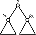
Refer to caption — Figure 1. The tree $T^{h}$ with root $\rho$ ; the left and right sub-trees of $T^{h}$ have roots $\rho_{L}$ and $\rho_{R}$ .

Let $f=\{f_{0},\ldots,f_{h}\}$ be an even pebbling configuration on $T^{h}$ . Let $n(f)=f(T^{h})=\sum_{i=0}^{h}2^{i}f_{i}$ denote the number of pebbles on $T^{h}$ and let $S(f)=\{f_{1},f_{2},\ldots,f_{h}\}$ , the left-shift of $f$ . We can think of $S(f)$ as the pebbling configuration induced by $f$ onto either the right or the left sub-trees of $T^{h}$ . Let $c(f)=\sum_{i=0}^{h}f_{i}$ ; this is the largest number of pebbles that can be amassed by $f$ at the root, $\rho$ .

The reduction of $f$ , denoted by $r(f)$ , is the pebbling configuration on the left sub-tree obtained by transporting the maximum number of pebbles from the right sub-tree and the the root of $T^{h}$ onto the root of the left sub-tree, $\rho_{L}$ . Thus $r(f)=\{f_{0}^{\prime},f_{2},\cdots,f_{h}\},$ where

(6)

f_{0}^{\prime}=f_{1}+\left\lfloor\frac{f_{0}+c(S(f))/2}{2}\right\rfloor

For example, if $f=\{4,2,0,2,0,0\}$ , then $r(f)=\{5,0,2,0,0\}$ .

Lemma 3.1.

A configuration $f$ pebbles $T^{h}$ if and only if at least one pebble can be brought to the root of $T^{h}$ and $r(f)$ pebbles $T^{h-1}$ .

Let $h$ be a positive integer; we define a family of pebbling configurations on the tree $T^{h}$ . Given a list $L$ of length $\ell$ , $\ell\leq h$ , let $\pad_{h}(L)$ be the list of length $h$ obtained by padding $L$ on the right by 0’s. Given a nonnegative integer $k$ such that $s_{k}\leq 2^{h}$ , let

f_{h,k}=\join\left[\{2^{h}-s_{k}\},2\pad_{h}(\langle k\rangle_{M})\right].

A few remarks on this definition are in order. Since $s_{k}\leq 2^{h}$ , the head of $f_{h,k}$ is nonnegative. Furthermore, by Lemma 2.5, the length of $\langle k\rangle_{M}$ is less than or equal to $h-2$ . Thus $f_{h,k}$ is a well-defined pebbling configuration on $T^{h}$ . For $h=5$ and $k=8$ , we observe that $s_{8}=28$ and $\langle 8\rangle_{M}=\{1,0,1\}.$ Therefore, the head of $f_{5,8}$ is $2^{5}-28=4$ and $2\pad_{5}(\langle 8\rangle_{M})=\{2,0,2,0,0\}$ . Consequently, $f_{5,8}=\{4,2,0,2,0,0\}.$

Lemma 3.2.

Let $h$ be a positive integer and let $k$ be a nonnegative integer satisfying $s_{k}\leq 2^{h}$ . Then $n(f_{h,k})=2^{h}-k$ .

Proof.

The result is clear by inspection for $k=0$ . For $k>0$ , let $\langle k\rangle_{M}=\{\varepsilon_{1},\ldots,\varepsilon_{\ell}\}$ . Then $n(f_{h,k})=(2^{h}-s_{k})+2\varepsilon_{1}(2^{1})+\cdots+2\varepsilon_{\ell}(2^{\ell})$ . For each $i\in[\ell]$ , write $2^{i}=M_{i}+1$ . Then $n(f_{h,k})=2^{h}-s_{k}+2k+2\sigma(\langle k\rangle_{M})$ . By Lemma 2.2, $s_{k}=3k+2\sigma(\langle k\rangle_{M})$ . Inserting this into the equation above, we find $n(f_{h,k})=2^{h}-k$ , as was to be shown. ∎

For each positive integer $h$ , let $F_{h}=\{f_{h,k}:s_{k}\leq 2^{h}\}$ . The collections $F_{4}$ and $F_{5}$ are presented in Table 3.

Table 3. The collections

F_{4}

and

F_{5}

$k$	$f_{4,k}$	$n(f_{4,k})$
0	$\{16,0,0,0,0\}$	16
1	$\{11,2,0,0,0\}$	15
2	$\{6,4,0,0,0\}$	14
3	$\{5,0,2,0,0\}$	13
4	$\{0,2,2,0,0\}$	12

$k$	$f_{5,k}$	$n(f_{5,k})$
0	$\{32,0,0,0,0,0\}$	32
1	$\{27,2,0,0,0,0\}$	31
2	$\{22,4,0,0,0,0\}$	30
3	$\{21,0,2,0,0,0\}$	29
4	$\{16,2,2,0,0,0\}$	28
5	$\{11,4,2,0,0,0\}$	27
6	$\{10,0,4,0,0,0\}$	26
7	$\{9,0,0,2,0,0\}$	25
8	$\{4,2,0,2,0,0\}$	24

Lemma 3.3.

Let $h$ be an integer, $h\geq 2$ , and let $f_{k,h}\in F_{h}$ . Then

(a)

$f_{h-1,r(k)}\in F_{h-1}$ , and
(b)

$r(f_{h,k})=f_{h-1,r(k)}$ .

Proof.

For reference,

f_{h-1,r(k)}=\join[\{2^{h-1}-s_{r(k)}\},2\pad_{h-1}(\langle r(k)\rangle_{M})].

By Corollary 2.4, $s_{r(k)}\leq 2^{h-1}$ , which demonstrates that $f_{h-1,r(k)}\in F_{h-1}$ , proving part (a).

To establish part (b), we begin with the calculation of the head of $r(f_{h,k})$ ; see equation (6). The sum of the elements of $2\pad_{h}(\langle k\rangle_{M})$ is $2\sigma(\langle k\rangle_{M})$ . Using Lemma 2.3, the head of $r(f_{h,k})$ is

	$\displaystyle\frac{(2^{h}-s_{k})+\sigma(\langle k\rangle_{M})}{2}+2P_{1}(k)$	$\displaystyle=2^{h-1}-\left(\frac{s_{k}-\sigma(\langle k\rangle_{M})}{2}-2P_{1}(k)\right)$
		$\displaystyle=2^{h-1}-s_{r(k)},$

which shows that $r(f_{h,k})$ and $f_{h-1,r(k)}$ have the same head. We are left to show that the remaining $h-1$ coordinates of $r(f_{h,k})$ and $f_{h-1,r(k)}$ are equal, that is, we must show

(7)

S(2\pad_{h}(\langle k\rangle_{M}))=2\pad_{h-1}(\langle r(k)\rangle_{M}).

But $S(2\pad_{h}(\langle k\rangle_{M}))=2\pad_{h-1}(S(\langle k\rangle_{M}))$ and, by the definition of the reduction of an integer, $S(\langle k\rangle_{M})=\langle r(k)\rangle_{M}$ , which establishes equation (7) and draws our proof to a conclusion. ∎

We are now prepared to state and prove the main result of this section.

Theorem 3.4.

For each nonnegative integer $h$ , $\pi^{*}(T^{h})\leq 2^{h}-k(h).$

Proof.

We begin by showing that each pebbling configuration in $F_{h}$ pebbles $T^{h}$ . For $h=1$ , there is only one pebbling configuration; namely, $f_{1,0}=\{2,0\}$ , and it is easy to see that this configuration pebbles $T^{1}$ . Now let $h\geq 1$ and let us suppose that each pebbling configuration in $F_{h}$ pebbles $T^{h}$ . Let $f_{h+1,k}\in F_{h+1}$ . By Lemma 3.3, $r(f_{h+1,k})=f_{h,r(k)}\in F_{h}$ . Since $f_{h,r(k)}$ pebbles $T^{h}$ , $f_{h+1,k}$ pebbles $T^{h+1}$ .

Let $h$ be a nonnegative integer. To finish our proof, observe that $s_{k(h)}\leq 2^{h}$ ; thus, $f_{h,k(h)}$ pebbles $T^{h}$ . However, by Lemma 3.2, $n(f_{h,k(h)})=2^{h}-k(h)$ , which shows that $\pi^{*}(T^{h})\leq 2^{h}-k(h).$ ∎

4. The lower bound of $\pi^{*}(T^{h})$

Here is the main result of this section.

Theorem 4.1.

For each positive integer $h$ , $\pi^{*}(T^{h})\geq 2^{h}-k(h).$

The proof of this theorem relies on two noteworthy results of Fu and Shiue. According to Lemma 3.3 and Theorem 3.4 of their paper, an optimal symmetric and even pebbling configuration on $T^{h}$ is an optimal pebbling configuration on $T^{h}$ . In effect, our proof of Theorem 4.1 shows that a symmetric and even pebbling configuration on $T^{h-1}$ that contains $2^{h}-k(h)-1$ pebbles cannot pebble $T^{h}$ . Hereafter, we consider only symmetric and even pebbling configurations on $T^{h}$ .

Our next lemma is a simple necessary condition for pebbling.

Lemma 4.2.

If $f=\{f_{0},\ldots,f_{h}\}$ pebbles $T^{h}$ , then

(8)

3n(f)-c(f)\geq 2^{h+1}.

Proof.

The key idea is to treat the pebbles as units of liquid, that is, as infinitely divisible units. In the spirit of pebbling, if a unit of liquid (a pebble) is distance $d$ from a specified leaf, then it can deliver $1/2^{d}$ units of liquid to that leaf. We show that when the inequality (8) is satisfied, then $f$ can deliver a unit of liquid to a specified leaf, which is a necessary condition for delivering a pebble to that leaf.

Let a leaf be specified and consider the path from the root to this leaf. We call this path the spine. Let the rest of the tree be called the remainder. For example, the tree $T^{4}$ , separated into a spine and remainder, is pictured in Figure 2.

The contribution to the leaf from the pebbles in the remainder at distance $h$ from the root is

\frac{2^{h-1}f_{h}}{2^{2h}}+\frac{2^{h-2}f_{h}}{2^{2h-2}}+\cdots+\frac{2^{1}f_{h}}{2^{4}}+\frac{f_{h}}{2^{2}}=\frac{f_{h}M_{h}}{2^{h+1}}.

In general, for $d\in\{1,\ldots,h\}$ , the contribution to the leaf from the remainder from the pebbles at distance $d$ from the root is $f_{d}M_{d}/2^{h+1}$ . In total, the contribution to the leaf from the remainder is

\frac{1}{2^{h+1}}\left(f_{1}M_{1}+\ldots+f_{h}M_{h}\right)=\frac{1}{2^{h+1}}\left(n(f)-c(f)\right).

The contribution to the leaf from the spine is $2n(f)/2^{h+1}.$ Consequently, the total contribution to the leaf from the (liquid) pebbles in the configuration $f$ is $(3n(f)-c(f))/2^{h+1}.$ If $f$ can deliver at least one pebble to the leaf, then $f$ can deliver at least one unit of liquid to the leaf, which completes our proof. ∎

The following sequence plays an important role in the proof of Theorem 4.1. Let $c_{1}=2$ and, for $k\geq 2$ , let $c_{k}=3(2^{k})-2$ . An important feature of this sequence is contained in the next lemma, which we state without proof.

Lemma 4.3.

For $i\geq 1$ , $3c_{1}+c_{2}+c_{3}+\cdots+c_{i}=c_{i+1}-(i+1)2.$

Let $h$ and $m$ be positive integers with $m<2^{h+2}$ . The binary expansion of $m$ is $m=\delta_{0}+2^{1}\delta_{1}+2^{2}\delta_{2}+\cdots+\delta_{h+1}2^{h+1},$ where $\delta_{i}\in\{0,1\}$ for each integer $i$ , $0\leq i\leq h+1$ . The configuration

\psi_{h,m}=\{\delta_{0}+2\delta_{1},2\delta_{2},\ldots,2\delta_{h+1}\}

is an even, symmetric pebbling configuration on $T^{h}$ containing $m$ pebbles. It is easy to show that $\psi_{h,m}$ maximizes $3n(f)-c(f)$ among the set of even, symmetric pebbling configurations $f$ on $T^{h}$ containing $m$ pebbles. Let $t_{m}=3n(\psi_{h,m})-c(\psi_{h,m})$ ; it can be shown that

(9)

t_{m}=(\delta_{0}+\delta_{1}2^{1})c_{1}+\delta_{2}c_{2}+\cdots+\delta_{h+1}c_{h+1}.

Finally, here is the proof of Theorem 4.1, the main result of this section.

Proof of Theorem 4.1.

The result is true for $h=1$ by inspection. Let $h\geq 2$ be given. We show that $t_{2^{h}-k(h)-1}<2^{h+1}$ , which, according to Lemma 4.2, proves the theorem.

Let $2^{h}=r+\varepsilon_{1}\mu_{1}+\cdots+\varepsilon_{\ell}\mu_{\ell}$ be the $\mu$ -expansion of $2^{h}$ . Then $k(h)=\varepsilon_{1}M_{1}+\cdots+\varepsilon_{\ell}M_{\ell}$ and $s_{k(h)}=\varepsilon_{1}\mu_{1}+\cdots+\varepsilon_{\ell}\mu_{\ell}$ . Thus

	$\displaystyle 2^{h}-k(h)$	$\displaystyle=r+\varepsilon_{1}(\mu_{1}-M_{1})+\cdots+\varepsilon_{\ell}(\mu_{\ell}-M_{\ell})$
		$\displaystyle=r+\varepsilon_{1}2^{2}+\cdots+\varepsilon_{\ell}2^{\ell+1}$

Our proof is divided into cases, depending on whether or not $r=0$ .

First, let us suppose that $r=0$ and that $\varepsilon_{i}\neq 2$ for each $i\in[\ell]$ in the $\mu$ -expansion of $2^{h}$ . Then the binary expansion of $2^{h}-k(h)$ is $\varepsilon_{1}2^{2}+\cdots+\varepsilon_{\ell}2^{\ell+1}$ and therefore

	$\displaystyle t_{2^{h}-{k(h)}}$	$\displaystyle=\varepsilon_{1}c_{2}+\varepsilon_{2}c_{3}+\cdots+\varepsilon_{\ell}c_{\ell+1}$
		$\displaystyle=2(\varepsilon_{1}\mu_{1}+\varepsilon_{2}\mu_{2}+\cdots+\varepsilon_{\ell}\mu_{\ell})$
		$\displaystyle=2s_{k(h)}$
		$\displaystyle=2^{h+1}.$

Since the sequence $\{t_{k}\}$ is strictly increasing, $t_{2^{h}-{k(h)}-1}<2^{h+1}$ .

Next, let us suppose that $r=0$ but that $\varepsilon_{j}=2$ for some $j\in[\ell]$ in the $\mu$ -expansion of $2^{h}$ . In particular, this implies that $\varepsilon_{i}\in\{0,1\}$ for each integer $i\in\{j+1,\ldots,\ell\}$ . Then

2^{h}-{k(h)}=2(2^{j+1})+\varepsilon_{j+1}2^{j+2}+\cdots\varepsilon_{\ell}2^{\ell+1}.

Therefore, the binary expansion of $2^{h}-k(h)-1$ is

1+2+2^{2}+\cdots+2^{j}+2^{j+1}+\varepsilon_{j+1}2^{j+2}+\cdots+\varepsilon_{\ell}2^{\ell+1}

hence

t_{2^{h}-{k(h)}-1}=3c_{1}+c_{2}+\cdots+c_{j}+c_{j+1}+\varepsilon_{j+1}c_{j+2}+\cdots+\varepsilon_{\ell}c_{\ell+1}.

By Lemma 4.3, we may conclude

	$\displaystyle t_{2^{h}-{k(h)}-1}$	$\displaystyle=2c_{j+1}+\varepsilon_{j+1}c_{j+2}+\cdots\varepsilon_{\ell}c_{\ell+1}-(j+1)2$
		$\displaystyle=2(2\mu_{j}+\varepsilon_{j+1}\mu_{j+1}+\cdots\varepsilon_{\ell}\mu_{\ell})-(j+1)2$
		$\displaystyle=2s_{k(h)}-(j+1)2$
		$\displaystyle=2^{h+1}-(j+1)2.$

In particular, this shows that $t_{2^{h}-{k(h)}-1}<2^{h+1}$ , as was to be shown.

Lastly, let us assume that $r\in\{1,2,3,4\}$ in the $\mu$ -expansion of $2^{h}$ . This implies that $\varepsilon_{i}\in\{0,1\}$ for each $i\in[\ell]$ . Then $r-1\in\{0,1,2,3\}$ and the binary expansion of $2^{h}-{k(h)}-1$ is

(r-1)+\varepsilon_{1}2^{2}+\varepsilon_{2}2^{3}+\cdots+\varepsilon_{\ell}2^{\ell+1}.

Thus,

	$\displaystyle t_{2^{h}-{k(h)}-1}$	$\displaystyle=2(r-1)+\varepsilon_{1}c_{2}+\varepsilon_{2}c_{3}+\cdots+\varepsilon_{\ell}c_{\ell+1}$
		$\displaystyle=2(r-1)+\varepsilon_{1}2\mu_{1}+\varepsilon_{2}2\mu_{3}+\cdots+\varepsilon_{\ell}2\mu_{\ell}$
		$\displaystyle=2\left((r-1)+\varepsilon_{1}\mu_{1}+\varepsilon_{2}\mu_{3}+\cdots+\varepsilon_{\ell}\mu_{\ell}\right)$
		$\displaystyle=2^{h+1}-2,$

as was to be shown. ∎

5. Asymptotic analysis of $k(h)$

In this section we study the asymptotic behavior of $k(h)$ as $h\to\infty$ . Given a positive integer $m$ , let $s^{-1}(m)=\max\{n:s_{n}\leq m\}.$ In this notation, $k(h)=s^{-1}(2^{h}).$ Our first step is to develop a formula for the inverse of $s$ .

Let $m$ be a positive integer with $\mu$ -expansion $m=r+\varepsilon_{1}\mu_{1}+\cdots+\varepsilon_{\ell}\mu_{\ell}.$ Let $\phi(m)=\varepsilon_{1}+\cdots+\varepsilon_{\ell}$ . For example, the $\mu$ -expansions of 236 and 253 are $2\mu_{2}+\mu_{3}+\mu_{6}$ and $4+\mu_{2}+\mu_{4}+\mu_{6}$ ; thus $\phi(236)=4$ and $\phi(253)=3$ .

Theorem 5.1.

Given a positive integer $m$ , there exists an integer $r\in\{0,1,2,3,4\}$ such that $m-r=3s^{-1}(m)+2\phi(m)$ .

Proof.

Let $m=r+\varepsilon_{1}\mu_{1}+\cdots+\varepsilon_{\ell}\mu_{\ell}$ be the $\mu$ -expansion of $m$ . Since $\mu_{i}=3M_{i}+2$ for each positive integer $i$ ,

m-r=3(\varepsilon_{1}M_{1}+\cdots+\varepsilon_{\ell}M_{\ell})+2(\varepsilon_{1}+\ldots+\varepsilon_{\ell}).

The right-hand side is $3s^{-1}(m)+2\phi(m)$ , as was to be shown. ∎

Let $h$ be a positive integer. Since $k(h)=s^{-1}(h)$ , Theorem 5.1 asserts that there exists an integer $r\in\{0,1,2,3,4\}$ such that

(10)

k(h)=2^{h}/3-2\phi(2^{h})/3-r/3.

Therefore, in order to understand the asymptotic behavior of $k(h)$ , we need to investigate the asymptotic behavior of $\phi(2^{h})$ . To this end, let

(11)

\alpha(h)=\frac{2\phi(2^{h})-(h+2)}{\log_{2}(h+2)}.

We prove the following theorem.

Theorem 5.2.

For $h\geq 2$ , $-1\leq\alpha(h)\leq 1.$ In addition, $\liminf_{h\to\infty}\alpha(h)=-1$ and $\limsup_{h\to\infty}\alpha(h)=1.$

Proof.

Let $h$ be an integer, $h\geq 2$ . Let $x^{*}=x^{*}(h)$ be the root of the equation

(12)

h-2x-1-\log_{2}(x+1)=0,

and let $j^{*}=\lceil x^{*}\rceil.$ Then $j^{*}=\min\{j:j\geq 2^{h-2j-1}-1\}.$

First we develop the $\mu$ -expansion of $2^{h}$ and show that $\phi(2^{h})\geq j^{*}+1$ . To get started, notice that $\mu_{h-2}\leq 2^{h}<\mu_{h-1}$ and that $2^{h}-\mu_{h-2}=2^{h-2}+1$ . We can continue this process of successive subtractions $j^{*}$ times, obtaining

2^{h}-\sum_{i=1}^{j^{*}}\mu_{h-2i}=2^{h-2j^{*}}+j^{*}.

At this point, the simple pattern of subtractions is disrupted; the next subtraction is $\mu_{h-2j^{*}-1}$ , which yields

2^{h}-\mu_{h-2}-\cdots-\mu_{h-2j^{*}}-\mu_{h-2j^{*}-1}=A,

where $A=j^{*}-\left(2^{h-2j^{*}-1}-1\right).$ Thus $\phi(2^{h})=j^{*}+1+\phi(A)$ .

An analysis of equation (12) reveals that

j^{*}+1\geq\frac{1}{2}(h+2)-\frac{\log_{2}(h+2)}{2}.

Likewise, $A\leq 2^{h-2j^{*}}+2^{h-2j^{*}-1}$ hence $0\leq\phi(A)\leq h-2j^{*}-1$ and we may conclude that

(h+2)-\log_{2}(h+2)\leq 2\phi(2^{h})\leq(h+2)+\log_{2}(h+2),

or $-1\leq\alpha(h)\leq 1$ .

We are left to prove the claims about the limits inferior and superior of $\alpha(h)$ . We consider two families of trees.

(a)

Let $h=h_{k}=2^{k+1}+k-1$ . Then $j^{*}=j^{*}_{k}=2^{k}-1$ and

$2^{h}-\sum_{i=1}^{j^{*}}\mu_{h-2i}=\mu_{h-2j^{*}-1}.$

Accordingly, $\phi(2^{h})=j^{*}+1=2^{k}$ , and $\lim_{k\to\infty}\alpha(h_{k})=-1,$ which shows $\liminf_{h\to\infty}\alpha(h)=-1$ .

(b)

Let $h=h_{k}=2^{k+2}-k$ . Then $j^{*}=j^{*}_{k}=2^{k+1}-k$ and

	$\displaystyle 2^{h}-\sum_{i=1}^{j^{*}}\mu_{h-2i}$	$\displaystyle=2^{k}+(2^{k+1}-k)$
		$\displaystyle=\mu_{k-1}+\mu_{k-2}+\cdots+\mu_{2}+2\mu_{1}.$

Thus $\phi(2^{h})=j^{*}+k=2^{k+1}$ and $\lim_{k\to\infty}\alpha(h_{k})=1$ , which shows that $\limsup_{h\to\infty}\alpha(h)=1$ .

Our proof is complete. ∎

By combining equations (10) and (11), we find that

k(h)=\frac{1}{3}(2^{h})-\frac{1}{3}(h+2)-\frac{1}{3}\alpha(h)\log_{2}(h+2)+O(1).

The families of trees presented at the end of the proof reveal some interesting examples of optimal pebblings. In case (a), the first level that contains any pebbles is $k$ and thereafter, the pebbling configuration follows a regular, alternating pattern. In other words, the top of the tree is empty. In case (b), each of the levels 1 through $k-1$ contain pebbles and thereafter the pebbling configuration follows a regular alternating pattern. In other words, the top of the tree, except for the root itself, is full.

Let levels 0 through $h-2j^{*}-2$ designate the top of $T^{h}$ and let the remaining levels be called the bottom of the tree $T^{h}$ . We can see that the bottom of the tree $T^{h}$ starts at approximately level

h-2j^{*}-1\sim\log_{2}(h/2+1).

Our analysis reveals that an optimal pebbling of $T^{h}$ is regular on the bottom: there are 2 or 4 pebbles at level $h-2j^{*}-1$ and 2 pebbles in each of the levels $h-2k$ , $k\in\{1,\ldots,j^{*}\}$ . The top of $T^{h}$ , however, may vary from full to empty.

6. Connections with the Connolly-Fox sequence

Recall from §1 that the Conolly-Fox sequence $\{c_{n}\}$ satisfies the recurrence relation (2) with initial conditions $c(1)=1$ and $c(2)=2$ . We will prove the following theorem.

Theorem 6.1.

For each positive integer $n$ , $s_{n}=4c_{n}+n$ .

Proof.

We begin by defining a list of numbers composed entirely of 0s and 1s. Let $D_{1}=\{1\}$ . We define successive lists recursively: for each integer $k$ , $k\geq 2$ , let $D_{k}=\join[D_{k-1},D_{k-1},\{0\}].$ The lists $D_{1}$ through $D_{4}$ are collected in Table 4.

Table 4. The lists

D_{1}

through

D_{4}

$k$	$D_{k}$
1	{1}
2	{1, 1, 0}
3	{1, 1, 0, 1, 1, 0, 0}
4	{1, 1, 0, 1, 1, 0, 0, 1, 1, 0, 1, 1, 0, 0, 0}

Let $D$ be the limit of this sequence of lists and, for each positive integer $n$ , let $d_{n}$ denote the $n$ th element of $D$ . The sequence $\{d_{n}\}$ is the sequence of differences in the Conolly-Fox sequence; see OEIS, A079559 [17]. Thus, for each positive integer $n$ , $c_{n}=d_{1}+\cdots+d_{n}$ . The initial terms of the sequences $\{d_{n}\}$ and $\{c_{n}\}$ are presented in Table 5.

Table 5. The initial terms of

\{d_{n}\}

and

\{c_{n}\}

$n$	1	2	3	4	5	6	7	8	9	10	11	12	13	14	15
$d_{n}$	1	1	0	1	1	0	0	1	1	0	1	1	0	0	0
$c_{n}$	1	2	2	3	4	4	4	5	6	6	7	8	8	8	8

Recall the sequence $\{a_{n}\}$ defined in §1; see Table 2. For each positive integer $n$ , it is easy to see that $a_{n}=4d_{n}+1$ and therefore $s_{n}=4c_{n}+n$ , as was to be shown. ∎

References

[1] Robert A. Beeler, Teresa W. Haynes, Michael A. Henning, and Rodney Keaton, Total domination cover rubbling, Discrete Appl. Math. 283 (2020), 133–141. MR 4114886
[2] Robert A. Beeler, Teresa W. Haynes, and Rodney Keaton, Domination cover rubbling, Discrete Appl. Math. 260 (2019), 75–85. MR 3944610
[3] Robert A. Beeler, Teresa W. Haynes, and Kyle Murphy, 1-restricted optimal rubbling on graphs, Discuss. Math. Graph Theory 39 (2019), no. 2, 575–588. MR 3900331
[4] Christopher Belford and Nándor Sieben, Rubbling and optimal rubbling of graphs, Discrete Math. 309 (2009), no. 10, 3436–3446. MR 2528207
[5] Mustapha Chellali, Teresa W. Haynes, Stephen T. Hedetniemi, and Thomas M. Lewis, Restricted optimal pebbling and domination in graphs, Discrete Appl. Math. 221 (2017), 46–53. MR 3612586
[6] Fan R. K. Chung, Pebbling in hypercubes, SIAM J. Discrete Math. 2 (1989), no. 4, 467–472. MR 1018531
[7] Thomas H. Cormen, Charles E. Leiserson, Ronald L. Rivest, and Clifford Stein, Introduction to algorithms, second ed., MIT Press, Cambridge, MA; McGraw-Hill Book Co., Boston, MA, 2001. MR 1848805
[8] A. Czygrinow, G. Hurlbert, G. Y. Katona, and L. F. Papp, Optimal pebbling number of graphs with given minimum degree, Discrete Appl. Math. 260 (2019), 117–130. MR 3944614
[9] Nathan Fox, Trees, fibonacci numbers, and nested recurrences, https://youtu.be/Y4rC5TEW_TY, March 2019.
[10] Hung-Lin Fu and Chin-Lin Shiue, The optimal pebbling number of the complete $m$ -ary tree, Discrete Math. 222 (2000), no. 1-3, 89–100. MR 1771391
[11] Ze-Tu Gao and Jian-Hua Yin, The optimal pebbling of spindle graphs, Open Math. 17 (2019), no. 1, 582–587. MR 4031681
[12] Ervin Győri, Gyula Y. Katona, and László F. Papp, Optimal pebbling and rubbling of graphs with given diameter, Discrete Appl. Math. 266 (2019), 340–345. MR 3991624
[13] by same author, Optimal pebbling number of the square grid, Graphs Combin. 36 (2020), no. 3, 803–829. MR 4090527
[14] Ervin Győri, Gyula Y. Katona, László F. Papp, and Casey Tompkins, The optimal pebbling number of staircase graphs, Discrete Math. 342 (2019), no. 7, 2148–2157. MR 3957918
[15] David S. Herscovici, Benjamin D. Hester, and Glenn H. Hurlbert, Optimal pebbling in products of graphs, Australas. J. Combin. 50 (2011), 3–24. MR 2829275
[16] Glenn Hurlbert, General graph pebbling, Discrete Appl. Math. 161 (2013), no. 9, 1221–1231. MR 3030615
[17] OEIS Foundation Inc., The on-line encyclopedia of integer sequences, 2021.
[18] Lior Pachter, Hunter S. Snevily, and Bill Voxman, On pebbling graphs, Proceedings of the Twenty-sixth Southeastern International Conference on Combinatorics, Graph Theory and Computing (Boca Raton, FL, 1995), vol. 107, 1995, pp. 65–80. MR 1369255
[19] Chin-Lin Shiue, Capacity restricted optimal pebbling in graphs, Discrete Appl. Math. 260 (2019), 284–288. MR 3944631
[20] by same author, Distance restricted optimal pebbling in cycles, Discrete Appl. Math. 279 (2020), 125–133. MR 4092629
[21] Chin-Lin Shiue, Hung-Hsing Chiang, Mu-Ming Wong, and H. M. Srivastava, The optimal $t$ -pebbling number of a certain complete $m$ -ary tree, Rev. R. Acad. Cienc. Exactas Fís. Nat. Ser. A Mat. RACSAM 113 (2019), no. 3, 2889–2910. MR 3956289
[22] Chin-Lin Shiue and Hung-Lin Fu, The optimal pebbling number of the caterpillar, Taiwanese J. Math. 13 (2009), no. 2A, 419–429. MR 2499997
[23] Chenxiao Xue and Carl Yerger, Optimal pebbling on grids, Graphs Combin. 32 (2016), no. 3, 1229–1247. MR 3489733
[24] Yongsheng Ye, Mei Liu, and Jie Gao, The optimal pebbling number of square of paths and cycles, Ars Combin. 114 (2014), 363–371. MR 3203678

Optimal Pebbling of Complete Binary Trees and a Meta-Fibonacci Sequence

1. Introduction

1.1. Prologue

1.2. Results

1.3. Background and related work

2. Some essential lemmas

Lemma 2.1.

Proof.

Lemma 2.2.

Proof.

Lemma 2.3.

Proof.

Corollary 2.4.

Lemma 2.5.

Proof.

3. The upper bound of π∗​(Th)\pi^{*}(T^{h})

Lemma 3.1.

Lemma 3.2.

Proof.

Lemma 3.3.

Proof.

Theorem 3.4.

Proof.

4. The lower bound of π∗​(Th)\pi^{*}(T^{h})

Theorem 4.1.

Lemma 4.2.

Proof.

Lemma 4.3.

Proof of Theorem 4.1.

5. Asymptotic analysis of k⁡(h)k(h)

Theorem 5.1.

Proof.

Theorem 5.2.

Proof.

6. Connections with the Connolly-Fox sequence

Theorem 6.1.

Proof.

References

3. The upper bound of $\pi^{*}(T^{h})$

4. The lower bound of $\pi^{*}(T^{h})$

5. Asymptotic analysis of $k(h)$