PoWareMatch: a Quality-aware Deep Learning Approach to Improve Human Schema Matching – Technical ReportDOI: 10.1145/1122445.1122456Journal: JDIQVolume: xxxxxx3

When it comes to humans performing a matching task, decisions regarding correspondences among data sources are made sequentially. To illustrate, consider Figure 1(a), presenting two simplified purchase order schemata adopted from (Do and Rahm 2002). PO₁ has four attributes (foreign keys are ignored for simplicity): purchase order’s number (poCode), timestamp (poDay and poTime) and shipment city (city). PO₂ has three attributes: order issuing date (orderDate), order number (orderNumber), and shipment city (city). A human matching sequence is given by the orderly annotated double-arrow edges. For example, a matching decision that poDay in PO₁ corresponds to orderNumber in PO₂ is the second decision made in the process.

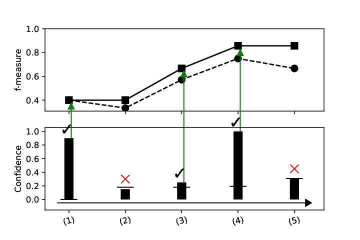
The traditional view on human matching accepts human decisions as a ground truth (possibly subject to validation by additional human matchers) and thus the outcome match is composed of all the correspondences selected (or validated) by the human matcher. Figure 1(b) illustrates this view using the decision making process of Figure 1(a). The x-axis represents the ordering according to which correspondences were selected. The dashed line at the top illustrates the changes to the f-measure (see Section 2.1 for f-measure’s definition) as more decisions are added, starting with an f-measure of $0.4$, dropping slightly and then rising to a maximum of $0.75$ before dropping again as a result of the final human matcher decision.

In this work we offer an alternative approach that analyzes the sequential nature of human matching decision making and confidence values humans share to monitor performance and modify decisions accordingly. In particular, we set a dynamic threshold (marked as a horizontal line for each decision at the bottom of Figure 1(b)), that takes into account previous decisions with respect to the quality of the match (f-measure in this case). Comparing the threshold to decision confidence (marked as bars in the figure), the algorithm determines whether a human decision is included in the match (marked using a ✓sign and an arrow to indicate inclusion) or not (marked as a red $X$). A process-aware approach, for example, accepts the third decision that poTime in PO₁ corresponds with orderDate in PO₂ made with a confidence of $0.25$ while rejecting the fifth decision that poDay in PO₁ corresponds with orderNumber in PO₂, despite the higher confidence of $0.3$. The f-measure of this approach, as illustrated by the solid line at the top of the figure, demonstrates a monotonic non-decreasing behavior with a final high value of $0.86$.

More on the method, assumptions and how the acceptance threshold is set can be found in Section 4.1. Section 4.2 introduces a deep learning methodology to calibrate matching decisions, aiming to optimize the quality of a match with respect to a target evaluation measure.

In this work we focus on (real-world) human matching with the overarching goal of improving matching quality using deep learning. Specifically, we analyze a setting where human matchers interact directly with a pair of schemata, aiming to find accurate correspondences between them. In such a setting, the matching decisions emerge as a process (matching-as-a-process, see Figure 1) and can be monitored accordingly to advocate the quality of a current outcome match. In what follows, we characterize the dynamics of matching-as-a-process with respect to common quality evaluation measures, namely, precision, recall, and f-measure, by defining a monotonic evaluation measure and its probabilistic derivative. We show conditions under which precision, recall and f-measure are monotonic and identify correspondences that their addition to a match improves on its quality. These conditions provide solid, theoretically grounded decision making, leading to the design of a step-wise matching algorithm that uses human confidence to construct a quality-aware match, taking into account the process of matching.

The theoretical setting described above requires human matchers to offer unbiased matching (which we formally define in this paper), assuming human matchers are experts in matching. This is, unfortunately, not always the case and human matchers were shown to have cognitive biases when matching (Ackerman et al. 2019), which may lead to poor decision making. Rather than aggregately judge human matcher proficiency and discard those that may seem to provide inferior decisions, we propose to directly overcome human biases and accept only high-quality decisions. To this end, we introduce PoWareMatch (Process aWare Matcher), a quality-aware deep learning approach to calibrate and filter human matching decisions and combine them with algorithmic matching to provide better match results. We performed an empirical evaluation with over $200$ human matchers to show the effectiveness of our approach in generating high quality matches. In particular, since we adopt a supervised learning approach, we also demonstrate the applicability of PoWareMatch over a set of (unknown) human matchers over an (unfamiliar) matching problem.

The paper offers the following four specific contributions:

1. (1)

   A formal framework for evaluating the quality of (human) matching-as-a-process using the well known evaluation measures of precision, recall, and f-measure (Section 3).

2. (2)

   A matching algorithm that uses confidence to generate a process-aware match with respect to an evaluation measure that dictates its quality (Section 4.1).

3. (3)

   PoWareMatch (Section 4.2), a matching algorithm that uses a deep learning model to calibrate human matching decisions (Section 4.3) and algorithmic matchers to complement human matching (Section 4.4).

4. (4)

   An empirical evaluation showing the superiority of our proposed solution over state-of-the-art in schema matching using known benchmarks (Section 5).

Section 2 provides a matching model and discusses algorithmic and human matching. The paper is concluded with related work (Section 6), concluding remarks and future work (Section 7).

Let $S,S^{\prime}$ be two schemata with attributes $\{a_{1},a_{2},\dots,a_{n}\}$ and $\{b_{1},b_{2},\dots,b_{m}\}$, respectively. A matching model matches $S$ and $S^{\prime}$ by aligning their attributes using matchers that utilize matching cues such as attribute names, instances, schema structure, etc. (see surveys, e.g., (Bernstein et al. 2011) and books, e.g., (Gal 2011)).

A matcher’s output is conceptualized as a matching matrix $M(S,S^{\prime})$ (or simply $M$), as follows.

Let $M^{*}$ be a reference matrix. $M^{*}$ is a binary matrix, such that $M^{*}_{ij}=1$ whenever $a_{i}\in{S}$ and $b_{j}\in{S^{\prime}}$ correspond and $M^{*}_{ij}=0$ otherwise. A reference match, denoted $\sigma^{*}$, is given by $\sigma^{*}=\{M^{*}_{ij}|M^{*}_{ij}=1\}$. Reference matches are typically compiled by domain experts over the years in which a dataset has been used for testing. $G_{\sigma^{*}}:\Sigma\rightarrow[0,1]$ is an evaluation measure, assigning scores to matches according to their ability to identify correspondences in the reference match. Whenever the reference match is clear from the context, we shall refer to $G_{\sigma^{*}}$ simply as $G$. We define the precision ($P$) and recall ($R$) evaluation measures (Bellahsene et al. 2011b), as follows:

The f-measure ($F_{1}$ score), $F(\sigma)$, is calculated as the harmonic mean of $P(\sigma)$ and $R(\sigma)$.

The schema matching problem is expressed as follows.

Matching is often a stepped procedure applying algorithms, rules, and constraints. Algorithmic matchers can be classified into those that are applied directly to the problem (first-line matchers – 1LMs) and those that are applied to the outcome of other matchers (second-line matchers – 2LMs). 1LMs receive (typically two) schemata and return a matching matrix, in which each entry $M_{ij}$ captures the similarity between attributes $a_{i}$ and $b_{j}$. 2LMs receive (one or more) matching matrices and return a matching matrix using some function $f(M)$ (Gal 2011). Among the 2LMs, we term decision makers those that return a binary matrix as an output, from which a match $\sigma$ is derived, by maximizing $f(M)$, as a solution to Problem 1.

To illustrate the algorithmic matchers in the literature, consider three 1LMs, namely Term, WordNet, and Token Path and three 2LMs, namely Dominants, Threshold($\nu$), and Max-Delta($\delta$). Term (Gal 2011) compares attribute names to identify syntactically similar attributes (e.g., using edit distance and soundex). WordNet uses abbreviation expansion and tokenization methods to generate a set of related words for matching attribute names (Gawinecki 2009). Token Path (Peukert et al. 2011) integrates node-wise similarity with structural information by comparing the syntactic similarity of full paths from root to a node. Dominants (Gal 2011) selects correspondences that dominate all other correspondences in their row and column. Threshold($\nu$) and Max-Delta($\delta$) are selection rules, prevalent in many matching systems (Do and Rahm 2002). Threshold($\nu$) selects those entries $(i,j)$ having $M_{ij}\geq{\nu}$. Max-Delta($\delta$) selects those entries that satisfy: $M_{ij}+\delta\geq{\max_{i}}$, where $\max_{i}$ denotes the maximum match value in the $i$’th row.

In this work, we examine human schema matching as a decision making process. Different from a binary crowdsourcing setting (e.g., (Zhang et al. 2018)), in which the matching task is typically reduced into a set of (binary) judgments regarding specific correspondences (see related work, Section 6), we focus on human matchers that perform a matching task in its entirety, as illustrated in Figure 1.

Human schema matching is a complex sequential decision making process of interrelated decisions. Attribute of multiple schemata are examined to decide whether and which attributes correspond. Humans either validate an algorithmic result or locate a candidate attribute unassisted, possibly relying upon superficial information such as string similarity of attribute names or exploring information such as data-types, instances, and position within the schema tree. The decision whether to explore additional information relies upon self-monitoring of confidence.

Human schema matching has been recently analyzed using metacognitive psychology (Ackerman et al. 2019), a discipline that investigates factors impacting humans when performing knowledge intensive tasks (Barsalou 2014). The metacognitive approach (Bjork et al. 2013), traditionally applied for learning and answering knowledge questions, highlights the role of subjective confidence in regulating efforts while performing tasks. Metacognitive research shows that subjective judgments (e.g., confidence) regulate the cognitive effort invested in each decision (e.g., identifying a correspondence) (Metcalfe and Finn 2008; Ackerman and Thompson 2017). In what follows, we model human matching as a sequence of decisions regarding element pairs, each assigned with a confidence level. In this work we assume that human matchers interact directly with the matching problem, selecting correspondences given a pair of schemata. Within this process, we directly query their (subjective) confidence level regarding a selected correspondence, which essentially reflects the ongoing monitoring and final subjective assessment of chances of success (Bjork et al. 2013; Ackerman and Thompson 2017). The dynamics of human matching decision making process is modeled using a decision history $H$, as follows.

Each decision $h_{t}\in H$ records a matching decision confidence ($h_{t}.c$) concerning an element pair ($h_{t}.e=\left(a_{i},b_{j}\right)$) at time $t$ ($h_{t}.t$). Timestamps induce a total order over $H$’s elements.

A matching matrix, which may serve as a solution of the human matcher to Problem 1, can be created from a matching history by assigning the latest confidence to the respective matrix entry. Given an element pair $e=\left(a_{i},b_{j}\right)$, we denote by $h_{max}^{e}$ the latest decision making in $H$ that refers to $e$ and compute a matrix entry as follows:

where $M_{ij}=\varnothing$ means that $M_{ij}$ was not assigned a confidence value. Whenever clear from the context, we refer to a confidence value ($h_{t}.c$) assigned to an element pair $\left(a_{i},b_{j}\right)$, simply as $M_{ij}$.

In this work we seek a solution to Problem 1 that takes into account the quality of a match wrt an evaluation measure $G$ and a decision history $H$. Therefore, we next analyze the well-known measures, namely precision, recall, and f-measure in the context of matching-as-a-process.

Given two matches (Definition 1) $\sigma$ and $\sigma^{\prime}$ that are a result of some sequential decision making such that $\sigma\subseteq\sigma^{\prime}$, we define their interrelationship using their monotonic behavior with respect to an evaluation measure $G$ ($P$, $R$, or $F$, see Eq. 1). For the remainder of the section, we denote by $\Sigma^{\subseteq}$ the set of all match pairs in $\Sigma\times\Sigma$ such that the first match is a subset of the second: $\Sigma^{\subseteq}=\{(\sigma,\sigma^{\prime})\in\Sigma\times\Sigma:\sigma\subseteq\sigma^{\prime}\}$ and use $\Delta_{\sigma,\sigma^{\prime}}=\sigma^{\prime}\setminus\sigma$ ($\Delta$, when clear from the context) to denote the set of correspondences that were added to $\sigma$ to generate $\sigma^{\prime}$.

In Definition 1, we use $\Sigma^{2}$ as a representative subspace of $\Sigma^{\subseteq}$, which was defined above. According to Definition 1, an evaluation measure $G$ is monotonically increasing (MIEM) if by adding correspondences to a match, we do not reduce its value. It is fairly easy to infer that recall is an MIEM over all match pairs in $\Sigma^{\subseteq}$ and precision and f-measure are not, unless some strict conditions hold. To guarantee such conditions, we define two subsets, $\Sigma^{P}=\{(\sigma,\sigma^{\prime})\in\Sigma^{\subseteq}:P(\sigma)\leq P(\Delta)\}$ and $\Sigma^{F}=\{(\sigma,\sigma^{\prime})\in\Sigma^{\subseteq}:0.5\cdot F(\sigma)\leq P(\Delta)\}$. The former represents a subset of all match pairs for which the precision of the added correspondences ($P(\Delta)$) is at least as high as the precision of the first match ($P(\sigma)$). The latter compares between the added correspondences ($P(\Delta)$) and the f-measure of the first match ($F(\sigma)$). We use these two subspaces in the following theorem to summarize the main dynamic properties of the evaluation measures of precision, recall, and f-measure.²² 2 The proof of Theorem 2 is given in Appendix A.

The analysis of Section 3.1 lays the groundwork for a principled matching process that continuously improves on the evaluation measure of choice. The conditions set forward use knowledge of, first, the evaluation outcome of the match performed thus far ($G(\sigma)$), and second, the evaluation score of the additional correspondences ($G(\Delta)$). While such knowledge can be extremely useful, it is rarely available during the matching process. Therefore, we next provide a relaxed setting, where $G(\sigma)$ and $G(\Delta)$ are probabilistically known (Section 3.3 provides an approximation using human confidence). For simplicity, we restrict our analysis to matching processes where a single correspondence is added at a time. We denote by $\Sigma^{\subseteq_{1}}=\{(\sigma,\sigma^{\prime})\in\Sigma^{\subseteq}:|\sigma^{\prime}|-|\sigma|=1\}$ the set of all match pairs $(\sigma,\sigma^{\prime})$ in $\Sigma^{\subseteq}$ where $\sigma^{\prime}$ is generated by adding a single correspondence to $\sigma$. The discussion below can be extended (beyond the scope of this work) to adding multiple correspondences at a time.

We start with a characterization of correspondences whose addition to a match improves on the match evaluation. Recall that $\Delta$ represents the marginal set of correspondences that were added to the match. Following the specification of $\Sigma^{\subseteq_{1}}$, we let $\Delta$ represent a single correspondence ($|\Delta|=1$), which is the result of multiple match pairs $(\sigma,\sigma^{\prime})\in\Sigma^{\subseteq_{1}}$ such that $\Delta=\sigma^{\prime}\setminus\sigma$.

A local annealer is a single correspondence that is guaranteed to improve the performance of any match within a specific match pair subset. We now connect the MIEM property of an evaluation measure $G$ (Definition 1) with the annealing property of a match delta $\Delta$ (Definition 3) with respect to a specific match $\sigma^{\prime}$.³³ 3 All proofs are provided in Appendix A

Proposition 1 demonstrates the importance of defining the appropriate subset of matches that satisfy monotonicity. Together with Theorem 2, the following immediate corollary can be deduced.

Corollary 1 indicates which correspondence should be added to a match to improve its quality with respect to an evaluation measure of choice, according to the respective condition.

Assume now that the value of $G$, applied to a match $\sigma$, is not deterministically known. Rather, $G(\sigma)$ is a random variable with an expected value of $E(G(\sigma))$. We extend Definition 3 as follows.

We now define conditions (match subspaces) under which a correspondence is a probabilistic local annealer for recall ($R$), precision ($P$), and f-measure ($F$). Let ${\rm I\!I}_{\{\Delta\in\sigma^{*}\}}$ be an indicator function, returning a value of $1$ whenever $\Delta$ is a part of the reference match and $0$ otherwise.

Using ${\rm I\!I}_{\{\Delta\in\sigma^{*}\}}$, we define the probability that $\Delta$ is correct: $Pr\{\Delta\in\sigma^{*}\}\equiv Pr\{{\rm I\!I}_{\{\Delta\in\sigma^{*}\}}=1\}$.

Lemma 4 is the probabilistic counterpart of Lemma 3 (see Appendix A).

Using the following subsets: $\Sigma^{E(P)}=\{(\sigma,\sigma^{\prime})\in\Sigma^{\subseteq_{1}}:E(P(\sigma))\leq Pr\{\Delta\in\sigma^{*}\}\}$ and $\Sigma^{E(F)}=\{(\sigma,\sigma^{\prime})\in\Sigma^{\subseteq_{1}}:0.5\cdot E(F(\sigma))\leq Pr\{\Delta\in\sigma^{*}\}\}$, we extend Theorem 2 to the probabilistic setting.⁴⁴ 4 The proof of Theorem 6 is given in Appendix A.

Intuitively, using Theorem 6 one can infer those correspondences, whose addition to the current match improves its quality. For example, if a reference match contains $12$ correspondences and a current match contains $9$ correct correspondences (i.e., correspondences that are included in the reference match) and $1$ incorrect correspondences. The quality of the current match is $0.75$ with respect to $R$, $0.9$ with respect to $P$, and $0.82$ with respect to $F$. Any potential addition to the match does not decrease $R$. One should add correspondences associated with a probability higher than $0.9$ to probabilistically guarantee $P$ improvement and correspondences associated with a probability higher than $0.5\cdot 0.82=0.41$ to probabilistically guarantee $F$ improvement.

Our analysis focuses on adding correspondences, the most typical action in creating a match. We can fit revisit actions in out analysis as follows. A change in confidence level of a match can be considered as a newly suggested correspondence associated with a new confidence level, removing the former decision from the current match. Similarly, if a user un-selects a correspondence, it can be treated as a new assignment associated with a confidence level of 0. The latter fits well with our model. If a human matcher decides to delete a decision, we do not ignore this decision but rather use our methodology to decide whether we should accept it.

Theorem 6 offers a probabilistic interpretation by defining $\Sigma^{E(P)}$ and $\Sigma^{E(F)}$ over which matches are probabilistic local annealers (Definition 4). A key component to generating these subsets is the computation of $Pr\{\Delta\in\sigma^{*}\}$ that, in most real-world scenarios, is likely unavailable during the matching process or even after it concludes. To overcome this hurdle, we discuss next the possibility to judicially make use of human matching to assign a probability to the inclusion of a correspondence in the reference match.

The traditional view of human matchers in schema matching is that they offer a reliable assessment on the inclusion of a correspondence in a match. Given a matching decision by a human matcher, we formulate this view, as follows.

Unbiased matching allows the use of a matching confidence to assess the probability of a correspondence to be part of a reference match. Using Definition 7, we define an unbiased matching matrix $M$ such that $\forall M_{ij}\in M:M_{ij}=Pr\{M_{ij}\in\sigma^{*}\}$ and an unbiased matching history $H$ such that $\forall h_{t}\in H:h_{t}.c=Pr\{M_{ij}\in\sigma^{*}\}$.

Given an unbiased matching matrix $M$, a reference match $\sigma^{*}$, a match $\sigma\subseteq M$ and a candidate correspondence $M_{ij}\in M$, we can, using Definition 7 and the definition of expectation, compute

and check whether $(\sigma,\sigma\cup\{M_{ij}\})\in\Sigma^{E(P)}$ and $(\sigma,\sigma\cup\{M_{ij}\})\in\Sigma^{E(F)}$. In case the size of the reference match $|\sigma^{*}|$ is unknown, it needs to be estimated, e.g., using $1$:$1$ matching, $|\sigma^{*}|=min(S,S^{\prime})$.⁵⁵ 5 Details of Eq. 7 computation are given in Appendix A.

Ideally, human matching is unbiased. That is, each matching decision $h_{t}\in H$ in the decision history (Definition 3) is accompanied by an unbiased (accurate) confidence value $h_{t}.c=Pr\{M_{ij}\in\sigma^{*}\}$ (Definition 7). Accordingly, we can use the observations from Section 3 to produce a better match as a solution to Problem 1 (with respect to some evaluation measure) out of a decision history.

Let $h_{t}\in H$ be a matching decision made at time $t$, such that $h_{t}.e=\left(a_{i},b_{j}\right)$. Aiming to generate a match, we have two options, either adding the correspondence $M_{ij}$ to the match or not. Targeting recall, an MIEM over $\Sigma^{\subseteq}$ (Theorem 2), the choice is clear. $\{M_{ij}\}$ is a local annealer with respect to recall over $\Sigma^{\subseteq_{1}}$ (Corollary 1) and we always benefit by adding it. Focusing on precision or f-measure, the decision depends on the current match (termed $\sigma_{t-1}$). With unbiased matching, we can estimate the values of $Pr\{M_{ij}\in\sigma^{*}\}$, $E(P(\sigma_{t-1}))$, and $E(F(\sigma_{t-1}))$ (Eq. 7) and use Theorem 6 as follows.

Targeting precision,:

if $E(P(\sigma_{t-1}))\leq M_{ij}$, then $\{M_{ij}\}$ is a probabilistic local annealer with respect to $P$, and we can increase precision by adding $M_{ij}$ to the match ($\sigma_{t}=\sigma_{t-1}\cup\{M_{ij}\}$).

Targeting f-measure,:

if $0.5\cdot E(F(\sigma_{t-1}))\leq M_{ij}$, then $\{M_{ij}\}$ is a probabilistic local annealer with respect to $F$, and adding $M_{ij}$ to the match does not decrease it’s quality.

In Section 3.3.1 we demonstrated that human matching may be biased, in which case Eq. 7 cannot be used as is. Therefore, we next present PoWareMatch, aiming to calibrate biased matching decisions and to predict the values of $P$ and $F$. PoWareMatch is a matching algorithm that enriches the representation of each matching decision with cognitive aspects, algorithmic assessment and neural encoding of prior decisions using LSTM. Compensating for (possible) lack of evaluation regarding former decisions, PoWareMatch repeatedly predicts missing precision and f-measure values (learned during a training phase) that are used to monitor the decision making process (see Section 3). Finally, to reach a complete match and boost recall, PoWareMatch uses algorithmic matching to complete missing values that were not inserted by human matchers.

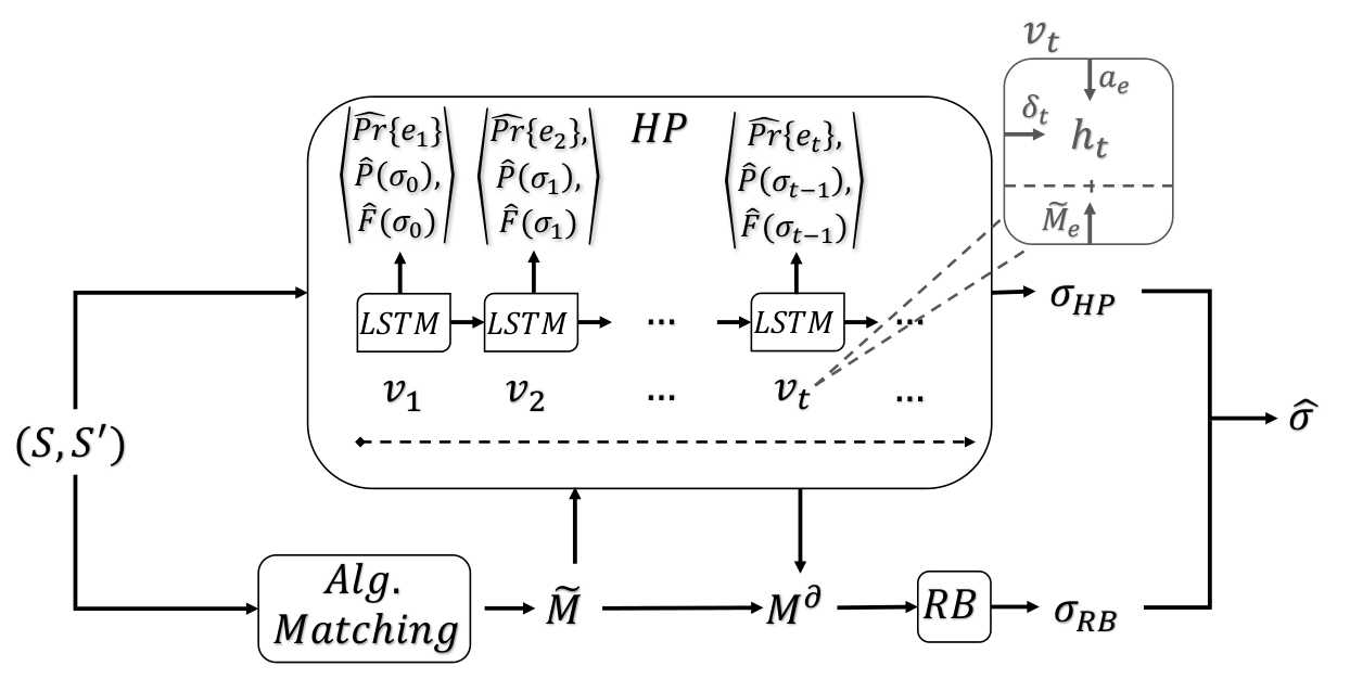
The flow of PoWareMatch is illustrated in Figure 6. Its input is a schema pair $(S,S^{\prime})$ and a decision history $H$ (Definition 3) and its output is a match $\hat{\sigma}$. PoWareMatch is composed of two components, history processing ($HP$), aiming to calibrate matching decisions (Section 4.3) and recall boosting ($RB$), focusing on improving the low recall intrinsically obtained by human matchers (Section 4.4).

The main component of PoWareMatch calibrates matching decisions by history processing ($HP$). We recall again that the matching history (Definition 3) records matching decisions of human matchers interacting with a pair of schemata, according to the order in which they were taken. In what follows, $HP$ uses the history to process the matching decisions in the order they were assigned by the human matcher. The goal of $HP$ is to improve the estimation of $Pr\{M_{ij}\in\sigma^{*}\}$ of common (biased) matching beyond using the confidence value, which is an accurate assessment only for unbiased matching. We use $Pr\{e_{t}\}$ here as a shorthand writing for the probability of an element pair assigned at time $t$ to be correct ($Pr\{h_{t}.e\in\sigma^{*}\}$).

We first propose a feature representation of matching history decisions (Section 4.3.1) to be processed using a recurrent neural network that is trained in a supervised manner to capture latent temporal properties of the matching process. Once trained, the network predicts a set of labels $\langle\hat{Pr}\{e_{t}\},\hat{P}(\sigma_{t-1}),\hat{F}(\sigma_{t-1})\rangle$ regarding each decision $h_{t}$, which is used to generate a match $\sigma_{HP}$ (Section 4.3.2).

The $HP$ component improves on the precision of the human matcher and is limited to correspondences that were chosen by a human matcher. In what follows, the resulted match may have a low recall, simply because the decision history as provided by the human matcher did not contain enough accurate correspondences to choose from. To better cater to recall, we present next a complementary component, $RB$, to boost recall using adaptation of existing 2LMs (see Section 2.2).

$RB$ uses algorithmic match results for correspondences that were not assigned by a human matcher, formally stated as $M^{\partial}=\{\tilde{M}_{ij}|\forall h\in H,h.e\not=(a_{i},b_{j})\}$. In our experiments, we use ADnEV (Shraga et al. 2020) to produce $M^{\partial}$ (see Section 5.2.2). When a human matcher does not offer an opinion on a correspondence, it may be intentional or caused inadvertently and the two are indistinguishable. $RB$ complements human matching by analyzing all unassigned correspondences.

$RB$ is a general threshold-based 2LM, from which multiple 2LMs can be derived. Unlike traditional 2LMs, which are applied over a whole similarity matrix, $RB$ is applied to $M^{\partial}$ only, letting $HP$ handle human decisions as discussed in Section 4.3. Given a partial matrix $M^{\partial}$ and a set of thresholds $\nu=\{\nu_{ij}\}$, $RB$ is defined as follows:

$RB$ forms a natural implementation of Threshold (Do and Rahm 2002) by defining $\nu^{th}$ to assign a single threshold value to all entries such that $\nu_{i,j}=\nu^{th}$ for all matrix entries $(i,j)$. To adapt Max-Delta to work with $M^{\partial}$, we separate the decision-making process by cases. Let $M_{ij}$ be the entry under consideration. In the case that a human matcher did not choose any value in row $i$, $RB$ adds $M_{ij}$ to $\sigma_{RB}$ if $M_{ij}>0$. There are two possible scenarios when a human matcher chose an entry in row $i$. If none of the entries a human matcher chose in row $i$ are included in $\sigma_{HP}$, then we are back to the first case, adding $M_{ij}$ to $\sigma_{RB}$ if $M_{ij}>0$. Otherwise, some entry in row $i$ has been included in $\sigma_{HP}$ and by using a hyper-parameter $\theta$,⁶⁶ 6 we use $\theta$ here to avoid confusion with a $\delta$ function notation. $M_{ij}$ is added to $\sigma_{RB}$ if it satisfies the Max-Delta revised condition: $M_{ij}>1-\theta$.

In what follows, each threshold in the set $\nu^{md}(\theta)$ is formally defined as follows:⁷⁷ 7 $\varepsilon\sim 0$ is a very small number assuring a strict inequality.

A straightforward variation of Max-Delta can be derived by looking at the columns instead of the rows of each entry, as initially suggested by Do et al. (Do and Rahm 2002).

The implementation of such variant of Eq. 5 is given by

Finally, we offer an extension to the original implementation of Dominants by introducing a tuning window (distance from maximal value) similar to the one defined for Max-Delta. The inference is similar to the one applied for $\nu^{md}(\theta)$ and each threshold in the set $\nu^{dom}(\theta)$ can be defined as follows:

References

- (1)
- dat (2021) 2021. Data. https://github.com/shraga89/PoWareMatch/tree/master/DataFiles.
- gra (2021) 2021. Graphs. https://github.com/shraga89/PoWareMatch/tree/master/Eval_graphs.
- oae (2021) 2021. OAEI benchmark. http://oaei.ontologymatching.org/2011/benchmarks/.
- ore (2021) 2021. Ontobuilder research environment. https://github.com/shraga89/Ontobuilder-Research-Environment.
- git (2021a) 2021a. PoWareMatch Configuration. https://github.com/shraga89/PoWareMatch/blob/master/RunFiles/config.py.
- git (2021b) 2021b. PoWareMatch repository. https://github.com/shraga89/PoWareMatch.
- tor (2021) 2021. PyTorch. https://pytorch.org/.
- tec (2021) 2021. Technical Report. https://github.com/shraga89/PoWareMatch/blob/master/PoWareMatch_Tech.pdf.
- Ackerman et al. (2019) Rakefet Ackerman, Avigdor Gal, Tomer Sagi, and Roee Shraga. 2019. A Cognitive Model of Human Bias in Matching. In Pacific Rim International Conference on Artificial Intelligence. Springer, 632–646.
- Ackerman and Thompson (2017) Rakefet. Ackerman and Valerie Thompson. 2017. Meta-Reasoning: Monitoring and control of thinking and reasoning. Trends in Cognitive Sciences 21, 8 (2017), 607–617.
- Barsalou (2014) Lawrence W Barsalou. 2014. Cognitive psychology: An overview for cognitive scientists. Psychology Press.
- Bellahsene et al. (2011b) Zohra Bellahsene, Angela Bonifati, Fabien Duchateau, and Yannis Velegrakis. 2011b. On Evaluating Schema Matching and Mapping. In Schema Matching and Mapping. Springer Berlin Heidelberg, 253–291.
- Bellahsene et al. (2011a) Zohra Bellahsene, Angela Bonifati, and Erhard Rahm (Eds.). 2011a. Schema Matching and Mapping. Springer.
- Benesty et al. (2009) Jacob Benesty, Jingdong Chen, Yiteng Huang, and Israel Cohen. 2009. Pearson correlation coefficient. In Noise reduction in speech processing. Springer, 1–4.
- Bernstein et al. (2011) Philip A. Bernstein, Jayant Madhavan, and Erhard Rahm. 2011. Generic Schema Matching, Ten Years Later. PVLDB 4, 11 (2011), 695–701.
- Bjork et al. (2013) Robert A Bjork, John Dunlosky, and Nate Kornell. 2013. Self-regulated learning: Beliefs, techniques, and illusions. Annual Review of Psychology 64 (2013), 417–444.
- Bozovic and Vassalos (2015) Nikolaos Bozovic and Vasilis Vassalos. 2015. Two Phase User Driven Schema Matching. In Advances in Databases and Information Systems. 49–62.
- Cappuzzo et al. (2020) Riccardo Cappuzzo, Paolo Papotti, and Saravanan Thirumuruganathan. 2020. Creating embeddings of heterogeneous relational datasets for data integration tasks. In SIGMOD. 1335–1349.
- Chen et al. (2018) Chen Chen, Behzad Golshan, Alon Y Halevy, Wang-Chiew Tan, and AnHai Doan. 2018. BigGorilla: An Open-Source Ecosystem for Data Preparation and Integration. IEEE Data Eng. Bull. 41, 2 (2018), 10–22.
- Do and Rahm (2002) Hong-Hai Do and Erhard Rahm. 2002. COMA—a system for flexible combination of schema matching approaches. In VLDB’02: Proceedings of the 28th International Conference on Very Large Databases. Elsevier, 610–621.
- Dong et al. (2009) Xin Dong, Alon Halevy, and Cong Yu. 2009. Data integration with uncertainty. The VLDB Journal 18 (2009), 469–500.
- Dragisic et al. (2016) Zlatan Dragisic, Valentina Ivanova, Patrick Lambrix, Daniel Faria, Ernesto Jiménez-Ruiz, and Catia Pesquita. 2016. User validation in ontology alignment. In International Semantic Web Conference. Springer, 200–217.
- Ebraheem et al. (2018) Muhammad Ebraheem, Saravanan Thirumuruganathan, Shafiq Joty, Mourad Ouzzani, and Nan Tang. 2018. Distributed Representations of Tuples for Entity Resolution. PVLDB 11, 11 (2018).
- Euzenat et al. (2007) Jérôme Euzenat, Pavel Shvaiko, et al. 2007. Ontology matching. Vol. 18. Springer.
- Falconer and Storey (2007) Sean M. Falconer and Margaret-Anne D. Storey. 2007. A Cognitive Support Framework for Ontology Mapping. In International Semantic Web Conference, ISWC. Lecture Notes in Computer Science, Vol. 4825. Springer Berlin Heidelberg, 114–127.
- Fan et al. (2014) Ju Fan, Meiyu Lu, Beng Chin Ooi, Wang-Chiew Tan, and Meihui Zhang. 2014. A hybrid machine-crowdsourcing system for matching web tables. In 2014 IEEE 30th International Conference on Data Engineering. IEEE, 976–987.
- Fernandez et al. (2018) Raul Castro Fernandez, Essam Mansour, Abdulhakim A Qahtan, Ahmed Elmagarmid, Ihab Ilyas, Samuel Madden, Mourad Ouzzani, Michael Stonebraker, and Nan Tang. 2018. Seeping semantics: Linking datasets using word embeddings for data discovery. In 2018 IEEE 34th International Conference on Data Engineering (ICDE). IEEE, 989–1000.
- Gal (2011) Avigdor Gal. 2011. Uncertain Schema Matching. Morgan & Claypool Publishers.
- Gal et al. (2019) Avigdor Gal, Haggai Roitman, and Roee Shraga. 2019. Learning to Rerank Schema Matches. IEEE Transactions on Knowledge and Data Engineering (TKDE) (2019).
- Gawinecki (2009) Maciej Gawinecki. 2009. Abbreviation expansion in lexical annotation of schema. Camogli (Genova), Italy June 25th, 2009 Co-located with SEBD (2009), 61.
- Gers et al. (2000) Felix A Gers, Jürgen Schmidhuber, and Fred Cummins. 2000. Learning to forget: Continual prediction with LSTM. Neural computation 12, 10 (2000), 2451–2471.
- Halevy and Madhavan (2003) Alon Y Halevy and Jayant Madhavan. 2003. Corpus-based knowledge representation. In IJCAI, Vol. 3. 1567–1572.
- Hammer et al. (2005) Joachim Hammer, Michael Stonebraker, and Oguzhan Topsakal. 2005. THALIA: Test Harness for the Assessment of Legacy Information Integration Approaches. In ICDE. 485–486.
- He and Chang (2005) Bin He and Kevin Chen-Chuan Chang. 2005. Making holistic schema matching robust: an ensemble approach. In Proceedings of the eleventh ACM SIGKDD international conference on Knowledge discovery in data mining. 429–438.
- Kendall (1938) Maurice G Kendall. 1938. A new measure of rank correlation. Biometrika 30, 1/2 (1938), 81–93.
- Kolyvakis et al. (2018) Prodromos Kolyvakis, Alexandros Kalousis, and Dimitris Kiritsis. 2018. Deepalignment: Unsupervised ontology matching with refined word vectors. In Proceedings of the 2018 Conference of the North American Chapter of the Association for Computational Linguistics: Human Language Technologies, Volume 1 (Long Papers). 787–798.
- Lambrix and Edberg (2003) Patrick Lambrix and Anna Edberg. 2003. Evaluation of Ontology Merging Tools in Bioinformatics. In Proceedings of the 8th Pacific Symposium on Biocomputing, PSB 2003, Lihue, Hawaii, USA, January 3-7, 2003, Vol. 8. 589–600.
- LeCun et al. (2015) Yann LeCun, Yoshua Bengio, and Geoffrey Hinton. 2015. Deep learning. nature 521, 7553 (2015), 436.
- Li (2017) Guoliang Li. 2017. Human-in-the-loop data integration. Proceedings of the VLDB Endowment 10, 12 (2017), 2006–2017.
- Li et al. (2019) Huanyu Li, Zlatan Dragisic, Daniel Faria, Valentina Ivanova, Ernesto Jiménez-Ruiz, Patrick Lambrix, and Catia Pesquita. 2019. User validation in ontology alignment: functional assessment and impact. The Knowledge Engineering Review 34 (2019).
- Li et al. (2021) Yuliang Li, Jinfeng Li, Yoshihiko Suhara, Jin Wang, Wataru Hirota, and Wang-Chiew Tan. 2021. Deep Entity Matching: Challenges and Opportunities. Journal of Data and Information Quality (JDIQ) 13, 1 (2021), 1–17.
- McCann et al. (2008) Robert McCann, Warren Shen, and AnHai Doan. 2008. Matching schemas in online communities: A web 2.0 approach. In 2008 IEEE 24th international conference on data engineering. IEEE, 110–119.
- Melnik et al. (2002) Sergey Melnik, Hector Garcia-Molina, and Erhard Rahm. 2002. Similarity flooding: A versatile graph matching algorithm and its application to schema matching. In ICDE. IEEE, 117–128.
- Metcalfe and Finn (2008) Janet Metcalfe and Bridgid Finn. 2008. Evidence that judgments of learning are causally related to study choice. Psychonomic Bulletin & Review 15, 1 (2008), 174–179.
- Modica et al. (2001) Giovanni Modica, Avigdor Gal, and Hasan M Jamil. 2001. The use of machine-generated ontologies in dynamic information seeking. In International Conference on Cooperative Information Systems. Springer, 433–447.
- Mudgal et al. (2018) Sidharth Mudgal, Han Li, Theodoros Rekatsinas, AnHai Doan, Youngchoon Park, Ganesh Krishnan, Rohit Deep, Esteban Arcaute, and Vijay Raghavendra. 2018. Deep Learning for Entity Matching: A Design Space Exploration. In Proceedings of the 2018 International Conference on Management of Data. ACM, 19–34.
- Nguyen et al. (2014) Quoc Viet Hung Nguyen, Thanh Tam Nguyen, Zoltán Miklós, Karl Aberer, Avigdor Gal, and Matthias Weidlich. 2014. Pay-as-you-go reconciliation in schema matching networks. In ICDE. IEEE, 220–231.
- Noy et al. (2013) Natalya Fridman Noy, Jonathan Mortensen, Mark A. Musen, and Paul R. Alexander. 2013. Mechanical turk as an ontology engineer?: using microtasks as a component of an ontology-engineering workflow. In Web Science 2013, WebSci ’13. 262–271.
- Noy and Musen (2002) Natalya F Noy and Mark A Musen. 2002. Evaluating ontology-mapping tools: Requirements and experience. In Workshop on Evaluation of Ontology Tools at EKAW, Vol. 2. p1–14.
- Peukert et al. (2011) Eric Peukert, Julian Eberius, and Erhard Rahm. 2011. AMC-A framework for modelling and comparing matching systems as matching processes. In 2011 IEEE 27th International Conference on Data Engineering. IEEE, 1304–1307.
- Pinkel et al. (2013) Christoph Pinkel, Carsten Binnig, Evgeny Kharlamov, and Peter Haase. 2013. IncMap: pay as you go matching of relational schemata to OWL ontologies.. In OM. Citeseer, 37–48.
- Rahm and Bernstein (2001) Erhard Rahm and Philip A Bernstein. 2001. A survey of approaches to automatic schema matching. the VLDB Journal 10, 4 (2001), 334–350.
- Ross et al. (2010) Joel Ross, Lilly Irani, M Silberman, Andrew Zaldivar, and Bill Tomlinson. 2010. Who are the crowdworkers?: shifting demographics in mechanical turk. In CHI’10 Extended Abstracts on Human Factors in Computing Systems. ACM, 2863–2872.
- Sarasua et al. (2012) C. Sarasua, E. Simperl, and N. F Noy. 2012. Crowdmap: Crowdsourcing ontology alignment with microtasks. In ISWC.
- Shraga et al. (2018) Roee Shraga, Avigdor Gal, and Haggai Roitman. 2018. What Type of a Matcher Are You?: Coordination of Human and Algorithmic Matchers. In Proceedings of the Workshop on Human-In-the-Loop Data Analytics, HILDA@SIGMOD. 12:1–12:7.
- Shraga et al. (2020) Roee Shraga, Avigdor Gal, and Haggai Roitman. 2020. ADnEV: Cross-Domain Schema Matching using Deep Similarity Matrix Adjustment and Evaluation. Proceedings of the VLDB Endowment 13, 9 (2020), 1401–1415.
- Singh et al. (2017) Rohit Singh, Venkata Vamsikrishna Meduri, Ahmed Elmagarmid, Samuel Madden, Paolo Papotti, Jorge-Arnulfo Quiané-Ruiz, Armando Solar-Lezama, and Nan Tang. 2017. Synthesizing entity matching rules by examples. Proceedings of the VLDB Endowment 11, 2 (2017), 189–202.
- Thirumuruganathan et al. (2020) Saravanan Thirumuruganathan, Nan Tang, Mourad Ouzzani, and AnHai Doan. 2020. Data Curation with Deep Learning. In EDBT. 277–286.
- Wang et al. (2019) Pei Wang, Ryan Shea, Jiannan Wang, and Eugene Wu. 2019. Progressive Deep Web Crawling Through Keyword Queries For Data Enrichment. In Proceedings of the 2019 International Conference on Management of Data. 229–246.
- Willmott and Matsuura (2005) Cort J Willmott and Kenji Matsuura. 2005. Advantages of the mean absolute error (MAE) over the root mean square error (RMSE) in assessing average model performance. Climate research 30, 1 (2005), 79–82.
- Zhang et al. (2018) Chen Zhang, Lei Chen, HV Jagadish, Mengchen Zhang, and Yongxin Tong. 2018. Reducing Uncertainty of Schema Matching via Crowdsourcing with Accuracy Rates. IEEE Transactions on Knowledge and Data Engineering (2018).
- Zhang et al. (2013) Chen Jason Zhang, Lei Chen, H. V. Jagadish, and Caleb Chen Cao. 2013. Reducing Uncertainty of Schema Matching via Crowdsourcing. PVLDB 6, 9 (2013), 757–768.
- Zhang and Ives (2020) Yi Zhang and Zachary G Ives. 2020. Finding Related Tables in Data Lakes for Interactive Data Science. In Proceedings of the 2020 ACM SIGMOD International Conference on Management of Data. 1951–1966.
Appendix A Monotonic Evaluation and Section 3 Proofs
The appendix is devoted to the proofs of Section 3.
Theorem 1.
Recall () is a MIEM over , Precision () is a MIEM over , and f-measure () is a MIEM over .
For proving Theorem 2, we use two lemmas stating that recall is a MIEM over all match pairs in and, since precision and f-measure are not monotonic over the full set of pairs in , the conditions under which monotonicity can be guaranteed for both measures.
Lemma 0.
Recall () is a MIEM over .
Proof of Lemma 2.
Let be a match pair in . Using Eq. 1, one can compute recall of and , as follows.
and thus and . Noting that the denominator is not affected by the addition, we obtain:
and thus . ∎
For :
- •
iff
Proof of Lemma 3.
Let be a match pair in . We shall begin with two extreme cases in which the denominator of a precision calculation is zero. First, in case , is undefined. Accordingly, for this work, we shall define , i.e., the prior precision value does not change. Second, in the case , we obtain that resulting in an undefined . Similarly, we define , i.e., expanding a match with nothing does not “harm” its precision. In both cases we obtain and the first statement of the lemma holds.
Next, we refer to the general case where and and note that . Assuming and recalling that (), we obtain that and