Patient-specific solution of the electrocorticography
forward problem in deforming brainJournal: NeuroImage
Abstract
Invasive intracranial electroencephalography (iEEG) or electrocorticography (ECoG) measures electric potential directly on the surface of the brain and can be used to inform treatment planning for epilepsy surgery. Combined with numerical modeling they can further improve accuracy of epilepsy surgery planning. Accurate solution of the iEEG or ECoG forward problem, which is a crucial prerequisite for solving the inverse problem in epilepsy seizure onset zone localization, requires accurate representation of the patient’s brain geometry and tissue electrical conductivity after implantation of electrodes. However, implantation of subdural grid electrodes causes the brain to deform, which invalidates preoperatively acquired image data. Moreover, postoperative magnetic resonance imaging (MRI) is incompatible with implanted electrodes and computed tomography (CT) has insufficient range of soft tissue contrast, which precludes both MRI and CT from being used to obtain the deformed postoperative geometry. In this paper, we present a biomechanics-based image warping procedure using preoperative MRI for tissue classification and postoperative CT for locating implanted electrodes to perform non-rigid registration of the preoperative image data to the postoperative configuration. We solve the iEEG forward problem on the predicted postoperative geometry using the finite element method (FEM) which accounts for patient-specific inhomogeneity and anisotropy of tissue conductivity. Results for the simulation of a current source in the brain show large differences in electric potential predicted by the models based on the original images and the deformed images corresponding to the brain geometry deformed by placement of invasive electrodes. Computation of the lead field matrix (useful for solution of the iEEG inverse problem) also showed significant differences between the different models. The results suggest that rapid and accurate solution of the forward problem in a deformed brain for a given patient is achievable.
Keywords:
epilepsy, electroencephalography, biomechanics, diffusion tensor imaging, meshless methods, finite element method (FEM)Introduction
Techniques to construct patient-specific models of brain bioelectric activity, and to solve such models accurately and efficiently, form a key enabling technology for neuroscience and neurology (Baillet et al. 2001; Brette and Destexhe 2012). Of particular interest is the application of such modeling and simulation techniques to identification of epileptic seizure onset zones (SOZ) which consider the brain at length scales accessible by noninvasive neuroimaging (such as CT, US and MRI), and scalp electrodes, subdural electrode grids and strips, or depth electrodes (Baillet et al. 2001; Brette and Destexhe 2012). The spatial resolution of medical images such as MRI and CT, and dimensions of scalp EEG and subdural ECoG electrodes—as well as the accuracy of surgery—are on the order of 1 mm, but in current practice the SOZ is usually located with much lower accuracy (Brodbeck et al. 2011; Michel and Brunet 2019; Mouthaan et al. 2019).
Epilepsy is a chronic brain disorder that causes unpredictable and recurrent electrical activity in the brain (seizures). Nowadays, epilepsy is treated with medication. Although drugs do not cure epilepsy, they can efficiently control seizures in up to 60% of patients. In the remaining 40%, drug therapy fails to control seizures, and surgical resection appears as a feasible alternative (Engel 2003; Engel 2018; World Health Organization 2019). However, surgical treatment of epilepsy has been the most underutilized of all proven effective therapeutic interventions in the field of medicine (Engel 2003; Engel 2018; Hader et al. 2013; Jetté and Wiebe 2015; Jobst and Cascino 2015). This is because the success of surgical resection depends on the accurate identification of the seizure onset zone (SOZ) and it is often very difficult to characterize epileptic activity of the brain and identify appropriate resection regions with sufficient accuracy to proceed with surgery.
The SOZ is often identified with the help of intracranial measurement of electric potential during a seizure. An intracranial electroencephalogram (iEEG) or electrocorticography (ECoG) (Jayakar et al. 2016) records electrical activity from the cerebral cortex using electrodes placed directly on the exposed surface of the brain (Fig. 1a), whereas stereoelectroencephalography (SEEG) (Minotti et al. 2018) enables exploration of deeply located structures using needle-like depth electrodes inserted inside the brain (Fig. 1b). Implantation of electrodes is an invasive procedure and therefore applied rarely, as the measurements by these electrodes do not directly yield the location of the seizure onset zone with accuracy comparable to imaging resolutions, but rather form an input to further analysis. Source modeling is one way to process that information and combine it with other imaging information and prior assumptions. To increase the utilization of epilepsy surgery there is a pressing need for new and more effective methods of SOZ localization that will enable clinicians to cure epilepsy in a greater number of patients. As it is estimated that 20 million people globally have focal epilepsy that can be permanently cured by precisely targeted surgery (World Health Organization 2019), methods for successful identification of the SOZ would be of enormous health benefit. One such promising technology is source localization from invasive measurements. Using a volume conductor model of a patient’s head as the basis for an inverse problem, source localization maps individual electrode measurements to three dimensional maps of distribution of electric potential within the brain. These maps have the potential to significantly improve SOZ identification by improved analysis of invasive EEG data.

Accurate and robust patient-specific models of brain bioelectric activity could have applications well beyond guiding surgical treatment of epilepsy. These include the analysis of extracranial measurement data, such as standard electroencephalogram (EEG) and magnetoencephalogram (MEG) often used in neurology, neuroscience and neuropsychiatry (Brette and Destexhe 2012), as well as generation of high-quality synthetic training data for artificial intelligence (AI) systems based on neural networks. This last possible application is becoming particularly important, as in recent years, deep learning has started to gain popularity for bioelectric signal processing (Cendes and McDonald 2022; Liu et al. 2021; Sun and Sclabassi 2000; Tobore et al. 2019). With a large amount of data, it outperforms traditional feature extraction in terms of classification accuracy (Hu et al. 2019). Deep learning algorithms, especially the convolutional neural network (CNN), are also gradually being adopted in epilepsy management, for example for seizure detection (Gao et al. 2020; Thomas et al. 2018).
Source localization based on ECoG or iEEG can be split into two separate problems: the forward problem that involves calculating the electric potential within the brain volume given a predefined source (or multiple sources); and the inverse problem that involves finding the source location (or locations) given electric potential measurements at the sensor electrodes (Baillet et al. 2001; Brette and Destexhe 2012; Hallez et al. 2007; Grech et al. 2008). In addition to considerations specific to the inverse problem, such as selection of the number of sources and the choice of source localization algorithms (Bradley et al. 2016; Grech et al. 2008; Scherg et al. 2019), source localization requires an accurate solution of the iEEG forward problem, which depends on an accurate representation of the geometry of the patient’s brain and electrical conductivity distribution within the patients head (Brette and Destexhe 2012; Hallez et al. 2007; Vorwerk et al. 2014; Wolters et al. 2006).
This study is based on the realization that a patient’s brain is significantly deformed by the implantation of the electrodes (Fig. 1). The shift in the brain surface caused by implantation of ECoG grid electrodes is typically on the order of around 5 mm, but often exceeds 10 mm (Foldes et al. 2020; Hill et al. 2000). Consequently, models built from preoperative images that do not account for this brain shift will be geometrically very inaccurate. To remedy this situation, we demonstrate how to construct a volume conductor model corresponding to the true deformed brain geometry and how to solve quickly the iEEG forward problem—a prerequisite for the iEEG inverse problem that ultimately needs to be solved to localize sources.
In some previous studies, to account for craniotomy-induced brain shift during placement of grid electrodes, the electrode positions identified from the postoperative CT were projected onto the cortical surface extracted from the preoperative MRI (Dykstra et al. 2012; Yang et al. 2012; Tao et al. 2009; LaViolette et al. 2011; Hermes et al. 2010; Taimouri et al. 2014). Although this approach solves the issue of the electrodes being erroneously located within the brain tissue instead of on the surface of the brain, it does not accurately reflect the actual postoperative configuration of the brain. In the current study, instead of projecting the electrode positions onto the undeformed preoperative cortical surface, we aim to predict the postoperative configuration of the brain such that the cortical surface of the model used for solving the iEEG forward problem corresponds to the actual position of the implanted surface electrode array.
In this paper, we propose a novel modeling pipeline for iEEG source localization that incorporates the tissue deformation caused by the craniotomy and placement of the electrodes. Using preoperative MR and postoperative CT images, our approach employs biomechanics-based image warping to predict the postoperative configuration of the brain (i.e. the configuration deformed by the implantation of intracranial electrodes). The postoperative CT is used to locate the electrode positions and to inform the boundary conditions and loading of the biomechanical model. The approach taken in this study is to register the preoperative anatomical MRI and DTI onto the postoperative CT (with electrodes implanted) using a displacement field computed by a biomechanical model (Miller et al. 2019a; Mostayed et al. 2013; Safdar et al. 2021; Wittek et al. 2007; Wittek and Miller 2020; Yu et al. 2022) to obtain warped MRI and DTI corresponding to the postoperative, deformed configuration of the patient’s brain. Based on these warped images we construct a geometrically correct computational domain on which the partial differential equations of the iEEG forward problem are solved, as well as inhomogeneous and anisotropic patient-specific distribution of conductivity tensor used in the solution procedure.
Continuum models based on partial differential equations are the dominant method for brain bioelectric activity modeling at the spatial and temporal scales accessible via ECoG, iEEG, EEG or MEG. Numerical solution of these equations have attracted considerable attention in the literature. Mainstream numerical methods, such as finite element (FEM) (Drechsler et al. 2009; Marin et al. 1998; Medani et al. 2021; Pursiainen et al. 2011; Schimpf et al. 2002; Schrader et al. 2021), finite volume (FVM) (Cook and Koles 2006), finite difference (FDM) (Bourantas et al. 2020; Hyde et al. 2012; Saleheen and Ng 1997; Wendel et al. 2008) and boundary element methods (BEM) (Acar and Makeig 2010; Meijs et al. 1989; Stenroos and Sarvas 2012), as well as newer, more sophisticated methods such as meshless methods (Fiétier et al. 2013) that use a point cloud to represent the spatial domain, have been used to numerically solve the governing equations of the EEG forward problem.
The finite element method (FEM) achieves high numerical accuracy (Drechsler et al. 2009; Vorwerk et al. 2012; Vorwerk et al. 2018) and can be easily used to model complex geometries having anisotropic conductivities (Gullmar et al. 2006; Güllmar et al. 2010; Haueisen et al. 2002; Rullmann et al. 2009; Vorwerk et al. 2014; Wolters et al. 2006). The FEM uses a tessellation of the computational domain in which the domain is partitioned into a set of elements of simple shape, such as tetrahedrons or hexahedrons. Tetrahedral meshes are generated by constrained Delaunay tetrahedralization from segmented and reconstructed tissue surface representations (Vorwerk et al. 2014). On the other hand, regular hexahedral meshes can be easily generated from voxel-based raw image data (Schimpf et al. 2002; Rullmann et al. 2009; Vorwerk et al. 2017). This greatly simplifies mesh generation which is an important consideration for ensuring compatibility with clinical workflows. Moreover, regular hexahedra have favourable numerical properties over skewed hexahedra or tetrahedra (Hughes 2000), Geometry-adapted hexahedra (Wolters et al. 2007a) or tetrahedra (Vorwerk et al. 2017) may give similar results using less elements but this comes at the significant cost of additional complications of mesh generation.
Our methodology is an embodiment of the “image-as-a-model” concept (Zhang et al. 2013) as it is entirely voxel-based and the finite element method with a mesh coinciding with the voxelized structure of the image is used to obtain the solution. The advantage of this voxel-based analysis includes straight-forward generation of realistic patient-specific models from three-dimensional image data and a simple data structure that is suitable for storage, handling, numerical solution and visualization (Rullmann et al. 2009; Schimpf et al. 1998; Schimpf et al. 2002).
To demonstrate the application of the proposed methodology and to quantify the effect of geometric accuracy on the model solutions, we solve two example problems using the original preoperative geometry (with both the actual and projected electrode positions) and the geometry after model based image deformation. In the first example, we apply a current dipole inside the brain and compare the potential computed at the electrodes. In the second example, we compute the lead field matrices (gain matrices relating the source space with the measurement space which are often used in the solution of the EEG inverse problem) using the models constructed from the original and deformed image data, and compare the difference between the two sets of results. In both examples, the large difference in the results obtained using the original and deformed image data suggest that the forward problem solution accuracy may be improved by accounting for electrode-induced brain shift in the patient-specific volume conductor model as described herein, which, when combined with suitable inverse solution methods, may lead to improved accuracy in source localization.
The paper is organized as follows. In section 2, we describe the mathematical model, patient-specific model construction and the components of the numerical methodology. In section 3, we provide patient-specific numerical results confirming robustness and efficiency of our modeling and simulation pipeline, as well as demonstrating inaccuracies of using models built directly from preoperative, undeformed images. Section 4 contains discussion and conclusions.
Methods
Governing equations of the brain bioelectric activity at scales as measured by EEG and MRI
The electroencephalography (EEG) forward problem involves predicting the electric potential within the brain and at the implanted electrodes given a predefined source. The relevant frequency spectrum in EEG is typically below 1 kHz, with most studies dealing with frequencies between 0.1 and 100 Hz (Baillet et al. 2001; Brette and Destexhe 2012). Therefore, the physics of EEG can be approximated by Poisson’s equation, which is the quasi-static approximation of Maxwell’s equations. For a spatial domain with boundary and outward unit normal , Poisson’s equation for the EEG forward problem can be written as follows:
| (1) | ||||
| (2) | ||||
| (3) |
where is the unknown scalar potential and is the (symmetric positive semi-definite) conductivity tensor. The low conductivity of air outside the scalp ( for all ) implies that a zero-flux Neumann boundary condition can be applied on the surface . Dirichlet boundary conditions on the surface are typically applied by setting the potential to zero at a node corresponding to a reference electrode. Loading can be applied to the model either by prescribing the potential at certain nodes or by applying a current source , with being a dipole source vector. The epileptic seizure onset source is typically modeled as a current dipole (Hallez et al. 2007).
Electromagnetic source localization employs a linear model, known as the lead field matrix, which relates the measured electrode voltages to the cerebral current sources that generated them (Rush and Driscoll 1969; Weinstein et al. 2000). The lead field matrix can be computed using Helmholtz’s principle of reciprocity, which relates the potential difference between two points and caused by a given dipole , to the electric field at the dipole location resulting from a current placed between and (Plonsey 1963; Weinstein et al. 2000):
| (4) |
The lead field matrix can be constructed by placing a source and sink at pairs of electrodes, and computing for each of these pairs the resulting electric field in all of the elements. The reciprocity principle can then be applied to reconstruct the potential differences at the electrodes for a source placed in any element (Weinstein et al. 2000).
Computation of the lead field matrix requires the solution of the forward problem for each sensor and ground electrode pair. To compute the lead field matrix, one electrode is selected arbitrarily as the ground (or reference) electrode. For each lead field (row in the lead field matrix), a unit current is applied to one of the sensor (non-ground) electrodes. The electric field in each element is computed as the gradient of the electric potential and represents a row in the matrix. The potential at the non-ground electrodes for a source located in any of the elements is given by
| (5) |
where , of dimension , is the lead field matrix, and , of dimension , is a vector of dipole amplitudes in all points of the source space.
Patient-specific model generation
In this section, we describe the methods used to create a detailed patient-specific model for the EEG forward problem. Accurate solution of the EEG forward problem requires a correspondingly accurate representation of both the computational domain ( in Eq. (1)) and the tissue conductivity ( in Eq. (1)) throughout the conducting head volume. The head volume is bounded by the rigid skull and scalp which can be easily extracted from the preoperative images. The brain, however, is a soft tissue that deforms due to the insertion of the electrode grid array. To take into account the brain shift following electrode insertion we apply our biomechanics-based image warping techniques to predict the postoperative brain geometry. Fig. 2 provides a flowchart of the proposed methodology.
A detailed description of each step is provided in the following subsections.
We created the following three models for comparison of the different modeling approaches:
- 1.
unwarped model based on preoperative (unwarped) image data with actual electrode positions identified from postoperative CT;
- 2.
projected model based on preoperative (unwarped) image data with electrode positions projected from their actual locations identified from postoperative CT onto the cortical surface; and
- 3.
warped model based on postoperative (warped) image data predicted by biomechanics-based image registration with actual electrode positions identified from postoperative CT.
Image acquisition and image processing
To create the patient-specific EEG forward model we require preoperative anatomical magnetic resonance image (MRI) to obtain the undeformed brain geometry; preoperative diffusion tensor image (DTI) to classify tissue types at each voxel and to estimate patient-specific tissue conductivity; and postoperative computed tomography (CT) to locate the implanted electrodes.
T1 and T2 weighted structural MRI scans and diffusion MRI were collected from a 12 year old female epilepsy patient under evaluation for surgical intervention at Boston Children’s Hospital (BCH ethics approval no. IRB-P00025254, UWA ethics approval no. RA/4/1/9336). The T1w MPRAGE image was acquired in the saggital plane at a nominal resolution of mm (21 cm FOV, inplane matrix size of and 160 slices). The T2w TSE MRI was acquired at nominal resolution of mm. The DWI acquisition was at a nominal resolution of mm. All images were coregistered to the T1 scan using a rigid transformation, estimated by optimizing the mutual information between the two images (Grau et al. 2004; Weisenfeld and Warfield 2009) as implemented in CRKIT (http://crl.med.harvard.edu/software), and resampled to have matching 1 mm isotropic resolution. Residual distortion and patient motion in the DWI was compensated for by alignment to the T1w MPRAGE and appropriate reorientation of gradient directions (Peters et al. 2012; Ruiz-Alzola et al. 2002). Diffusion tensors were estimated using robust least squares. The dimensions of the images are voxels with spacing (Fig. 3).
An grid of platinum-iridium electrode disks (4 mm diameter, 10 mm spacing) embedded in a non-conductive silastic substrate (2 mm thickness) was placed on the cortical surface through a craniotomy. Electrode placements were identified from postoperative CT, coregistered and resampled to the resolution of the preoperative MRI. Intensity thresholding was used to identify individual electrodes, with manual validation of electrode separation.
The postoperative electrode positions were projected onto the preoperative brain surface to obtain the displacement of the brain surface in the vicinity of the electrodes that is used to define loading in the biomechanical model (see section 2.2.2), and to correct for the intraoperative brain shift in the model that was based on undeformed preoperative image data with projected electrode positions (Taimouri et al. 2014). We used the ImplicitPolyDataDistance method of the Visualization Toolkit (Schroeder et al. 2006) to compute the distance from each electrode as seen on CT to the corresponding nearest point on the undeformed brain surface mesh.

Patient-specific geometry
Brain deformation due to intracranial electrode array insertion
Insertion of intracranial electrodes results in significant brain deformations that need to be accounted for when defining the domain on which the EEG forward problem needs to be solved. The deformed (with respect to the original preoperative MRI and DTI) postoperative configuration of the brain was obtained using biomechanics-based image warping (Miller et al. 2019a). In this approach, the brain tissue is modeled as a deformable solid and the displacement field is computed using a meshless total Lagrangian explicit dynamics algorithm (Joldes et al. 2019). The methodology used to compute the brain shift, caused in this study by the implantation of electrodes, has been extensively validated in our previous studies (Garlapati et al. 2014; Ma et al. 2011; Miller et al. 2011; Miller et al. 2019b; Mostayed et al. 2013; Wittek et al. 2007; Wittek et al. 2010; Wittek and Miller 2020).
The computational grid for the biomechanical model was created as follows. We applied the skull stripping procedure available in FreeSurfer (http://surfer.nmr.mgh.harvard.edu) (Dale et al. 1999), an open-source software suite for processing and analyzing human brain MRIs, to the preoperative T1-weighted anatomical MRI to create a brain mask (i.e., a binary label map that is nonzero in the region of the brain only). The triangulated surface of the brain mask segment was extracted and remeshed using PyACVD (https://github.com/pyvista/pyacvd) to obtain a high quality uniformly refined surface mesh. A tetrahedral grid was generated from the surface mesh of the brain using Gmsh (https://gmsh.info) (Geuzaine and Remacle 2009). The vertices of this grid were used as nodes for the meshless approximation of the variable of interest (displacement), while the tetrahedral cells were used for numerical integration of the weak form. The meshless biomechanical model contained 18,434 nodes (includes rigid skull nodes), 44,821 tetrahedral integration cells, and 179,284 integration points. Note that the computational methods and grid used to solve the biomechanical model as described in this section are different to those used for the EEG forward problem, which is solved using the finite element method with a regular hexahedral grid as described in section 2.3.
The mechanical response of brain tissue was modeled using a modified neo-Hookean constitutive equation with strain energy density (Zienkiewicz et al. 2013)
| (6) |
where is the determinant of the deformation gradient and is the first invariant of the right Cauchy-Green deformation tensor. The shear modulus, , and Lamé’s first parameter, , are related to the Young’s modulus, , and Poisson’s ratio, , by the following relationships:
| (7) |
The material parameters and were assigned to each voxel using fuzzy tissue classification (Li et al. 2016; Zhang et al. 2013) conducted on preoperative MRI. As in our previous work (Wittek et al. 2010; Miller et al. 2019a), we used Pa and for brain tissue, and Pa and for cerebrospinal fluid.
As the brain deformations are caused by electrode array insertion, the loading is defined based on the displacement between the brain surface of the preoperative MRI and the location of electrodes in the postoperative CT, rigidly registered to preoperative MRI. The displacement magnitude at each node was obtained by first projecting the electrode centroids from the postoperative CT onto the preoperative brain surface. The displacements of the grid nodes were obtained by interpolating the displacements from the electrode centroids using moving least squares (MLS) approximation (Lancaster and Salkauskas 1981). The maximum displacement applied was 21.9 mm. The brain deformation problem with displacement loading is a Dirichlet-type problem and therefore the computed displacements are only weakly sensitive to the assumed material model (Wittek et al. 2009; Ma et al. 2011; Miller and Lu 2013).
The skull was modeled as a rigid surface approximated by the outer surface of the brain mask. Contact between the brain and the skull was modeled using a frictionless finite sliding contact algorithm (Joldes et al. 2008).
The biomechanical model was solved using the meshless total Lagrangian explicit dynamics (MTLED) algorithm (Horton et al. 2010; Miller et al. 2012; Joldes et al. 2019). The MTLED method uses modified moving least squares (MMLS) shape functions (Joldes et al. 2015) and an explicit central difference method with adaptive dynamic relaxation to obtain the static solution (Joldes et al. 2011).
Image transformations using the computed displacement field
We projected the displacement vector field onto the image grid, using the same MMLS shape functions as those used to obtain the solution of the biomechanical model, to obtain the forward displacement field transform. The forward displacement field transform maps each point to its transformed position. However, for image warping the inverse transform that maps each point to its original location is required. The forward displacement field transform was inverted using 3D Slicer (https://www.slicer.org) (Fedorov et al. 2012), allowing it to be applied directly to scalar, vector or tensor images.
The scalar images (MRIs) were transformed using the ResampleScalarVectorDWIVolume module in 3D Slicer. Fig. 4 shows the electrode positions with respect to the original and deformed image data.

The diffusion tensor image (DTI) was transformed using the ResampleDTIVolume module in 3D Slicer with linear interpolation and the preservation of the principal direction (PPD) tensor transformation method (Alexander et al. 2001). Fig. 5 shows the orientation of the diffusion tensors with respect to the original and deformed image data.

Patient-specific conductivity tensor distribution
Voxel labeling
In order to assign conductivity tensors to the image voxels we consider five tissue types in the image: skull, scalp, white matter (WM), gray matter (GM) and cerebrospinal fluid (CSF). Scalar quantities derived from the diffusion tensor, such as mean diffusivity and fractional anisotropy, can be used to classify brain tissue into CSF, GM and WM based on their diffusion properties (Pierpaoli et al. 1996). For the purpose of this study, we performed the tissue classification of the original and deformed DTIs using fuzzy C-means clustering in two steps. In the first step, we used the mean diffusivity to separate the CSF from the brain tissue. In the second step, we used the fractional anisotropy to separate the WM from the GM. The fuzziness parameter was set to . We do not generate any segmentation surfaces and we do not require that parts of the same tissue class are connected. This method of tissue classification does not require any user interaction which greatly simplifies the patient-specific model generation.
To evaluate the accuracy of our automated DTI-based tissue classification procedure we compared our segmentation results with those obtained using the STAPLE method (Warfield et al. 2004). Table 1 lists the number of voxels that belong to white matter, gray matter and CSF using the different segmentation methods. The results are very close as shown in Fig. 6.
| STAPLE | Our method | |||||
|---|---|---|---|---|---|---|
| Voxels | Volume (cm3) | Percentage | Voxels | Volume (cm3) | Percentage | |
| WM | 291,185 | 348.3 | 28.4 | 214,381 | 256.5 | 20.3 |
| GM | 660,152 | 789.7 | 64.5 | 673,756 | 806.0 | 63.7 |
| CSF | 72,434 | 86.7 | 7.1 | 169,119 | 202.3 | 16.0 |
| Total | 1,023,771 | 1224.7 | 100.0 | 1,057,256 | 1264.8 | 100.0 |
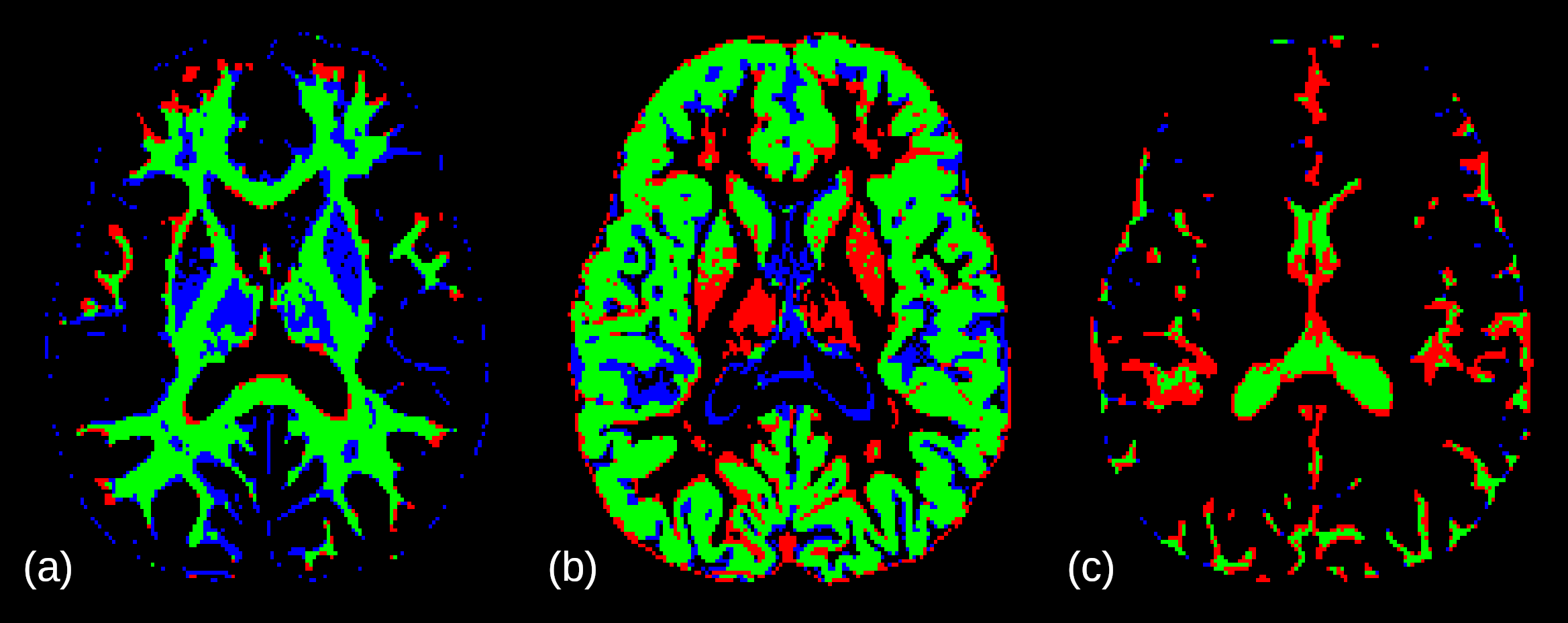
More sophisticated methods, some also based on fuzzy C-means clustering (Wen et al. 2013), may be used to improve the labeling accuracy. Segmentation using automated methods that use atlas-based approaches, however, may be difficult to apply because the postoperative configuration of the brain is often very different to a typical healthy brain. The relatively simple automated approach used here demonstrates that the method may be potentially applied in the clinic with minimal manual intervention.
Fusion of preoperative MRI and DTI, postoperative CT, and deformed MRI and DTI data
Two label maps, one based on the original preoperative MRI and the other based on the warped MRI corresponding to the postoperative configuration of the brain were created by combining the original preoperative data (skull and scalp) with the original preoperative or predicted postoperative data (original or deformed brain classified as WM, GM or CSF) and actual postoperative CT (electrode grid array). The cavity between the brain and the skull was filled with CSF. Fig 7 shows the label maps for the EEG forward models constructed using the original preoperative and deformed by electrode insertion postoperative MR images. In the preoperative image, the region between the skull and the ECoG electrodes that were placed on the brain surface is labelled as brain tissue but this clearly does not match the post-implantation situation. This indicates that using preoperative, undeformed images for patient-specific geometry generation may yield very inaccurate models.
The skull is difficult to segment from the CT image because electrodes and beam hardening artifacts pollute the image with regions of similar intensity as the skull. Many of these regions overlap with bone tissue of the skull which makes it impossible to apply simple thresholding methods to extract the bone tissue. Furthermore, fusion of the deformable soft tissue segments and the rigid but resected and non-conforming skull segment would add significant complications to the imaging pipeline. Therefore, for simplicity, we included the skull and scalp regions in the model by offsetting the brain surface by 4.4 mm (4 voxels). The effect of this simplified skull and scalp geometry on the model results should be negligible. For invasive iEEG or ECoG, as compared to non-invasive scalp EEG, the measurements are taken directly from the brain surface and attenuation by the skull is minimal which suggests that the electrical properties of the skull have little effect on the electric field within the brain (Hallez et al. 2007). Alternatively, the skull may be segmented from the CT image to provide a more realistic representation of the geometry, but this requires time consuming manual segmentation which is incompatible with a clinical workflow.
The voxels corresponding to the actual and projected locations of the electrode grid array substrate were identified by fitting a surface through the actual electrode centroids visible in the CT image and the electrode centroids projected onto the cortical surface as described in section 2.2.1. The electrode centroids were triangulated to generate a surface representing the electrode grid array substrate. This surface was refined and extruded by the equivalent distance of 2 voxels in the direction away from the brain to create a closed volume. The volume was used to create a segment representing the substrate that is at least one layer thick throughout to ensure that there was no current leakage.

Conductivity tensor assignment
The five tissue classes in the EEG forward model were assigned conductivity tensors as follows. Isotropic conductivities (Table 2) were assigned to the scalp, skull, cerebrospinal fluid (CSF), electrode grid array substrate and gray matter regions (Hallez et al. 2007; Vorwerk et al. 2014). The anisotropic conductivity of the white matter was estimated from the diffusion tensors using the fractional method with empirically defined scaling factors introduced by Tuch et al. 2001. The mean conductivity () of white matter was in the range from to 0.99 S/m,with an average value of 0.56 S/m, which agrees with values reported in the literature (Haueisen et al. 1997; Tuch et al. 2001). Fig 8 shows the mean conductivity for the model based on preoperative images and the model corresponding to the postoperative, deformed configuration of the brain. The unphysical conductivities of the brain tissue between the electrode grid array (represented by the tissue with conductivity close to zero) and the skull are clearly visible, whereas regions further from the implanted electrodes (and therefore further from the deformed brain surface) have similar conductivities in both images.
| Compartment | Conductivity (S/m) | References |
|---|---|---|
| Scalp | 0.33 | Geddes and Baker 1967; Stok 1987 |
| Skull | 0.012 | Hallez et al. 2007; Gutierrez et al. 2004 |
| Cerebrospinal fluid (CSF) | 1.79 | Baumann et al. 1997 |
| Electrode grid array | ||
| Gray matter | 0.33 | Geddes and Baker 1967; Stok 1987 |

Solution procedure for the EEG forward problem
The finite element method using a structured hexahedral mesh is an attractive choice because the mesh can be directly generated from voxel-based medical images, whereas the generation of surface-based tetrahedral meshes is more complicated (Schimpf et al. 1998; Schimpf et al. 2002; Rullmann et al. 2009; Vorwerk et al. 2017; Wolters et al. 2007a). Although geometry-adapted hexahedral and tetrahedral meshes can achieve better accuracy than regular hexahedral meshes with similar number of degrees of freedom (Wolters et al. 2007a; Vorwerk et al. 2017), it is recognized that creating patient-specific, geometry-conforming meshes is not feasible in clinical applications (Wittek et al. 2016; Vorwerk et al. 2017). The generation of a regular hexahedral mesh takes advantage of the cubic voxel structure which is inherent to medical images. This greatly simplifies mesh generation which is an important consideration for ensuring compatibility with clinical workflows. Moreover, regular hexahedra have better numerical properties than skewed hexahedra or tetrahedra (Hughes 2000). In this study, we used a regular hexahedral mesh with resolution of 1 mm, the same resolution as that used in similar previous studies (Haueisen et al. 2002; Rullmann et al. 2009; Vorwerk et al. 2017), which ensures that the CSF compartment is appropriately modeled and the skull is a closed compartment.
The conductivity tensors were assigned directly from voxels to integration points in the elements. We refer to this approach as the “image-as-a-model” concept because the finite element mesh used to solve the problem corresponds directly to the image data with one-to-one correspondence between mesh elements and image voxels. This eliminates time-consuming generation of body-fitted meshes and results in a structured hexahedral mesh with perfect element quality since all elements are cubes. The finite element mesh for the EEG forward problem contained 1,618,745 nodal points and 1,565,095 linear hexahedral elements, compared to 5,898,240 voxels in the original images (the excluded elements correspond to voxels of air outside the head).
The EEG forward problem solution method was implemented using the open-source MFEM library (Anderson et al. 2020) (https://mfem.org). A continuous Galerkin formulation with linear hexahedral elements was used for the spatial discretisation of the potential and for computing its gradient, the electric field. The finite element method is based on the weak form of the governing equations which means that the zero-flux boundary condition is naturally satisfied. This is in contrast to strong form methods such as the finite difference method which require more elaborate treatment of the Neumann boundary conditions (Saleheen and Ng 1997; Bourantas et al. 2020).
Various approaches for modeling the dipole source have been proposed, including the partial integration direct potential approach (Yan et al. 1991; Schimpf et al. 2002), subtraction approach (van den Broek et al. 1996; Wolters et al. 2007b; Drechsler et al. 2009), Whitney elements (Tanzer et al. 2005), Raviart–Thomas elements (Pursiainen et al. 2012) and the Saint-Venant direct potential approach (Buchner et al. 1997; Medani et al. 2015). In this study, the full subtraction approach (Drechsler et al. 2009) was used to model the current dipole source. The subtraction approach has been shown to provide accurate results for realistic 3D problems (Schimpf et al. 2002; Drechsler et al. 2009) although it may not perform as well as a modified Saint-Venant method for the case of sources close to the interface of layers with different conductivities (Medani et al. 2015).
The discretised equations were solved using the conjugate gradient (CG) method with an algebraic multigrid (AMG) preconditioner from the HYPRE library of linear solvers (http://www.llnl.gov/casc/hypre). The computation times for solving the EEG forward problem and constructing the lead fields are discussed in the results section.
Quantitative measures
We used the following measures to quantify the differences in the topology and magnitude between the predictions made using models based on the original preoperative and the deformed by insertion of electrodes postoperative images. The relative difference metric (RDM) is a measure of the difference in the shape of two data sets and is defined as follows (Meijs et al. 1989):
| (8) |
The magnitude factor (MAG) is a measure of the difference in magnitude between the two and is defined as follows (Meijs et al. 1988):
| (9) |
We compare lead fields between models by selecting and to be stacked vectors of the three columns of each lead field matrix (i.e., the three spatial components of the electric field, , for each lead) associated with a specific spatial location (Hyde et al. 2018). For each comparison between two models, this resulted in a single RDM and MAG value for each element or voxel. This provides a spatially varying map of model similarity. The RDM and MAG metrics measure how the topography and magnitude of the predicted electrode voltages will vary based on model selection. The difference between the models is smallest when RDM is close to 0 and MAG is close to 1 (or, equivalently, is close to 0).
Results
Simulation of electric field originating at seizure onset zone
As a rough approximation of an epileptic seizure, we simulated the electric field originating from a dipole in the seizure onset zone (SOZ). This example serves to demonstrate the application of the proposed methodology, and to assess the effect of the change in model geometry and conductivity on the EEG forward model predictions.
To evaluate the effect of the model geometry on the predicted electric potential within the brain and on the surface electrodes, we solved the iEEG forward problem with a current dipole source using the original image data with both the actual and projected electrode locations (Fig. 8, top row), and the deformed image data with the actual electrode locations (Fig. 8, bottom row). To mimic a current dipole set up by cortical neurons, we placed a dipole, with dipole moment of 100 µAmm, in the gray matter of the brain at a distance of 13.1 mm to the nearest ECoG electrode. The dipole was assumed to be located within the temporal lobe, which is a region that is commonly implicated in epilepsy seizure onset localization (Salami et al. 2020).
Fig. 9 shows the distribution of electric potential within the brain predicted by the preoperative models based on the original image data segmented using the reference STAPLE method and our DTI-based method (with actual and projected electrode positions), and the postoperative model based on the deformed image data (also segmented using our DTI-based method and with actual electrode positions).
There appears to be only a small difference in electric potential predicted by the preoperative models with unwarped geometry created using the STAPLE and DTI-based segmentations (Fig. 9). The difference in potential at the 64 electrodes predicted by the STAPLE and DTI-based segmentations is negligible (Fig. 10), with RDM of 0.04 and MAG of 0.96. The relatively small difference between these two models is to be expected because the underlying brain geometry and electrode positions are the same in both models. The small difference in the results may be explained by the localized differences in the conductivity distribution obtained by the two different segmentation methods with some voxels belonging to different tissue classes in each model.
The difference in the topography and magnitude of the electric potential predicted by the preoperative (unwarped geometry) and the postoperative (projected electrodes and warped geometry) models appears to be significant. Moreover, there is a large difference in the electric potential at the electrodes predicted by the unwarped, projected and deformed models (Fig. 10). The difference between the potential at the 64 electrodes computed using the original image data with the actual electrode positions and the deformed image data is relatively large with RDM of 0.19 and MAG of 1.02. The difference in electric potential predicted by the unwarped and warped models is significant and may be explained by the large differences in conductivity distribution due to the brain shift caused by implantation of electrodes. These results suggest that the incorporation of brain shift in the EEG forward model may affect the source localization significantly. The difference between the potential at the 64 electrodes computed using the original image data with the projected electrode positions and the deformed image data is significant with RDM of 0.53 and MAG of 0.48. Here, the difference can be explained in part by the increased distance between the dipole and the electrodes in the projected electrode model, in addition to the difference in the underlying brain geometry as discussed above.
Our results for this example suggest that the modeling error introduced by using incorrect tissue geometry obtained from the original preoperative images (instead of the deformed images that correspond to the postoperative configuration of the brain with implanted electrodes) is significant and we expect this to affect the accuracy of source localization. Conversely, we expect that significant improvements in source localization accuracy may be realized by applying the modeling strategies proposed in this study.

Towards the solution of the inverse problem: lead field matrices
One of the most important techniques for measurement of brain activity, especially in the treatment of epilepsy and brain tumors, is source localization using EEG (Grech et al. 2008; Brette and Destexhe 2012). Source localization requires the solution of the EEG inverse problem which involves locating the current source given sparse data of the electric potential from electrode recordings. Many inverse solution methods rely on the lead field matrix which describes the sensitivity patterns of the EEG sensors (Weinstein et al. 2000; Grech et al. 2008; Brette and Destexhe 2012). The lead field matrix can be constructed by solving the EEG forward problem for each ground and sensor electrode pair. The lead field values are computed using reciprocity as the gradient of the computed potential for each ground–sensor electrode pair forward problem, which produces three lead field columns per spatial location. Once the lead field matrix has been computed it can be used to calculate the potential at the electrodes produced by a dipole located within any element of the model.
To assess the effect of the geometry and conductivity distribution on the expected source localization accuracy, we compared lead field matrices computed using the models based on the original (with actual and projected electrode locations, and segmented using the STAPLE and DTI-based methods) and deformed image data. To construct the lead fields, the first electrode was chosen arbitrarily as the ground electrode, and a unit current source was applied to each of the remaining 63 electrodes. The dimensions of each lead field matrix was .
Computations were performed on a single core of a laptop computer with Intel Core i7-8750H 4.10 GHz CPU and 32 GB RAM. The total computation time for solving 63 forward problems to construct a lead field matrix for 64 electrodes was less than 15 minutes. Assembly of the stiffness matrix (which can be precomputed and reused for different load cases) took around 1 min, and each row of the lead field matrix was solved within 13 s (including imposition of boundary conditions, solution of the linear system of equations, and recovery of the gradient of the solution at the element centroids).
To quantify the difference between the lead fields, the RDM and MAG metrics (section 2.4) were applied to compare the three corresponding columns from lead field matrices from two different volume conductor models at each spatial location. The values in the three corresponding columns of a lead field matrix are the sensitivities of all electrode voltage measurements to the presence of electrical current at a particular point (voxel or element) within the head. For each comparison between two models, this resulted in a single RDM and MAG value for each voxel.
Fig. 11 shows the difference between the lead fields computed using the original image data segmented using the STAPLE and DTI-based methods. There are small differences in the lead fields especially in the regions at the interface between CSF and brain tissue where voxels are classified differently by the two segmentation methods. The differences between the lead fields computed using the two segmentation methods are small compared to those between the lead fields computed using preoperative (unwarped geometry) and postoperative (projected electrodes and warped geometry) models as discussed below. This suggests that small errors in segmentation will have a negligible effect compared to the change in geometry caused by brain shift.
Figs. 12 and 13 show the differences between the lead fields computed using the original image data, with actual and projected electrode locations, respectively, and the deformed image data. The results show that the difference in the lead fields is greatest in the region close to the electrode grid array. This is to be expected because the region closest to the electrodes corresponds with the greatest amount of tissue deformation. There are also significant differences within the same hemisphere. The electrodes are usually placed close to the expected source location which means that the greatest differences coincide with the region of the brain that is most likely to contain the seizure onset zone. This can be expected to have a detrimental effect on the accuracy of source localization.
The most significant effect on the differences in the lead field matrices (in both the RDM and MAG) appears to be the misclassification of brain tissue as CSF, and vice versa, in the model that is based on the original preoperative MRI. In these regions the RDM is greater than 0.5, and MAG is less than 1/3 (underestimated by a factor of 3) or greater than 3 (overestimated by a factor of 3). This is in line with studies on model sensitivity to conductivity which reported that while small uncertainties in the CSF conductivity have a negligible effect on the result of dipole reconstruction, outright incorrect tissue classification has strong effects on the forward solutions (Vorwerk et al. 2014; Vorwerk et al. 2019).
The comparison between the lead fields computed using the original (actual preoperative), with both the actual and projected electrode positions, and the deformed (predicted postoperative) image data suggest that accurate source localization based on iEEG or ECoG recordings requires accurate classification of tissue in the postoperative configuration of the brain, after the electrodes have been implanted.


Discussion
Intracranial electroencephalography (iEEG) and electrocorticography (ECoG) are in clinical practice often used without numerical modeling (Khosropanah et al. 2020; Ryvlin et al. 2014; Scherg et al. 2019), which can certainly be considered useful in planning of epilepsy surgery. Neverthelss, these methods are qualitative, and, even when successful, may lead to large resections (Vakharia et al. 2018). Advanced mathematical modeling and analysis of iEEG and ECoG signals may one day lead to single voxel size accuracy in SOZ localization. In this paper, we presented a novel methodology for patient-specific solutions of the iEEG or ECoG forward problem that accounts for the brain shift caused by craniotomy and insertion of subdural grid electrodes. The method relies on biomechanics-based image warping to transform the original preoperative image data to the predicted postoperative configuration with implanted intracranial electrodes. Through the analysis of a real, patient-specific case from Boston Children’s Hospital, we have shown that it is possible to apply biomechanical modeling using a meshless approach to compute the deformation field within the brain arising from invasive electrode placement. We used the computed deformation field to warp preoperative MRI and DTI into the postoperative configuration of the brain. This provides a highly detailed map of the electrodes relative to neurological landmarks, and an accurate representation of the postoperative brain geometry which is required as an input to the iEEG forward model.
We generated an efficient pipeline to numerically solve the iEEG forward problem on real patient-specific data, that consists of a fast classification algorithm using diffusion tensor images. The automated DTI-based brain tissue classification takes less than a minute. The time required to solve the biomechanical model for image warping was approximately 10 min, and a further hour to process the results and register the deformation field. Once the deformed geometry is made available, the construction of the iEEG forward model can be completed in a few hours. The solution of the iEEG forward problem takes a few minutes, which includes assembly of the system of linear equations and its solution, as well as data input and output.
The generation of the patient-specific computational model for the iEEG forward problem, including skull stripping, segmentation of electrodes, biomechanics-based image warping, brain tissue classification, conductivity tensor estimation, fusion of preoperative and deformed image data and generation of the finite element mesh, took an experienced analyst a total of approximately two days. With further refinement of the modeling pipeline and accumulated experience from additional cases we expect this time to be reduced to about 4 hours per patient. This is acceptable in the research environment and could be considered to be sufficient for clinical applications. As close to real-time processing speeds are not demanded by this application, these simulation and analysis times are compatible with existing clinical workflows. These timeframes would easily fit within the period of 5–7 days of data collection, while the electrodes are in the brain.
Most of the modeling steps have been automated in anticipation of their application in a clinical environment. The complexity of the preprocessing steps was simplified through the use of an image-based approach that circumvents traditional segmentation and meshing. The iEEG forward model is composed of hexahedral elements that match the image geometry with one-to-one correspondence between voxels and elements. This is the highest resolution that can be attained and should provide maximally accurate simulation results as better patient-specific data than the voxelized image is not available. We refer to this as the image-as-a-model approach because the computational grid is created directly from the image data.
To demonstrate the applicability of the proposed approach we applied our methodology to a representative epilepsy case and solved two relevant example problems. The models of the brain with a current dipole showed large differences in the electric potential predicted using the original (actual preoperative) image data and the deformed (predicted postoperative) image data. The lead field matrices, typically used for source localization, computed using the different models also showed significant differences. The results show that the tissue geometry and conductivity has a significant influence on the results which suggests that significant improvements in source localization accuracy may be realized by applying the methods described in this study.
Despite the demonstrated efficiency and accuracy of the proposed method there are a few shortcomings that should be addressed in future studies. One of the main difficulties of the proposed approach is the reconstruction of the brain geometry and tissue conductivity maps from the image data. The accuracy of the tissue classification is a limitation that affects the accuracy of the model geometry and the conductivity distribution. Although the method does not require connected segments and surface meshes extracted from these segments, it does require accurate classification of the tissue type of each voxel within the brain. Accurate classification of voxels often requires manual segmentation but this is a difficult and subjective process that does not guarantee repeatability. Automated tissue classification methods appear as the most promising avenue for reducing the effort required to produce accurate label maps of the brain while simultaneously eliminating variability inherent in manual segmentations. The segmentation method based on the DTI that we used in this study is relatively simple but demonstrates the potential to fully automate the tissue classification process. More advanced automated segmentation procedures have been proposed (Wen et al. 2013) and these should be considered if higher accuracy is required. Improvements in the segmentation and tissue classification procedures are expected to improve the solution accuracy of the iEEG forward problem. Finally, we considered only a single patient case in this study. To fully evaluate the methods more patient cases are needed. The patient case analyzed in this study can be considered as a proof-of-concept that demonstrates the accuracy and efficiency of the proposed approach.
In this study, we used an automated DTI-based tissue classification method to classify CSF, white matter and gray matter. However, the availability of DWI is not always guaranteed. In this case, the conventional MRI (instead of DTI) may be transformed to the post-implantation configuration using the same methods described herein, and the DTI-based method may be replaced with traditional segmentation methods based on MRI, such as those available in FreeSurfer (http://surfer.nmr.mgh.harvard.edu) (Dale et al. 1999). Homogeneous isotropic conductivity would then be assigned to the white matter because anisotropic conductivity assignment also relies on DWI. Alternatively, traditional MRI-based segmentation may be combined with DTI-based anisotropic tissue conductivity assignment. The choice of segmentation method and tissue conductivity assignment will typically be based on the accuracy requirements, and the time constraints in the research or clinical settings.
A tangential area of interest in the surgical treatment of epilepsy is the modeling of depth electrodes that are inserted stereotactically through openings in the skull. Unlike the grid array electrodes considered in the current study, depth electrodes are long and slender needles that are inserted deep into the brain parenchyma. The electrodes are difficult to control and locate during their insertion, and may cause deformation of the surrounding tissues. Biomechanics-based image registration as described in this paper, combined with a suitable needle insertion model (Wittek et al. 2020), may provide useful guidance for surgeons during these procedures.
Our proposed approach for generating patient-specific iEEG or ECoG forward models for epilepsy patients with implanted subdural electrode grids has significant potential for clinical applications. Results show that the model based on the predicted postoperative image data obtained using biomechanics-based image warping produces lead fields with significant differences from those computed using the original image data, especially in the regions that are close to the electrodes and areas typically implicated in epileptic seizures that are of high interest to the epileptologist. The computation time required to solve the EEG forward problem is short enough to make the solution of the EEG inverse problem feasible. We are currently working on automating more of the modeling tasks to further reduce the time required to construct patient-specific models. Combining the modeling pipeline described in this paper with a suitable method for solving the EEG inverse problem will enable accurate source localization for epilepsy patients who have undergone invasive electrophysiological monitoring and this will be the focus of our future investigations.
Acknowledgments
A. Wittek and K. Miller acknowledge the support by the Australian Government through National Health and Medical Research Project Grant no. APP1162030.
References
- Acar and Makeig (2010) Acar, Z.A., Makeig, S., 2010. Neuroelectromagnetic Forward Head Modeling Toolbox. Journal of Neuroscience Methods 190, 258–270. doi:10.1016/j.jneumeth.2010.04.031.
- Alexander et al. (2001) Alexander, D.C., Pierpaoli, C., Basser, P.J., Gee, J.C., 2001. Spatial transformations of diffusion tensor magnetic resonance images. IEEE Transactions on Medical Imaging 20, 1131–1139. doi:10.1109/42.963816.
- Anderson et al. (2020) Anderson, R., Andrej, J., Barker, A., Bramwell, J., Camier, J.S., Cerveny, J., Dobrev, V., Dudouit, Y., Fisher, A., Kolev, T., Pazner, W., Stowell, M., Tomov, V., Akkerman, I., Dahm, J., Medina, D., Zampini, S., 2020. MFEM: A modular finite element methods library. Computers & Mathematics with Applications doi:10.1016/j.camwa.2020.06.009.
- Baillet et al. (2001) Baillet, S., Mosher, J.C., Leahy, R.M., 2001. Electromagnetic brain mapping. IEEE Signal Processing Magazine 18, 14–30. doi:10.1109/79.962275.
- Baumann et al. (1997) Baumann, S., Wozny, D., Kelly, S., Meno, F., 1997. The electrical conductivity of human cerebrospinal fluid at body temperature. IEEE Transactions on Biomedical Engineering 44, 220–223. doi:10.1109/10.554770.
- Bourantas et al. (2020) Bourantas, G.C., Zwick, B.F., Warfield, S.K., Hyde, D.E., Wittek, A., Miller, K., 2020. A Flux-Conservative Finite Difference Scheme for Anisotropic Bioelectric Problems, in: Miller, K., Wittek, A., Joldes, G.R., Nash, M.P., Nielsen, P.M.F. (Eds.), Computational Biomechanics for Medicine. Springer International Publishing, Cham, pp. 135–146. doi:10.1007/978-3-030-42428-2_9.
- Bradley et al. (2016) Bradley, A., Yao, J., Dewald, J., Richter, C.P., 2016. Evaluation of Electroencephalography Source Localization Algorithms with Multiple Cortical Sources. PLOS ONE 11, e0147266. doi:10.1371/journal.pone.0147266.
- Brette and Destexhe (2012) Brette, R., Destexhe, A. (Eds.), 2012. Handbook of Neural Activity Measurement. Cambridge University Press, Cambridge. doi:10.1017/CBO9780511979958.
- Brodbeck et al. (2011) Brodbeck, V., Spinelli, L., Lascano, A.M., Wissmeier, M., Vargas, M.I., Vulliemoz, S., Pollo, C., Schaller, K., Michel, C.M., Seeck, M., 2011. Electroencephalographic source imaging: A prospective study of 152 operated epileptic patients. Brain 134, 2887–2897. doi:10.1093/brain/awr243.
- Buchner et al. (1997) Buchner, H., Knoll, G., Fuchs, M., Rienäcker, A., Beckmann, R., Wagner, M., Silny, J., Pesch, J., 1997. Inverse localization of electric dipole current sources in finite element models of the human head. Electroencephalography and Clinical Neurophysiology 102, 267–278. doi:10.1016/S0013-4694(96)95698-9.
- Cendes and McDonald (2022) Cendes, F., McDonald, C.R., 2022. Artificial Intelligence Applications in the Imaging of Epilepsy and Its Comorbidities: Present and Future. Epilepsy Currents , 15357597211068600doi:10.1177/15357597211068600.
- Cook and Koles (2006) Cook, M.J.D., Koles, Z.J., 2006. A High-Resolution Anisotropic Finite-Volume Head Model for EEG Source Analysis, in: 2006 International Conference of the IEEE Engineering in Medicine and Biology Society, pp. 4536–4539. doi:10.1109/IEMBS.2006.260314.
- Dale et al. (1999) Dale, A.M., Fischl, B., Sereno, M.I., 1999. Cortical Surface-Based Analysis: I. Segmentation and Surface Reconstruction. NeuroImage 9, 179–194. doi:10.1006/nimg.1998.0395.
- Drechsler et al. (2009) Drechsler, F., Wolters, C.H., Dierkes, T., Si, H., Grasedyck, L., 2009. A full subtraction approach for finite element method based source analysis using constrained Delaunay tetrahedralisation. NeuroImage 46, 1055–1065. doi:10.1016/j.neuroimage.2009.02.024.
- Dykstra et al. (2012) Dykstra, A.R., Chan, A.M., Quinn, B.T., Zepeda, R., Keller, C.J., Cormier, J., Madsen, J.R., Eskandar, E.N., Cash, S.S., 2012. Individualized localization and cortical surface-based registration of intracranial electrodes. NeuroImage 59, 3563–3570. doi:10.1016/j.neuroimage.2011.11.046.
- Engel (2003) Engel, J.J., 2003. A Greater Role for Surgical Treatment of Epilepsy: Why and When? Epilepsy Currents 3, 37–40. doi:10.1046/j.1535-7597.2003.03201.x.
- Engel (2018) Engel, J.J., 2018. The current place of epilepsy surgery. Current Opinion in Neurology 31, 192–197. doi:10.1097/WCO.0000000000000528.
- Fedorov et al. (2012) Fedorov, A., Beichel, R., Kalpathy-Cramer, J., Finet, J., Fillion-Robin, J.C., Pujol, S., Bauer, C., Jennings, D., Fennessy, F., Sonka, M., Buatti, J., Aylward, S., Miller, J.V., Pieper, S., Kikinis, R., 2012. 3D Slicer as an image computing platform for the Quantitative Imaging Network. Magnetic Resonance Imaging 30, 1323–1341. doi:10.1016/j.mri.2012.05.001.
- Fiétier et al. (2013) Fiétier, N., Demirel, Ö., Sbalzarini, I.F., 2013. A Meshless Particle Method for Poisson and Diffusion Problems with Discontinuous Coefficients and Inhomogeneous Boundary Conditions. SIAM Journal on Scientific Computing 35, A2469–A2493. doi:10.1137/120889290.
- Foldes et al. (2020) Foldes, S.T., Munter, B.T., Appavu, B.L., Kerrigan, J.F., Adelson, P.D., 2020. Shift in electrocorticography electrode locations after surgical implantation in children. Epilepsy Research 167, 106410. doi:10.1016/j.eplepsyres.2020.106410.
- Gao et al. (2020) Gao, Y., Gao, B., Chen, Q., Liu, J., Zhang, Y., 2020. Deep Convolutional Neural Network-Based Epileptic Electroencephalogram (EEG) Signal Classification. Frontiers in Neurology 0. doi:10.3389/fneur.2020.00375.
- Garlapati et al. (2014) Garlapati, R.R., Roy, A., Joldes, G.R., Wittek, A., Mostayed, A., Doyle, B., Warfield, S.K., Kikinis, R., Knuckey, N., Bunt, S., Miller, K., 2014. More accurate neuronavigation data provided by biomechanical modeling instead of rigid registration. Journal of Neurosurgery 120, 1477–1483. doi:10.3171/2013.12.JNS131165.
- Geddes and Baker (1967) Geddes, L.A., Baker, L.E., 1967. The specific resistance of biological material—A compendium of data for the biomedical engineer and physiologist. Medical and biological engineering 5, 271–293. doi:10.1007/BF02474537.
- Geuzaine and Remacle (2009) Geuzaine, C., Remacle, J.F., 2009. Gmsh: A 3-D finite element mesh generator with built-in pre- and post-processing facilities. International Journal for Numerical Methods in Engineering 79, 1309–1331. doi:10.1002/nme.2579.
- Grau et al. (2004) Grau, V., Mewes, A.U.J., Alcaniz, M., Kikinis, R., Warfield, S.K., 2004. Improved watershed transform for medical image segmentation using prior information. IEEE transactions on medical imaging 23, 447–458. doi:10.1109/tmi.2004.824224.
- Grech et al. (2008) Grech, R., Cassar, T., Muscat, J., Camilleri, K.P., Fabri, S.G., Zervakis, M., Xanthopoulos, P., Sakkalis, V., Vanrumste, B., 2008. Review on solving the inverse problem in EEG source analysis. Journal of NeuroEngineering and Rehabilitation 5, 25. doi:10.1186/1743-0003-5-25.
- Gullmar et al. (2006) Gullmar, D., Haueisen, J., Eiselt, M., Giessler, F., Flemming, L., Anwander, A., Knosche, T., Wolters, C., Dumpelmann, M., Tuch, D., Reichenbach, J., 2006. Influence of anisotropic conductivity on EEG source reconstruction: Investigations in a rabbit model. IEEE Transactions on Biomedical Engineering 53, 1841–1850. doi:10.1109/TBME.2006.876641.
- Güllmar et al. (2010) Güllmar, D., Haueisen, J., Reichenbach, J.R., 2010. Influence of anisotropic electrical conductivity in white matter tissue on the EEG/MEG forward and inverse solution. A high-resolution whole head simulation study. NeuroImage 51, 145–163. doi:10.1016/j.neuroimage.2010.02.014.
- Gutierrez et al. (2004) Gutierrez, D., Nehorai, A., Muravchik, C., 2004. Estimating brain conductivities and dipole source signals with EEG arrays. IEEE Transactions on Biomedical Engineering 51, 2113–2122. doi:10.1109/TBME.2004.836507.
- Hader et al. (2013) Hader, W.J., Tellez-Zenteno, J., Metcalfe, A., Hernandez-Ronquillo, L., Wiebe, S., Kwon, C.S., Jette, N., 2013. Complications of epilepsy surgery—A systematic review of focal surgical resections and invasive EEG monitoring. Epilepsia 54, 840–847. doi:10.1111/epi.12161.
- Hallez et al. (2007) Hallez, H., Vanrumste, B., Grech, R., Muscat, J., De Clercq, W., Vergult, A., D’Asseler, Y., Camilleri, K.P., Fabri, S.G., Van Huffel, S., Lemahieu, I., 2007. Review on solving the forward problem in EEG source analysis. Journal of NeuroEngineering and Rehabilitation 4, 46. doi:10.1186/1743-0003-4-46.
- Haueisen et al. (1997) Haueisen, J., Ramon, C., Eiselt, M., Brauer, H., Nowak, H., 1997. Influence of tissue resistivities on neuromagnetic fields and electric potentials studied with a finite element model of the head. IEEE Transactions on Biomedical Engineering 44, 727–735. doi:10.1109/10.605429.
- Haueisen et al. (2002) Haueisen, J., Tuch, D.S., Ramon, C., Schimpf, P.H., Wedeen, V.J., George, J.S., Belliveau, J.W., 2002. The Influence of Brain Tissue Anisotropy on Human EEG and MEG. NeuroImage 15, 159–166. doi:10.1006/nimg.2001.0962.
- Hermes et al. (2010) Hermes, D., Miller, K.J., Noordmans, H.J., Vansteensel, M.J., Ramsey, N.F., 2010. Automated electrocorticographic electrode localization on individually rendered brain surfaces. Journal of Neuroscience Methods 185, 293–298. doi:10.1016/j.jneumeth.2009.10.005.
- Hill et al. (2000) Hill, D.L.G., Smith, A.D.C., Simmons, A., Maurer, C.R., Cox, T.C.S., Elwes, R., Brammer, M., Hawkes, D.J., Polkey, C.E., 2000. Sources of error in comparing functional magnetic resonance imaging and invasive electrophysiological recordings. Journal of Neurosurgery 93, 214–223. doi:10.3171/jns.2000.93.2.0214.
- Horton et al. (2010) Horton, A., Wittek, A., Joldes, G.R., Miller, K., 2010. A meshless total Lagrangian explicit dynamics algorithm for surgical simulation. International Journal for Numerical Methods in Biomedical Engineering 26, 977–998. doi:10.1002/cnm.1374.
- Hu et al. (2019) Hu, W., Cao, J., Lai, X., Liu, J., 2019. Mean amplitude spectrum based epileptic state classification for seizure prediction using convolutional neural networks. Journal of Ambient Intelligence and Humanized Computing doi:10.1007/s12652-019-01220-6.
- Hughes (2000) Hughes, T.J.R., 2000. The Finite Element Method: Linear Static and Dynamic Finite Element Analysis. Dover Publications, Mineola, NY.
- Husain (2015) Husain, A.M. (Ed.), 2015. Practical Epilepsy. Springer Publishing Company, New York, NY. doi:10.1891/9781617051876.
- Hyde et al. (2012) Hyde, D.E., Duffy, F.H., Warfield, S.K., 2012. Anisotropic partial volume CSF modeling for EEG source localization. NeuroImage 62, 2161–2170. doi:10.1016/j.neuroimage.2012.05.055.
- Hyde et al. (2017) Hyde, D.E., Tomas-Fernandez, X., Stone, S.S., Peters, J., Warfield, S.K., 2017. Localization of stereo-electroencephalography signals using a finite difference complete electrode model, in: 2017 39th Annual International Conference of the IEEE Engineering in Medicine and Biology Society (EMBC), pp. 3600–3603. doi:10.1109/EMBC.2017.8037636.
- Hyde et al. (2018) Hyde, D.E., Tomas-Fernandez, X., Stone, S.S., Peters, J., Warfield, S.K., 2018. A Comparison of Point and Complete Electrode Models in a Finite Difference Model of Invasive Electrode Measurements, in: 2018 40th Annual International Conference of the IEEE Engineering in Medicine and Biology Society (EMBC), pp. 4677–4680. doi:10.1109/EMBC.2018.8513111.
- Jayakar et al. (2016) Jayakar, P., Gotman, J., Harvey, A.S., Palmini, A., Tassi, L., Schomer, D., Dubeau, F., Bartolomei, F., Yu, A., Kršek, P., Velis, D., Kahane, P., 2016. Diagnostic utility of invasive EEG for epilepsy surgery: Indications, modalities, and techniques. Epilepsia 57, 1735–1747. doi:10.1111/epi.13515.
- Jetté and Wiebe (2015) Jetté, N., Wiebe, S., 2015. Health Economic Analyses of Epilepsy Surgery, in: Malmgren, K., Baxendale, S., Cross, J.H. (Eds.), Long-Term Outcomes of Epilepsy Surgery in Adults and Children. Springer International Publishing, Cham, pp. 255–267. doi:10.1007/978-3-319-17783-0_18.
- Jobst and Cascino (2015) Jobst, B.C., Cascino, G.D., 2015. Resective Epilepsy Surgery for Drug-Resistant Focal Epilepsy: A Review. JAMA 313, 285–293. doi:10.1001/jama.2014.17426.
- Joldes et al. (2019) Joldes, G.R., Bourantas, G.C., Zwick, B.F., Chowdhury, H., Wittek, A., Agrawal, S., Mountris, K., Hyde, D., Warfield, S.K., Miller, K., 2019. Suite of meshless algorithms for accurate computation of soft tissue deformation for surgical simulation. Medical Image Analysis 56, 152–171. doi:10.1016/j.media.2019.06.004.
- Joldes et al. (2015) Joldes, G.R., Chowdhury, H.A., Wittek, A., Doyle, B., Miller, K., 2015. Modified moving least squares with polynomial bases for scattered data approximation. Applied Mathematics and Computation 266, 893–902. doi:10.1016/j.amc.2015.05.150.
- Joldes et al. (2011) Joldes, G.R., Wittek, A., Miller, K., 2011. An adaptive dynamic relaxation method for solving nonlinear finite element problems. Application to brain shift estimation. International Journal for Numerical Methods in Biomedical Engineering 27, 173–185. doi:10.1002/cnm.1407.
- Joldes et al. (2008) Joldes, G.R., Wittek, A., Miller, K., Morriss, L., 2008. Realistic And Efficient Brain-Skull Interaction Model For Brain Shift Computation. The MIDAS Journal , 552URL: http://hdl.handle.net/10380/1365.
- Khosropanah et al. (2020) Khosropanah, P., Ho, E.T.W., Lim, K.S., Fong, S.L., Le, M.A.T., Narayanan, V., 2020. EEG Source Imaging (ESI) utility in clinical practice. Biomedical Engineering / Biomedizinische Technik 65, 673–682. doi:10.1515/bmt-2019-0128.
- Lancaster and Salkauskas (1981) Lancaster, P., Salkauskas, K., 1981. Surfaces generated by moving least squares methods. Mathematics of computation 37, 141–158. doi:10.1090/S0025-5718-1981-0616367-1.
- LaViolette et al. (2011) LaViolette, P.S., Rand, S.D., Raghavan, M., Ellingson, B.M., Schmainda, K.M., Mueller, W., 2011. Three-Dimensional Visualization of Subdural Electrodes for Presurgical Planning. Operative Neurosurgery 68, ons152–ons161. doi:10.1227/NEU.0b013e31820783ba.
- Li et al. (2016) Li, M., Wittek, A., Joldes, G.R., Miller, K., 2016. Fuzzy Tissue Classification for Non-Linear Patient-Specific Biomechanical Models for Whole-Body Image Registration, in: Joldes, G.R., Doyle, B., Wittek, A., Nielsen, P.M., Miller, K. (Eds.), Computational Biomechanics for Medicine, Springer International Publishing, Cham. pp. 85–96. doi:10.1007/978-3-319-28329-6_8.
- Liu et al. (2021) Liu, F., Wang, L., Lou, Y., Li, R.C., Purdon, P.L., 2021. Probabilistic Structure Learning for EEG/MEG Source Imaging With Hierarchical Graph Priors. IEEE Transactions on Medical Imaging 40, 321–334. doi:10.1109/TMI.2020.3025608.
- Ma et al. (2011) Ma, J., Wittek, A., Zwick, B.F., Joldes, G.R., Warfield, S.K., Miller, K., 2011. On the Effects of Model Complexity in Computing Brain Deformation for Image-Guided Neurosurgery, in: Wittek, A., Nielsen, P.M., Miller, K. (Eds.), Computational Biomechanics for Medicine: Soft Tissues and Musculoskeletal System. Springer, New York, pp. 51–61. doi:10.1007/978-1-4419-9619-0_6.
- Marin et al. (1998) Marin, G., Guerin, C., Baillet, S., Garnero, L., Meunier, G., 1998. Influence of skull anisotropy for the forward and inverse problem in EEG: Simulation studies using FEM on realistic head models. Human Brain Mapping 6, 250–269. doi:10.1002/(SICI)1097-0193(1998)6:4<250::AID-HBM5>3.0.CO;2-2.
- Medani et al. (2021) Medani, T., Garcia-Prieto, J., Tadel, F., Schrader, S., Antonakakis, M., Joshi, A., Engwer, C., Wolters, C.H., Mosher, J.C., Leahy, R.M., 2021. Realistic head modeling of electromagnetic brain activity: An integrated Brainstorm-DUNEuro pipeline from MRI data to the FEM solutions, in: Medical Imaging 2021: Physics of Medical Imaging, International Society for Optics and Photonics. p. 1159554. doi:10.1117/12.2580935.
- Medani et al. (2015) Medani, T., Lautru, D., Schwartz, D., Ren, Z., Sou, a.G., 2015. FEM Method for the EEG Forward Problem and Improvement Based on Modification of the Saint Venant’s Method. Progress In Electromagnetics Research 153, 11–22. doi:10.2528/PIER15050102.
- Meijs et al. (1989) Meijs, J., Weier, O., Peters, M., Van Oosterom, A., 1989. On the numerical accuracy of the boundary element method (EEG application). IEEE Transactions on Biomedical Engineering 36, 1038–1049. doi:10.1109/10.40805.
- Meijs et al. (1988) Meijs, J.W.H., Peters, M.J., Boom, H.B.K., Lopes da Silva, F.H., 1988. Relative influence of model assumptions and measurement procedures in the analysis of the MEG. Medical and Biological Engineering and Computing 26, 136–142. doi:10.1007/BF02442255.
- Michel and Brunet (2019) Michel, C.M., Brunet, D., 2019. EEG Source Imaging: A Practical Review of the Analysis Steps. Frontiers in Neurology 10. doi:10.3389/fneur.2019.00325.
- Miller et al. (2012) Miller, K., Horton, A., Joldes, G.R., Wittek, A., 2012. Beyond finite elements: A comprehensive, patient-specific neurosurgical simulation utilizing a meshless method. Journal of Biomechanics 45, 2698–2701. doi:10.1016/j.jbiomech.2012.07.031.
- Miller and Lu (2013) Miller, K., Lu, J., 2013. On the prospect of patient-specific biomechanics without patient-specific properties of tissues. Journal of the Mechanical Behavior of Biomedical Materials 27, 154–166. doi:10.1016/j.jmbbm.2013.01.013.
- Miller et al. (2019a) Miller, K., Tavner, A.C.R., Menagé, L.P.M., Psanoudakis, N., Joldes, G.R., Warfield, S.K., Hyde, D., Wittek, A., 2019a. Biomechanical Modelling of the Brain for Neuronavigation in Epilepsy Surgery, in: Miller, K. (Ed.), Biomechanics of the Brain. Springer International Publishing, Cham. Biological and Medical Physics, Biomedical Engineering, pp. 165–180. doi:10.1007/978-3-030-04996-6_7.
- Miller et al. (2011) Miller, K., Wittek, A., Joldes, G.R., Ma, J., Zwick, B.F., 2011. Computational Biomechanics of the Brain; Application to Neuroimage Registration, in: Bilston, L.E. (Ed.), Neural Tissue Biomechanics. Springer Berlin Heidelberg. number 3 in Studies in Mechanobiology, Tissue Engineering and Biomaterials, pp. 135–157. doi:10.1007/8415_2011_80.
- Miller et al. (2019b) Miller, K., Wittek, A., Tavner, A.C.R., Joldes, G.R., 2019b. Biomechanical Modelling of the Brain for Neurosurgical Simulation and Neuroimage Registration, in: Miller, K. (Ed.), Biomechanics of the Brain. Springer International Publishing, Cham. Biological and Medical Physics, Biomedical Engineering, pp. 135–164. doi:10.1007/978-3-030-04996-6_6.
- Minotti et al. (2018) Minotti, L., Montavont, A., Scholly, J., Tyvaert, L., Taussig, D., 2018. Indications and limits of stereoelectroencephalography (SEEG). Neurophysiologie Clinique 48, 15–24. doi:10.1016/j.neucli.2017.11.006.
- Mostayed et al. (2013) Mostayed, A., Garlapati, R., Joldes, G., Wittek, A., Roy, A., Kikinis, R., Warfield, S., Miller, K., 2013. Biomechanical Model as a Registration Tool for Image-Guided Neurosurgery: Evaluation Against BSpline Registration. Annals of Biomedical Engineering , 1–17doi:10.1007/s10439-013-0838-y.
- Mouthaan et al. (2019) Mouthaan, B.E., Rados, M., Boon, P., Carrette, E., Diehl, B., Jung, J., Kimiskidis, V., Kobulashvili, T., Kuchukhidze, G., Larsson, P.G., Leitinger, M., Ryvlin, P., Rugg-Gunn, F., Seeck, M., Vulliémoz, S., Huiskamp, G., Leijten, F.S.S., Van Eijsden, P., Trinka, E., Braun, K.P.J., 2019. Diagnostic accuracy of interictal source imaging in presurgical epilepsy evaluation: A systematic review from the E-PILEPSY consortium. Clinical Neurophysiology 130, 845–855. doi:10.1016/j.clinph.2018.12.016.
- Peters et al. (2012) Peters, J.M., Sahin, M., Vogel-Farley, V.K., Jeste, S.S., Nelson, C.A., Gregas, M.C., Prabhu, S.P., Scherrer, B., Warfield, S.K., 2012. Loss of White Matter Microstructural Integrity Is Associated with Adverse Neurological Outcome in Tuberous Sclerosis Complex. Academic Radiology 19, 17–25. doi:10.1016/j.acra.2011.08.016.
- Pierpaoli et al. (1996) Pierpaoli, C., Jezzard, P., Basser, P.J., Barnett, A., Di Chiro, G., 1996. Diffusion tensor MR imaging of the human brain. Radiology 201, 637–648. doi:10.1148/radiology.201.3.8939209.
- Plonsey (1963) Plonsey, R., 1963. Reciprocity Applied to Volume Conductors and the ECG. IEEE Transactions on Bio-medical Electronics 10, 9–12. doi:10.1109/TBMEL.1963.4322775.
- Pursiainen et al. (2012) Pursiainen, S., Lucka, F., Wolters, C.H., 2012. Complete electrode model in EEG: Relationship and differences to the point electrode model. Physics in Medicine & Biology 57, 999. doi:10.1088/0031-9155/57/4/999.
- Pursiainen et al. (2011) Pursiainen, S., Sorrentino, A., Campi, C., Piana, M., 2011. Forward simulation and inverse dipole localization with the lowest order Raviart—Thomas elements for electroencephalography. Inverse Problems 27, 045003. doi:10.1088/0266-5611/27/4/045003.
- Ruiz-Alzola et al. (2002) Ruiz-Alzola, J., Westin, C.F., Warfield, S.K., Alberola, C., Maier, S., Kikinis, R., 2002. Nonrigid registration of 3D tensor medical data. Medical Image Analysis 6, 143–161. doi:10.1016/S1361-8415(02)00055-5.
- Rullmann et al. (2009) Rullmann, M., Anwander, A., Dannhauer, M., Warfield, S.K., Duffy, F.H., Wolters, C.H., 2009. EEG source analysis of epileptiform activity using a 1 mm anisotropic hexahedra finite element head model. NeuroImage 44, 399–410. doi:10.1016/j.neuroimage.2008.09.009.
- Rush and Driscoll (1969) Rush, S., Driscoll, D.A., 1969. EEG Electrode Sensitivity-An Application of Reciprocity. IEEE Transactions on Biomedical Engineering BME-16, 15–22. doi:10.1109/TBME.1969.4502598.
- Ryvlin et al. (2014) Ryvlin, P., Cross, J.H., Rheims, S., 2014. Epilepsy surgery in children and adults. The Lancet Neurology 13, 1114–1126. doi:10.1016/S1474-4422(14)70156-5.
- Safdar et al. (2021) Safdar, S., Joldes, G.R., Zwick, B.F., Bourantas, G.C., Kikinis, R., Wittek, A., Miller, K., 2021. Automatic Framework for Patient-Specific Biomechanical Computations of Organ Deformation, in: Miller, K., Wittek, A., Nash, M., Nielsen, P.M.F. (Eds.), Computational Biomechanics for Medicine. Springer International Publishing, Cham, pp. 3–16. doi:10.1007/978-3-030-70123-9_1.
- Salami et al. (2020) Salami, P., Peled, N., Nadalin, J.K., Martinet, L.E., Kramer, M.A., Lee, J.W., Cash, S.S., 2020. Seizure onset location shapes dynamics of initiation. Clinical Neurophysiology 131, 1782–1797. doi:10.1016/j.clinph.2020.04.168.
- Saleheen and Ng (1997) Saleheen, H., Ng, K., 1997. New finite difference formulations for general inhomogeneous anisotropic bioelectric problems. IEEE Transactions on Biomedical Engineering 44, 800–809. doi:10.1109/10.623049.
- Scherg et al. (2019) Scherg, M., Berg, P., Nakasato, N., Beniczky, S., 2019. Taking the EEG Back Into the Brain: The Power of Multiple Discrete Sources. Frontiers in Neurology 10. doi:10.3389/fneur.2019.00855.
- Schimpf et al. (1998) Schimpf, P., Haueisen, J., Ramon, C., Nowak, H., 1998. Realistic computer modelling of electric and magnetic fields of human head and torso. Parallel Computing 24, 1433–1460. doi:10.1016/S0167-8191(98)00065-9.
- Schimpf et al. (2002) Schimpf, P.H., Ramon, C., Haueisen, J., 2002. Dipole models for the EEG and MEG. IEEE Transactions on Biomedical Engineering 49, 409–418. doi:10.1109/10.995679.
- Schrader et al. (2021) Schrader, S., Westhoff, A., Piastra, M.C., Miinalainen, T., Pursiainen, S., Vorwerk, J., Brinck, H., Wolters, C.H., Engwer, C., 2021. DUNEuro—A software toolbox for forward modeling in bioelectromagnetism. PLOS ONE 16, e0252431. doi:10.1371/journal.pone.0252431.
- Schroeder et al. (2006) Schroeder, W., Martin, K., Lorensen, B., 2006. Visualization Toolkit: An Object-Oriented Approach to 3D Graphics, 4th Edition. 4th edition ed., Kitware, Clifton Park, NY.
- Stenroos and Sarvas (2012) Stenroos, M., Sarvas, J., 2012. Bioelectromagnetic forward problem: Isolated source approach revis(it)ed. Physics in Medicine and Biology 57, 3517–3535. doi:10.1088/0031-9155/57/11/3517.
- Stok (1987) Stok, C.J., 1987. The influence of model parameters on EEG/MEG single dipole source estimation. IEEE Transactions on Biomedical Engineering BME-34, 289–296. doi:10.1109/TBME.1987.326090.
- Sun and Sclabassi (2000) Sun, M., Sclabassi, R.J., 2000. The forward EEG solutions can be computed using artificial neural networks. IEEE transactions on bio-medical engineering 47, 1044–1050. doi:10.1109/10.855931.
- Taimouri et al. (2014) Taimouri, V., Akhondi-Asl, A., Tomas-Fernandez, X., Peters, J.M., Prabhu, S.P., Poduri, A., Takeoka, M., Loddenkemper, T., Bergin, A.M.R., Harini, C., Madsen, J.R., Warfield, S.K., 2014. Electrode localization for planning surgical resection of the epileptogenic zone in pediatric epilepsy. International Journal of Computer Assisted Radiology and Surgery 9, 91–105. doi:10.1007/s11548-013-0915-6.
- Tanzer et al. (2005) Tanzer, I.O., Järvenpää, S., Nenonen, J., Somersalo, E., 2005. Representation of bioelectric current sources using Whitney elements in the finite element method. Physics in Medicine and Biology 50, 3023–3039. doi:10.1088/0031-9155/50/13/004.
- Tao et al. (2009) Tao, J.X., Hawes-Ebersole, S., Baldwin, M., Shah, S., Erickson, R.K., Ebersole, J.S., 2009. The accuracy and reliability of 3D CT/MRI co-registration in planning epilepsy surgery. Clinical Neurophysiology 120, 748–753. doi:10.1016/j.clinph.2009.02.002.
- Thomas et al. (2018) Thomas, J., Comoretto, L., Jin, J., Dauwels, J., Cash, S.S., Westover, M.B., 2018. EEG CLassification Via Convolutional Neural Network-Based Interictal Epileptiform Event Detection, in: 2018 40th Annual International Conference of the IEEE Engineering in Medicine and Biology Society (EMBC), pp. 3148–3151. doi:10.1109/EMBC.2018.8512930.
- Tobore et al. (2019) Tobore, I., Li, J., Yuhang, L., Al-Handarish, Y., Kandwal, A., Nie, Z., Wang, L., 2019. Deep Learning Intervention for Health Care Challenges: Some Biomedical Domain Considerations. JMIR mHealth and uHealth 7, e11966. doi:10.2196/11966.
- Tuch et al. (2001) Tuch, D.S., Wedeen, V.J., Dale, A.M., George, J.S., Belliveau, J.W., 2001. Conductivity tensor mapping of the human brain using diffusion tensor MRI. Proceedings of the National Academy of Sciences 98, 11697–11701. doi:10.1073/pnas.171473898.
- Vakharia et al. (2018) Vakharia, V.N., Duncan, J.S., Witt, J.A., Elger, C.E., Staba, R., Engel Jr, J., 2018. Getting the best outcomes from epilepsy surgery. Annals of Neurology 83, 676–690. doi:10.1002/ana.25205.
- van den Broek et al. (1996) van den Broek, S.P., Zhou, H., Peters, M.J., 1996. Computation of neuromagnetic fields using finite-element method and Biot-Savart law. Medical and Biological Engineering and Computing 34, 21–26. doi:10.1007/BF02637018.
- Vorwerk et al. (2019) Vorwerk, J., Aydin, Ü., Wolters, C.H., Butson, C.R., 2019. Influence of Head Tissue Conductivity Uncertainties on EEG Dipole Reconstruction. Frontiers in Neuroscience 13. doi:10.3389/fnins.2019.00531.
- Vorwerk et al. (2014) Vorwerk, J., Cho, J.H., Rampp, S., Hamer, H., Knösche, T.R., Wolters, C.H., 2014. A guideline for head volume conductor modeling in EEG and MEG. NeuroImage 100, 590–607. doi:10.1016/j.neuroimage.2014.06.040.
- Vorwerk et al. (2012) Vorwerk, J., Clerc, M., Burger, M., Wolters, C.H., 2012. Comparison of Boundary Element and Finite Element Approaches to the EEG Forward Problem. Biomedical Engineering / Biomedizinische Technik 57, 795–798. doi:10.1515/bmt-2012-4152.
- Vorwerk et al. (2017) Vorwerk, J., Engwer, C., Pursiainen, S., Wolters, C.H., 2017. A Mixed Finite Element Method to Solve the EEG Forward Problem. IEEE Transactions on Medical Imaging 36, 930–941. doi:10.1109/TMI.2016.2624634.
- Vorwerk et al. (2018) Vorwerk, J., Oostenveld, R., Piastra, M.C., Magyari, L., Wolters, C.H., 2018. The FieldTrip-SimBio pipeline for EEG forward solutions. BioMedical Engineering OnLine 17, 37. doi:10.1186/s12938-018-0463-y.
- Warfield et al. (2004) Warfield, S., Zou, K., Wells, W., 2004. Simultaneous truth and performance level estimation (STAPLE): An algorithm for the validation of image segmentation. IEEE Transactions on Medical Imaging 23, 903–921. doi:10.1109/TMI.2004.828354.
- Weinstein et al. (2000) Weinstein, D., Zhukov, L., Johnson, C., 2000. Lead-field Bases for Electroencephalography Source Imaging. Annals of Biomedical Engineering 28, 1059–1065. doi:10.1114/1.1310220.
- Weisenfeld and Warfield (2009) Weisenfeld, N.I., Warfield, S.K., 2009. Automatic segmentation of newborn brain MRI. NeuroImage 47, 564–572. doi:10.1016/j.neuroimage.2009.04.068.
- Wen et al. (2013) Wen, Y., He, L., von Deneen, K.M., Lu, Y., 2013. Brain tissue classification based on DTI using an improved Fuzzy C-means algorithm with spatial constraints. Magnetic Resonance Imaging 31, 1623–1630. doi:10.1016/j.mri.2013.05.007.
- Wendel et al. (2008) Wendel, K., Narra, N.G., Hannula, M., Kauppinen, P., Malmivuo, J., 2008. The Influence of CSF on EEG Sensitivity Distributions of Multilayered Head Models. IEEE Transactions on Biomedical Engineering 55, 1454–1456. doi:10.1109/TBME.2007.912427.
- Wittek et al. (2020) Wittek, A., Bourantas, G.C., Zwick, B.F., Joldes, G.R., Esteban, L., Miller, K., 2020. Mathematical modeling and computer simulation of needle insertion into soft tissue. PLOS ONE 15, e0242704. doi:10.1371/journal.pone.0242704, arXiv:2002.08123.
- Wittek et al. (2016) Wittek, A., Grosland, N.M., Joldes, G.R., Magnotta, V., Miller, K., 2016. From finite element meshes to clouds of points: A review of methods for generation of computational biomechanics models for patient-specific applications. Annals of Biomedical Engineering 44, 3–15. doi:10.1007/s10439-015-1469-2.
- Wittek et al. (2009) Wittek, A., Hawkins, T., Miller, K., 2009. On the unimportance of constitutive models in computing brain deformation for image-guided surgery. Biomechanics in Modeling and Mechanobiology 8, 77–84. doi:10.1007/s10237-008-0118-1.
- Wittek et al. (2010) Wittek, A., Joldes, G., Couton, M., Warfield, S.K., Miller, K., 2010. Patient-specific non-linear finite element modelling for predicting soft organ deformation in real-time; application to non-rigid neuroimage registration. Progress in Biophysics and Molecular Biology 103, 292–303. doi:10.1016/j.pbiomolbio.2010.09.001.
- Wittek and Miller (2020) Wittek, A., Miller, K., 2020. Computational biomechanics for medical image analysis, in: Zhou, S.K., Rueckert, D., Fichtinger, G. (Eds.), Handbook of Medical Image Computing and Computer Assisted Intervention. Academic Press. The Elsevier and MICCAI Society Book Series, pp. 953–977. doi:10.1016/B978-0-12-816176-0.00044-2.
- Wittek et al. (2007) Wittek, A., Miller, K., Kikinis, R., Warfield, S.K., 2007. Patient-specific model of brain deformation: Application to medical image registration. Journal of Biomechanics 40, 919–929. doi:10.1016/j.jbiomech.2006.02.021.
- Wolters et al. (2007a) Wolters, C.H., Anwander, A., Berti, G., Hartmann, U., 2007a. Geometry-Adapted Hexahedral Meshes Improve Accuracy of Finite-Element-Method-Based EEG Source Analysis. IEEE Transactions on Biomedical Engineering 54, 1446–1453. doi:10.1109/TBME.2007.890736.
- Wolters et al. (2006) Wolters, C.H., Anwander, A., Tricoche, X., Weinstein, D., Koch, M.A., MacLeod, R.S., 2006. Influence of tissue conductivity anisotropy on EEG/MEG field and return current computation in a realistic head model: A simulation and visualization study using high-resolution finite element modeling. NeuroImage 30, 813–826. doi:10.1016/j.neuroimage.2005.10.014.
- Wolters et al. (2007b) Wolters, C.H., Köstler, H., Möller, C., Härdtlein, J., Grasedyck, L., Hackbusch, W., 2007b. Numerical Mathematics of the Subtraction Method for the Modeling of a Current Dipole in EEG Source Reconstruction Using Finite Element Head Models. SIAM Journal on Scientific Computing 30, 24–45. doi:10.1137/060659053.
- World Health Organization (2019) World Health Organization, 2019. Epilepsy: A Public Health Imperative. World Health Organization, Geneva. URL: https://www.who.int/publications/i/item/epilepsy-a-public-health-imperative.
- Yan et al. (1991) Yan, Y., Nunez, P.L., Hart, R.T., 1991. Finite-element model of the human head: Scalp potentials due to dipole sources. Medical and Biological Engineering and Computing 29, 475–481. doi:10.1007/BF02442317.
- Yang et al. (2012) Yang, A.I., Wang, X., Doyle, W.K., Halgren, E., Carlson, C., Belcher, T.L., Cash, S.S., Devinsky, O., Thesen, T., 2012. Localization of dense intracranial electrode arrays using magnetic resonance imaging. NeuroImage 63, 157–165. doi:10.1016/j.neuroimage.2012.06.039.
- Yu et al. (2022) Yu, Y., Safdar, S., Bourantas, G., Zwick, B.F., Joldes, G., Kapur, T., Frisken, S., Kiknis, R., Nabavi, A., Golby, A., Wittek, A., Miller, K., 2022. Automatic framework for patient-specific modelling of tumour resection-induced brain shift. Computers in Biology and Medicine 143, 105271. doi:10.1016/j.compbiomed.2022.105271.
- Zhang et al. (2013) Zhang, J.Y., Joldes, G.R., Wittek, A., Miller, K., 2013. Patient-specific computational biomechanics of the brain without segmentation and meshing. International Journal for Numerical Methods in Biomedical Engineering 29, 293–308. doi:10.1002/cnm.2507.
- Zienkiewicz et al. (2013) Zienkiewicz, O.C., Taylor, R.L., Fox, D.D., 2013. The Finite Element Method for Solid and Structural Mechanics. Seventh ed., Butterworth-Heinemann.