2022

We present a method for the automatic assembly of apictorial jigsaw puzzles. This method relies on integral area invariants for shape matching and an optimization process to aggregate shape matches into a final puzzle assembly. Assumptions about individual piece shape or arrangement are not necessary. We illustrate our method by solving example puzzles of various shapes and sizes.

Application of integral invariants to apictorial jigsaw puzzle assembly

Peter Illig Affiliation: Epic Systems Corporation Robert Thompson Affiliation: Department of Mathematics and Statistics, Carleton College Qimeng Yu Affiliation: McCormick School of Engineering, Northwestern University

keywords

jigsaw puzzle, integral invariant, invariant signature, shape comparison, curve matching

^†^†equal-contributors: Corresponding author: rthompson@carleton.edu

1 Introduction

We present a method for the automatic assembly of jigsaw puzzles. Our approach is apictorial, using only shape information provided by the boundaries of the pieces. The method has three basic components:

1.

Compute an integral invariant for each puzzle piece, encoding its shape independent of position and orientation.
2.

Compare integral invariants to determine matches among pairs of pieces and measure the quality of these matches.
3.

Assemble the puzzle by aggregating these pairwise matches as consistently as possible.

The development of computational approaches to the solution of jigsaw puzzles using only shape information began as early as 1964, freeman1964apictorial. Much of the ensuing work, e.g. wolfson1988solving; kosiba1994automatic; goldberg2002global, has focused on traditional rectangular jigsaw puzzles, and leverages assumptions about piece shape and puzzle arrangement in the solving process. Key assumptions among these are that puzzle pieces are four-sided with “indents” and “outdents” and that there are corner and edge pieces which may be identified and assembled separately from interior pieces. A notable exception is hoff2014automatic, where an extended method of differential invariant signatures, hoff2013extensions, and an intensive piece locking method is utilized that can be effective in assembling both standard (rectangular) and nonstandard puzzles, rainforest; baffler, without these usual assumptions. The present work proceeds in the spirit of hoff2014automatic; grim2016automatic, eschewing structural information about the pieces and their arrangement.

As observed in goldberg2002global, apictorial jigsaw puzzle assembly has two main difficulties: the geometric difficulty of reliably determining when pieces fit together, and the combinatorial difficulty of parsing the very large number of ways that the collection of pieces can be assembled. To address the geometric difficulty we apply a matching process which attempts to find the longest fits within a threshold of shape similarity, using integral area invariants to measure this similarity. We find that this process can correctly identify entire matching sides of rectangular pieces and provide visually close fits in a wide variety of examples, eliminating the necessity of a piece-locking process like that of hoff2014automatic. To address the combinatorial difficulty we characterize a puzzle assembly as the solution to an optimization process, measuring the cost of including a particular piece fit in this optimal assembly via a combination of a local measurement (based on quantities computed from the fit itself) and a global measurement (based on consistency of collections of piece fits).

The layout of the paper is as follows. Section 2 describes the acquisition and preprocessing of the jigsaw puzzle data and outlines in Algorithm 1 a method for respacing the discrete curve information that produces more reliable comparisons of curve shapes. Section 3 recalls the definition of the integral area invariant, and provides in Algorithm 6 a way to compute this invariant exactly for piecewise linear curves. Section 4 addresses piece comparison and the alignment of integral invariants used for finding the “best” fit between a pair of puzzle pieces. In Section 5 the piece fits are aggregated into a puzzle assembly, and the criterion of cycle consistency is introduced to ensure compatibility of collections of piece fits. Finally, we illustrate our algorithmic approach through various examples in Section 6. We motivate and demonstrate our methods throughout the paper on a simple 12 piece example puzzle, dino, shown in Figure 1.

Refer to caption — Figure 1: The 12 piece puzzle used for examples throughout the paper.

2 Puzzle data

The input to our algorithm is a collection of ordered lists of points. Each element of the collection represents a puzzle piece, and each ordered list is a sampling of points around the boundary of the puzzle piece. To obtain this sampling of the boundary, each puzzle piece is photographed via a photocopier, then processed using image segmentation. In our computations, segmentation was done in Mathematica by using MorphologicalBinarize to create a binary image, and ComponentMeasurements to extract the boundary after binarization. The same task could be accomplished in Matlab using the command bwboundaries, or in other software using edge detection or active contour methods, kass1988snakes. An example puzzle piece image and its segmented boundary are shown in Figure 2.

The raw output of boundary points from segmentation can be unevenly spaced. Since our assembly method relies on comparing shape signatures as a function of arclength, this raw output must be resampled so that consecutive boundary points are separated by the same fixed arclength. This is accomplished via repeated linear interpolation and resampling according to a fixed arclength measurement. The idea of this method is suggested in hoff2014automatic and studied more carefully in manivel2021iterative, where it is shown that this repeated interpolation will indeed converge to an evenly spaced discrete curve. This method is a fundamental step in preprocessing the data for shape comparison, and we outline it in more detail in Algorithm 1.

Algorithm 1.

Resampling a closed discrete curve by a fixed arclength.

Input: An ordered collection of points $p_{0},\ldots,p_{n}$ in $\mathbb{R}^{2}$ , with $p_{0}=p_{n}$ , representing a sampling of a closed curve. Adjacent points should be distinct: $p_{k}\neq p_{k+1}$ .

Output: An ordered collection of points $q_{0},\ldots,q_{m}$ in $\mathbb{R}^{2}$ representing a new sampling of the closed curve satisfying $||q_{k+1}-q_{k}||=\delta$ , $k=0,\ldots,m-1$ for some chosen distance $\delta$ .

1.

Let $d_{0}=0$ and recursively compute $d_{k}=||p_{k}-p_{k-1}||+d_{k-1}$ for $k=1,\ldots n$ . $d_{k}$ is the piecewise linear arclength distance from $p_{0}$ to $p_{k}$ .
2.

Compute the piecewise linear interpolating function $g:[0,d_{n}]\rightarrow[0,n]$ for the points $(d_{k},k)$ , $0\leq k\leq n$ . This function inverts the arclength measurements, so that $g(d_{k})=k$ . Here we require $p_{k}\neq p_{k+1}$ in order for this inverse to be well defined.
3.

Compute the piecewise linear interpolating function $h:[0,n]\rightarrow\mathbb{R}^{2}$ for the discrete curve points $p_{0},\ldots,p_{n}$ .
4.

Choose a fixed arclength $\delta$ and compute a new collection of points $q_{0},\ldots,q_{m}$ via $q_{k}=h(g(k\delta))$ for $k=0,1,\ldots,m=\lfloor d_{n}/\delta\rfloor$ . This is a new sampling of the discrete curve, where points are separated by a distance of $\delta$ .
5.

Optionally, set $q_{m+1}=q_{0}$ and repeat steps 1-4 using the new collection $q_{0},\ldots,q_{m+1}$ to further smooth the discrete curve.

Figure 3: A noisy discrete curve and results after iterations of Algorithm 1.

Example 2.

We illustrate empirically the effect of applying Algorithm 1 to a curve with widely varying distances between points and added noise. This illustration is shown in Figure 3. We choose 60 random points on an ellipse, and add a small amount of noise in the radial direction. After 1 iteration, the points are nearly uniformly spaced by arclength. Further iteration continues to smooth and shorten the curve. This shortening is an artifact of Step 4 in Algorithm 1, where a small “leftover” part of the curve is discarded.

Remark 3.

Because our goal is direct comparison of puzzle piece boundaries, we sample all boundaries using the same arclength, typically leaving a single anomalous distance $||q_{m}-q_{0}||\neq\delta$ after applying Algorithm 1. We did not encounter any issues arising from this anomolous distance.

After obtaining the unprocessed puzzle piece boundaries via segmentation, Algorithm 1 is applied to each boundary for a predetermined number of iterations and arclength distance $\delta$ . The distance $\delta$ is chosen to balance the precision of pairwise comparison of pieces with the computational time needed for comparison. Using a pixel’s length or width for the unit distance, values of $\delta$ in the range of $5$ to $20$ performed well for all examples, based on puzzle piece images with a resolution of 300 pixels per inch. The number of iterations of Algorithm 1 to achieve a visually acceptable balance of smoothness and accuracy varied from $5$ to $30$ , depending on the distance $\delta$ . Figure 4 illustrates this visual selection process at a resolution of $\delta=20$ ; $5$ iterations results in an accurate representation of the piece boundary, while $30$ iterations shows excessive smoothing.

3 Integral area invariants

To determine if two digital jigsaw puzzle pieces fit together, we compare the shapes of their boundaries, searching for portions of each boundary that are congruent under some rotation and translation in the plane (the action of some element of the special Euclidean group $SE(2)$ ). Invariants facilitate this shape comparison by removing the freedom of rotation and translation; puzzle matches can be found via direct comparison of the invariants rather than the pieces themselves. We focus on a simple integral invariant, the integral area invariant, first introduced in manay2004integral and studied for its shape identification properties, manay2006integral.

Let $p:S^{1}\rightarrow\mathbb{R}^{2}$ be a closed simple planar curve, $R$ the region enclosed by $p$ , and $\partial R$ the boundary of $R$ (which is also the image of $p$ ).

Definition 4.

Let $r>0$ and let $B_{r}(x)$ be the disk of radius $r$ centered at $x$ . The integral area invariant (of radius $r$ ) for $p$ is given by

I_{p}(x)=\int_{B_{r}(x)\cap R}dA,

the area of the intersection of $B_{r}(x)$ and $R$ . This definition is illustrated in Figure 5.

The integral area invariant is invariant under the action of $SE(2)$ . This means that

I_{p}(x)=I_{gp}(gx)\quad\text{for all }g\in SE(2),

where $gp$ is the curve $p$ transformed by $g$ . By virtue of this $SE(2)$ invariance, the integral area invariant provides shape information – information about the image of $p$ which is independent of placement in the plane. Congruent curves must have the same integral area invariants, but the extent to which an integral area invariant uniquely determines the curve up to congruence is the subject of ongoing research, fidler2007inverse; fidler2008identifiability; calder2012circular. It is enough for us to know that, practically speaking, integral invariants will help us identify when two curves have very similar shape.

The integral area invariant makes sense for any $x$ in $\mathbb{R}^{2}$ , but in practice, we will restrict the domain to the image of $p$ . With a parameterization of $p$ in hand, $I_{p}$ can be interpreted as a function of the parameter; for the curve $p(s)$ in $\mathbb{R}^{2}$ we obtain the real valued function $I_{p}(s)$ .

To use integral invariants for puzzle piece comparison, we adapt the above discussion to the discrete setting. In the following, let $p_{0},\ldots,p_{n}$ be a collection of points in $\mathbb{R}^{2}$ representing a closed curve without self-intersections, and $p_{0}=p_{n}$ . As before, these points represent a sampling of the outline of a puzzle piece. The discrete integral area invariant is then defined at the points $p_{0},\ldots,p_{n}$ just as in Definition 4 by taking $p$ to be the piecewise linear interpolation of $p_{0},\ldots,p_{n}$ .

We now outline an exact method for computing this discrete version of the integral area invariant. See also o2020computation. We will need to find the area of a large polygon, for which we will use the following classical formula, sometimes called the shoelace formula.

Lemma 5.

Suppose that $q_{0},\ldots,q_{n}$ are the sequential vertices of an $n$ sided polygon, with $q_{0}=q_{n}$ . The area of this polygon is given by the formula

\frac{1}{2}\left|\sum_{k=1}^{n}\det\bigg(q_{k-1}\,\,\,\,q_{k}\bigg)\right|.

In the following discussion we take indices modulo $n$ and assume that the points outline the curve in counter-clockwise orientation. Refer to Figure 6 for an illustrations of the calculations.

Algorithm 6.

Calculating the discrete integral area invariant.

Input: A fixed radius $r$ , and an ordered collection of points $p_{1},\ldots,p_{n}$ in $\mathbb{R}^{2}$ representing a closed curve without self-intersections.

Output: The integral area invariant value $I_{p}(p_{k})$ where $p$ is the piecewise linear interpolation of the points $p_{0},\ldots,p_{n}$ .

1.

Let $B_{r}(p_{k})$ be the disk of radius $r$ centered at $p_{k}$ . Choose $p_{k_{+}}$ (respectively $p_{k_{-}}$ ) to be the final point in the list $p_{k},p_{k+1},\ldots$ (respectively $p_{k},p_{k-1},\ldots$ ) contained in $B_{r}(p_{k})$ .
2.

Let $t_{\pm}$ be the positive solutions to $||p_{k}+t(p_{k_{\pm}\pm 1}-p_{k_{\pm}})||^{2}=r^{2}$ . Next, let $q_{\pm}=p_{k}+t_{\pm}(p_{k_{\pm}\pm 1}-p_{k_{\pm}})$ . The point $q_{+}$ (respectively $q_{-}$ ) is the intersection of the line between $p_{k_{+}}$ and $p_{k_{+}+1}$ (respectively $p_{k_{-}}$ and $p_{k_{-}-1}$ ) and the boundary of $B_{r}(p_{k})$ .
3.

Construct points $u_{-},u_{+},v$ as follows. Let $\theta=\frac{1}{4}\angle q_{+}p_{k}q_{-}$ , where $\angle q_{+}p_{k}q_{-}$ is the angle between $q_{+}-p_{k}$ and $q_{-}-p_{k}$ , measured counter-clockwise. Define

$u_{\pm}=p_{k}+\sec(\theta)R_{\pm\theta}(q_{\pm}-p_{k}),$

where $R_{\theta}$ is the standard (counter-clockwise) rotation matrix through angle $\theta$ . Then, define $v$ to be the bisector of the segment connecting $u_{+}$ and $u_{-}$ , or equivalently

$v=p_{k}+R_{2\theta}(q_{+}-p_{k}).$
4.

Let $A_{1}$ be the area of the polygon $u_{-},q_{-},p_{k_{-}},\ldots p_{k},\ldots p_{k_{+}},q_{+},u_{+}$ (which is easily computed via Lemma 5). This is the combined area of the light and dark shaded regions in Figure 6.
5.

Let $A_{2}=||(v-u_{+})\times(q_{+}-u_{+})||-r^{2}\left(\frac{\theta}{2}-\sin\frac{\theta}{2}\right)$ , the total area of the lighter shaded regions in Figure 6. (The first term is twice the area of the triangle formed by $v,q_{+},u_{+}$ , and the second term is twice the area of the circular segment cut by the secant connecting $q_{+}$ and $v$ . Both terms are doubled by symmetry of the computation.)
6.

Return $I_{p}(p_{k})=A_{1}-A_{2},$ the discrete integral invariant at $p_{k}$ .

Remark 7.

In Algorithm 6 what is actually computed is different than $I_{p}$ as given in Definition 4. It is assumed that curve does not “wander back into $B_{r}(x)$ ”, so that the intersection of $B_{r}(x)$ with the exterior of $R$ has only a single component. For a large enough choice of $r$ , this assumption would generally be false. But, for the purposes of puzzle piece matching, we are interested in matching portions of curves, not global shape matching, and so prefer $I_{p}$ from Algorithm 6 to that of Definition 4.

4 Piece comparison

We now describe the process of comparing two puzzle pieces to find possible fits. Integral area invariants reduce this problem to one of local sequence alignment; a match between two puzzle pieces is a partial overlap of the integral area invariant sequences, and searching for the “best” partial overlap should typically reveal the “best” fit possible for a given pair of puzzle pieces. The meaning of “best” here is qualitative and will be illustrated via examples; in particular we will see ways in which good signature overlap may result in poor puzzle piece matches.

4.1 Signature alignment and piece fitting

Before discussing puzzle pieces, we describe for context the process of finding alignments of two periodic arrays to within a fixed threshold. Let $A=\{a_{0},\ldots,a_{m-1}\}$ and $B=\{b_{0},\ldots,b_{n-1}\}$ be numerical arrays. $A$ and $B$ are considered as periodic arrays, so indices are taken modulo their respective array lengths: if $j,k$ are integers, let $a_{j}=a_{j\,\text{mod}\,m}$ and $b_{k}=b_{k\,\text{mod}\,n}$ , where representatives are chosen so that $0\leq j\,\text{mod}\,m\leq m-1$ and $0\leq k\,\text{mod}\,n\leq n-1$ . This periodicity convention will be used for the remainder of Section 4. The following definition makes the notion of alignment precise.

Definition 8.

Let $\epsilon>0$ . A pair of substrings $\{a_{i},a_{i+1},\ldots,a_{i+\ell}\}\subset A$ and $\{b_{j},b_{j+1},\ldots,b_{j+\ell}\}\subset B$ will be called an $\epsilon$ -alignment for $A$ and $B$ if $|a_{i+k}-b_{j+k}|<\epsilon$ for $k=0,\ldots,\ell$ .

To find $\epsilon$ -alignments, we use a simplified version of the Smith-Waterman local sequence alignment algorithm, smith1981identification. For the purposes of puzzle piece matching, we will search for a maximal length $\epsilon$ -alignment.

Algorithm 9.

Calculate a maximum length $\epsilon$ -alignment of two periodic arrays.

Input: Periodic arrays $A=\{a_{0},\ldots,a_{n-1}\}$ , $B=\{b_{0},\ldots,b_{m-1}\}$ , and $\epsilon>0$ .

Output: A maximum length $\epsilon$ -alignment $\{a_{i},a_{i+1},\ldots,a_{i+\ell}\}\subset A$ and $\{b_{j},b_{j+1},\ldots,b_{j+\ell}\}\subset B$ .

1.

Construct a scoring matrix

$S_{ij}=\begin{cases}0&\mbox{if }|a_{i}-b_{j}|<\epsilon\\ 1&\mbox{otherwise}\\ \end{cases}$

.
2.

For each $r=0,\ldots,\gcd(m,n)$ , search along the (periodic) diagonal $S_{r,0},S_{r+1,1}\ldots$ for the longest sequence of zeros. This longest sequence may not be unique; see Remark 10.
3.

Return the indices $i,j$ and length $\ell+1$ , where $S_{i,j},S_{i+1,j+1},\ldots S_{i+\ell,j+\ell}$ is the longest sequence of zeros from 2.

Remark 10.

In our application, the matrix $S_{ij}$ will have $10^{5}$ or more entries (e.g. comparing two arrays with lengths around $300$ or more), making it unlikely that two maximal length $\epsilon$ -alignments of the same length exist. We implement Algorithm 9 to return the most recently found maximal length $\epsilon$ -alignment and do not keep track of any other $\epsilon$ -alignments of the same or smaller length.

Now suppose that we have puzzle pieces $P,Q$ with integral invariant signatures $A,B$ computed with a disk of radius $r$ . These pieces and their signatures are oriented counter-clockwise. To compare puzzle pieces, we must reverse the orientation of one piece, say $Q$ . This results in a new signature $\overline{B}$ which can be obtained from $B=\{b_{0},b_{1},\ldots,b_{n-1}\}$ via

\overline{B}=\{\pi r^{2}-b_{n-1},\pi r^{2}-b_{n-2},\ldots,\pi r^{2}-b_{1},\pi r^{2}-b_{0}\}.

To fit $P$ and $Q$ together, we look for a maximal $\epsilon$ -alignment of $A$ and $\overline{B}$ .

Definition 11.

Let $\epsilon>0$ . An $\epsilon$ -fit of $P=\{p_{0},\ldots,p_{m-1}\}$ with $Q=\{q_{0},\ldots,q_{n-1}\}$ , is a pair of substrings $\{p_{i},p_{i+1},\ldots,p_{i+\ell}\}\subset P$ and $\{q_{j},q_{j+1},\ldots,q_{j+\ell}\}\subset Q$ corresponding to an $\epsilon$ -alignment $\{a_{i},a_{i+1},\ldots,a_{i+\ell}\},\{\pi r^{2}-b_{j+\ell},\pi,\ldots,\pi r^{2}-b_{j+1},\pi r^{2}-b_{j}\}$ of signatures $A$ and $\overline{B}$ .

Remark 12.

Note that, although we compare $P$ and $Q$ by finding an $\epsilon$ -alignment of $A$ and $\overline{B}$ , the process is symmetrical: a given $\epsilon$ -alignment of $A$ and $\overline{B}$ corresponds to an $\epsilon$ -alignment of $B$ and $\overline{A}$ . If the maximal $\epsilon$ -fit is not unique, it is possible that the order of comparison will matter by virtue of the order in which $\epsilon$ -alignments are found in Algorithm 9. We have not encountered this in our application. To simplify discussion we assume that the $\epsilon$ -fit of $P$ to $Q$ is the same as $Q$ to $P$ .

Our strategy for finding the “best” fit between two puzzle pieces $P$ , $Q$ is to look for a maximal length $\epsilon$ -fit for a well-chosen value of $\epsilon$ . This is a qualitative decision based on two main factors:

1.

An $\epsilon$ -fit is a strict pointwise condition on the alignment of the signatures. A typical puzzle may have short extreme changes of shape (e.g. a corner). Our measure of fit must be sensitive to this. Using an average measure of closeness, or allowing skips in alignment will result in incorrect fits due to these brief changes in shape (e.g. a straight edge fitting with a corner with incident straight edges).
2.

A fit should be come from an alignment of maximal length. Ideally, for standard rectangular puzzle pieces, two pieces should have an $\epsilon$ -fit that includes the entire matching sides. There will often be shorter length fits (such as the straight sides of two edge pieces or portions of edges) that come from better alignments (e.g. smaller $\epsilon$ ), but are not correct for puzzle assembly.

4.2 The orthogonal Procrustes problem

Given an $\epsilon$ -fit, the visual placement of pieces $P$ and $Q$ is done by minimizing the least squares distance between the substrings of the fit via an orientation preserving rigid motion, i.e. a transformation from $SE(2)$ , the special Euclidean group. This problem is often called the Procrustes problem, schonemann1966generalized; eggert1997estimating. We briefly recall the solution here for context.

Let $\{x_{0},\ldots,x_{\ell}\}$ and $\{y_{0},\ldots,y_{\ell}\}$ be collections of points in $\mathbb{R}^{2}$ . The (special) orthogonal Procrustes problem aims to find the rotation matrix $R$ that minimizes the least squares distance

\sum_{i=0}^{\ell}||x_{i}-R\,y_{i}||^{2}.

The solution to this problem is obtained via the singular value decomposition. Viewing $x_{i},y_{i}$ as column vectors, form the $2\times(\ell+1)$ matrices $X=\begin{bmatrix}x_{0}&\cdots&x_{\ell}\end{bmatrix}$ and $Y=\begin{bmatrix}y_{0}&\cdots&y_{\ell}\end{bmatrix}$ , and compute the singular value decomposition $XY^{\top}=U\Sigma V^{\top}$ of $XY^{\top}$ . Then $R=U^{\prime}V^{\top}$ , where $U^{\prime}$ is obtained from $U$ by multiplying the second (last) column by $\det(UV^{\top})$ to ensure that $R$ has determinant one.

To apply this to our $\epsilon$ -fits, we incorporate a translation to first align centroids. Let $\{p_{i},p_{i+1},\ldots,p_{i+\ell}\}$ , $\{q_{j},q_{j+1},\ldots,q_{j+\ell}\}$ be an $\epsilon$ -fit of $P$ and $Q$ . Let

\displaystyle\overline{p}=\frac{1}{\ell+1}\sum_{k=0}^{\ell}p_{i+k}\qquad\text{and}\qquad\displaystyle\overline{q}=\frac{1}{\ell+1}\sum_{k=0}^{\ell}q_{j+k}

be the respective centroids. Let

X=\begin{bmatrix}p_{i}-\overline{p}&p_{i+1}-\overline{p}&\cdots&p_{i+\ell}-\overline{p}\end{bmatrix}

and

Y=\begin{bmatrix}q_{j+\ell}-\overline{q}&q_{j+\ell-1}-\overline{q}&\cdots&q_{j}-\overline{q}\end{bmatrix}

and $R$ the rotation matrix minimizing the distance between $X$ and $RY$ just described. The transformation $g_{PQ}=(R,\overline{p}-R\,\overline{q})$ in $SE(2)$ given by $g_{PQ}(z)=R\,z+\overline{p}-R\,\overline{q}$ then minimizes the least squares distance

\sum_{k=0}^{\ell}||p_{i+k}-g\,q_{j+\ell-k}||^{2}

over all choices of $g$ in $SE(2)$ . In what follows, we’ll write $g_{PQ}$ for the element of $SE(2)$ obtained from applying this process to an $\epsilon$ -fit of $P$ and $Q$ .

Example 13.

We illustrate how an $\epsilon$ -fit can vary with $\epsilon$ by applying the special Euclidean transformations obtained via Procrustes. Shown in Figure 7 are four $\epsilon$ -fits for pieces 3 and 4 from our example puzzle. These pieces have perimeters in the range $5000$ to $6500$ , and a radius $r=50$ is used for the integral invariant signatures. For this pair of pieces, there is a large range $151\leq\epsilon\leq 698$ , for which the fit is visually correct and close to maximal length. This behavior is typical for a correctly matched pair of rectangular puzzle pieces.

4.3 Fit quality

For a given $\epsilon$ , there will be an $\epsilon$ -fit between any pair of puzzle pieces, and it is useful to have a measure of the quality of the fit so that poor quality ones can be discarded. Once a pairwise quality is determined, the selection of correct fits for assembly will be done globally based on this quality; this global selection will be discussed in Section 5. There are two reasons we may want to discard a given $\epsilon$ -fit, which we refer to as errors of type (a) and type (b):

(a)

It is a fit between two pieces which do not go together in the assembled puzzle.
(b)

It is an incorrect fit for two pieces which do go together in the assembled puzzle.

Qualitatively, it is unlikely that one can judge whether an $\epsilon$ -fit is an error of type (a) or (b) based on direct measurement of the quality of the fit. For example, shown in Figure 8 are two $\epsilon$ -fits for $\epsilon=700$ . On the left is a clearly incorrect and poor quality fit between pieces $3$ and $4$ , which do go together in the final assembly. On the right is a good quality fit for pieces $1$ and $4$ , which do not go together in the final assembly. Despite these unavoidable flaws, some metric is needed to determine the correctness of an $\epsilon$ -fit. Our results utilize three measurements:

1.

the length $\ell_{PQ}$ of the fit,
2.

the distance

$d_{PQ}=\sum_{k=0}^{\ell}||p_{i+k}-g_{PQ}q_{j+\ell-k}||^{2}$

between the substrings $\{p_{i},p_{i+1},\ldots,p_{i+\ell}\}$ and $\{q_{j},q_{j+1},\ldots,q_{j+\ell}\}$ of the fit after alignment, and
3.

the standard deviations $\sigma_{P},\sigma_{Q}$ of the substrings $\{a_{i},a_{i+1},\ldots,a_{i+\ell}\}$ and $\{b_{j},b_{j+1},\ldots,b_{j+\ell}\}$ of the invariant signatures of $P,Q$ corresponding to the fit.

We seek a long fit with a good alignment after application of the Procrustes transformation, hence the choice of measurements 1 and 2. Measurement 3 captures the amount of variation in the shape of the matched substrings; small standard deviation $\sigma$ can be an indicator that our matched substrings consist of straight lines, or portions of the puzzle pieces that resemble an arc of a circle. Our measure of the quality $q_{PQ}$ of a fit will be a function of $d_{PQ},\ell_{PQ}$ , $\sigma_{P}$ and $\sigma_{Q}$ . Other measurements that we do not discuss here – such as the area or perimeter of the overlap of the polygons $P$ and $g_{PQ}Q$ , or the total distance between the signature substrings that give the $\epsilon$ -fit – can be effectively incorporated into the quality as well. We use the optimization convention of minimization, so smaller will be better in our definitions of quality measurements $q_{PQ}$ of the $\epsilon$ -fit of $P$ and $Q$ .

The next task for assembly is to combine the $\epsilon$ -fits into an assembled puzzle. For successful assembly, correct $\epsilon$ -fits need to be identified, and incorrect ones discarded. This task is both local and global: a fit itself can be judged based the quality measurements just discussed, while all possible fits can be considered in aggregate. In the next section, we outline possible methods using spanning trees and the consistency of collections of $\epsilon$ -fits to correctly assemble a puzzle.

5 Puzzle assembly

The data used to determine a successful puzzle assembly is the collection of all $\epsilon$ -fits between pairs of puzzle pieces. For a puzzle with $s$ pieces, this is a collection of $\frac{s(s-1)}{2}$ $\epsilon$ -fits. A convenient way to encode this data is as an undirected, weighted, complete graph $G$ on $s$ vertices; each vertex represents a puzzle piece, each edge an $\epsilon$ -fit, and the weight on each edge a measure of the quality of the corresponding $\epsilon$ -fit. This graph $G$ will be called a comparison graph for our puzzle. We briefly recall standard terminology from graph theory that will be used in this discussion.

Definition 14.

A cycle in a graph is a sequence of distinct edges connecting a sequence of vertices in which the only repeated vertices are the first and last in the sequence. The length of a cycle is the number of vertices it comprises. We will denote a cycle by listing its vertices in order, with first and last vertex repeated. A cycle graph is a graph that consists of a single cycle, with no distinguished first/last vertex. A tree is a connected graph with no cycles. A spanning tree in a graph $G$ is a subgraph of $G$ which is a tree and includes all vertices of $G$ .

5.1 Spanning trees

In order to aggregate the collection of $\epsilon$ -fits into an assembled puzzle, we choose a spanning tree in the comparison graph $G$ . This spanning tree will specify a unique way of attaching each puzzle piece to the other pieces, as shown in Figure 9; if an edge connects two pieces in the spanning tree, the $\epsilon$ -fit between those pieces is used in the assembly. A spanning tree of $G$ will be called a puzzle assembly.

To further incorporate the quality weights assigned to each edge of $G$ , we choose a puzzle assembly with minimum total edge weight, which we call an optimal puzzle assembly. In practice, the edge weights will be unique, so the optimal puzzle assembly will also be unique. For small puzzles for which good quality $\epsilon$ -fits of type (a) and (b) are uncommon, a properly chosen measure of quality can result in optimal puzzle assemblies that are often correct or close to correct.

We illustrate various optimal puzzle assemblies using our running example puzzle. These examples will motivate choices of quality measurement $q_{PQ}$ and the development of cycle consistency in Section 5.2. In the next two examples, we take an arclength separation $\delta=15$ and integral invariant radius $r=40$ .

Example 15.

Shown in Figure 10 is the optimal puzzle assembly for quality $q_{PQ}=d_{PQ}/\ell_{PQ}$ and $\epsilon=180$ . For this choice of $\epsilon$ there are no errors of type (b); all pieces which are meant to fit together have visually correct $\epsilon$ -fits. However, there are many good quality $\epsilon$ -fits of type (a), resulting in an incorrect optimal puzzle assembly. Many pieces are incorrectly aligned along straight edges because these offer the best quality $\epsilon$ -fits for small $\epsilon$ .

It is not apparent that $d_{PQ}$ or $\ell_{PQ}$ alone can eliminate these errors of type (a), so we incorporate $\sigma_{P}$ and $\sigma_{Q}$ via a threshold:

q_{PQ}=d_{PQ}/\ell_{PQ}+\iota_{\sigma^{*}}(\min(\sigma_{P},\sigma_{Q})),

(1)

where

\iota_{\sigma^{*}}(\sigma)=\begin{cases}\infty&\mbox{if }\sigma<\sigma^{*}\\ 0&\mbox{otherwise}\\ \end{cases}.

A value of $\min(\sigma_{P},\sigma_{Q})$ that is below a chosen threshold $\sigma^{*}$ indicates that either substring of $P$ or $Q$ in the $\epsilon$ -fit could be close to a straight line. If this is the case, the weight $q_{PQ}$ becomes $\infty$ , eliminating the possibility that the optimal puzzle assembly will contain that particular $\epsilon$ -fit. The threshold $\sigma^{*}$ can be chosen via a standard thresholding method.

Example 16.

Shown in Figure 11 is the optimal puzzle assembly for quality (1) with $\epsilon=180$ and $\sigma^{*}=70$ . As before there are no errors of type (b) for this choice of $\epsilon$ . The introduction of $\sigma_{P}$ , $\sigma_{Q}$ into the quality measurement now eliminates the type (a) errors resulting from straight line matches, and the resulting optimal puzzle assembly is correct.

Example 17.

Lastly, we consider another example with $\delta=15$ , $r=50$ and $\epsilon=350$ . Increasing $\epsilon$ and $r$ increases the “sloppiness” of the fits; there will be more potential for errors of type (a) that cannot be eliminated via the quality measurement (1). Shown in Figure 12 is the optimal puzzle assembly for quality (1) with $\epsilon=350$ and $\sigma^{*}=177$ . An incorrect optimal puzzle assembly results from the type (a) errors. In order to use this collection of $\epsilon$ -fits to assemble the puzzle, we move beyond the quality measurement and examine the consistency of collections of $\epsilon$ -fits; a process we will call checking cycle consistency.

5.2 Cycle Consistency

Our computational solution to a jigsaw puzzle must specify the placement of each piece relative to the other pieces in a unique way, so it is mathematically convenient to interpret puzzle assemblies as spanning trees in the complete graph $G$ of all $\epsilon$ -fits. This interpretation does not account for the fact that a puzzle has many more connections than just those chosen for the spanning tree giving the puzzle assembly. For a standard $m\times n$ rectangular puzzle, a spanning tree uses only $mn-1$ fits, while the entire puzzle contains $2mn-(m+n)$ possible correct fits between pairs of pieces. To use the information in these fits we propose a process of checking cycle consistency.

Intuitively, we would like to capture the consistency of a collection of $\epsilon$ -fits. Let $P_{1},\ldots,P_{s}$ be the pieces of our puzzle, and write $g_{ij}$ as shorthand for the Euclidean transformation $g_{P_{i}P_{j}}$ that aligns $P_{j}$ with $P_{i}$ , as discussed in Section 4.2. Take a subcollection of $k$ pieces $P_{i_{1}},\ldots,P_{i_{k}}$ . If, in a real puzzle, we can attach pieces in either of the sequences

P_{i_{1}}\rightarrow P_{i_{2}}\rightarrow\cdots\rightarrow P_{i_{k-1}}\rightarrow P_{i_{k}}\quad\text{or}\quad P_{i_{1}}\rightarrow P_{i_{k}},

then the direct attachment of $P_{i_{1}}$ to $P_{i_{k}}$ should give the same placement of $P_{i_{1}}$ as the attachment of $P_{i_{1}}$ to $P_{i_{k}}$ through the intermediary pieces $P_{i_{2}},\ldots,P_{i_{k-1}}$ . This collection of attachments corresponds to a cycle $(P_{i_{1}},P_{i_{2}},\ldots,P_{i_{k}},P_{i_{1}})$ of length $k$ the assembly graph $G$ , and we propose Definitions 18 and 21 as two ways to measure the consistency of the placement of pieces $P_{i_{1}},\ldots,P_{i_{k}}$ by examining this cycle.

We first measure consistency at the level of transformations. Let $g=g_{i_{1}i_{2}}\cdots\,g_{i_{k-1}i_{k}}\,g_{i_{k}i_{1}}$ be the composition of the transformations in the cycle $(P_{i_{1}},\ldots,P_{i_{k}},P_{i_{1}})$ . (Note that these transformations start and end at the starting vertex $P_{i_{1}}$ of the cycle.) If these fits are part of a perfect puzzle assembly, $g$ should be the identity transformation. Since our assemblies will not be perfect, we impose a threshold test on $g$ .

Definition 18.

Let $\theta^{*},\tau^{*}>0$ . With $g$ as above write $g=(R_{\theta},\tau)$ where $R_{\theta}$ is the standard rotation, $-\pi<\theta\leq\pi$ , and $\tau$ the translation comprising the transformation $g$ . If $|\theta|<\theta^{*}$ and $||\tau||<\tau^{*}$ , the cycle $(P_{i_{1}},\ldots,P_{i_{k}},P_{i_{1}})$ will be called transformation consistent (with respect to $\theta^{*},\tau^{*}$ ). If all cycles in the cycle graph $(P_{i_{1}},\ldots,P_{i_{k}})$ are transformation consistent, then the cycle graph $(P_{i_{1}},\ldots,P_{i_{k}})$ will be called transformation consistent.

Remark 19.

Transformation consistency for a cycle depends on the starting point of the cycle. Thus it is possible for some cycles in a single cycle graph to be transformation consistent while others are not. Thus checking cycle graph consistency for a cycle graph of length $k$ involves checking each of the $k$ cycles it contains.

A cycle consisting of correct fits will necessarily be transformation consistent. However, obviously incorrect fits can still be part of transformation consistent cycles, as the next example illustrates.

Example 20.

We return to the puzzle assembly of Example 17 to illustrate transformation consistency for cycles of length $4$ . There are no errors of type (b) for the chosen $\delta$ , $r$ and $\epsilon$ of Example 17, so we hope to discover 24 cycles corresponding to $6$ cycle graphs, shown in Figure 14, that are consistent with correct assembly of the puzzle. Removing the fits eliminated by the check on shape variation $\sigma$ (since they will not be part of the optimal puzzle assembly), we arrive at a modified comparison graph $G$ with $61$ edges and $1081$ cycle graphs of length $4$ . Using thresholds $\theta^{*}=\pi/20$ and $\tau^{*}=30$ , a total of $111$ of these cycle graphs are transformation consistent. As shown in the example cycle of Figure 13, these “extra” transformation consistent cycles arise from accidental alignment of $\epsilon$ -fits.

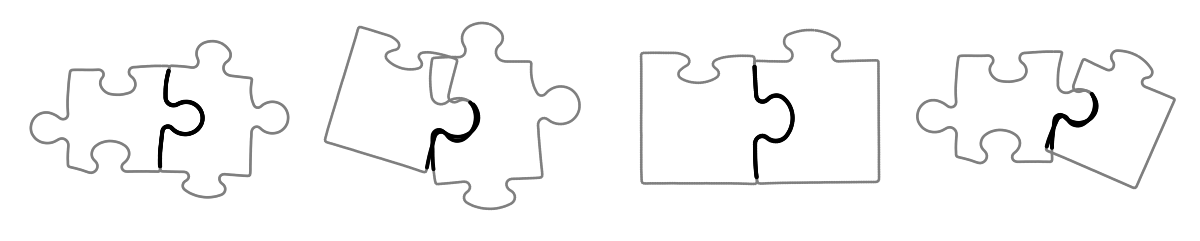
Thus, transformation consistency does not provide a complete filter to identify cycles in the assembly graph consisting of correct $\epsilon$ -fits. In order to eliminate incorrect transformation consistent cycles like the one in Figure 13, we introduce overlap consistency, a more stringent check on cycles in the comparison graph. Overlap consistency is motivated by the simple observation that a correctly assembled cycle will not have overlapping pieces.

Denote by $\text{int}(P_{i})$ the interior of the puzzle piece $P_{i}$ and let $P_{i_{1}},\ldots,P_{i_{k}}$ be a collection of pieces as before. In a perfect puzzle assembly the interiors of these pieces should not overlap as they are assembled. That is, all pairwise intersections of the open regions

\Omega_{j}=\text{int}(g_{i_{1}i_{2}}g_{i_{2}i_{3}}\cdots g_{i_{j-1}i_{j}}P_{i_{j}}),\quad j=1,\ldots,k,

should be empty. Since our assemblies will not be perfect, we impose a threshold test on the areas of these intersections. In order to account for puzzle pieces of varying size, our threshold is determined as a portion of the combined areas of the pieces being compared.

Definition 21.

Let $\Omega_{1},\ldots,\Omega_{k}$ be as above and let $\alpha^{*}>0$ and $\alpha^{*}_{ij}=\alpha^{*}\big(\text{area}(\Omega_{i})+\text{area}(\Omega_{j})\big)$ . If $\text{area}\big(\Omega_{i}\cap\Omega_{j}\big)<\alpha^{*}_{ij}$ for $i,j=1,2,\ldots,k$ , then the cycle $(P_{i_{1}},\ldots,P_{i_{k}},P_{i_{1}})$ will be called overlap consistent (with respect to $\alpha^{*}$ ). If all cycles in the cycle graph $P_{i_{1}},\ldots,P_{i_{k}}$ are overlap consistent, then the cycle graph $(P_{i_{1}},\ldots,P_{i_{k}})$ will be called overlap consistent.

Remark 22.

Checking overlap consistency is much more computationally intensive than transformation consistency, requiring at most $k(k-1)/2$ computations of the intersections of polygons for each cycle. To check overlap consistency for the whole cycle graph, these checks must be repeated for each of the $k$ starting points of cycles, naively resulting in a total of $k^{2}(k-1)/2$ overlap checks. In practice, most of these overlap consistency checks will fail before checking all $k(k-1)/2$ intersections. As needed, the computation time for overlap consistency checks can be reduced by first filtering cycles via a check on transformation consistency and by reducing the number of points in each puzzle piece by adjusting $\delta$ .

Example 23.

We return again to Example 17 and illustrate overlap consistency for cycles of length $4$ . As in Example 20 we use a modified comparison graph $G$ with $61$ edges and $1081$ cycles of length $4$ . With a threshold of $\alpha^{*}=\frac{1}{80}$ , exactly $6$ of these cycle graphs are overlap consistent, shown in Figure 14. These are the $6$ correct cycle graphs of length $4$ that we can expect to find in a perfect assembly.

To improve our optimal puzzle assembly, we incorporate cycle consistency information into the edge weights of the assembly graph. We do this by reducing the edge weights for those fits which appear in overlap consistent cycle graphs, increasing the likelihood that these fits are selected in the optimal puzzle assembly.

Definition 24.

Suppose that the $\epsilon$ -fit of $P_{i}$ and $P_{j}$ has weight $q_{ij}$ and appears in $c$ overlap consistent cycles. Choose $0<\beta^{*}<1$ , and assign a new weight $\overline{q_{ij}}=(\beta^{*})^{c}q_{ij}$ to the $\epsilon$ -fit. For rectangular puzzles, we will have $c=0,1,$ or $2$ . The graph $\overline{G}$ obtained from $G$ by assigning the new weights $\overline{q_{ij}}$ will be called the cycle consistent comparison graph.

Example 25.

We return to Example 17 for a final time and incorporate cycle consistency into the optimal puzzle assembly. Using the overlap consistent cycle graphs found in Example 23 and taking $\beta^{*}=\frac{1}{2}$ , we create the new overlap consistent comparison graph $\overline{G}$ . Taking a minimal spanning tree of this graph now results in a correct optimal puzzle assembly, shown in Figure 15. Hence cycle consistency is able to discern the correct $\epsilon$ -fits to include in the assembly where the quality measure alone is not.

5.3 The full puzzle assembly algorithm

We summarize our full method for automated puzzle assembly. Assembly results from applying this method to various example puzzles will be provided in Section 6.

Algorithm 26.

An algorithm for apictorial jigsaw puzzle assembly.

Input: A collection of (unprocessed) puzzle piece boundary curves.

Output: A collection of transformations intended to produce a correct puzzle assembly.

1.

Process the puzzle data. Choose an arclength separation $\delta$ and apply Algorithm 1 to the unprocessed pieces until arclength separation is uniform. In practice, this takes fewer than $10$ iterations. Let $P_{1},\ldots,P_{s}$ be the processed pieces.
2.

Compute integral invariants. Choose an integral invariant radius $r$ and apply Algorithm 6 to compute discrete integral area invariants $A_{1},\ldots,A_{s}$ for $P_{1},\ldots,P_{s}$ .
3.

Compute $\epsilon$ -fits for all piece pairs. Choose a fit threshold $\epsilon$ and apply Algorithm 9 to find the maximum length $\epsilon$ -fit $P_{i}\leftarrow P_{j}$ for each pair of pieces $P_{i},P_{j}$ . Store the quality data $\ell_{ij}$ , $d_{ij}$ , $\sigma_{i}$ , $\sigma_{j}$ and the Procrustres transformation $g_{ij}$ mapping $P_{j}$ to $P_{i}$ .
4.

Form the comparison graph. Choose a fit quality $q_{ij}=f(\ell_{ij},d_{ij},\sigma_{i},\sigma_{j})$ and form the weighted comparison graph $G$ as a complete graph edges $P_{i}$ and edge weights $q_{ij}$ . Optionally, the minimal spanning tree of $G$ can be computed and tested to see if it yields a correct optimal puzzle assembly.
5a.

Check cycle transformation consistency (optional, as a prefilter to overlap consistency). Choose thresholds $\theta^{*},\tau^{*}$ and a collection of cycles in $G$ to check for transformation consistency with respect to $\theta^{*},\tau^{*}$ .
5b.

Check cycle overlap consistency (optional, if comparison graph does not produce correct assembly). Choose a threshold $\alpha^{*}$ and a collection of cycles in $G$ (e.g. the transformation consistent cycles from 5) to check for overlap consistency with respect to $\alpha^{*}$ .
6.

Form the cycle consistent comparison graph. With $0<\beta^{*}<1$ , adjust the weights of $G$ to create the cycle consistent comparison graph $\overline{G}$ . The minimal spanning tree of $\overline{G}$ can then be tested to see if it yields a correct optimal puzzle assembly.

6 Results

Example 27.

Pictured in Figure 16 is the assembly of the 50 piece “Alphabet” puzzle, alphabet. Applying Algorithm 26 with $\delta=15,r=50,\epsilon=220,\sigma^{*}=115$ and quality

q_{ij}=d_{ij}/\ell_{ij}+\iota_{\sigma^{*}}(\min(\sigma_{i},\sigma_{j}))

yields this puzzle assembly. The optimal puzzle assembly obtained directly from $G$ is sufficient to solve this puzzle; no cycle consistency checks were performed. The entire computation (including segmentation of the puzzle images) required about 3 minutes on an Apple Macbook Air M1 8gb using Mathematica 12.3.1.0.

Example 28.

Pictured in Figure 17 is the assembly of the 46 piece “Rainforest” puzzle, rainforest. Applying Algorithm 26 with the same $\delta,r,\epsilon,\sigma^{*}$ and $q_{ij}$ as in Example 27 yields this puzzle assembly. The optimal puzzle assembly obtained directly from $G$ is sufficient to solve this puzzle; no cycle consistency checks were performed. The entire computation (including segmentation of the puzzle images) required about 3 minutes on an Apple Macbook Air M1 8gb using Mathematica 12.3.1.0.

Example 29.

Pictured in Figure 18 are two assemblies of the 100 piece “Safari” puzzle, safari. For both assemblies, we use $\delta=15,r=50,\epsilon=260,\sigma^{*}=205$ and the same quality $q_{ij}$ as in the previous examples. For the first assembly, no cycle consistency checks were performed, and the assembly is very incorrect. This assembly required 9 minutes Apple Macbook Air M1 8gb using Mathematica 12.3.1.0. For the second assembly, two stages of cycle consistency checks with cycle length 4 are performed: first transformation consistency with $\theta^{*}=\pi/30$ and $d^{*}=20$ , then overlap consistency with $\alpha^{*}=1/80$ on the transformation consistent cycles. In the comparison graph there are $9057744$ cycles of length 4, so this computation is intensive, requiring roughly 3 additional hours for cycle consistency checks. Note that the assembly is much improved, with only one piece misplaced.

Surprisingly, with the same values of $\delta,r,\epsilon$ and $\sigma^{*}$ , we can achieve a completely correct puzzle assembly by changing the quality to

q_{ij}=d_{ij}/\ell_{ij}^{3}+\iota_{\sigma^{*}}(\min(\sigma_{i},\sigma_{j})).

This change puts stronger weight on the length of the match, rather than just the average distance between paired points in the $\epsilon$ -fit. Shown in Figure 19 is the (correct) assembly for this quality, with no cycle consistency checks performed. This assembly required 9 minutes on the same hardware.

7 Conclusion

We have described a new method for automatic assembly of jigsaw puzzles. This method highlights the efficacy of integral area invariants for shape comparison, and uses combinatorial information about the collection of shape matches to better select which matches should be used for the puzzle assembly. As shown in Section 6, our method is effective at assembling traditional rectangular jigsaw puzzles, but does not rely on structural information about piece shape or arrangement. There are a number of interesting directions for further research.

In hoff2014automatic, related methods for puzzle assembly are shown to be effective on non-rectangular puzzles such as the Baffler Nonagon, baffler. This robustness to irregular assemblies is helpful for solving more general object reassembly problems. For reasons that are not yet clear, preliminary experiments applying our assembly method to non-rectangular puzzles have not yielded results as impressive as those of hoff2014automatic. It would be worthwhile to better understand this shortcoming, and to experiment with changes to Algorithm 26 to make it more effective on non-rectangular puzzles.

Our method of determining $\epsilon$ -fits involves exhaustive comparison of invariant signatures. This was a qualitative choice based on the goal of finding the longest match within a threshold of shape similarity. Other comparison methods or paradigms for comparison could be explored. Rather than enforcing a strict distance threshold, signature matches could be found using a more flexible notion of local sequence alignment, e.g. one that measures distance with allowance for errors or omissions, navarro2001guided. One could also search for alignments probabilistically, eddy2008probabilistic. Additionally, our shape comparisons were done independently; the fit of one pair of pieces does not affect the fit of another pair. This does not comport with reality, where a correct fit between a pair of pieces limits the further possible fits for those pieces. To reflect this fact in the algorithmic approach it may be possible to use multiple sequence alignment, feng1987progressive, which could seek non-overlapping alignments of a collection of signatures.

For large puzzles and large cycles, the cycle consistency process becomes computationally intensive since the number of cycles grows exponentially with both the number of vertices and the length of the cycle. Optimization of the approach to cycle consistency is needed to use it effectively to assemble puzzles larger than 100 pieces. One possible approach to this optimization would be to select cycles randomly to test, and update the cycle consistent comparison graph $\overline{G}$ dynamically. Random cycle selection could be done in an informed manner; prioritizing those consisting of $\epsilon$ -fits with better quality, for example.

There are a number of parameters that need to be determined for a successful puzzle assembly. Some of these parameters, such as the arclength resolution $\delta$ , the integral invariant radius $r$ and the comparison threshold $\epsilon$ , seem to depend primarily on the size of the puzzle pieces and not on the puzzle geometry per se. Others, such as the shape variation threshold $\sigma^{*}$ and the overlap threshold $\alpha^{*}$ depend on the geometry and arrangments of the pieces. It would be worthwhile to investigate how some of these parameters could be determined or optimized automatically. Along similar lines, one could investigate the relationship between parameter values and quality measurements of the fits. As can be seen in Example 29, the choice of quality can have a strong effect on the correctness of the assembly, and a more systematic method for choosing quality would be useful.

Finally, because the focus of this work was on the application of integral area invariants, the use of other invariant signatures (e.g. differential invariants, calabi1998differential; boutin2000numerically, or invariant histograms, brinkman2012invariant) in combination with our graph based assembly process was not systematically explored. It would be very interesting if other types of invariant signatures proved to be more (or less) effective in achieving correct puzzle assemblies.

8 Acknowledgements

The Carleton College Towsley Endowment provided funding that made this research possible. We would like to thank Peter Olver and Irina Kogan for helpful conversations. We are also grateful to Noah Goldman, Marshall Ma, and Jason Zhu for their contributions to an early version of this project.

9 Data Availability

Selected Mathematica code and puzzle image data is available at the second author’s website, http://people.carleton.edu/~rthompson. Additional code and data may be requested from the second author.

References

[1] Herbert Freeman and L Garder. Apictorial jigsaw puzzles: The computer solution of a problem in pattern recognition. IEEE Transactions on Electronic Computers, (2):118–127, 1964.
[2] Haim Wolfson, Edith Schonberg, Alan Kalvin, and Yehezkel Lamdan. Solving jigsaw puzzles by computer. Annals of Operations Research, 12(1):51–64, 1988.
[3] David A Kosiba, Pierre M Devaux, Sanjay Balasubramanian, Tarak L Gandhi, and K Kasturi. An automatic jigsaw puzzle solver. In Pattern Recognition, 1994. Vol. 1-Conference A: Computer Vision & Image Processing., Proceedings of the 12th IAPR International Conference on, volume 1, pages 616–618. IEEE, 1994.
[4] David Goldberg, Christopher Malon, and Marshall Bern. A global approach to automatic solution of jigsaw puzzles. In Proceedings of the eighteenth annual symposium on Computational geometry, pages 82–87. ACM, 2002.
[5] Daniel J Hoff and Peter J Olver. Automatic solution of jigsaw puzzles. Journal of mathematical imaging and vision, 49(1):234–250, 2014.
[6] Daniel J Hoff and Peter J Olver. Extensions of invariant signatures for object recognition. Journal of mathematical imaging and vision, 45(2):176–185, 2013.
[7] The rainforest giant floor puzzle, 48 pieces. Frank Schaffer Publications, 1992.
[8] The baffler nonagon, 69 pieces. Ceaco, Model 4211-2, 2010.
[9] Anna Grim, Timothy O’Connor, Peter J Olver, Chehrzad Shakiban, Ryan Slechta, and Robert Thompson. Automatic reassembly of three-dimensional jigsaw puzzles. International Journal of Image and Graphics, 16(02):1650009, 2016.
[10] Dinosaurs pouch puzzle, 12 pieces. Mudpuppy, Item 9780735331136, 2011.
[11] Michael Kass, Andrew Witkin, and Demetri Terzopoulos. Snakes: Active contour models. International journal of computer vision, 1(4):321–331, 1988.
[12] Marcella Manivel, Milena Silva, and Robert Thompson. Iterative respacing of polygonal curves. SN Computer Science, 3(5):1–9, 2022.
[13] Siddharth Manay, Byung-Woo Hong, Anthony J Yezzi, and Stefano Soatto. Integral invariant signatures. In European Conference on Computer Vision, pages 87–99. Springer, 2004.
[14] Siddharth Manay, Daniel Cremers, Byung-Woo Hong, Anthony J Yezzi, and Stefano Soatto. Integral invariants for shape matching. IEEE Transactions on pattern analysis and machine intelligence, 28(10):1602–1618, 2006.
[15] T Fidler, M Grasmair, H Pottmann, and O Scherzer. Inverse problems of integral invariants and shape signatures. Preprint, 2007.
[16] Thomas Fidler, Markus Grasmair, and Otmar Scherzer. Identifiability and reconstruction of shapes from integral invariants. Inverse Problems and Imaging, 2(3):341–354, 2008.
[17] Jeff Calder and Selim Esedoglu. On the circular area signature for graphs. SIAM Journal on Imaging Sciences, 5(4):1355–1379, 2012.
[18] Riley CW O’Neill, Pedro Angulo-Umana, Jeff Calder, Bo Hessburg, Peter J Olver, Chehrzad Shakiban, and Katrina Yezzi-Woodley. Computation of circular area and spherical volume invariants via boundary integrals. SIAM Journal on Imaging Sciences, 13(1):53–77, 2020.
[19] Temple F Smith, Michael S Waterman, et al. Identification of common molecular subsequences. Journal of molecular biology, 147(1):195–197, 1981.
[20] Peter H Schönemann. A generalized solution of the orthogonal procrustes problem. Psychometrika, 31(1):1–10, 1966.
[21] David W Eggert, Adele Lorusso, and Robert B Fisher. Estimating 3-d rigid body transformations: a comparison of four major algorithms. Machine vision and applications, 9(5):272–290, 1997.
[22] Alphabet giant floor puzzle, 50 pieces. The Learning Journey International, Item 436318, 2014.
[23] African plains safari jumbo jigsaw floor puzzle, 100 pieces. Melissa & Doug, Item 2873, 2006.
[24] Gonzalo Navarro. A guided tour to approximate string matching. ACM computing surveys (CSUR), 33(1):31–88, 2001.
[25] Sean R Eddy. A probabilistic model of local sequence alignment that simplifies statistical significance estimation. PLoS computational biology, 4(5):e1000069, 2008.
[26] Da-Fei Feng and Russell F Doolittle. Progressive sequence alignment as a prerequisite to correct phylogenetic trees. Journal of molecular evolution, 25(4):351–360, 1987.
[27] Eugenio Calabi, Peter J Olver, Chehrzad Shakiban, Allen Tannenbaum, and Steven Haker. Differential and numerically invariant signature curves applied to object recognition. International Journal of Computer Vision, 26(2):107–135, 1998.
[28] Mireille Boutin. Numerically invariant signature curves. International Journal of Computer Vision, 40(3):235–248, 2000.
[29] Daniel Brinkman and Peter J Olver. Invariant histograms. The American Mathematical Monthly, 119(1):4–24, 2012.