Reconstruction on Trees and Low-Degree Polynomials
Abstract
The study of Markov processes and broadcasting on trees has deep connections to a variety of areas including statistical physics, graphical models, phylogenetic reconstruction, Markov Chain Monte Carlo, and community detection in random graphs. Notably, the celebrated Belief Propagation (BP) algorithm achieves Bayes-optimal performance for the reconstruction problem of predicting the value of the Markov process at the root of the tree from its values at the leaves.
Recently, the analysis of low-degree polynomials has emerged as a valuable tool for predicting computational-to-statistical gaps. In this work, we investigate the performance of low-degree polynomials for the reconstruction problem on trees. Perhaps surprisingly, we show that there are simple tree models with leaves and bounded arity where (1) nontrivial reconstruction of the root value is possible with a simple polynomial time algorithm and with robustness to noise, but not with any polynomial of degree for a constant depending only on the arity, and (2) when the tree is unknown and given multiple samples with correlated root assignments, nontrivial reconstruction of the root value is possible with a simple Statistical Query algorithm but not with any polynomial of degree . These results clarify some of the limitations of low-degree polynomials vs. polynomial time algorithms for Bayesian estimation problems. They also complement recent work of Moitra, Mossel, and Sandon who studied the circuit complexity of Belief Propagation. As a consequence of our main result, we are able to prove a result of independent interest regarding the performance of RBF kernel ridge regression for learning to predict the root coloration: for some depending only on the arity, many samples are needed for the kernel regression to obtain nontrivial correlation with the true regression function (BP). We pose related open questions about low-degree polynomials and the Kesten-Stigum threshold.
1 Introduction
Understanding the computational complexity of random instances has been the goal of an extensive line of research spanning multiple decades and different research areas such as cryptography, high-dimensional statistics, complexity theory, and statistical physics. In particular, this includes work on satisfiability and refutation of random constraint satisfaction problems and on computational-to-statistical gaps. In much of this work, evidence for computational hardness is indirect because there are well-known barriers to proving hardness from classical worst-case assumptions such as NP-hardness [3, 7, 18, 2].
Recently, low-degree polynomials have emerged as a powerful tool for predicting computational-to-statistical gaps. Computational-to-statistical gaps are situations where it is impossible for polynomial time algorithms to estimate a desired quantity of interest from the data, even though computationally inefficient (“information-theoretic”) algorithms can succeed at the same task. Heuristics based on low-degree polynomials have especially been used in the context of Bayesian estimation and testing problems and partially motivated by connections with (lower bounds for) the powerful Sum-of-Squares proof system. More specifically, a recent line of work (e.g. [26, 25, 33, 5, 21, 36, 24, 9, 56]) showed that a suitable “low-degree heuristic” can be used to predict computational-statistical gaps for a variety of problems such as recovery in the multicommunity stochastic block model, sparse PCA, tensor PCA, the planted clique problem, certification in the zero-temperature Sherrington-Kirkpatrick model, the planted sparse vector problem, and for finding solutions in random -SAT problems. Furthermore, it was observed that the predictions from this method generally agree with those conjectured using other techniques (for example, statistical physics heuristics based on studying BP/AMP fixed points, see e.g. [13, 15, 39]). Some of the merits of the low-degree polynomial framework include that it is relatively easy to use (e.g. compared to proving SOS lower bounds), and that low degree polynomials capture the power of the “local algorithms” framework used in e.g. [22, 10] as well as algorithms which incorporate global information, such as spectral methods or a constant number of iterations of Approximate Message Passing [56].
In this work, we investigate the power of low-degree polynomials for the (average case) reconstruction problem on trees. We define the model and results in the next sections, but first give an informal summary. The goal for reconstruction on trees is to estimate the value of the Markov process at the root given its value at the leaves (in the limit where the depth of the tree goes to infinity), and two key parameters of the model are the arity of the tree and the magnitude of the second eigenvalue of the broadcast chain. Importantly, when it is known [31] that nontrivial reconstruction of the root is possible just from knowing the counts of the leaves of different types, whereas when such count statistics have no mutual information with the root (but more complex statistics of the leaves may) [46]. This threshold is known as the Kesten-Stigum threshold [31] and it plays a fundamental role in other problems, such as algorithmic recovery in the stochastic block model [1] and phylogenetic reconstruction [12]. Count statistics can be viewed as degree 1 polynomials of the leaves, which begs the question of what information more general polynomials can extract from the leaves.
In this paper, we answer this question in the limit case . Perhaps surprisingly, we find that the Kesten-Stigum threshold remains tight in the sense that even polynomials of degree for a small are not able to correlate with the root label (Theorem 6), whereas computationally efficient reconstruction is generally possible as long as is a sufficiently large constant (Theorem 5) and even when a constant fraction of leaves are replaced by noise. Building on the polynomial lower bound, we prove superpolynomiallly (in fact, subexponentially) many samples are needed for Gaussian Kernel Ridge Regression (KRR) to (weakly) learn to regression function which predicts the root from the leaf colorations (Theorem 21). This gives a simple and natural model where KRR provably fails that is outside the reach of existing lower bounds such as [29].
We also consider an analogous question where the tree is unknown, and the algorithm has access to i.i.d. samples of the Markov process where the root is biased towards an unknown label . In this setting, polynomials of degree again fail to correlate with the label , but we show that a simple algorithm, straightforwardly implementable in the Statistical Query (SQ) model [30], can recover in polynomial time (Theorem 11). Together, these results show that low-degree polynomials behave very differently in our setting than one might intuit based on previous work in related settings, such as in random constraint satisfaction problems or the block model.
1.1 Preliminaries
Notation.
We use the standard notation to denote an upper bound with an implied constant which is allowed to depend on ; the notation is similar for denoting a bound which is polynomial in its parameters. We let denote the total variation distance between distributions and normalized to be in and we use for the conditional mutual information of random variables conditional on ; see [11]. Given a vector and a subset of coordinates , we let denote the -dimensional vector corresponding to elements of .
Markov processes on trees.
We consider Markov processes with state space where is the size of the alphabet. Let be the transition matrix of a time-homogeneous Markov chain on , also referred to as the broadcast channel. For simplicity, we always assume henceforth that is ergodic (irreducible and aperiodic, see [17]) so it has a unique stationary distribution . Let be a rooted tree with vertex set , root , and where is the set of directed edges where is the parent of in the corresponding tree. The broadcast process on tree of depth with transition matrix and root prior a probability measure on is given by
When not otherwise indicated, is the stationary distribution for . The probability measure is a Markov Random Field on the tree . This means that if are subsets of the vertices of and all paths in from to pass through a third set of vertices , then and are conditionally independent given . This is called the Markov property, see e.g. [34]. In this paper, we focus on the setting of complete -ary trees (i.e. trees where every non-leaf node has children, and all leaf nodes are at the same depth). For the -ary tree of depth , we let be the set of leaves of the tree, i.e. the set of vertices in the tree at depth .
Definition 1.
We say that reconstruction is possible on the -ary tree with channel if
where the notation denotes the conditional law of under given event occurs, is the corresponding broadcast process on the depth tree with root and is the set of leaves.
When reconstruction is possible, the Bayes-optimal estimate of the root given the leaves can be computed in linear time by passing messages up the tree using the Belief Propagation algorithm [38]; for our purposes, we will not need the explicit formula for BP, which can be derived by applying Bayes rule, but refer the interested reader to the reference.
Given a matrix , we let denote the second-largest eigenvalue of in absolute value. The Kesten-Stigum (KS) threshold on the -ary tree is given by the equation . Building upon the original work of [31], it was shown that the KS threshold is sharp for the problem of count reconstruction on trees [46]: count reconstruction is possible when and impossible when .
Definition 2.
Let be the function which computes count statistics of an input vector with entries in . We say that count-reconstruction is possible on the -ary tree with channel if where the notation denotes the conditional law of given event , is the corresponding broadcast process on the depth tree and is the set of leaves on this tree.
Next, we define a notion of noisy reconstruction which plays an important role in this paper:
Definition 3.
For , we say that -noisy reconstruction is possible on the -ary tree with channel if where is the -noisy version of the broadcast process values , generated by independently for each vertex , setting with probability and otherwise sampling from 11 1 More generally, our results hold where the noise is from any full support distribution on ..
Note that in this definition, the law of can equivalently be written as where is the usual noise operator that independently resamples each coordinate of its input vector with probability , see e.g. [25, 50]. Finally, we recall from [28] the following standard definition: we say that robust reconstruction on the -ary tree with channel is possible if -noisy reconstruction is possible for every .
Low-degree polynomials and computational-statistical gaps.
As discussed in the introduction, low degree polynomials have been studied in a wide variety of contexts and settings. The recent work [51] showed that a version of the low-degree polynomial heuristic can predict the recovery threshold for natural Bayesian estimation problems, even when the recovery threshold is below the detection/testing threshold. In the present work, we will use the following key definition from their paper22 2 In our notation and are swapped compared to theirs, to match the convention in the broadcast process.
Definition 4 (Degree- Maximum Correlation [51]).
Suppose that where is a random vector in and is a random variable valued in . The degree- maximum correlation is defined to be
where is the space of degree at most multivariate polynomials in variables with real-valued coefficients.
As explained there, when the target label is a vector this definition can be applied with equal to each of the coordinates of . We note that we could rephrase our results in terms of a testing problem (as in much of the prior work on the low-degree method), but the above definition is more natural in our context (it avoids the need to introduce a “null distribution” ). In what follows, we omit the distribution the expectation is taken over as long as it is clear from context.
Instead of referring to polynomial degree directly, we usually use the following more convenient and equivalent definition. Suppose is a function . We define the (Efron-Stein) degree of to be the minimal such that there exist functions so that . One such minimal choice of is the Efron-Stein decomposition over , see e.g. [50]; this notion is also equivalent to the minimal degree polynomial representing where the variables are the one-hot encoding .
Reconstruction below the KS threshold.
In this paper, we will largely consider the problem of tree reconstruction with matrices with ; these exactly correspond to Markov chains which mix perfectly within a bounded number of steps. (There are many examples of such chains, for concreteness we give a very small example below in Example 14). Obviously, for such a chain , for any value of so such a model is always below the Kesten-Stigum threshold. Nevertheless, based on general results from existing work we know that near-perfect reconstruction of the root is possible (e.g. using Belief Propagation, which computes the exact posterior distribution [38]). This is true as long as is sufficiently large, and even with a constant amount of noise :
Theorem 5 ([46], Theorem 23 below).
Suppose is a the transition matrix of a Markov chain with pairwise distinct rows33 3 This condition is needed to rule out the case of e.g. a rank one matrix where reconstruction is clearly impossible. See also [46] for a more complex and precise condition. i.e. for all the rows and are distinct vectors. Let be arbitrary. There exists and such that for all , -noisy reconstruction is possible on the -ary tree and furthermore there exists a polynomial-time computable function valued in such that
where is the -noisy version of (see Definition 3).
1.2 Our Results
We study the power of low-degree polynomials for the problem of reconstructing the root of a Markov process. We consider this question in the context of two very closely related versions of the model which have both been extensively studied in the literature.
Reconstruction with a known tree. In this setting, the algorithm is given access to the leaf values from a single realization of the Markov process, and the goal is to estimate the root (where we are going to be interested in estimators which are low-degree polynomials of the leaves). The tree structure is known and the estimator/polynomial is allowed to depend on this information directly.
Reconstruction with an unknown tree. In this setting, the data is still generated by a complete -ary tree but the tree (in other words, the true ordering of the leaves) is unknown to the algorithm. This version of the model has been extensively studied due to close connections to the problem of phylogenetic reconstruction in biology, see e.g. [12, 20, 53]. Because this task is more difficult information-theoretically44 4 Note that in the single-sample case (), the information available to the algorithm would only be count statistics, which we know are insufficient for reconstruction below the KS threshold [43]., the algorithm is given access to i.i.d. samples from the broadcast model; we give a more precise definition of the model below.
Results for reconstruction with a known tree.
We consider the problem of tree reconstruction with matrices with ; these exactly correspond to Markov chains which mix perfectly within a bounded number of steps. As discussed above in Preliminaries, while such models are always below the Kesten-Stigum threshold for any value of the the arity , under fairly weak conditions on the reconstruction problem is still solvable for sufficiently large (Theorem 5). This is true even with noise and with a very simple reconstruction algorithm. As our main result we show that despite the algorithmic tractability of this problem, only very high degree polynomials are able to get any correlation with the root, in the same sense as Definition 4.
Theorem 6 (Corollary 16 below).
Let be the transition matrix of a Markov chain on and suppose that is such that is a rank-one matrix. For any function of Efron-Stein degree at most of the leaves and any prior on the root,
Remark 7 (Tightness).
For fixed , this result is tight up to the base of the exponent. When satisfies the assumption of Theorem 5, there is a function on a constant-degree subtree to recover the root and (by Fourier expansion) this is a polynomial of degree .
To interpret this result, observe that , so taking a constant, the Theorem shows that polynomials of degree even for an explicit constant fail to get any correlation with the root label. In comparison, in the previously mentioned contexts in the low-degree polynomials literature, the threshold for polynomials of degree matches the conjectured threshold for polynomial time algorithms (see e.g. [26, 25, 33]) and polynomials of degree correspond to conjectural thresholds for subexponential time algorithms (see e.g. [5, 16]).
A consequence: subexponential sample complexity lower bound for the RBF kernel.
As a consequence of our main result, we can analyze the behavior of kernel regression methods in our model. Kernel ridge regression is one of the canonical methods for solving supervised learning problems, including classification problems (see e.g. [48]). In many high-dimensional settings, it is believed that the function learned using a standard kernel (e.g. Gaussian or polynomial) is essentially a low-degree polynomial. Standard results in learning theory ([52]) imply that kernel ridge regression with a Gaussian/RBF (Radial Basis Function) kernel in dimensions can learn a degree polynomial on the hypercube or sphere using roughly samples. Establishing lower bounds on KRR is generally much harder. In certain particularly tractable settings (e.g. data from the uniform distribution on the hypercube) it has been recently shown explicitly that kernel regression (only) learns a low-degree polynomial [23, 37].
It seems plausible to guess that kernel ridge regression with a standard kernel will require subexponentially many samples of (leaf label, root label) pairs in order to learn to predict the root. We are able to verify this prediction in the case of the popular RBF (Radial Basis Function) kernel. See Section 4.1.1 for formal notation and background on kernel ridge regression.
Theorem 8 (Theorem 21 below).
Let be the transition matrix of a Markov chain on and suppose that is such that is a rank-one matrix, and suppose that has at least two nonzero entries. Then the for any color and prior for the root coloration , the following is true. Given i.i.d. samples from the broadcast model on the -ary tree with leaves and broadcast channel , where is a one-hot encoded vector of leaf colorations and is the centered indicator of the leaf coloration, we have that for any bandwidth and ridge parameter , for the output of ridge regression in RKHS space with those parameters and feature map , that with probability at least
provided that where is independent of the depth of the tree.
This establishes a new and illustrative example where KRR performs poorly in high dimensions, even though the ground truth is a relatively “simple” and the labels are closely related to the structure of the input data. Note that the conclusion implies that , i..e. kernel ridge regression does not significantly outperform the constant zero estimator (“null risk”) unless it is given at least a subexponential number of samples. Also, as with Remark 7 this result is tight up to the power of the exponent , since a subexponential degree polynomial exists which predicts the root well and it can provably be learned with subexponential number of samples by KRR [52].
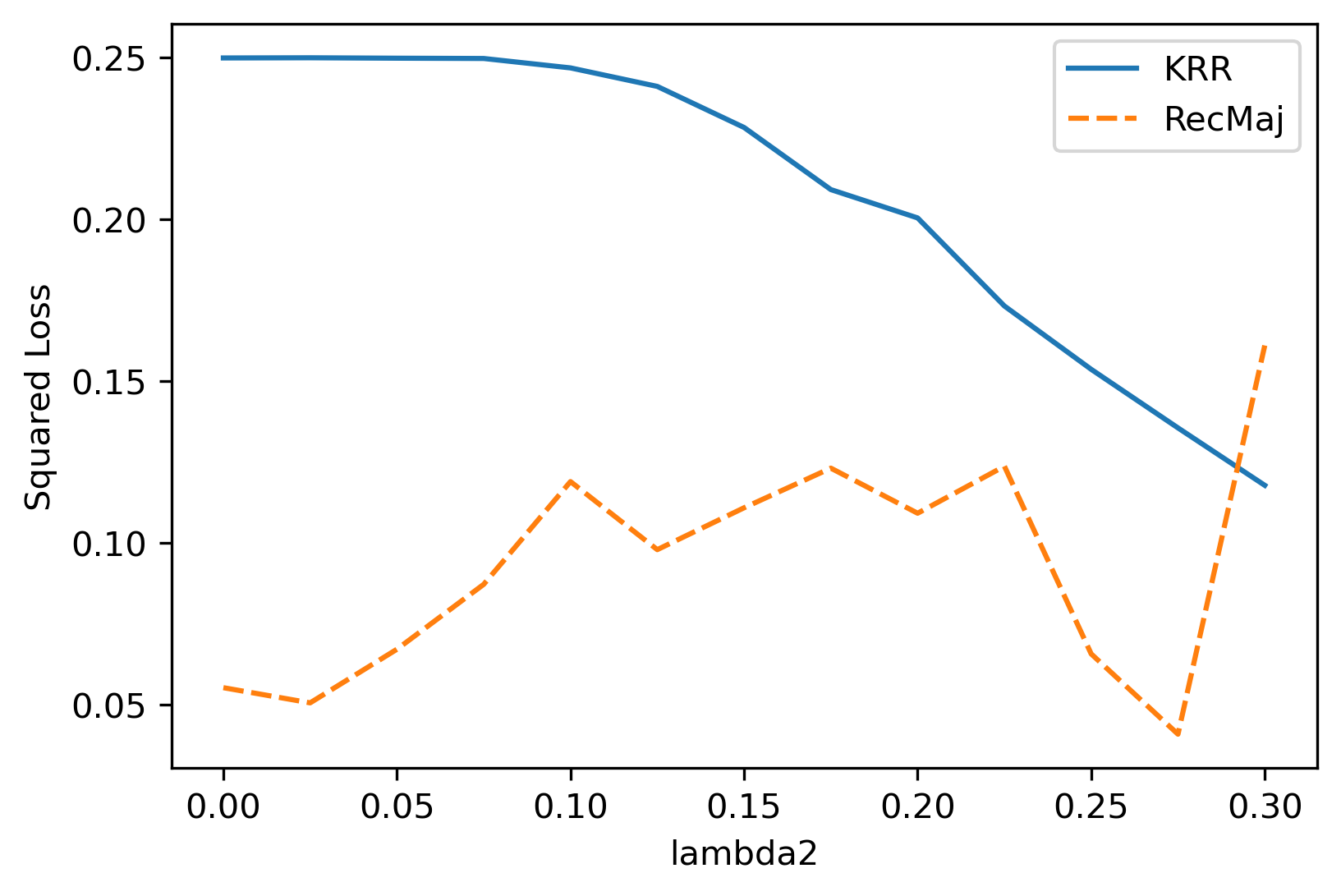
In Figure 1, we test kernel ridge regression in a simulation in both the case and : consistent with our result, KRR fails to beat the null risk when ; interestingly, it also fails for moderately small values of as well, which is related to the Open Problem we discuss later. In the figure, KRR is performed using 2000 i.i.d. samples of pairs with the one-hot encoded leaf colorations and the centered indicator that the root color is , as in Theorem 8. Bandwidth and ridge penalty are selected via grid search on a validation set. The results for the baseline (RecMaj) are averaged over 16000 samples.
Results for reconstruction with an unknown tree.
Formally, we consider the following variant of the generative model which is a variant of models in the phylogenetics literature. Briefly, in this model we generate i.i.d. realizations of the broadcasting model, where the tree is random and the prior on the root is biased towards a random root label. We include a parameter which can be used to add noise to the final output the of model, just as above.
Definition 9 (-Noisy Repeated Broadcast Model on Random Tree).
Let and let be a Markov chain on . Define by the following process:
- 1.
Sample , and is a random permutation. Let be the -ary tree on the set of leaves ordered by , so e.g. vertices and are siblings in .
- 2.
Sample i.i.d. from the -noisy broadcast process (see Definition 3) on with prior and transition matrix , where is a delta distribution on . Let .
The goal of the learning algorithm in the unknown tree model is this: given samples of the leaves of the broadcast process, encoded in , reconstruct the root label which the prior is biased towards55 5 We could also consider the model where the root label is always . The soft bias we consider is nicer for minor technical reasons, and seems natural given we allow to add noise elsewhere in the model.. We discuss the reasons for defining the model this way: 1. The permutation ensures that the coordinates of behave in a symmetric way, or equivalently that the order of those coordinates is not semantically meaningful; observe that if we omitted it, then the first coordinates would always be neighbors in the tree. This is standard in the phylogenetics literature [53] and this kind of symmetry is also assumed in the literature on low-degree polynomial hardness, see e.g. discussion in [24]; in sparse PCA this is analogous to how the support of the planted sparse vector is chosen uniformly at random among size- subsets. 2. The choice that root assignments are drawn from a tilted/biased distribution is different from the previous literature motivated by phylogenetics, where the root value is generally sampled fresh each time. This does not have a significant effect on how the algorithms used to estimate the tree work. The reason for our setup is to allow for straightforward comparison between SQ and low-degree polynomial models. If the root value was sampled from an unbiased measure each time, it would not make sense for an SQ algorithm to estimate it, since SQ has no concept of individual samples.
To be formal, we define the Statistical Query VSTAT oracle analogue of in the usual way [19]. The oracle is defined conditional on and the tree , so the order of leaves in the tree will be consistent between different calls to the oracle. As a reminder, vector-valued queries are implemented in the SQ model by querying each coordinate of the vector individually.
Definition 10 ( Oracle).
Let , , , and be as in Definition 9. Conditional on and the tree , we define to be an arbitrary oracle which given a query function , returns where where is arbitrary (can be adversarily chosen) such that .
We now state our results in this model. Just as in the known tree case, there is a relatively simple algorithm which achieves nearly optimal performance in this setting when and is a large constant, and furthermore this algorithm can straightforwardly be implemented in the SQ model described above. Establishing this requires proving a new result in tree reconstruction, since (for example) the setting which we care about rules out the use of Steel’s evolutionary distance (see e.g. [53, 40]) commonly used in reconstruction algorithms in phylogeny, as Steel’s distance is only well-defined for nonsingular phylogenies, and some kinds of tree models with singular matrices are actually computationally hard to learn [47].
Theorem 11 (Theorem 31 below).
Suppose is a the transition matrix of a Markov chain with pairwise distinct rows, i.e. for all the rows and are distinct vectors, and suppose . There exists and so that the following result holds true for the complete -ary tree with any depth . For any , there exist a polynomial time algorithm with sample complexity from the -noisy repeated broadcast model (Definition 9) which with probability at least : 1) outputs the true tree (equivalently, the true permutation ), 2) outputs such that . Also, this algorithm can be implemented using a oracle with and polynomially many queries.
Just as above, we show that the only polynomials which achieve any correlation at all with have to be at least degree :
1.3 Further Discussion
Related work: complexity of reconstruction on trees.
Our work follows a line of previous work which identified the Kesten-Stigum threshold as a potential complexity barrier in the context of the broadcast model on trees. The work [44] showed that algorithms that do not use correlation between different features (named “shallow algorithms”) cannot recover phylognies above the Kesten-Stigum threshold, where other (“deeper”) algorithms can do so efficiently; the motivation in [44] was to find simple data models where depth is needed for inference. More standard complexity measures were studied in [41] who obtained a number of results on the circuit complexity of inferring the root in the broadcast process. They conjectured that below the Kesten-Stigum threshold, inferring the root is -complete and proved it for one specific chain satisfying . Although there are some connections between low-degree polynomials and certain circuit classes [35], the results of this work and [41] are incomparable and the techniques for establishing the lower bound are very different. Finally, we note the work [27] which studied the power of message-passing algorithms on finite alphabets: they proved such algorithms fail to recover all the way down to the Kesten-Stigum threshold, even in the simplest case of the binary symmetric channel with .
Message passing vs. low-degree polynomials.
One of the attractive properties of the class of low-degree polynomials is that it generally captures the power of a constant (or sufficiently slowly growing) number of iterations of message-passing algorithms such as BP, AMP, and Survey Propagation (see e.g. [9] and Appendix A of [21]), which is interesting since a constant number of steps of these algorithms are indeed useful for many statistical tasks. On the other hand, in our models, belief propagation (which computes the exact posterior) succeeds with high probability whereas low-degree polynomials fail. This is not a contradiction: in our setting, BP requires iterations for the messages to pass from the leaves to the root and this is (as our main result shows) too large to simulate with low-degree polynomials.
SQ and Low-Degree Polynomials.
The recent work [8] established sufficient conditions for predictions to match between the Statistical Query (SQ) and low-degree polynomial heuristic, in a general setting. Nevertheless, in the unknown tree setting we consider above we saw that SQ algorithms perform significantly better than low-degree polynomials. The results of [8] cannot be immediately applied to our setting, because we have phrased the problem as an estimation problem instead of a testing (a.k.a. distinguishing) problem; however, this is itself not the reason for the discrepancy as we could rephrase our problem in terms of testing the color of the root. Instead, the reason seems to be due to the “niceness condition” needed for their theory to apply. They show that the niceness condition will be satisfied for noise-robust problems when the “null distribution” in the testing problem is a product measure. Our setup is indeed noise robust (see Theorem 5). However, if we rephrased our problem as a testing one the null distribution will be a graphical model (with no bias at the root) and not a product measure.
Recently there has also been interest in understanding lower bounds against kernel learning algorithms (including polynomial kernels), in part motivated by connections to neural networks, and this involves connections to the SQ framework. See e.g. [29] and references within. These methods can, for example, prove strong lower bounds against learning parities with kernel ridge regression since parities have large SQ-dimension. See also [32] for another example where polynomial degree lower bounds were established for a Bayesian inference task, though only polylogarithmic in the dimension.
Noise robustness and learning parities.
It was shown in [28] that the KS threshold is sharp for robust reconstruction, where we recall from above that (by definition) robust reconstruction on the -ary tree with channel is possible if for all noise levels , -noisy reconstruction is possible. At first glance, this appears similar to the idea in the low-degree polynomials literature that the model should be slightly noisy to rule out the example of learning parities (which can be solved in the noiseless setting by Gaussian elimination, but not when there is noise). In fact the two notions are quite different: the robust reconstruction result shows that reconstruction becomes impossible for large noise levels above a critical threshold , whereas for small (but fixed) the -noisy reconstruction problem often remains solvable — see Theorem 5. Our examples are fundamentally different to the parity example: (1) for the unknown tree version of our model, we showed that the problem is solvable with an SQ oracle whereas parities are well-known to be hard for SQ [6], (2) relatedly, the algorithms which solve our problems are not “algebraic” in nature, and (3) our results hold irrespective of adding a small amount of noise, whereas learning parities with any constant amount of noise is conjecturally hard [54]. Altogether, we can think of these results as suggesting a new, more nuanced picture of low degree vs. robustness to noise. Whereas before the main dichotomy in the computational complexity of inference literature has been between zero noise and any noise, in our model reconstruction algorithms such as BP can tolerate a small amount of noise, but fail when the noise level crosses some critical threshold. At least in our setting with , low-degree polynomials appear to capture the latter “large noise” behavior instead of the “small noise” difficulty of the problem.
Open Problem.
What happens when ? It is natural to wonder if the Kesten-Stigum threshold is sharp for low-degree polynomial reconstruction, analogous to how it is sharp for robust reconstruction. Our main lower bound result (Theorem 6) is consistent with this intuition. Also consistent with this intuition, our simulation result Figure 1 suggests that Kernel Ridge Regression may continue to fail for small but nonzero values of . Formally, we ask:
Question 13 (Kesten-Stigum is sharp for Low-Degree Polynomials?).
Suppose that and transition matrix are such that , i.e. we are below the Kesten-Stigum threshold. Let be an arbitrary function of such that as . Is it true that the degree- maximum correlation between the broadcast process at the leaves and the root in the sense of Definition 4 is asymptotically zero, i.e. ? Equivalently, is it true that
Here we make the common choice of looking at degree polynomials (see e.g. [26, 33]), but any degree is interesting.
With the same intuition, we ask if a similar result to Theorem 8, the lower bound for kernel ridge regression, holds below the Kestum-Stigum threshold — see Figure 1 for related simulation results, which support the failure of KRR for small values of . We note that in our experiment the threshold where KRR starts to work is much closer to . It is quite possible that this is a finite-depth effect since the experiment was done with a relatively shallow tree. Of course, if the sharp threshold is not the Kestum-Stigum threshold it would be extremely interesting to understand what the correct threshold is as a function of the broadcast model parameters.
2 Technical Overview
The detailed proofs of all results are given later. Here, we explain the high-level proof ideas, which we believe are relatively clean and conceptual. Before proceeding, we give the following concrete example of a Markov chain with and :
| (1) |
Since is rank one, it must be the case that .
Failure of low-degree polynomials (Theorem 6).
We want to show that any low-degree polynomial of the leaves of the broadcast tree fails to correlate with the root. In general, it may be very difficult to compute the maximal correlation among all low-degree polynomials; what makes it possible in our case is that the correlation is exactly zero. If is a color and is the prior at the root, we want to show . (Recall is the set of leaves and the leaf colorations.) The first step is to use linear of expectation to break into monomials: more formally, if is the Efron-Stein decomposition for a polynomial of degree , then to show the goal it clearly suffices to show
Crucially, the monomial is a function which depends only on a set of at most leaf colorations . Therefore, the result follows if we can show those leaves by themselves are independent of the root coloration. This is shown by performing an iterative trimming procedure on the minimal subtree spanned by the root and the leaves in : every time there is an isolated path of length (where is rank one: in the example above) all information is lost from the start of the path to its end. Using this idea and some elementary combinatorics, we can prove that if is small, the trimming procedure will delete everything, and so the root is indeed independent of these leaves.
Failure of RBF Kernel Ridge Regression (Theorem 8.)
This result builds on the low-degree polynomials result. First, we show that if the bandwidth parameter in the kernel is taken too small, then the output of Kernel Ridge Regression (KRR) is close to zero on a new test point and so it fails to learn anything. Otherwise, we can directly show that any function with a substantial high degree polynomial component has large RKHS norm. We can also construct an interpolator of the training data which has much smaller RKHS norm, by showing that every training sample has a small “fingerprint” which uniquely identifies it and is detectable with a low-degree polynomial. It then follows that whatever the output of KRR is, it must have a small RKHS norm and cannot correlate with the true regression function.
Success of noise robust reconstruction using “high degree” algorithms [46].
We briefly explain why noise robust reconstruction is possible with simple and computationally efficient algorithms. The key is to consider the case of a depth tree: because the rows of are distinct, if the degree of the tree is a sufficiently large constant, then by the Law of Large Numbers the empirical distribution of its children will be close to the row of corresponding to the state of the parent, letting us reconstruct the parent with say probability of success. Given this, it is not too hard to argue this argument works recursively and in the presence of a small adversarial noise. Note that this algorithm recursively integrates global information on the tree across multiple scales — in contrast, the lower bound used the fact that low-degree polynomials can only aggregate information between small sets of variables in a limited (linear) way.
Unknown tree results (Theorem 11 and Theorem 28).
The lower bound for low-degree polynomials in this setting can be reduced to the previous low-degree polynomial lower bound, which leaves proving that efficient (and SQ) algorithms can successfully solve this problem. Once we reconstruct the tree, we can run any algorithm for reconstructing the root given the leaves, e.g. the one described just above or BP. As far as reconstructing the tree, we first explain how to reconstruct the first layer. We prove that the joint distribution of any two leaves has enough information to tell us if they are immediate neighbors, which determines the location of all of their parents in the tree (such a test is easy to construct if we look at the generalized eigenvectors of ). Now that the bottom layer of the tree structure is determined, we use the fact that we have very good estimates of their parents colorations using the algorithm described before. Crucially, since that algorithm’s accuracy guarantee for reconstructing the internal node’s colors is very strong and does not decay as we go further and further up the tree, we can indeed apply this argument recursively to get the whole tree.
Implementing this algorithmic approach in the SQ framework is straightforward: at the end of the day it is based on computing the joint distributions of pairs of (estimated) vertex colorations, and those are all averages over the data. On the other hand, note that this method very strongly relies on the ability of an SQ algorithm to make adaptive queries, since the queries made are based on the partially reconstructed tree structure, which is unknown to the algorithm before it starts.
3 Organization
In the remaining sections we give full proofs of all results; there is no dependence on the Technical Overview as all the information there will be repeated here in more detail. In Section 4 we prove the results for known trees: in particular, this includes the main lower bound result, which is the failure of low degree polynomials for recovering the root; we also show how to deduce the RBF kernel lower bound using this. This is also where the RecMaj algorithm from Figure 1 is formally explained. In Section 5 we prove the results in the setting with an unknown tree; the main technical step is showing how to reconstruct the tree when using a sample-efficient algorithm, which can be straightforwardly implemented in SQ.
4 Known Tree: Upper and Lower Bounds
In this section, we prove a lower bound for arbitrary markov chains satisfying . From basic linear algebra (the existence of the Jordan Normal Form [4]), we know that if and only if is a rank one matrix for some , i.e. the Markov chain mixes perfectly in a finite number of steps. For concreteness, we give an example of such a chain with below.
Example 14 (Proof of Proposition 5, [42]).
The following Markov chain on states is a simple example of a chain with : we have
4.1 Failure of Low-Degree Polynomials
Theorem 15.
Let be the transition matrix of a Markov chain on and suppose that is such that is a rank-one matrix. Let be any subset of the leaves of the depth- complete -ary tree with root and let denote the broadcast process on with channel . Let be an arbitrary subset of the leaf nodes of this tree. If , then , i.e. is independent of the root value .
Proof.
Assume for contradiction that and . Let be the minimal spanning subtree of containing the root node and all of the elements of . (Equivalently, is the union of all of the root-to-leaf paths to .)
Recall that in our convention, the edges of the tree are directed from the parent to the child. We say that contains an isolated length directed path if there exists adjacent nodes contained in with for all , and such that nodes all have degree in .
We show that we can reduce to the case where contains no isolated length directed paths. Otherwise, let be as defined above and let be the subset of consisting of descendants of (note that by the definition of , is nonempty). Observe that
where the last equality follows by the Markov property (all nodes in are descendants of , so is independent of the root value conditionally on ).
Next, by the chain rule for mutual information
where the last equality follows from the fact that
where in turn the first equality follows from the Markov property ( is independent of conditional on and ) and the second equality follows because by the Markov property,
is a Markov chain where the rightmost channel has transition matrix , a rank-one matrix, so the conditional law of is the stationary measure of regardless of the value of , hence is conditionally independent of . Combining the above claims shows that
where ; by monotonicity of mutual information we in fact have
Repeating this argument recursively reduces to the case where has no isolated length paths.
Finally, if has no isolated length paths then every internal node of is either: (a) at depth at most , or (b) has an ancestor at graph distance at most away with degree at least . By induction, this implies that the number of nodes at depth in is at least twice as large as the number of nodes at depth . Since is the set of nodes in at depth , this implies that
which completes our proof by contradiction. ∎
Corollary 16.
In the setting of the previous Theorem, for any function of Efron-Stein degree at most of the leaves and any prior on the root,
Proof.
By linearity of expectation and the Efron-Stein decomposition,
where the last equality used the previous Theorem and the fact . ∎
4.1.1 A consequence: failure of RBF kernel regression with oracle tuning
Setting and notation.
We consider the performance of RBF kernel ridge regression (with arbitrary/oracle hyperparameter selection) for predicting the color of the root given the color of the leaves. As is customary, we encode the leaf vectors using a one-hot encoding, so the input to the regression is a list of i.i.d. samples where is the vector of one-hot encoded leaves, i.e. , and for an arbitrary fixed color , is the centered indicator that the root is colored .
Background on Kernel Ridge Regression.
We remind the reader of some standard facts about kernel ridge regression and the Gaussian/RBF kernel — see [52] for a reference. Given a kernel , training points , and responses , the kernel ridge regressor with ridge parameter is given by solving a linear equation
where is the kernel matrix, and the predicted response for a fresh data point is given by
As is well-known, kernel ridge regression with ridge parameter is equivalent to solving the ridge regression problem
| (2) |
with feature vectors lying in a certain Hilbert space. Note that with this parameterization the prediction for fresh data point would just be since is in the Hilbert space. In the case of the RBF kernel , the corresponding feature map for is
| (3) |
so that . Note that since .
Proof of the lower bound.
We now proceed to prove the subexponential RBF sample complexity lower bound in our setting. For an element of the RKHS, define the orthogonal projection operator onto the space of degree and higher polynomials by
From the definition, we first show that for large degree and bandwidth not too tiny, is very contractive when operating on feature embeddings .
Lemma 17.
For any and as defined in (3) with bandwidth parameter ,
Proof.
First observe that
by applying the multinomial theorem. Therefore,
and then the stated result follows from a nonasymptotic version of Stirling’s approximation. ∎
Next, we prove that there exists a relatively low-degree and low-RKHS norm polynomial which perfectly interpolates the training data, by showing that with high probability every sample has a small and unique “fingerprint” given by looking at a small set of well-separated leaves.
Lemma 18.
Let be the transition matrix of a markov chain on and suppose that is such that is a rank-one matrix, and suppose that has at least two nonzero entries. Then if is a set of leaves of distance at least from each other and are i.i.d. random vectors generated by the broadcast process with transition matrix , the probability that there exists such that is at most where is a constant depending only on .
Proof.
First, let be independent samples of the leaves from the generative model and let be such that the stationary distribution has at least two entries of size at least . For a set of leaves of distance at least from each other, we have by the Markov property that the entries of are independent from each other conditional on the values of the markov process for all vertices at height above the leaves; we see then that the conditional law of the leaves is which does not depend on , so in fact the leaves are unconditionally distributed according to the product measure . Then by independence,
where in the last step we used that regardless of the value of , has a probability at least of being different from it. ∎
Lemma 19.
For with , and and arbitrary, there exists of (Hilbert space) norm
such that
Proof.
Observe that
which for fixed , expands into a sum of at most many monomials of degree at most and with coefficient . Representing this expanded polynomial in the RKHS, using (3), then leads to the stated norm bound. ∎
We show that the overlap between two independent samples of the leaves from the model concentrates exponentially with a subgaussian tail:
Lemma 20.
Let be the transition matrix of a markov chain on and suppose that is such that is a rank-one matrix. Then if are two independent random vectors of leaf colorations generated by the broadcast process on the -ary tree with leaves and are the corresponding one-hot encodings, we have that
where is a constant not depending on .
Proof.
First, observe that if is smaller than , this bound can be proved trivially by shrinking , so henceforth we assume is larger than this. By the law of total probability, it is sufficient to prove the desired bound conditional on the colors where is the set of vertices at height above the leaves, and similar to the proof of Lemma 18 we observe by the Markov property that this makes the color of the set of children of any particular independent of the colors of all non-children of . This means that a sum of bounded independent random variables, and because we have that its expectation is , so the result follows immediately from Hoeffding’s inequality [55]. ∎
Theorem 21.
Let be the transition matrix of a markov chain on and suppose that is such that is a rank-one matrix, and suppose that has at least two nonzero entries. Suppose that . Then given i.i.d. samples from the broadcast model on the -ary tree with leaves and broadcast channel , we have that for any bandwidth and ridge parameter , for the output of ridge regression in RKHS space with those parameters, that with probability at least
provided that where is independent of (equivalently, independent of the depth of the tree).
Proof.
As usual, we will use that can be assumed larger than a fixed absolute constant without loss of generality. The proof is via case analysis on the bandwidth parameter .
First we make an argument which covers the case of small bandwidth parameter . Note that for any , almost surely since there are leaves and each leaf is one-hot encoded. By Lemma 20 and the union bound, with probability at least for any in we have
so
It follows that there exists such that if , then for and so by Gershgorin’s disk theorem and the fact that the diagonal of is all-ones, . Hence for the Kernel Ridge solution we have .
Consider a fresh test set of independently sampled pairs of leaf and root colorations where . Observe by Hoeffding’s inequality that with probability at least ,
where is a fresh one-hot encoded vector of leaf colorations sampled from the same distribution and where we used the fact that and to show that over the randomness of , almost surely, which we used in order to apply Hoeffding’s inequality. By repeating the argument used to show the off-diagonal entries of are small, we have with probability at least
hence by the triangle inequality we have with probability at least that
and recalling gives the result in this case.
Now we cover the remaining set of bandwidth parameters where . By the combination of Lemma 18 applied with and Lemma 19, we have that there exists such that for every
and
| (4) |
It follows that the output of KRR with any ridge parameter has norm at most the rhs of (4) (otherwise, replacing the output with would shrink the norm without decreasing the training error in (2)). Next, by Lemma 17 we have that for any and degree
so taking as in Corollary 16 where this equation defines and using that
we have that for any satisfying (4),
Since by Corollary 16 and Cauchy-Schwarz we have that
combining this with the bound on completes the proof. ∎
4.2 Success of noise-robust reconstruction using non-low-degree algorithms
Above we saw that when , very high degree polynomials are needed to get any estimate correlated with the root. Nevertheless, for “most” matrices with and for degree sufficiently large as a function there exists a simple recursive and noise-robust method which witnesses the fact that reconstructing the root is possible. If one likes, this recursive function can trivially be expressed as a polynomial: then it will be a very high-degree polynomial that is nonetheless robust to noise.
The reason for the qualifier “most” in the discussion above is that there are some degenerate for which the task is clearly impossible: e.g. if is rank one (so it does not depend on its input). There are other similar examples, e.g. the chain on 3 states which deterministically transitions from state to state , and such that at states and the chain flips a fair coin to transition to either state or . With this clarified, we can now state the known positive result for reconstruction.
Theorem 22 (Theorem 6.1 of [43]).
Suppose is a the transition matrix of a Markov chain with pairwise distinct rows, i.e. for all the rows and are distinct vectors. Then there exists such that for all , reconstruction is possible on the -ary tree.
A variant of the condition in this Theorem gives a tight characterization of Markov chains where reconstruction is possible on the infinite -ary tree for sufficiently large , see Theorem 2.1 of [46].
By revisiting the proof of Theorem, we get the following slightly more precise result which we will use in later sections. This result shows that for any desired accuracy , for sufficiently large degrees there exists a noise-tolerant estimator which reconstructs the root correctly with probability at least uniformly of the color of the root.
Theorem 23 (Proof of Theorem 2.1 of [46]).
Suppose is a the transition matrix of a Markov chain with pairwise distinct rows, i.e. for all the rows and are distinct vectors. Let be arbitrary. There exists such that for all , -noisy reconstruction is possible on the -ary tree and furthermore there exists a polynomial-time computable function valued in such that
where is the -noisy version of (see Definition 3).
Proof sketch.
As explained above, this result follows from examination of the proof of Theorem 2.1 in [46]. For the reader’s convenience, we summarize the main idea of the proof.
In the base case of a depth tree, reconstruction of the root with probability at least is possible provided is a suitably large constant, because by basic large deviations theory (Sanov’s Theorem [14]) the empirical distribution of the children will concentrate around the row of corresponding to the root label (which by assumption is distinct from all of the other rows). This procedure is also robust to a small amount of noise, which handles the case where and in fact even if the proportion of children assigned labels by the noise process choose their labels adversarially. When doing the induction, the result of the reconstruction process at lower levels of the tree can therefore (by conditional independence) be modeled as the true values with a small amount of adversarial noise and this allows the same argument to show that at each level each vertex is recovered correctly with probability at least (where we take ). ∎
Remark 24 (RecMaj in Figure 1).
The RecMaj algorithm in Figure 1 corresponds to the algorithm described in the above proof sketch: i.e. a recursive algorithm which to reconstruct the coloration of a vertex, looks at the reconstructions of its children, takes the empirical distribution, and picks the corresponding row of which is closest in norm.
4.3 Low-Degree Polynomials succeed above the KS threshold
The Kesten-Stigum threshold is the sharp threshold for count reconstruction defined earlier. The definition of count reconstruction informally says that there is a nontrivial amount of mutual information between count statistics at the leaves and the value of the Markov Random Field at the root. To relate count reconstruction to low-degree polynomials, we use the following more precise result:
Lemma 25 (Proof of Theorem 1.4 of [46]).
Suppose that . There exist coefficients for such that the random variable
satisfies
where is an unit-norm eigenvector of in its second-largest eigenspace, i.e. achieving , and such that
where are constants depending only on and (in particular, they are independent of the depth of the tree).
As a consequence of this, we immediately obtain that low-degree polynomials (in fact, degree 1 polynomials) have nontrivial correlation with the root above the KS threshold, in the same sense as Definition 4.
4.3.1 A Question: Bayes-Optimal Reconstruction
We saw above that degree-1 polynomials of the leaves are sufficient to achieve nontrivial correlation with the root, provided that the model we consider is above the KS threshold. A natural question is whether higher degree polynomials have a significant advantage over degree-1 polynomials for estimating the value of the root. Relevant to this question, we recall the following result and conjecture from [45] which concerns noise-robust recovery with the Binary Symmetric Channel (equivalently, the Ising model on trees without external field):
Theorem 26 (Theorem 3.2 of [45]).
There exists an absolute constant such that the following result is true. For let
and observe that . If , then for all and defined by the -noisy broadcast model,
in other words, if is fixed then in the limit of infinite depth the probability of reconstructing the root correctly is the same as in the noiseless case .
(Recall that the equivalence of the statement in terms of TV and in terms of maximum probability of reconstructing the root follows from the Neyman-Pearson Lemma [49].) This statement is conjectured to hold with [45] and as explained there, is closely related to Bayes-optimal recovery in the stochastic block model. Based on this, we ask the following question:
Question 27.
Do polynomials of degree achieve asymptotically Bayes-optimal recovery with the above channel when ? More precisely, does there exist a polynomial threshold function of degree which asymptotically achieves
where the rhs is the error of the Bayes-optimal estimator.
It seems likely the answer to this question is positive. The reason for this is the following: (1) if the conjectured strengthening of Theorem 26 is true, then it implies that the combination of a majority vote up to some depth and number of rounds of belief propagation achieves Bayes-optimal recovery, and (2) a constant or very slowly growing number of rounds of belief propagation can be simulated with low-degree polynomials (see Appendix of [21]), and the threshold used in the majority vote should also be approximable by polynomials. We state the conjecture with degree polynomials since this is informally considered to correspond to “polynomial time algorithms” in the low-degree framework [25, 33], but based on the above discussion it seems likely that a smaller degree than is sufficient, e.g. any degree going to infinity with may be sufficient.
5 Unknown Tree Setting
In this section, we show that for any channel satisfying the conditions of Theorem 23, i.e. such that for sufficiently large reconstructing the root is possible (in the known tree setting/in the usual sense), then in the unknown tree setting that a relatively simple algorithm succeeds at reconstructing the root with a polynomial number of samples, and this algorithm can be straightforwardly implemented in the SQ (Statistical Query) model with polynomial number of queries and error tolerance.
The key step in the algorithm for reconstructing the root is a method of reconstructing the tree, which lets us reduce to the known tree setting. This kind of problem has previously been extensively studied in the context of phylogenetic reconstruction with particular channels coming from biology, and for example algorithms with polynomial runtime and sample complexity are known in the case that is a nonsingular matrix [47]. In the present context, we are very interested in the case of singular matrices (e.g. those with ) so we cannot rely on existing results.
Model.
We remind the reader that in the unknown tree setting, we are in the model of Definition 9. This means that an unknown is sampled from , and the algorithm seeks to reconstruct given access to i.i.d. samples of the leaves generated by the broadcasting process with root prior , i.e. the root is biased/tilted towards the unknown . When we say the tree is “unknown” in this model, it means that the algorithm is not given a priori knowledge of the true order of the leaves, e.g. the algorithm does not know at the beginning whether coordinates and of correspond to siblings or to leaves far apart in the tree (this is completely analogous to the situation in phylogenetic reconstruction [53]). In the definition of this model, this is modeled by shuffling the order of the leaves by an unknown permutation ; note that this order is kept consistent between each sample.
5.1 Failure of low-degree polynomials
Theorem 28.
Let be the transition matrix of a Markov chain on and suppose that is such that is a rank-one matrix. If is arbitrary and is a polynomial with Efron-Stein degree strictly less than , then
where is as defined in Definition 9.
Proof.
Let for denote the prior on .
By linearity of expectation and the definition of Efron-Stein degree, it suffices to show the result for functions of the form where , where each is a function only of the coordinates of its input in . Since the samples are conditionally independent given the value of , we have
where in the first equality we used the law of total expectation, in the second equality we used the aforementioned conditional independence, in the third equality we crucially used that by Theorem 15 the low-degree polynomial is independent of the root value and thus , and in the last step we used that by definition. ∎
5.2 Reconstruction Algorithm
For , let or denote the th standard basis vector in . In both cases, the vector is a column vector.
Lemma 29.
Suppose that is a probability measure on and for all , then there exists a constant such that the following is true. Let for be defined by the broadcasting process on with prior at the root and channels corresponding to the transition matrix of an ergodic Markov chain. Then for all .
Proof.
Under the assumptions, there exists some such that for a probability measure. Because is the stationary distribution and the marginal law at any vertex is for some , it follows that . ∎
Lemma 30.
Suppose that are two descendants of node at graph distance from and random variables follow the Markov process on trees with transition matrix . Then
where is a diagonal matrix with entries the marginal law of , i.e. for .
Proof.
Using the law of total expectation and using by the Markov property that and are conditionally independent given , we have
where in the last equality we used the definition of and the definition of the broadcast process in terms of the transition matrix . ∎
Based on this, we can recursively reconstruct the tree when the degree is sufficiently large. We note that for other channels like the BSC channel, tree reconstruction methods often handle internal nodes by computing majorities of the nodes under them, which gives an unbiased estimate of the spin , but this technique is not applicable in our setting (it’s unclear that unbiased estimators exist). Nevertheless, we show that applying the estimator from Theorem 23 can be used in a similar way, provided the degree is sufficiently large.
Theorem 31.
Suppose is a the transition matrix of a Markov chain with pairwise distinct rows, i.e. for all the rows and are distinct vectors. If , additionally suppose that the prior on the root of the tree is the stationary distribution of . There exists and so that the following result holds true for the complete -ary tree with any depth . For any , there exist a polynomial time algorithm with sample complexity from the -noisy repeated broadcast model (Definition 9) which with probability at least :
- 1.
outputs the true tree (equivalently, the true permutation )
- 2.
outputs such that .
Also, this algorithm can be implemented in the Statistical Query (SQ) model using a oracle with and polynomial number of queries.
Proof.
Given that the algorithm can correctly output the true tree , the fact that it outputs the correct root label follows straightforwardly from Theorem 23 by using the algorithm specified in that result to estimate the root in each sample, and then taking the majority vote over those samples (which will succeed with high probability provided we take samples due to Hoeffding’s inequality), and this can approach can also clearly be implemented in the SQ model (the SQ query is the robust reconstruction function of the leaves which outputs a vector, so we take the expectation of this and look at the largest entry of this vector). In the remainder of the proof, we show how to correctly output the true tree with high probability.
We first prove the result in the case that and afterwards describe how to modify the argument straightforwardly when . Let be a right eigenvector such that . We start by describing the algorithm which computes the estimated tree from the bottom up: let be a parameter to be set later. Let denote the expectation over the empirical distribution of samples, so for any function we have .
- 1.
Base case: for all leaves define . Let and set to be neighbors in iff . This constructs the first layer of the tree .
- 2.
Recursive case: suppose that we have reconstructed the first layers of the tree (from the bottom), and the current layer of the tree has more than one element. For each pair of internal nodes at the current level of the tree, let be the set of leaves under these nodes and let where is as defined in Theorem 23. Let and set to be neighbors in iff . This constructs the next layer of the tree .
We now need to show that with total probability at least , . First we consider the behavior of the base case; for simplicity, we first describe the argument when . Observe that if and are siblings in at depth then by Lemma 30
where is a diagonal matrix encoding the marginal law of for any at depth , and similarly, if and are not siblings then they are at graph distance at least in so
which is smaller by a factor of . (Note, here we are using the fact that in the case , we additionally assumed the prior at the root is stationary and so the marginal law at every depth in the tree is the stationary distribution.) Observe that by Hoeffding’s inequality and the union bound we have that with probability at least that in the base case step, every entry of the matrix for every pair of leaves is within additive error of its expectation. It follows from this and Lemma 29 that if for a sufficiently large constant depending only on , is sufficiently small with respect to , and then in the base case the algorithm computes neighbors correctly. Observe that at each layer, if the algorithm has correctly reconstructed in all previous layers then the sets for all nodes in this layer are deterministic functions of , and hence so are the queries the algorithm makes to . By a similar application of the union bound and Hoeffding’s inequality as well as Theorem 23 and the assumption that is sufficiently large with respect to it follows that the algorithm succeeds at all subsequent layers as well.
Note that provided we take is sufficiently small, we can show the base case of the argument will still succeed by using the triangle inequality, and the inductive step in the argument will succeed because of Theorem 23.
Finally, in the case that , we let be a generalized eigenvector such that but . Note that such a vector must exist because, is an eigenvalue of algebraic multiplicity as is ergodic and , and because our assumption on rules out the case that is rank one, so it’s Jordan normal form must have at least one Jordan block with size at least and this corresponds to the existence of such a generalized eigenvector . Now observe for such a that if are siblings in at depth then
which by Lemma 29 is lower bounded by a constant , while if are not siblings,
Setting and defining the remaining constants similarly to above ensures the algorithm succeeds, by the same argument.
Note that in both the case and , the algorithm is implemented by taking the expectation of certain functions over the samples, so it is straightforwardly implementable with SQ queries by replacing the empirical expectation with the VSTAT oracle. ∎
References
- [1] Emmanuel Abbe. Community detection and stochastic block models: recent developments. The Journal of Machine Learning Research, 18(1):6446–6531, 2017.
- [2] Adi Akavia, Oded Goldreich, Shafi Goldwasser, and Dana Moshkovitz. On basing one-way functions on np-hardness. In Proceedings of the thirty-eighth annual ACM symposium on Theory of computing, pages 701–710, 2006.
- [3] Benny Applebaum, Boaz Barak, and David Xiao. On basing lower-bounds for learning on worst-case assumptions. In 2008 49th Annual IEEE Symposium on Foundations of Computer Science, pages 211–220. IEEE, 2008.
- [4] Michael Artin. Algebra. Pearson, 2011.
- [5] Afonso S Bandeira, Dmitriy Kunisky, and Alexander S Wein. Computational hardness of certifying bounds on constrained pca problems. In ITCS, 2020.
- [6] Avrim Blum, Adam Kalai, and Hal Wasserman. Noise-tolerant learning, the parity problem, and the statistical query model. Journal of the ACM (JACM), 50(4):506–519, 2003.
- [7] Andrej Bogdanov and Luca Trevisan. On worst-case to average-case reductions for np problems. SIAM Journal on Computing, 36(4):1119–1159, 2006.
- [8] Matthew Brennan, Guy Bresler, Samuel Hopkins, Jerry Li, and Tselil Schramm. Statistical query algorithms and low-degree tests are almost equivalent. In COLT, 2021.
- [9] Guy Bresler and Brice Huang. The algorithmic phase transition of random -sat for low degree polynomials. In FOCS, 2021.
- [10] Wei-Kuo Chen, David Gamarnik, Dmitry Panchenko, and Mustazee Rahman. Suboptimality of local algorithms for a class of max-cut problems. The Annals of Probability, 47(3):1587–1618, 2019.
- [11] Thomas M Cover. Elements of information theory. John Wiley & Sons, 1999.
- [12] Constantinos Daskalakis, Elchanan Mossel, and Sébastien Roch. Optimal phylogenetic reconstruction. In Proceedings of the thirty-eighth annual ACM symposium on Theory of computing, pages 159–168, 2006.
- [13] Aurelien Decelle, Florent Krzakala, Cristopher Moore, and Lenka Zdeborová. Asymptotic analysis of the stochastic block model for modular networks and its algorithmic applications. Physical Review E, 84(6):066106, 2011.
- [14] Amir Dembo and Ofer Zeitouni. Large Deviations Techniques and Applications. Springer, 2010.
- [15] Yash Deshpande and Andrea Montanari. Finding hidden cliques of size in nearly linear time. Foundations of Computational Mathematics, 15(4):1069–1128, 2015.
- [16] Yunzi Ding, Dmitriy Kunisky, Alexander S Wein, and Afonso S Bandeira. Subexponential-time algorithms for sparse pca. arXiv preprint arXiv:1907.11635, 2019.
- [17] Rick Durrett. Probability: theory and examples, volume 49. Cambridge university press, 2019.
- [18] Joan Feigenbaum and Lance Fortnow. Random-self-reducibility of complete sets. SIAM Journal on Computing, 22(5):994–1005, 1993.
- [19] Vitaly Feldman, Elena Grigorescu, Lev Reyzin, Santosh S Vempala, and Ying Xiao. Statistical algorithms and a lower bound for detecting planted cliques. Journal of the ACM (JACM), 64(2):1–37, 2017.
- [20] J. Felsenstein. Inferring Phylogenies. Sinauer, New York, New York, 2004.
- [21] David Gamarnik, Aukosh Jagannath, and Alexander S Wein. Low-degree hardness of random optimization problems. In 2020 IEEE 61st Annual Symposium on Foundations of Computer Science (FOCS), pages 131–140. IEEE, 2020.
- [22] David Gamarnik and Madhu Sudan. Limits of local algorithms over sparse random graphs. In Proceedings of the 5th conference on Innovations in theoretical computer science, pages 369–376, 2014.
- [23] Behrooz Ghorbani, Song Mei, Theodor Misiakiewicz, and Andrea Montanari. Linearized two-layers neural networks in high dimension. The Annals of Statistics, 49(2):1029–1054, 2021.
- [24] Justin Holmgren and Alexander S Wein. Counterexamples to the low-degree conjecture. In ITCS, 2020.
- [25] Samuel Hopkins. Statistical inference and the sum of squares method. PhD thesis, Cornell University, 2018.
- [26] Samuel Hopkins and David Steurer. Efficient bayesian estimation from few samples: community detection and related problems. In 2017 IEEE 58th Annual Symposium on Foundations of Computer Science (FOCS), pages 379–390. IEEE, 2017.
- [27] Vishesh Jain, Frederic Koehler, Jingbo Liu, and Elchanan Mossel. Accuracy-memory tradeoffs and phase transitions in belief propagation. In Conference on Learning Theory, pages 1756–1771. PMLR, 2019.
- [28] Svante Janson and Elchanan Mossel. Robust reconstruction on trees is determined by the second eigenvalue. The Annals of Probability, 32(3B):2630–2649, 2004.
- [29] Pritish Kamath, Omar Montasser, and Nathan Srebro. Approximate is good enough: Probabilistic variants of dimensional and margin complexity. In Conference on Learning Theory, pages 2236–2262. PMLR, 2020.
- [30] Michael Kearns. Efficient noise-tolerant learning from statistical queries. Journal of the ACM (JACM), 45(6):983–1006, 1998.
- [31] Harry Kesten and Bernt P Stigum. Additional limit theorems for indecomposable multidimensional galton-watson processes. The Annals of Mathematical Statistics, 37(6):1463–1481, 1966.
- [32] Frederic Koehler and Andrej Risteski. Representational power of relu networks and polynomial kernels: beyond worst-case analysis. arXiv preprint arXiv:1805.11405, 2018.
- [33] Dmitriy Kunisky, Alexander S Wein, and Afonso S Bandeira. Notes on computational hardness of hypothesis testing: Predictions using the low-degree likelihood ratio. arXiv preprint arXiv:1907.11636, 2019.
- [34] Steffen L Lauritzen. Graphical models, volume 17. Clarendon Press, 1996.
- [35] Nathan Linial, Yishay Mansour, and Noam Nisan. Constant depth circuits, fourier transform, and learnability. Journal of the ACM (JACM), 40(3):607–620, 1993.
- [36] Cheng Mao and Alexander S Wein. Optimal spectral recovery of a planted vector in a subspace. arXiv preprint arXiv:2105.15081, 2021.
- [37] Song Mei, Theodor Misiakiewicz, and Andrea Montanari. Generalization error of random features and kernel methods: hypercontractivity and kernel matrix concentration. arXiv preprint arXiv:2101.10588, 2021.
- [38] Marc Mezard and Andrea Montanari. Information, physics, and computation. Oxford University Press, 2009.
- [39] Sidhanth Mohanty, Siqi Liu, and Prasad Raghavendra. On statistical inference when fixed points of belief propagation are unstable. In IEEE 62st Annual Symposium on Foundations of Computer Science (FOCS), 2021.
- [40] Ankur Moitra. Algorithmic aspects of machine learning. Cambridge University Press, 2018.
- [41] Ankur Moitra, Elchanan Mossel, and Colin Sandon. Parallels between phase transitions and circuit complexity? In Conference on Learning Theory, pages 2910–2946. PMLR, 2020.
- [42] Elchanan Mossel. Reconstruction on trees: beating the second eigenvalue. Annals of Applied Probability, pages 285–300, 2001.
- [43] Elchanan Mossel. Survey: Information flow on trees. arXiv preprint math/0406446, 2004.
- [44] Elchanan Mossel. Deep learning and hierarchal generative models. arXiv preprint arXiv:1612.09057, 2016.
- [45] Elchanan Mossel, Joe Neeman, and Allan Sly. Belief propagation, robust reconstruction and optimal recovery of block models. In Conference on Learning Theory, pages 356–370. PMLR, 2014.
- [46] Elchanan Mossel and Yuval Peres. Information flow on trees. The Annals of Applied Probability, 13(3):817–844, 2003.
- [47] Elchanan Mossel and Sébastien Roch. Learning nonsingular phylogenies and hidden markov models. In Proceedings of the thirty-seventh annual ACM symposium on Theory of computing, pages 366–375, 2005.
- [48] Vidya Muthukumar, Adhyyan Narang, Vignesh Subramanian, Mikhail Belkin, Daniel Hsu, and Anant Sahai. Classification vs regression in overparameterized regimes: Does the loss function matter? Journal of Machine Learning Research, 22(222):1–69, 2021.
- [49] Jerzy Neyman and Egon Sharpe Pearson. Ix. on the problem of the most efficient tests of statistical hypotheses. Philosophical Transactions of the Royal Society of London. Series A, Containing Papers of a Mathematical or Physical Character, 231(694-706):289–337, 1933.
- [50] Ryan O’Donnell. Analysis of boolean functions. Cambridge University Press, 2014.
- [51] Tselil Schramm and Alexander S Wein. Computational barriers to estimation from low-degree polynomials. arXiv preprint arXiv:2008.02269, 2020.
- [52] Shai Shalev-Shwartz and Shai Ben-David. Understanding machine learning: From theory to algorithms. Cambridge university press, 2014.
- [53] Mike Steel. Phylogeny: discrete and random processes in evolution. SIAM, 2016.
- [54] Gregory Valiant. Finding correlations in subquadratic time, with applications to learning parities and juntas. In 2012 IEEE 53rd Annual Symposium on Foundations of Computer Science, pages 11–20. IEEE, 2012.
- [55] Roman Vershynin. High-dimensional probability: An introduction with applications in data science, volume 47. Cambridge university press, 2018.
- [56] Alexander S Wein. Optimal low-degree hardness of maximum independent set. arXiv preprint arXiv:2010.06563, 2020.