Hairy black resonators and the AdS4 superradiant instability
Abstract
The superradiant instability of Kerr-AdS black holes is studied by numerically solving the full 3+1 dimensional Einstein equations. We find that the superradiant instability results in a two stage process with distinct initial and secondary instabilities. At the end of the secondary instability the geometry oscillates at several distinct fundamental frequencies — a multi-oscillating black hole. The multi-oscillating black hole is remarkably close to a black resonator, albeit with a bit of gravitational hair. During the hairy black resonator epoch, the evolution of the horizon area is consistent with the exponential approach to a constant. By employing different seed perturbations in the initial Kerr-AdS geometry, we also demonstrate that the black resonator’s hair is not unique. In the dual quantum field theory description, rotation invariance is spontaneously broken and the energy density is negative in some regions, signaling an exotic state of matter which does not relax to a stationary configuration.
I Introduction
Waves with suitably tuned frequency and azimuthal quantum number scattering off rotating objects can be amplified via superradiance zeldovich; Starobinsky:1973aij. Of particular interest are rotating black holes, which contain ergoregions from which it is possible to extract energy and angular momentum Penrose:1969pc; Penrose:1971uk. Half a century ago it was pointed out that if waves can be confined with something akin to a mirror, so outgoing waves are reflected back inwards, then repeated interactions with a black hole can lead to exponential growth of the wave amplitude, potentially converting a significant fraction of the black hole’s mass into radiation Press:1972zz. The dynamics of superradiant instabilities — also known as black hole bombs — and their final state are of considerable of interest to a variety of fields including early universe cosmology Pani:2013hpa, particle physics and gravitational wave astrophysics Arvanitaki:2016qwi; East:2017ovw; East:2018glu; Siemonsen:2019ebd, astrophysical jets Brito:2015oca, and phase transitions in holographic duality Hartnoll:2011fn; Chesler:2014gya. For a detailed review of superradiance and black hole bombs see Ref. Brito:2015oca.
Perhaps the purest manifestation of a black hole bomb is that of the AdS4 superradiant instability. The dynamics of the system are governed by the 3+1 dimensional vacuum Einstein’s equations with a negative cosmological constant and asymptotically global AdS boundary conditions. The geometry contains a time-like boundary (conformally equivalent to sphere), which serves as a mirror from which gravitational waves are reflected inwards. Via holographic duality Maldacena:1997re, this system has a dual interpretation as a 2+1 dimensional strongly coupled quantum field theory living on the boundary.
For two decades it has been known that sufficiently rapidly spinning Kerr-AdS black holes are susceptible to superradiant instabilities Hawking:1999dp; Cardoso:2004hs. The spectrum of unstable modes in the Kerr-AdS spacetime was studied in Cardoso:2013pza. It was subsequently shown that any black hole in asymptotically AdS spacetime with an ergoregion — meaning a region where a Killing vector becomes spacelike — must be unstable Green:2015kur. It has been suggested that the AdS4 instability may have no end-state and can result in violations of cosmic censorship Niehoff:2015oga . Despite the long history of the AdS4 superradiant instability, the question of what the final state is has thus far remained elusive. Our goal in this paper is to study this long standing problem with numerical relativity simulations.
Suppose the dominant unstable mode in the Kerr-AdS spacetime has (complex) frequency and azimuthal quantum number . At a linear level the mode’s time and azimuthal angle dependence is then given by the exponential . Hence the associated gravitational wave rotates in at angular velocity while slowly growing in amplitude like . If the superradiant instability was a one stage process, with this mode and its harmonics merely plateauing after some time, the final state geometry would have a single Killing vector,
| (1) |
with . Black holes with single Killing vector — coined black resonators — were first constructed in Ref. Dias:2015rxy. Their geometry rigidly rotates with angular velocity , meaning they oscillate with a single fundamental frequency, and they are thermodynamically preferred over the Kerr-AdS solution with the same mass and angular momentum. However, they are also unstable Green:2015kur. Their angular velocities satisfy
| (2) |
which means is always spacelike near the AdS boundary, signaling the presence of an ergoregion. It is therefore reasonable to expect that additional instabilities occur at some stage of the evolution. A natural guess is that the superradiant instability results in the Kerr-AdS geometry transitioning to a black resonator, which then experiences its own distinct superradiant instabilities, thereby transitioning to another state.
Previously we numerically simulated the AdS4 superradiant instability and found evolution consistent with the transition of the Kerr-AdS geometry to an approximate black resonator geometry Chesler:2018txn. While secondary instabilities were also observed, numerical evolution was not carried out long enough to ascertain their end state, leaving the final fate of the system uncertain. Nevertheless, Ref. Chesler:2018txn found several unstable modes during the black resonator epoch. These modes oscillated at different fundamental frequencies and rotated with different angular velocities. This suggests that the final state has no continuous symmetries. In other words, it is reasonable to expect that the final state of the superradiant instability is a black hole geometry oscillating with several fundamental frequencies, and without a Killing vector or ergoregion. Following the nomenclature of Ref. Choptuik:2019zji, we will refer to black holes oscillating with multiple fundamental frequencies as multi-oscillating black holes. Multi-oscillating black hole solutions to an Einstein-scalar system in AdS5 were recently studied in Ref. Ishii:2021xmn.
One of the primary challenges in numerically simulating superradiant instabilities is the slow growth rates associated with unstable modes. Compounding this, the AdS4 superradiant instability has no symmetries to exploit, meaning one must numerically solve the full 3+1 dimensional Einstein equations. This is a common feature of superradiant instabilities with real fields, and consequently there are few simulations which reach the final state East:2018glu. In contrast, with complex fields it is possible to study superradiant instabilities in cylindrical symmetry East:2017ovw or charged superradiance with spherical symmetry Sanchis-Gual:2015lje; Bosch:2016vcp; Bosch:2019anc, thereby allowing much faster simulations.
To study the AdS4 superradiant instability one must employ fast and stable numerical algorithms. To this end, we use a characteristic evolution scheme we previously developed for asymptotically AdS spacetimes. This scheme — which has seen use in a wide variety of problems Chesler:2008hg; Chesler:2009cy; Chesler:2010bi; Heller:2012km; vanderSchee:2012qj; Adams:2013vsa; Heller:2013oxa; Casalderrey-Solana:2013aba; vanderSchee:2013pia; Casalderrey-Solana:2013sxa; Arnold:2014jva; Chesler:2015wra; Chesler:2015fpa; vanderSchee:2015rta; Chesler:2018txn; Ecker:2021ukv and is reviewed in detail in Ref. Chesler:2013lia — is remarkably efficient, allowing even five dimensional problems to be solved on a single CPU Chesler:2015wra. This efficiency is largely due to the fact that within the scheme, the apparent horizon can naturally be chosen to lie at some fixed radial coordinate. That is, the entire computation domain exterior to the apparent horizon and interior to the AdS boundary can be chosen to be a static spherical shell. This means the angular and radial directions can be discretized with tensor product grids, allowing efficient numerical integration and differentiation operations. Additionally, with tensor product grids it is easy to employ spectral and pseudo-spectral discretizations, which converge much faster than finite difference schemes boyd01. This allows far coarser grids to be used and ameliorates CFL instabilities, meaning one can also use a larger time step compared to a finite difference scheme. We also judiciously choose our initial conditions so that the instabilities are reasonably fast, but that the Kerr-AdS black hole is not too close to extremality. We do this because near-extremal black holes can develop structure near the horizon, requiring finer grids there and longer run times. For reference, each of our simulations runs in approximately five weeks on a 2020 MacBook Air.
We simulate the Kerr-AdS superradiant instability with two sets of seed perturbations, both with the same mass and spin. In both cases we find that the AdS4 superradiant instability results in a two stage process with distinct initial and secondary instabilities. At the end of the secondary instability the geometry is that of a multi-oscillating black hole with several distinct fundamental frequencies. The multi-oscillating black hole is remarkably close to a black resonator geometry, albeit with a bit of gravitational hair localized far from the horizon. We see no obvious signs of additional instabilities in the multi-oscillating epoch. Indeed, at late times the apparent horizon area is consistent with the exponential approach to a constant. Multi-oscillating black holes are therefore a plausible candidate for the endpoint of the superradiant instability. We also demonstrate that hairy black resonators are not unique and depend on initial conditions.
II Setup
We numerically solve the vacuum Einstein’s equations with negative cosmological constant . We set the AdS radius to unity. Our characteristic evolution scheme is reviewed in detail in Ref. Chesler:2013lia. Here we outline the details salient for characteristic evolution with spherical coordinates and an appropriate choice of basis functions.
Our metric ansatz takes the form,
| (3) |
with Greek indices running over the AdS boundary spacetime coordinates , where is time and and are the usual polar and azimuthal angles in spherical coordinates. The coordinate is the AdS radial coordinate, with the AdS boundary located at . Note lines of constant are infalling radial null geodesics affinely parameterized by . Correspondingly, the metric ansatz (3) is invariant under shifts in ,
| (4) |
for any function . We exploit this residual diffeomorphism invariance to fix the location of the apparent horizon to be at . This means horizon excision is performed by restricting the computational domain to .
Near the AdS boundary Einstein’s equations can be solved with the power series expansion,
| (5) |
The expansion coefficient is the AdS boundary metric (i.e. the metric the dual quantum field theory lives in). As a boundary condition we fix
| (6) |
where
| (7) |
is the metric on the unit sphere. This boundary condition means gravitational waves are reflected off the AdS boundary.
A convenient diffeomorphism invariant observable is the stress tensor in the dual quantum field theory, which is determined by via deHaro:2000vlm,
| (8) |
Note that Einstein’s equations imply is traceless, , and covariantly conserved,
| (9) |
where is the covariant derivative under the boundary metric .
Within our characteristic evolution scheme, evolution variables consist of the conserved densities , a gauge parameter used to shift the horizon to be at via Eq. (4), and the rescaled angular metric,
| (10) |
with lower case latin indices running over the angular directions . All other components of the metric are determined by non-dynamical equations, which are solved on each slice of constant . The rescaled metric satisfies
| (11) |
which means contains two independent degrees of freedom. These two degrees of freedom encode the two propagating degrees of freedom in gravitational waves. In our numerical simulations we decompose as follows,
| (12) |
where indices are raised with and is traceless, meaning . Note the expansion (5) and boundary condition (6) imply that near the boundary .
II.1 Discretization
We expand the angular dependence of all functions in a basis of scalar, vector and tensor harmonics. These are eigenfunctions of the covariant Laplacian on the unit sphere. The scalar eigenfunctions are just spherical harmonics .11 1 Note we employ the convention . There are two vector harmonics, , which read oldref
| (13a) | |||||
| (13b) | |||||
where has non-zero components and . is longitudinal, meaning it points in the direction of , and is transverse, meaning . There are three symmetric tensor harmonics . However, since is traceless, we only need the two traceless tensor harmonics, which read oldref
| (14a) | |||||
| (14b) | |||||
The scalar, vector and tensor harmonics are orthonormal and complete. Upon expanding SO(3) scalar, vector, and tensor components of the metric and boundary stress in terms of these basis functions, angular derivatives can be computed by differentiating the basis functions themselves. In order to efficiently transform between real space and mode space, we employ a Gauss-Legendre grid in with points and a Fourier grid in with points. For details see Ref. boyd01. The grid points are the zeros of the order Legendre polynomial,
| (15) |
and the associated integration weights read
| (16) |
Likewise, the grid points are
| (17) |
with associated integration weights . The transformation between real space and mode space can then be performed using Gaussian quadrature.22 2 Note that integration over can also be performed via Fast Fourier Transforms. However, with the small values of we employ in this paper, we have found Gaussian quadrature to be faster. Using Gaussian quadrature, the orthonormality of the scalar, vector and tensor harmonics is exact up to angular momentum . We choose .
We note that the mode expansions contain approximately half as many degrees of freedom as that which live on the real space grid. Because of this, we choose to use mode amplitudes as our evolution variables. When computing nonlinear products, we simply transform the mode amplitudes to real space first.
For the radial dependence of the metric, we employ an inverse radial coordinate and expand the dependence in a pseudo-spectral basis of Chebyshev polynomials. We employ domain decomposition in the direction with seven domains. The first domain interface lies at and the remaining interfaces are equally spaced between and . We use seven points in the domain closest to the boundary and 14 points in all other domains. Note that using fewer points in the domain closest to the boundary helps ameliorate CFL instabilities, thereby allowing larger time steps.
We evolve forward in time units using a order Runge–Kutta method with constant time step . To test convergence of our numerics we have also ran simulations with approximately 15% more grid points in each direction, and with 20% smaller time step. Likewise, we also increased the filter parameters and (discussed below) by approximately 15%. Reassuringly, these simulations, which were ran until time , which encompasses the times during which the most structure exists, produced results indistinguishable from those presented in this paper. In particular, the differences in Fig. 4 were far smaller than the widths of each line.
II.2 Filtering
An important practical matter is filtering short wavelength excitations artificially generated during numerical evolution. We apply a short wavelength filter directly to the time derivatives of the fields. Following Chesler:2013lia, to filter the radial direction, we simply interpolate the real space radial grid to a courser grid, and then reinterpolate back to the original grid. For the course grid we use the same domain interface locations, but just with fewer points. Specifically, we use one fewer point in the domain closest to the boundary, and two fewer points in all other domains.
To filter in the angular directions, at each time step we multiply the time derivatives of the mode amplitudes by the filter function
| (18) |
where
| (19) |
This function, plotted in Fig. 1, is ostensibly a regularized step function. Note that at we have and at we have . Hence this filter does not appreciably modify low angular momentum modes (e.g. those with ).
| IC | ||||
|---|---|---|---|---|
| A | ||||
| B |
We note that our decomposition of the angular metric (12) and use of only traceless tensor harmonics is different from our previous study of the AdS4 superradiant instability Chesler:2018txn. In particular, in Ref. Chesler:2018txn we expanded in a basis of three tensor harmonics, with the additional one being proportional to , and imposed the constraint (11) numerically during each time step. However, imposing the constraint (11) involves nonlinear operations which can themselves numerically excite high angular momentum modes. While this can be ameliorated by employing a stronger filter than that used in this paper, the cost of doing so is reducing the effective angular resolution for a given value of . Hence, while our value of is essentially the same as that used in Ref. Chesler:2018txn, our effective angular resolution is superior.

II.3 Initial data
The Kerr-AdS solution is parameterized by mass and spin parameters and , and the AdS radius , which we have set to unity. For initial data we choose
| (20a) | |||||
| (20b) | |||||
where the superscript “Kerr” refers to the metric and boundary stress of the Kerr-AdS solution. If , then the resulting geometry is exactly that of the Kerr-AdS solution. Hence, with these initial conditions the superradiant instability is seeded by non-vanishing . We choose
| (21a) | |||||
| (21b) | |||||
Therefore, our initial conditions are determined by the mass parameter , spin parameter , and the mode amplitudes . Note that our choice of yields vanishing contribution to the total mass and angular momentum of the system. Hence the mass and angular momentum are identical to that of the Kerr-AdS solution with mass parameter and spin parameter .
We employ mass and spin parameters
| (22) |
and two sets of mode amplitudes given in Table 1, which we will refer to as initial condition (I.C.) A and B. Note our chosen masses and spins differ from those used in our previous work Chesler:2018txn by .
III Results
We begin by showcasing results for I.C. A. In the top panel of Fig. 2 we plot snapshots of boundary energy density at eight times between and . Note that the color scaling is different at each time. By a small amplitude excitation is visible. At subsequent times more structure develops via the excitation of higher modes, with different modes rotating in at different angular velocities. Nevertheless, by most of this structure has relaxed and the energy density approximately rotates rigidly at constant angular velocity. As we elaborate on further below, there are also tiny excitations with rotating at different angular velocities. These tiny excitations are responsible for small differences seen in the energy density peaks at times and .
To quantify the growth of different modes, including their frequency content, we define the mode amplitudes
| (23) |
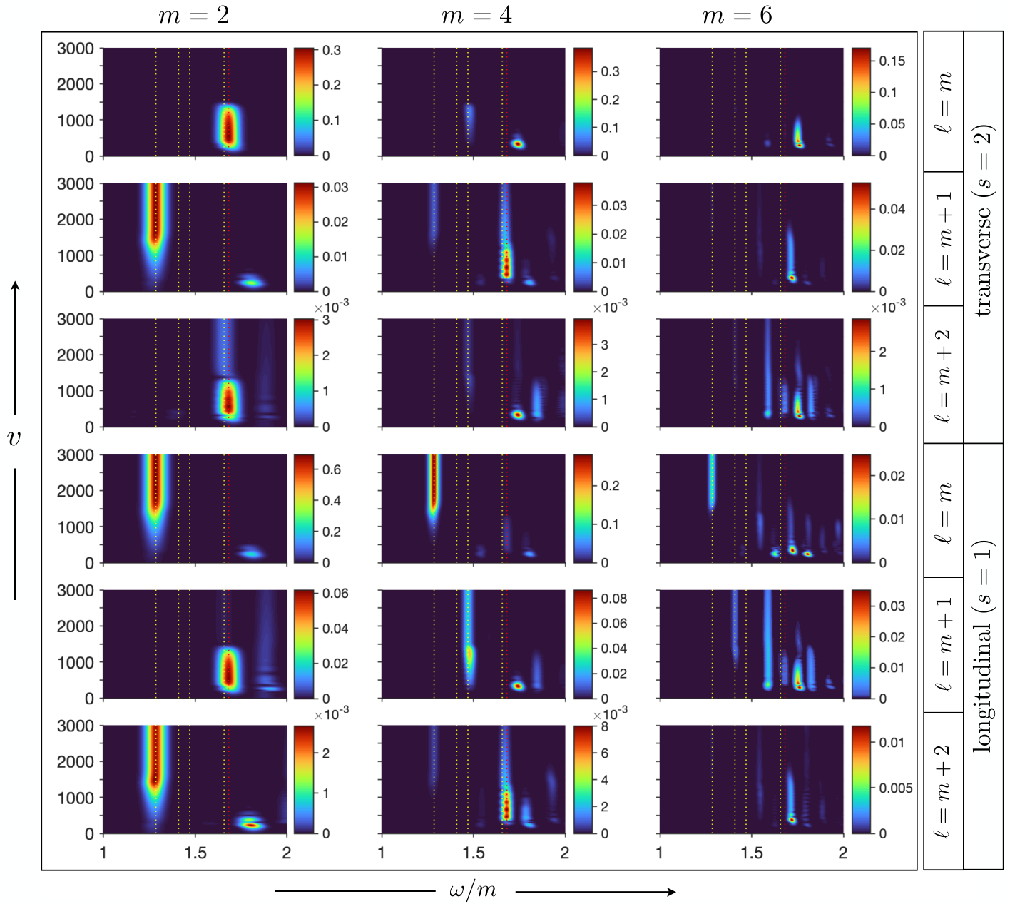
where is a Gaussian window function with width 15, and the vector spherical harmonics are given by Eq. (13). and are essentially the Fourier space amplitudes of the longitudinal and transverse components of the momentum density, respectively. More precisely, is the short-time Fourier transform of the vector spherical harmonic transform of the momentum density.
In all of our simulations we see no significant growth in with or odd . We therefore focus on even . Plotted in Fig. 3 are spectrograms showing as a function of and for and . All plots are on the same scale. Note is the angular velocity of a mode with frequency and azimuthal quantum number . At sufficiently late times the mode amplitudes decay everywhere except in the vicinity of a few fundamental frequencies. The four yellow dashed lines in Fig. 3 lie at frequencies , where is approximately constant at late times. These angular velocities are
| (24) |
Additionally, the red dashed line shows
| (25) |
The mode amplitudes evaluated along the dashed curves are shown below in Fig. 4. Note that the left and right columns in Fig. 4 show identical data, with the left column employing a logarithmic scale while the right column uses a linear scale.

From Figs. 3 and 4 it is evident there are two distinct epochs of growth in , which we shall refer to as initial and secondary instabilities Chesler:2018txn. The initial instability is due to superradiant instabilities in the Kerr-AdS geometry. Our numerics are consistent with an initial instability in the channel with complex frequency
| (26) |
The growth of begins to slow at , while also slightly shifting in frequency, and reaches its peak amplitude around . During the subsequent interval, , there is a plateau-like structure in . It is also during this time interval that the secondary instability kicks in, with
| (27) |
Note that the exponential growth of and is not as crisp as that of .
The fact that is the largest amplitude mode at the early stages of the secondary instability suggests that the intermediate state is an excited black resonator. However, it is noteworthy that near there are additional modes excited with amplitudes comparable to , but with fundamental frequencies different from . See Fig. 3. We comment on this further below in the Discussion section.
As seen in both Figs. 3 and 4, after , begins to precipitously decay while , , and approach constants shortly thereafter. Actually, all three of these modes are decaying extremely slowly at late times, with , although this is nearly impossible to see in Fig. 4. We are unsure if this tiny decay rate is real or a numerical artifact. We comment on this below in the Discussion section. At we have,
| (28a) | ||||||
| (28b) | ||||||
It is noteworthy that is nearly 30 times larger than the next largest mode, . If was the only angular velocity excited, then the geometry would be a black resonator. Evidently, the final state of our numerical evolution is a black resonator with a small amount of gravitational hair.
A natural question is where in the bulk is the black resonator’s hair localized? Is it localized near the boundary or is it spread throughout the bulk, including near the horizon? To answer this question we consider the Kretschmann scalar . Near the boundary , indicating that itself is not a good probe of near-boundary excitations. We wish to construct a quantity from which has a nontrivial limit near the boundary and which can discriminate contributions from different frequencies, including those with small mode amplitudes. To this end we take the short-time Fourier transform of the difference ,33 3 Due to memory constraints relevant for the calculation of , here we use a Gaussian window function with width 10.
| (29) |
and then average over the angular directions,
| (30) |
vanishes near the boundary and is insensitive to the precise value of (at sufficiently late times). The dimensionless ratio
| (31) |
has a nontrivial boundary limit and measures the amplitude of a bulk mode relative to the zero frequency limit.
In Fig. 5 we plot at time as a function of the radial coordinate and frequency . The four yellow lines superimposed on the figure correspond to the four angular velocities shown in Fig. 3 and listed in Eq. 24. The black lines show harmonics of the black resonator fundamental frequency, . Note that the color scaling is on a logarithmic scale. As is evident from the figure, is peaked at several discrete frequencies, with the largest peaks at and the black resonator’s fundamental frequency. The peaks corresponding to the black resonator’s hair are largest at large radii and smallest at the horizon (). In particular, at the horizon everywhere except near and the black resonator’s fundamental frequency and harmonics. In contrast, at , the peak at has amplitude . This signals that the black resonator’s hair is concentrated away from the horizon. Similar behavior was seen in Ref. Bosch:2016vcp, where the final state of the (spherically symmetric) charged AdS superradiant instability was studied.
Plotted in Fig. 6 is the apparent horizon area (left panel) and its time derivative (right panel), both normalized by the area of the associated Kerr-AdS black hole. To increase the fidelity of the plots of , as well as smooth out short time structure in due to individual superradiant amplification cycles, we compute by convolving with the time derivative of a normalized Gaussian with width 8. The two dashed lines in the right panel are simply the squares of the exponential curves seen in the and panels of Fig. 4. Evidently, during both the initial and secondary instabilities, the horizon area grows roughly as the square of the these modes. Note that decreases exponentially at late times. At the horizon area is 11% larger than that of the Kerr-AdS black hole with the same mass and spin.
Finally, we turn to evolution generated by our second initial condition. I.C. B has the same energy and angular momentum as I.C. A, but different initial seed perturbations. It turns out that many of the features of the resulting solutions are identical, both qualitatively and quantitatively. The resulting spectrogram for I.C. B looks strikingly similar to that shown in Fig. 3, with angular velocities identical to those found with I.C. A. Also included in Fig. 4 are the amplitudes obtained with I.C. B. During the initial and secondary instabilities the exponential growth rates are the same for both sets of initial conditions. Likewise, as shown in Fig. 6, and also have similar structure for both sets of initial conditions. Remarkably, the final values of , , and are also nearly identical for both set of initial conditions. Moreover, the final apparent horizon areas agree at order 1 part in .
Despite these similarities, the final state obtained with I.C. B is in fact distinct from that obtained with I.C. A. One difference lies in relative phase shifts between different modes. Define the phases
| (32) |
In order the exclude the possibility that the phases of our two solutions are merely related by a shift in and/or , we define the weighted phase differences
| (33) | |||||
| (34) | |||||
It is easy to check that and are invariant under shifts in and . If the late-time solutions generated by different initial conditions are identical, then they must have identical and at late times.
In Fig. 7 we plot and . The saw-tooth like structure seen in both plots is due to the fact that the phases are not continuous functions of time. For both sets of initial conditions and approach constants at late times. However, these constants are different for each initial condition. This demonstrates that the gravitational hair obtained with I.C. A is distinct from that generated with I.C. B. Simply put, the final state of our evolution is sensitive to seed perturbation in the Kerr-AdS geometry.
IV Discussion
It is remarkable that after starting in the Kerr-AdS geometry, and then having many large modes excited — as is evident from the plots of the energy density seen in Fig. 2 — that the geometry finds its way to a hairy black resonator state. Is a hairy black resonator, or more generally a multi-oscillating black hole, the final state of the superradiant instability? While our numerics are certainly consistent with this — mode amplitudes and the horizon area appear to plateau — we cannot exclude other possibilities. For example, it is always possible there are additional instabilities which are too small to be observed with our current numerical simulations. Likewise, its always possible there are instabilities in other channels not probed by our limited set of initial conditions.
Even if the final state is a hairy black resonator, it is possible the hair could undergo nontrivial slow dynamics. For example, the hair could decay or different modes could interact via nonlinear couplings, resulting in slow changes to the hairy mode amplitudes. We do see some evidence of slow mode amplitude dynamics in our simulations. The hairy modes seen in Fig. 4 all are decaying very slowly at late times, with . Additionally, we do see a tiny amount of late time growth in , which roughly grows like . This mode has angular velocity , which only differs from by . However, while these tiny rates could indicate interesting hairy dynamics (or even instabilities of the black resonator itself), they lie at the threshold of fidelity of our current numerical simulations. Indeed, we have also ran short duration simulations of our final state at 15% reduced resolution and found these rates to change significantly. To help assess whether the time dependence of these mode amplitudes is physical, it would be useful run simulations with different discretization and filtering schemes (e.g. cubing the sphere as opposed to using spherical harmonics), as well as long duration high resolution simulations.
We have also ran short duration simulations of a variety of perturbations of our final state. In doing so we found that after initial transients decay, the hairy mode amplitudes become approximately constant, just as seen in Fig. 4. However, we have found that the associated constants are sensitive to the perturbations and can differ by O(1) factors from those seen in Fig. 4. Notably however, these solutions have virtually identical horizon areas: all simulations resulted in the same horizon area at order 1 part in . This presumably reflects the fact that, as highlighted in Fig. 5, the hair is localized near the boundary, meaning it does not affect the near-horizon geometry.
It would clearly be of considerable value to study the mode spectrum of black resonators. First, it would be interesting to see how instabilities and decay rates of the black resonator associated with our final state compare with our numerical simulations. Second, it would be interesting to compare our intermediate state to a black resonator. While the spectrograms in Fig. 3 demonstrate that the intermediate state is initially dominated by a single angular velocity, , there are other modes appreciably excited with different angular velocities. This observation alone does not exclude the possibility that the intermediate state is an excited black resonator. Indeed, far-from-equilibrium black branes in AdS5 are well-approximated by large amplitude linear perturbations on top of a stationary background Heller:2012km. To solidify the intuition that the the intermediate state is an approximate black resonator, it would be useful to compare the black resonator spectrum to the spectrum of decaying and growing modes seen during the intermediate stage of our evolution. Finally, it would also be interesting to understand why instabilities associated with the intermediate state are strong, while none are visible in our final state. At the boundary our intermediate state is dominated by transverse modes whereas our final state is dominated by longitudinal modes. It is possible that instabilities associated with these two different types of black resonators could be qualitatively different.
We have only studied evolution with a single set of masses and spins. A natural question then is how generic are our results? Is the resulting multi-oscillating black hole always close to a black resonator? Its noteworthy that our previous work, Ref. Chesler:2018txn, which studied evolution with a different mass and spin, resulted in during the intermediate stage of the evolution. This suggests it is possible that the final state can be a multi-oscillating black hole which is significantly different from a black resonator. Simulating such a scenario likely requires higher resolution and longer runtimes than the simulations presented in this paper.
Finally, via AdS/CFT duality our results also have interesting consequences for quantum field theory. Firstly, the existence of the AdS superradiant instability implies that rotation invariance is spontaneously broken in the dual field theory. This behavior evidently only occurs in small systems, where there is are dual superradiant instabilities. From field theory arguments alone, we do not know why one should have expected this. Second, both sets initial conditions studied in this paper yield evolution with negative energy density. This was also found in Ref. Chesler:2018txn. This indicates that the dual quantum field theory state has exotic properties. Regions of negative energy density have also been seen in the holographic models studied in Athanasiou:2010pv; Casalderrey-Solana:2013aba; Chesler:2015fpa; Horowitz:2014hja. Finally, it is remarkable that the system does not appear to approach a stationary configuration despite having a large entropy. It would be interesting to explore to what extent, if any, hairy black resonators correspond to thermal states in the dual quantum field theory. This should be possible using the methods developed in Refs. Caron-Huot:2011vtx; Chesler:2011ds. We leave this and many other interesting question for future work.
Acknowledgements.
I thank Luis Lehner and Larry Yaffe for helpful comments and discussions.References
- (1) Y. B. Zel’dovich, “Generation of waves by a rotating body,” JETP Lett. 14 (1971) 180.
- (2) A. A. Starobinsky, “Amplification of waves reflected from a rotating ”black hole”.,” Sov. Phys. JETP 37 (1973) no. 1, 28–32.
- (3) R. Penrose, “Gravitational collapse: The role of general relativity,” Riv. Nuovo Cim. 1 (1969) 252–276.
- (4) R. Penrose and R. M. Floyd, “Extraction of rotational energy from a black hole,” Nature 229 (1971) 177–179.
- (5) W. H. Press and S. A. Teukolsky, “Floating Orbits, Superradiant Scattering and the Black-hole Bomb,” Nature 238 (1972) 211–212.
- (6) P. Pani and A. Loeb, “Constraining Primordial Black-Hole Bombs through Spectral Distortions of the Cosmic Microwave Background,” Phys. Rev. D88 (2013) 041301, arXiv:1307.5176 [astro-ph.CO].
- (7) A. Arvanitaki, M. Baryakhtar, S. Dimopoulos, S. Dubovsky, and R. Lasenby, “Black Hole Mergers and the QCD Axion at Advanced LIGO,” Phys. Rev. D95 (2017) no. 4, 043001, arXiv:1604.03958 [hep-ph].
- (8) W. E. East and F. Pretorius, “Superradiant Instability and Backreaction of Massive Vector Fields around Kerr Black Holes,” arXiv:1704.04791 [gr-qc].
- (9) W. E. East, “Massive Boson Superradiant Instability of Black Holes: Nonlinear Growth, Saturation, and Gravitational Radiation,” Phys. Rev. Lett. 121 (2018) no. 13, 131104, arXiv:1807.00043 [gr-qc].
- (10) N. Siemonsen and W. E. East, “Gravitational wave signatures of ultralight vector bosons from black hole superradiance,” Phys. Rev. D 101 (2020) no. 2, 024019, arXiv:1910.09476 [gr-qc].
- (11) R. Brito, V. Cardoso, and P. Pani, “Superradiance,” Lect. Notes Phys. 906 (2015) pp.1–237, arXiv:1501.06570 [gr-qc].
- (12) S. A. Hartnoll, “Horizons, holography and condensed matter,” in Black holes in higher dimensions, G. T. Horowitz, ed., pp. 387–419. 2012. arXiv:1106.4324 [hep-th]. http://inspirehep.net/record/914550/files/arXiv:1106.4324.pdf.
- (13) P. M. Chesler, A. M. Garcia-Garcia, and H. Liu, “Defect Formation beyond Kibble-Zurek Mechanism and Holography,” Phys. Rev. X 5 (2015) no. 2, 021015, arXiv:1407.1862 [hep-th].
- (14) J. M. Maldacena, “The Large N limit of superconformal field theories and supergravity,” Int. J. Theor. Phys. 38 (1999) 1113–1133, arXiv:hep-th/9711200 [hep-th]. [Adv. Theor. Math. Phys.2,231(1998)].
- (15) S. W. Hawking and H. S. Reall, “Charged and rotating AdS black holes and their CFT duals,” Phys. Rev. D 61 (2000) 024014, arXiv:hep-th/9908109.
- (16) V. Cardoso and O. J. C. Dias, “Small Kerr-anti-de Sitter black holes are unstable,” Phys. Rev. D70 (2004) 084011, arXiv:hep-th/0405006 [hep-th].
- (17) V. Cardoso, O. J. C. Dias, G. S. Hartnett, L. Lehner, and J. E. Santos, “Holographic thermalization, quasinormal modes and superradiance in Kerr-AdS,” JHEP 04 (2014) 183, arXiv:1312.5323 [hep-th].
- (18) S. R. Green, S. Hollands, A. Ishibashi, and R. M. Wald, “Superradiant instabilities of asymptotically anti-de Sitter black holes,” Class. Quant. Grav. 33 (2016) no. 12, 125022, arXiv:1512.02644 [gr-qc].
- (19) B. E. Niehoff, J. E. Santos, and B. Way, “Towards a violation of cosmic censorship,” Class. Quant. Grav. 33 (2016) no. 18, 185012, arXiv:1510.00709 [hep-th].
- (20) Ó. J. C. Dias, J. E. Santos, and B. Way, “Black holes with a single Killing vector field: black resonators,” JHEP 12 (2015) 171, arXiv:1505.04793 [hep-th].
- (21) P. M. Chesler and D. A. Lowe, “Nonlinear Evolution of the AdS4 Superradiant Instability,” Phys. Rev. Lett. 122 (2019) no. 18, 181101, arXiv:1801.09711 [gr-qc].
- (22) M. Choptuik, R. Masachs, and B. Way, “Multioscillating Boson Stars,” Phys. Rev. Lett. 123 (2019) no. 13, 131101, arXiv:1904.02168 [gr-qc].
- (23) T. Ishii, K. Murata, J. E. Santos, and B. Way, “Multioscillating black holes,” JHEP 05 (2021) 011, arXiv:2101.06325 [hep-th].
- (24) N. Sanchis-Gual, J. C. Degollado, P. J. Montero, J. A. Font, and C. Herdeiro, “Explosion and Final State of an Unstable Reissner-Nordström Black Hole,” Phys. Rev. Lett. 116 (2016) no. 14, 141101, arXiv:1512.05358 [gr-qc].
- (25) P. Bosch, S. R. Green, and L. Lehner, “Nonlinear Evolution and Final Fate of Charged Anti–de Sitter Black Hole Superradiant Instability,” Phys. Rev. Lett. 116 (2016) no. 14, 141102, arXiv:1601.01384 [gr-qc].
- (26) P. Bosch, S. R. Green, L. Lehner, and H. Roussille, “Excited hairy black holes: Dynamical construction and level transitions,” Phys. Rev. D 102 (2020) no. 4, 044014, arXiv:1912.05598 [gr-qc].
- (27) P. M. Chesler and L. G. Yaffe, “Horizon formation and far-from-equilibrium isotropization in supersymmetric Yang-Mills plasma,” Phys. Rev. Lett. 102 (2009) 211601, arXiv:0812.2053 [hep-th].
- (28) P. M. Chesler and L. G. Yaffe, “Boost invariant flow, black hole formation, and far-from-equilibrium dynamics in N = 4 supersymmetric Yang-Mills theory,” Phys. Rev. D 82 (2010) 026006, arXiv:0906.4426 [hep-th].
- (29) P. M. Chesler and L. G. Yaffe, “Holography and colliding gravitational shock waves in asymptotically AdS5 spacetime,” Phys. Rev. Lett. 106 (2011) 021601, arXiv:1011.3562 [hep-th].
- (30) M. P. Heller, D. Mateos, W. van der Schee, and D. Trancanelli, “Strong Coupling Isotropization of Non-Abelian Plasmas Simplified,” Phys. Rev. Lett. 108 (2012) 191601, arXiv:1202.0981 [hep-th].
- (31) W. van der Schee, “Holographic thermalization with radial flow,” Phys. Rev. D 87 (2013) no. 6, 061901, arXiv:1211.2218 [hep-th].
- (32) A. Adams, P. M. Chesler, and H. Liu, “Holographic turbulence,” Phys. Rev. Lett. 112 (2014) no. 15, 151602, arXiv:1307.7267 [hep-th].
- (33) M. P. Heller, D. Mateos, W. van der Schee, and M. Triana, “Holographic isotropization linearized,” JHEP 09 (2013) 026, arXiv:1304.5172 [hep-th].
- (34) J. Casalderrey-Solana, M. P. Heller, D. Mateos, and W. van der Schee, “From full stopping to transparency in a holographic model of heavy ion collisions,” Phys. Rev. Lett. 111 (2013) 181601, arXiv:1305.4919 [hep-th].
- (35) W. van der Schee, P. Romatschke, and S. Pratt, “Fully Dynamical Simulation of Central Nuclear Collisions,” Phys. Rev. Lett. 111 (2013) no. 22, 222302, arXiv:1307.2539 [nucl-th].
- (36) J. Casalderrey-Solana, M. P. Heller, D. Mateos, and W. van der Schee, “Longitudinal Coherence in a Holographic Model of Asymmetric Collisions,” Phys. Rev. Lett. 112 (2014) no. 22, 221602, arXiv:1312.2956 [hep-th].
- (37) P. Arnold, P. Romatschke, and W. van der Schee, “Absence of a local rest frame in far from equilibrium quantum matter,” JHEP 10 (2014) 110, arXiv:1408.2518 [hep-th].
- (38) P. M. Chesler and L. G. Yaffe, “Holography and off-center collisions of localized shock waves,” JHEP 10 (2015) 070, arXiv:1501.04644 [hep-th].
- (39) P. M. Chesler, N. Kilbertus, and W. van der Schee, “Universal hydrodynamic flow in holographic planar shock collisions,” JHEP 11 (2015) 135, arXiv:1507.02548 [hep-th].
- (40) W. van der Schee and B. Schenke, “Rapidity dependence in holographic heavy ion collisions,” Phys. Rev. C 92 (2015) no. 6, 064907, arXiv:1507.08195 [nucl-th].
- (41) C. Ecker, J. Erdmenger, and W. Van Der Schee, “Non-equilibrium steady state formation in 3+1 dimensions,” arXiv:2103.10435 [hep-th].
- (42) P. M. Chesler and L. G. Yaffe, “Numerical solution of gravitational dynamics in asymptotically anti-de Sitter spacetimes,” JHEP 07 (2014) 086, arXiv:1309.1439 [hep-th].
- (43) J. P. Boyd, Chebyshev and Fourier Spectral Methods. Dover Books on Mathematics. Dover Publications, Mineola, NY, second ed., 2001.
- (44) S. de Haro, S. N. Solodukhin, and K. Skenderis, “Holographic reconstruction of space-time and renormalization in the AdS / CFT correspondence,” Commun. Math. Phys. 217 (2001) 595–622, arXiv:hep-th/0002230 [hep-th].
- (45) V. D. Sandberg, “Tensor spherical harmonics on and as eigenvalue problems,” Journal of Mathematical Physics 19 (1978) no. 12, 2441–2446, https://doi.org/10.1063/1.523649.
- (46) C. Athanasiou, P. M. Chesler, H. Liu, D. Nickel, and K. Rajagopal, “Synchrotron radiation in strongly coupled conformal field theories,” Phys. Rev. D81 (2010) 126001, arXiv:1001.3880 [hep-th]. [Erratum: Phys. Rev.D84,069901(2011)].
- (47) G. T. Horowitz and J. E. Santos, “Geons and the Instability of Anti-de Sitter Spacetime,” Surveys Diff. Geom. 20 (2015) 321–335, arXiv:1408.5906 [gr-qc].
- (48) S. Caron-Huot, P. M. Chesler, and D. Teaney, “Fluctuation, dissipation, and thermalization in non-equilibrium AdS5 black hole geometries,” Phys. Rev. D 84 (2011) 026012, arXiv:1102.1073 [hep-th].
- (49) P. M. Chesler and D. Teaney, “Dynamical Hawking Radiation and Holographic Thermalization,” arXiv:1112.6196 [hep-th].