跳到论文正文
W Papers独立论文阅读器 arXiv:2109.06579 论文正文 计算阅读时间 · 0%
引用这篇论文根据当前论文元数据生成,正式投稿前建议核对。


License: arXiv.org perpetual non-exclusive license
arXiv:2109.06579v1 [eess.SP] 14 Sep 2021

Bayesian AirComp with Sign-Alignment Precoding for Wireless Federated Learning

Chanho Park    Seunghoon Lee       Namyoon Lee Thanks:  C. Park, S. Lee, and N. Lee are with the Department of Electrical Engineering, POSTECH, Pohang, Gyeongbuk, 37673 Korea (e-mail: {chanho26, shlee14, nylee}@postech.ac.kr). This work was supported by Institute of Information & communications Technology Planning & Evaluation(IITP) grant funded by the Korea government(MSIT). (No.2021-0-00467, Intelligent 6G Wireless Access System)
Abstract

In this paper, we consider the problem of wireless federated learning based on sign stochastic gradient descent (signSGD) algorithm via a multiple access channel. When sending locally computed gradient’s sign information, each mobile device requires to apply precoding to circumvent wireless fading effects. In practice, however, acquiring perfect knowledge of channel state information (CSI) at all mobile devices is infeasible. In this paper, we present a simple yet effective precoding method with limited channel knowledge, called sign-alignment precoding. The idea of sign-alignment precoding is to protect sign-flipping errors from wireless fadings. Under the Gaussian prior assumption on the local gradients, we also derive the mean squared error (MSE)-optimal aggregation function called Bayesian over-the-air computation (BayAirComp). Our key finding is that one-bit precoding with BayAirComp aggregation can provide a better learning performance than the existing precoding method even using perfect CSI with AirComp aggregation.

I Introduction

Federated learning (FL) is a class of distributed machine learning technique using locally generated heterogenous datasets at mobile devices. Communicating between mobile devices and a central server, it can train a model accurately, while maintaining the privacy of data present in mobile devices [1, 2]. Federated averaging (FedAvg) and federated stochastic gradient descent (FedSGD) are the representative algorithms for FL. In FedSGD, mobile devices send locally computed gradient information to the server, and the server aggregates the local gradients to update the global model parameters. To improve learning efficiency for FL, the variations of FedAvg and FedSGD have been proposed in [3, 4, 5, 6].

Over-the-air computation (AirComp)-based FL has been recently proposed as a communication-bandwidth efficient aggregation method [7, 8, 9, 10, 11, 12]. Using the superposition property of wireless medium, AirComp performs wireless analog aggregation of the local gradients on the fly. This approach can attain low-latency learning performance compared with the case of using orthogonal access techniques when implementing FedSGD in a wireless setup. In addition, AirComp enhances the security of individual data because it makes difficult to estimate individual local gradient information. In AirComp, precoding for aligning the local gradients is essential to circumvent heterogenous channel fading effects across mobile devices [7, 8, 9, 10, 11, 12]. Several precoding strategies have been presented, including truncated-channel inversion precoding [7] and dithering-based precoding [13]. The underlying idea of the precoding strategies is to perform pre-equalization to mitigate fading effects; thereby, the server can receive a superposition of aligned local gradients on the fly. These alignment precoding methods, however, can be challenging to implement in wireless FL systems. Mobile devices located far from the server may be infeasible to consistently apply channel-inversion-based precoding, while satisfying the power constraint. Besides, it is challenging to acquire perfect channel state information (CSI) for uplink communications in practice.

In this paper, we consider a sign stochastic gradient descent (signSGD) algorithm [14] for FL over a shared wireless multiple access channel. Sign-SGD is a communication-efficient distributed learning algorithm. This algorithm can reduce the communication cost because it exploits the sign information of local gradients when updating the model. Besides, it can be implementable using simple binary digital modulated transmission techniques in wireless FL settings [8]. Each mobile device performs one-bit quantization of the locally computed gradient in every communication round to minimize uplink communication cost. Then, it transmits the sign of local gradient along with precoding to mitigate channel fadings using a shared time-frequency resource. Then, the server receives a superposition of precoded local gradient signs. Using this received gradient information, the server updates the model parameters and shares them with the mobile devices for the next round iteration.

Our main contribution is to propose novel precoding called sign-alignment precoding. The idea of our precoding is to align the sign of the channel fading coefficient to avoid gradients’ sign flipping errors by fadings. This precoding requires one-bit CSI at transmitter (CSIT) information; thereby, it can significantly reduce the channel acquisition and feedback overheads for wireless FL compared to the conventional FL algorithm using channel-inversion based precoding, which requires full CSIT at mobile devices. We also present a novel Bayesian aggregation method for AirComp, referred to as BayAirComp. Inspired by our prior work in [15], the key idea of BayAirComp is to map the received signal to the estimate of the sum of local gradients to minimize the mean squared error (MSE) by harnessing the knowledge of prior distributions of local gradients as side-information. We present experimental results to show that sign-alignment precoding with BayAirComp can outperform the state-of-the-art one-bit broadband digital aggregation (OBDA) algorithm [8].

II System Model

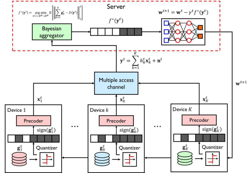
In this section, we describe learning and communication models for a wireless FL system. The wireless FL system consists of KK mobile devices and a server (or a base station) as depicted in Fig. 1. The server trains a neural network with a large number of hyper-parameters 𝐰∈ℝM{\bf w}\in\mathbb{R}^{M} by communicating with KK mobile devices through a shared wireless channel.

II-A Loss function

Let 𝐳ki∈ℝd\mathbf{z}_{k}^{i}\in\mathbb{R}^{d} and rki∈ℝr_{k}^{i}\in\mathbb{R} be the iith pair of the training data example stored at mobile device k∈[K]k\in[K]. Assuming, device kk has NkN_{k} training examples, we define a set of training examples stored at device k∈[K]k\in[K] as 𝒟k={𝐳ki,rki}i=1Nk\mathcal{D}_{k}=\{\mathbf{z}_{k}^{i},r_{k}^{i}\}_{i=1}^{N_{k}}. Therefore, a total number of training examples for learning becomes N=∑k=1KNkN=\sum_{k=1}^{K}N_{k}. Given model parameter 𝐰∈ℝM{\bf w}\in\mathbb{R}^{M}, we define a loss function with training pair (𝐳ki,rki)(\mathbf{z}_{k}^{i},r_{k}^{i}) as ℓ⁡(𝐳ki,rki,𝐰):ℝM×ℝ→ℝ\ell\left(\mathbf{z}_{k}^{i},r_{k}^{i};{\bf w}\right):\mathbb{R}^{M}\times\mathbb{R}\rightarrow\mathbb{R}. This loss can be either a cross entropy or a mean-squared error function according to machine learning applications. Using the sample average, the local loss function of device kk is defined as

fk​(𝐰)=1Nk​∑i=1Nkℓ⁡(𝐳ki,rki,𝐰).\displaystyle f_{k}\left(\mathbf{w}\right)=\frac{1}{N_{k}}\sum_{i=1}^{N_{k}}\ell\left(\mathbf{z}_{k}^{i},r_{k}^{i};\mathbf{w}\right). (1)

Summing fk​(𝐰)f_{k}\left(\mathbf{w}\right) with weight NkN\frac{N_{k}}{N} for k∈[K]k\in[K], the global loss function is given by

F⁡(𝐰)=1N​∑k=1K∑i=1Nkℓ⁡(𝐳ki,rki,𝐰)=∑k=1KNkN​fk​(𝐰).\displaystyle F\left(\mathbf{w}\right)=\frac{1}{N}\sum_{k=1}^{K}\sum_{i=1}^{N_{k}}\ell\left(\mathbf{z}_{k}^{i},r_{k}^{i};\mathbf{w}\right)=\sum_{k=1}^{K}\frac{N_{k}}{N}f_{k}\left(\mathbf{w}\right). (2)

II-B Wireless federated learning via singSGD

The wireless FL system iteratively optimizes model parameter 𝐰{\bf w} over TT communication rounds. Each communication round comprises 1) gradient computation and compression, 2) uplink transmissions, 3) model update, and 4) downlink transmission.

1) Gradient computation and compression: In communication round t∈[T]t\in[T], mobile device k∈[K]k\in[K] first computes local gradient information. Let 𝐠kt≜∇fk​(𝐰t)\mathbf{g}_{k}^{t}\triangleq\nabla f_{k}\left(\mathbf{w}^{t}\right) be the local gradient evaluated using model knowledge 𝐰t{\bf w}^{t} and local data set 𝒟k\mathcal{D}_{k} for k∈[K]k\in[K]. Then, it compresses local gradient using one-bit quantizer to diminish the uplink communication cost as

𝐠^kt=𝗌𝗂𝗀𝗇⁡(𝐠kt),\displaystyle\mathbf{\hat{g}}_{k}^{t}={\sf sign}\left(\mathbf{g}_{k}^{t}\right), (3)

where 𝗌𝗂𝗀𝗇⁡(x)=1{\sf sign}(x)=1 for x≥0x\geq 0 and 𝗌𝗂𝗀𝗇⁡(x)=−1{\sf sign}(x)=-1 otherwise.

Refer to caption
Fig. 1: Illustration of the wireless signSGD framework, in which mobile devices jointly train a model over a shared multiple access channel.

2) Uplink communications with precoding via a MAC: After the compression, mobile device kk transmits binary vector 𝐠^kt\mathbf{\hat{g}}_{k}^{t} along with the precoding coefficient vkt∈ℝv_{k}^{t}\in\mathbb{R}.

𝐱kt=vkt​𝗌𝗂𝗀𝗇​(𝐠kt),\displaystyle{\bf x}_{k}^{t}=v_{k}^{t}{\sf sign}\left(\mathbf{g}_{k}^{t}\right), (4)

where the precoder vktv_{k}^{t} satisfies the average power constraint as

𝔼⁡[|vkt|2]≤P.\displaystyle\mathbb{E}\left[\left|v_{k}^{t}\right|^{2}\right]\leq P. (5)

This compressed and precoded gradient information is sent over a shared multiple access channel. We focus on the real part of the complex-baseband signal model for ease of exposition. Let hkt∈ℝh_{k}^{t}\in\mathbb{R} be the real part of the complex baseband channel fading coefficient from mobile device kk to the server at communication round tt. We consider a block fading channel model, in which hkth_{k}^{t} independently changes over different communication rounds, while it remains as a constant per communication round. Then, under the premise of perfect synchronization, the received signal is given by

𝐲t\displaystyle{\bf y}^{t} =∑k=1Khkt​𝐱kt+𝐧t,\displaystyle=\sum_{k=1}^{K}h_{k}^{t}{\bf x}_{k}^{t}+{\bf n}^{t}, (6)

where 𝐧t{\bf n}^{t} is the real part of the complex-baseband noise signal at the server, which is distributed as independent and identically distributed (IID) Gaussian, i.e., 𝐧t∼𝒩⁡(0,12​𝐈M){\bf n}^{t}\sim\mathcal{N}\left(0,\frac{1}{2}{\bf I}_{M}\right).

3) Model update: In communication round t∈[T]t\in[T], the server performs the update of the model parameter using the gradient descent algorithm [1]. To perform the gradient decent algorithm, the server requires to estimate the sum of local gradients from the received signal 𝐲t{\bf y}^{t}, which is a noisy version of the sum of faded local gradients. Let U⁡(⋅):ℝM→ℝMU(\cdot):\mathbb{R}^{M}\rightarrow\mathbb{R}^{M} be the sum gradient estimator. Then, the MSE-optimal gradient estimator is defined as

f⋆(𝐲t)=argminU⁡(⋅):ℝM→ℝM𝔼[‖∑k=1K𝐠kt−U(𝐲t)‖22].\displaystyle f^{\star}({\bf y}^{t})=\arg\min_{U(\cdot):\mathbb{R}^{M}\rightarrow\mathbb{R}^{M}}\mathbb{E}\left[\left\|\sum_{k=1}^{K}{\bf g}_{k}^{t}-U({\bf y}^{t})\right\|_{2}^{2}\right]. (7)

Using this MSE-optimal estimator, the server updates the model parameter with learning rate γt∈ℝ+\gamma^{t}\in\mathbb{R}^{+} at communication round tt for the next round iteration:

𝐰t+1=𝐰t−γt​f⋆​(𝐲t).\displaystyle\mathbf{w}^{t+1}=\mathbf{w}^{t}-\gamma^{t}f^{\star}({\bf y}^{t}). (8)
f𝖡𝖺𝗒𝖠𝗂𝗋𝖢𝗈𝗆𝗉​(ymt)\displaystyle f_{\sf{BayAirComp}}\left(y_{m}^{t}\right) =1K​∑k=1K[μkt+2π​νkt​∑𝐛∈ℬK,kexp⁡[−(ymt−(𝐡t)T​𝐛)22​σ2]−∑𝐛∈(ℬK,k)cexp⁡[−(ymt−(𝐡t)⊤​𝐛)22​σ2]∑𝐛∈ℬKexp⁡[−(ymt−(𝐡t)T​𝐛)22​σ2]].\displaystyle=\frac{1}{K}\sum_{k=1}^{K}\left[\mu_{k}^{t}+\sqrt{\frac{2}{\pi}}\nu_{k}^{t}\frac{\sum_{\mathbf{b}\in\mathcal{B}_{K,k}}\exp\left[-\frac{\left(y_{m}^{t}-\left(\mathbf{h}^{t}\right)^{T}\mathbf{b}\right)^{2}}{2\sigma^{2}}\right]-\sum_{\mathbf{b}\in\left(\mathcal{B}_{K,k}\right)^{c}}\exp\left[-\frac{\left(y_{m}^{t}-(\mathbf{h}^{t})^{\top}\mathbf{b}\right)^{2}}{2\sigma^{2}}\right]}{\sum_{\mathbf{b}\in\mathcal{B}_{K}}\exp\left[-\frac{\left(y_{m}^{t}-\left(\mathbf{h}^{t}\right)^{T}\mathbf{b}\right)^{2}}{2\sigma^{2}}\right]}\right].{} (9)


4) Downlink communication: Using the broadcast nature of the wireless medium, the server multicasts the updated model parameter 𝐰t+1\mathbf{w}^{t+1} to mobile devices using a shared downlink channel. We assume that all mobile devices can perfectly decode the updated model parameters over entire communication rounds for ease of exposition.

III BayAirComp with Sign-Alignment Precoding

In this section, we present a novel wireless federated learning algorithm. The key idea of the proposed algorithm entails two operations: 1) sign-alignment precoding in the uplink transmission and 2) the Bayesian AirComp aggregation in the reception.

III-A Local Gradient Parameter Estimation and Compression

To implement the Bayesian aggregation in [15], the server requires to know the prior distribution of local gradients 𝐠kt∈ℝM{\bf g}_{k}^{t}\in\mathbb{R}^{M}. Unfortunately, it is infeasible to characterize the exact prior distribution of 𝐠kt{\bf g}_{k}^{t} because it depends on both the local data distribution and deep neural network structures. Instead, we model the prior distribution of 𝐠kt{\bf g}_{k}^{t} as Gaussian with the moment matching technique [15]. Specifically, let gk,mtg_{k,m}^{t} be the mmth entry of 𝐠kt{\bf g}_{k}^{t}. We model that gk,mtg_{k,m}^{t} follows IID Gaussian with mean μkt\mu_{k}^{t} and variance (νkt)2\left(\nu_{k}^{t}\right)^{2}, i.e., gk,mt∼𝒩⁡(μkt,(νkt)2)g_{k,m}^{t}\sim\mathcal{N}(\mu_{k}^{t},\left(\nu_{k}^{t}\right)^{2}). The mean and variance are estimated by taking the sample average estimator as

μkt=1M​∑m=1Mgk,mt​and​(νkt)2=1M​∑m=1M(gk,mt−μkt)2.\displaystyle\mu_{k}^{t}=\frac{1}{M}\sum_{m=1}^{M}g_{k,m}^{t}~~{\rm and}~~\left(\nu_{k}^{t}\right)^{2}=\frac{1}{M}\sum_{m=1}^{M}\left(g_{k,m}^{t}-\mu_{k}^{t}\right)^{2}. (10)

Although this Gaussian approximation on the prior distribution is not exact, it not only allows the Bayesian aggregation computationally tractable but also improves learning performance when training CNNs using MNIST datasets [15] in an orthogonalized multiple access channel environment. After computing the moments, each device normalizes the local gradient by subtracting its mean:

g¯k,mt=gk,mt−μkt.\displaystyle\bar{g}_{k,m}^{t}=g_{k,m}^{t}-\mu_{k}^{t}. (11)

Afterwards, mobile device kk compresses the local gradient to diminish the uplink communication cost by using one-bit quantizer as

𝐠^kt=sign​(𝐠¯kt).\displaystyle\mathbf{\hat{g}}_{k}^{t}=\text{sign}\left(\mathbf{\bar{g}}_{k}^{t}\right). (12)

Mobile device k∈[K]k\in[K] sends 𝐠^kt∈{−1,+1}M\mathbf{\hat{g}}_{k}^{t}\in\{-1,+1\}^{M} with μkt∈ℝ+\mu_{k}^{t}\in\mathbb{R}^{+} and νkt∈ℝ+\nu_{k}^{t}\in\mathbb{R}^{+} to the server.

III-B Sign-alignment precoding

When sending compressed local gradient, 𝐠^kt\mathbf{\hat{g}}_{k}^{t}, device kk requires to use precoder to compensate for the effect of wireless fading hkth_{k}^{t}. Unlike the prior approaches to invert the fading coefficient for precoding, we take a novel precoding strategy that requires one-bit CSI feedback from the BS. Our proposed precoding strategy is to align the signs of local gradients using one-bit precoding, i.e., vkt=𝗌𝗂𝗀𝗇⁡(hkt)v_{k}^{t}={\sf sign}(h_{k}^{t}) as

𝐱k=𝗌𝗂𝗀𝗇⁡(hkt)​𝐠^kt.\displaystyle{\bf x}_{k}={\sf sign}(h_{k}^{t}){\bf\hat{g}}_{k}^{t}. (13)

The received signal at the BS becomes

𝐲t\displaystyle{\bf y}^{t} =∑k=1K|hkt|​𝐠^kt+𝐧t.\displaystyle=\sum_{k=1}^{K}|h_{k}^{t}|{\bf\hat{g}}_{k}^{t}+{\bf n}^{t}. (14)

This precoding strategy ensures to align the signs of local gradients. This sign alignment effect helps to estimate the sum-gradient accurately by avoiding the sign flipping errors due to the wireless channel fadings. In addition, this precoding strategy requires only one-bit CSI overhead compared to the conventional precoding system which needs 6∼126\sim 12 bits for full CSI. Therefore, high efficiency can be obtained through this precoding strategy.

Refer to caption
Fig. 2: Comparison of aggregation functions according to fading coefficients and SNRs.

III-C Bayesian AirComp

Using received signal 𝐲t{\bf y}^{t}, the BS requires estimating the sum of local gradients ∑k=1K𝐠kt\sum_{k=1}^{K}{\bf g}_{k}^{t} to accomplish the model update via a stochastic gradient descent algorithm. We present a novel aggregation method called BayAirComp. The key idea of BayAirComp is to estimate the sum of local gradients ∑k=1K𝐠kt\sum_{k=1}^{K}{\bf g}_{k}^{t} by jointly exploiting the knowledge of the prior distribution of 𝐠kt{\bf g}_{k}^{t} (i.e., μkt\mu_{k}^{t} and νkt\nu_{k}^{t}), one-bit quantizer, and fading coefficient hkth_{k}^{t} to minimize the MSE. The aggregation function for BayAirComp f𝖡𝖺𝗒𝖠𝗂𝗋𝖢𝗈𝗆𝗉​(ymt):ℝ→ℝf_{\sf{BayAirComp}}(y_{m}^{t}):\mathbb{R}\rightarrow\mathbb{R} aims to minimize MSE, i.e.,

f𝖡𝖺𝗒𝖠𝗂𝗋𝖢𝗈𝗆𝗉(ymt)=argminf:ℝ→ℝ𝔼[|f(ymt)−∑k=1Kgk,mt|2].\displaystyle f_{\sf{BayAirComp}}(y_{m}^{t})=\arg\min_{f:\mathbb{R}\rightarrow\mathbb{R}}\mathbb{E}\left[\left|f(y_{m}^{t})-\sum_{k=1}^{K}g_{k,m}^{t}\right|^{2}\right]. (15)

The following theorem suggests the aggregation function for BayAirComp in closed form.

Theorem 1.

Let 𝐡t=[|h1t|,|h2t|,⋯,|hKt|]∈ℝ+K\mathbf{h}^{t}=\left[|h_{1}^{t}|,|h_{2}^{t}|,\cdots,|h_{K}^{t}|\right]\in\mathbb{R}_{+}^{K} be the sign-aligned channel vector at communication round tt. We also denote ℬK={−1,1}K\mathcal{B}_{K}=\{-1,1\}^{K} be a set with 2K2^{K} elements of binary vectors with length KK, i.e., 𝐛∈ℬK{\bf b}\in\mathcal{B}_{K}. We also define a subset ℬK,k⊂ℬK\mathcal{B}_{K,k}\subset\mathcal{B}_{K} that contains binary vectors whose kkth component is fixed to one. Then, the BayAirComp aggregation function is given by (9).

Proof.

From the Bayesian principle, the MSE-optimal aggregation function is obtained by computing the conditional expectation as

argminf:ℝ→ℝ𝔼[|f(ymt)−∑k=1Kg¯k,mt|2]\displaystyle\arg\underset{f:\mathbb{R}\rightarrow\mathbb{R}}{\min}\mathbb{E}\left[\left|f\left(y_{m}^{t}\right)-\sum_{k=1}^{K}\bar{g}_{k,m}^{t}\right|^{2}\right] =𝔼[∑k=1Kg¯k,mt|ymt]\displaystyle=\mathbb{E}\left[\left.\sum_{k=1}^{K}\bar{g}_{k,m}^{t}\right|y_{m}^{t}\right]
=∑k=1K𝔼⁡[g¯k,mt|ymt],\displaystyle=\sum_{k=1}^{K}\mathbb{E}\left[\bar{g}_{k,m}^{t}\middle|y_{m}^{t}\right],{} (16)

where the last equality is the linearity of the expectation. The conditional expectation in (16) is computed as

𝔼[g¯k,mt|ymt]=∫−∞∞g¯k,mtP(ymt|g¯k,mt)P(g¯k,mt)dg¯k,mt∫−∞∞P(ymt|g¯k,mt)P(g¯k,mt)dg¯k,mt.\displaystyle\mathbb{E}\left[\left.\bar{g}_{k,m}^{t}\right|y_{m}^{t}\right]=\frac{\int_{-\infty}^{\infty}\bar{g}_{k,m}^{t}P\left(\left.y_{m}^{t}\right|\bar{g}_{k,m}^{t}\right)P\left(\bar{g}_{k,m}^{t}\right)\,d\bar{g}_{k,m}^{t}}{\int_{-\infty}^{\infty}P\left(\left.y_{m}^{t}\right|\bar{g}_{k,m}^{t}\right)P\left(\bar{g}_{k,m}^{t}\right)\,d\bar{g}_{k,m}^{t}}. (17)

We define 𝐠~mt=[g¯1,mt,g¯2,mt,⋯,g¯K,mt]{\bf\tilde{g}}_{m}^{t}=[\bar{g}_{1,m}^{t},\bar{g}_{2,m}^{t},\cdots,\bar{g}_{K,m}^{t}]. Applying the one-bit precoding for the sign alignment, the channel likelihood distribution is

P(ymt|gm,1t,…,gm,Kt)=12​π​σ2e−(ymt−∑k=1K|hkt|​𝗌𝗂𝗀𝗇​(g¯k,mt))22​σ2.\displaystyle P\!\left(\left.y_{m}^{t}\right|{g}_{m,1}^{t},\ldots,{g}_{m,K}^{t}\right)=\frac{1}{\sqrt{2\pi\sigma^{2}}}e^{-\frac{\left(y_{m}^{t}-\sum_{k=1}^{K}|h_{k}^{t}|{\sf sign}\left(\bar{g}_{k,m}^{t}\right)\right)^{2}}{2\sigma^{2}}}. (18)

To obtain P(ymt|g¯m,kt)P\!\left(\left.y_{m}^{t}\right|{\bar{g}}_{m,k}^{t}\right), we need to marginalize (18) with respect to g¯m,1t,…,g¯m,k−1t,g¯m,k+1t,…,g¯m,Kt{\bar{g}}_{m,1}^{t},\ldots,{\bar{g}}_{m,k-1}^{t},{\bar{g}}_{m,k+1}^{t},\ldots,{\bar{g}}_{m,K}^{t}, where g¯k,mt∼𝒩⁡(0,(νkt)2){\bar{g}}_{k,m}^{t}\sim\mathcal{N}\left(0,\left(\nu_{k}^{t}\right)^{2}\right). Then, the marginal distribution P(ymt|gm,kt)P\!\left(\left.y_{m}^{t}\right|{g}_{m,k}^{t}\right), we compute the numerator in (17) as

∫−∞∞g¯k,mtP(ymt|g¯k,mt)P(g¯k,mt)dg¯k,mt\displaystyle\int_{-\infty}^{\infty}\bar{g}_{k,m}^{t}P\left(\left.y_{m}^{t}\right|\bar{g}_{k,m}^{t}\right)P\left(\bar{g}_{k,m}^{t}\right)\,d\bar{g}_{k,m}^{t}
=12K−1​2​π​σ22πνkt[∑𝐛∈ℬK,kexp{−(ymt−(𝐡t)⊤​𝐛)22​σz2}\displaystyle=\frac{1}{2^{K-1}\sqrt{2\pi\sigma^{2}}}\sqrt{\frac{2}{\pi}}\nu_{k}^{t}\left[\sum_{\mathbf{b}\in\mathcal{B}_{K,k}}\exp\left\{-\frac{\left(y_{m}^{t}-(\mathbf{h}^{t})^{\top}\mathbf{b}\right)^{2}}{2\sigma_{z}^{2}}\right\}\right.
−∑𝐛∈ℬK,kcexp{−(ymt−(𝐡t)⊤​𝐛)22​σz2}],\displaystyle~~~~~~~~~~~~~~~~~~~~~~~~~\left.-\sum_{\mathbf{b}\in\mathcal{B}_{K,k}^{c}}\exp\left\{-\frac{\left(y_{m}^{t}-(\mathbf{h}^{t})^{\top}\mathbf{b}\right)^{2}}{2\sigma_{z}^{2}}\right\}\right],{} (19)

and

∫−∞∞P(ymt|g¯k,mt)P(g¯k,mt)dg¯k,mt\displaystyle\int_{-\infty}^{\infty}P\left(\left.y_{m}^{t}\right|\bar{g}_{k,m}^{t}\right)P\left(\bar{g}_{k,m}^{t}\right)\,d\bar{g}_{k,m}^{t}
=12K−1​2​π​σ2​∑𝐛∈ℬKexp⁡{−(ymt−(𝐡t)⊤​𝐛)22​σ2}.\displaystyle=\frac{1}{2^{K-1}\sqrt{2\pi\sigma^{2}}}\sum_{\mathbf{b}\in\mathcal{B}^{K}}\exp\left\{-\frac{\left(y_{m}^{t}-(\mathbf{h}^{t})^{\top}\mathbf{b}\right)^{2}}{2\sigma^{2}}\right\}.{} (20)

The estimated gradient of the kkth device is derived by substituting (19) and (20) for (17), which arrives at the expression in (9). ∎

It is instructive to consider special cases for a better understanding of the proposed aggregation function for BayAirComp.

Example: Suppose K=5K=5. We first assume that all channel fading coefficients are identical in the magnitude |hkt|=1|h_{k}^{t}|=1 for k∈[K]k\in[K]. In this case, as depicted in Fig. 2 (left-side), the aggregation function becomes a uniform soft-step function with maximum and minimum values of ±2π\pm\sqrt{\frac{2}{\pi}}. As SNR increases, the soft-step function tends to be sharp. In a heterogeneous fading environment, |h1|=5|h_{1}|=5 and |hk|=1|h_{k}|=1 for k∈{2,3,4,5}k\in\{2,3,4,5\}, the proposed aggregation function plays a role of a non-uniform quantizer as illustrated in depicted in Fig. 2 (right-side). As depicted in Fig. 2-(a), our proposed BayAirComp clearly differs from the majority-voting based aggregation function. The proposed BayAirComp provides the magnitude information of g¯k,mt{\bar{g}}_{k,m}^{t} in a quantized manner. Whereas, the majority-voting based aggregation keeps the sign of g¯k,mt{\bar{g}}_{k,m}^{t}.

Remark (Implementation): To implement BayAirComp, mobile device k∈[K]k\in[K] requires to additionally send μkt∈ℝ\mu_{k}^{t}\in\mathbb{R} and νkt∈ℝ+\nu_{k}^{t}\in\mathbb{R}^{+} to the server per communication round. As shown in our prior work [15], this information can be quantized with BB-bit scalar quantizer and be transmitted to the server using orthogonal resources. Since this additional information bits are much smaller than the model size M∼106M\sim 10^{6}, i.e.,2​B≪M2B\ll M, the additional overheads can be negligible.

IV Performance Analysis

In this section, we provide the convergence analysis of the proposed FL algorithm in this paper. The analysis procedure is carried out in two steps. First, obtain the MSE bound between the true gradient and the gradient estimate by the aggregation function, and then show the gradient of the SGD-based FL algorithm converges to zero. The convergence proof is under the assumption that the global loss function F⁡(𝐰)F\left(\mathbf{w}\right) is LL-Lipschitz smooth and has the least value in 𝐰∗\mathbf{w}^{*}. For ease of expression, let define 𝐠𝗍𝗋𝗎𝖾t=∇F​(𝐰t)=1K​∑k=1K𝐠kt\mathbf{g}_{\mathsf{true}}^{t}=\nabla F\left(\mathbf{w}^{t}\right)=\frac{1}{K}\sum_{k=1}^{K}\mathbf{g}_{k}^{t}.

IV-A MSE Bound

Theorem 2.

Let gk,mtg_{k,m}^{t} be an IID Gaussian with mean μkt\mu_{k}^{t} and variance (νkt)2\left(\nu_{k}^{t}\right)^{2}, i.e. gk,mt∼𝒩⁡(μkt,(νkt)2)g_{k,m}^{t}\sim\mathcal{N}\left(\mu_{k}^{t},\left(\nu_{k}^{t}\right)^{2}\right), for k∈[K]k\in\left[K\right] and m∈[M]m\in\left[M\right]. For the error 𝐞t=f𝖡𝖺𝗒𝖠𝗂𝗋𝖢𝗈𝗆𝗉​(𝐲t)−𝐠𝗍𝗋𝗎𝖾t\mathbf{e}^{t}=f_{\mathsf{BayAirComp}}\left(\mathbf{y}^{t}\right)-\mathbf{g}_{\mathsf{true}}^{t} , the MSE bound σ𝖬𝖲𝖤2≥𝔼⁡[∥𝐞t∥22]\sigma_{\mathsf{MSE}}^{2}\geq\mathbb{E}\left[\lVert\mathbf{e}^{t}\rVert_{2}^{2}\right] can be expressed as

σ𝖬𝖲𝖤2=MK2​(1+2π)​∑k=1K(νkt)2.\displaystyle\sigma_{\mathsf{MSE}}^{2}=\frac{M}{K^{2}}\left(1+\frac{2}{\pi}\right)\sum_{k=1}^{K}\left(\nu_{k}^{t}\right)^{2}. (21)
Proof.

To reduce the complexity of expressing formulas, we simplify (9) as

f𝖡𝖺𝗒𝖠𝗂𝗋𝖢𝗈𝗆𝗉​(ymt)=1K​∑k=1K[μkt+νkt​2π​Ak​(ymt)].\displaystyle f_{\mathsf{BayAirComp}}\left(y_{m}^{t}\right)=\frac{1}{K}\sum_{k=1}^{K}\left[\mu_{k}^{t}+\nu_{k}^{t}\sqrt{\frac{2}{\pi}}A_{k}\!\left(y_{m}^{t}\right)\right]. (22)

Putting the aggregation function into the gradient error definition, we can obtain the formula as

1K​∑k=1K[μkt+νkt​2π​Ak​(ymt)]\displaystyle\frac{1}{K}\sum_{k=1}^{K}\left[\mu_{k}^{t}+\nu_{k}^{t}\sqrt{\frac{2}{\pi}}A_{k}\!\left(y_{m}^{t}\right)\right] =1K​∑k=1Kgk,mt+emt\displaystyle=\frac{1}{K}\sum_{k=1}^{K}g_{k,m}^{t}+e_{m}^{t}
=1K​∑k=1K[gk,mt+ek,mt],\displaystyle=\frac{1}{K}\sum_{k=1}^{K}\left[g_{k,m}^{t}+e_{k,m}^{t}\right],{} (23)

where (23) is for the mmth component of gradient, and ek,mte_{k,m}^{t} is the error for the kkth device in emte_{m}^{t}. Then, we compute the MSE bound as follows.

𝔼⁡[∥𝐞t∥22]\displaystyle\mathbb{E}\left[\lVert\mathbf{e}^{t}\rVert_{2}^{2}\right] =𝔼⁡[∑m=1M|emt|2]\displaystyle=\mathbb{E}\left[\sum_{m=1}^{M}\lvert e_{m}^{t}\rvert^{2}\right]
=∑m=1M𝔼⁡[|emt|2]\displaystyle=\sum_{m=1}^{M}\mathbb{E}\left[\lvert e_{m}^{t}\rvert^{2}\right]
=∑m=1M𝔼⁡[|1K​∑k=1Kek,mt|2]\displaystyle=\sum_{m=1}^{M}\mathbb{E}\left[\left|\frac{1}{K}\sum_{k=1}^{K}e_{k,m}^{t}\right|^{2}\right]
≤∑k=1K𝔼⁡[1K2​∑k=1K|ek,mt|2]\displaystyle\leq\sum_{k=1}^{K}\mathbb{E}\left[\frac{1}{K^{2}}\sum_{k=1}^{K}\left|e_{k,m}^{t}\right|^{2}\right]
=1K2​∑m=1M∑k=1K𝔼⁡[|ek,mt|2].\displaystyle=\frac{1}{K^{2}}\sum_{m=1}^{M}\sum_{k=1}^{K}\mathbb{E}\left[\left|e_{k,m}^{t}\right|^{2}\right].{} (24)

The inequality in (24) is reasonable according to the convexity. Using the assumption that the local gradients gk,mtg_{k,m}^{t} and g¯k,mt\bar{g}_{k,m}^{t} is IID Gaussian, it is possible to compute the upper bound of MSE as below.

𝔼⁡[∥𝐞t∥22]\displaystyle\mathbb{E}\left[\lVert\mathbf{e}^{t}\rVert_{2}^{2}\right]
≤1K2​∑m=1M∑k=1K𝔼⁡[|gk,mt−μkt−νkt​2π​Ak​(ymt)|2]\displaystyle\leq\frac{1}{K^{2}}\sum_{m=1}^{M}\sum_{k=1}^{K}\mathbb{E}\left[\left|g_{k,m}^{t}-\mu_{k}^{t}-\nu_{k}^{t}\sqrt{\frac{2}{\pi}}A_{k}\!\left(y_{m}^{t}\right)\right|^{2}\right]
=1K2​∑m=1M∑k=1K𝔼⁡[|g¯k,mt−νkt​2π​Ak​(ymt)|2]\displaystyle=\frac{1}{K^{2}}\sum_{m=1}^{M}\sum_{k=1}^{K}\mathbb{E}\left[\left|\bar{g}_{k,m}^{t}-\nu_{k}^{t}\sqrt{\frac{2}{\pi}}A_{k}\!\left(y_{m}^{t}\right)\right|^{2}\right]
=1K2​∑m=1M∑k=1K𝔼g¯k,mt​[|g¯k,mt−νkt​2π​𝔼ymt​[Ak​(ymt)]|2]\displaystyle=\frac{1}{K^{2}}\!\sum_{m=1}^{M}\sum_{k=1}^{K}\mathbb{E}_{\bar{g}_{k,m}^{t}}\!\!\!\left[\left|\bar{g}_{k,m}^{t}-\nu_{k}^{t}\sqrt{\frac{2}{\pi}}\mathbb{E}_{y_{m}^{t}}\!\!\left[A_{k}\!\left(y_{m}^{t}\right)\right]\right|^{2}\right]
≤1K2​∑m=1M∑k=1K[V​a​r​(gk,mt)+2π​(νkt)2]\displaystyle\leq\frac{1}{K^{2}}\sum_{m=1}^{M}\sum_{k=1}^{K}\left[Var\left(g_{k,m}^{t}\right)+\frac{2}{\pi}\left(\nu_{k}^{t}\right)^{2}\right]
=1K2​∑m=1M∑k=1K(1+2π)​(νkt)2.\displaystyle=\frac{1}{K^{2}}\sum_{m=1}^{M}\sum_{k=1}^{K}\left(1+\frac{2}{\pi}\right)\left(\nu_{k}^{t}\right)^{2}.{} (25)

The inequality in (25) is due to the property that

𝔼𝐗​[(𝐗−a)2]\displaystyle\mathbb{E}_{\mathbf{X}}\left[\left(\mathbf{X}-a\right)^{2}\right] =σ𝐗2+(μ𝐗−a)2\displaystyle=\sigma_{\mathbf{X}}^{2}+\left(\mu_{\mathbf{X}}-a\right)^{2}
≤σ𝐗2+maxa⁡(μ𝐗−a)2,\displaystyle\leq\sigma_{\mathbf{X}}^{2}+\max_{a}\left(\mu_{\mathbf{X}}-a\right)^{2},{} (26)

and −1<Ak​(ymt)<1-1<A_{k}\!\left(y_{m}^{t}\right)<1 regardless of ymty_{m}^{t}. Therefore the upper bound of MSE σ𝖬𝖲𝖤2\sigma_{\mathsf{MSE}}^{2} in (21) can be achieved. ∎

IV-B Convergence Analysis

Theorem 3.

For the LL-Lipschitz smooth loss function F⁡(𝐰)F\left(\mathbf{w}\right), the proposed FL algorithm with the learning rate γt=γt+1\gamma^{t}=\frac{\gamma}{t+1} for γ>0\gamma>0 satisfies

𝔼⁡[1T​∑t=0T∥𝐠𝗍𝗋𝗎𝖾t∥22]\displaystyle\mathbb{E}\left[\frac{1}{T}\sum_{t=0}^{T}\lVert\mathbf{g}_{\mathsf{true}}^{t}\rVert_{2}^{2}\right]
≤1T​[F⁡(𝐰0)−F⁡(𝐰∗)γ⁡(1−L​γ2)+σ𝖬𝖲𝖤2​(1+ln⁡T)​L​γ21−L​γ2].\displaystyle\leq\frac{1}{\sqrt{T}}\left[\frac{F\left(\mathbf{w}^{0}\right)-F\left(\mathbf{w}^{*}\right)}{\gamma\left(1-\frac{L\gamma}{2}\right)}+\sigma_{\mathsf{MSE}}^{2}\left(1+\ln T\right)\frac{\frac{L\gamma}{2}}{1-\frac{L\gamma}{2}}\right].{} (27)
Proof.

The proposed FL algorithm is based on GD, and the model parameter update formula is given as

𝐰t+1=𝐰t−γt​f𝖡𝖺𝗒𝖠𝗂𝗋𝖢𝗈𝗆𝗉​(𝐲t).\displaystyle\mathbf{w}^{t+1}=\mathbf{w}^{t}-\gamma^{t}f_{\mathsf{BayAirComp}}\left(\mathbf{y}^{t}\right). (28)

Since the loss function is LL-smooth, the convergence formula can be derived as

F⁡(𝐰t+1)\displaystyle F\left(\mathbf{w}^{t+1}\right)
≤F⁡(𝐰t)+(𝐠𝗍𝗋𝗎𝖾t)T​(𝐰t+1−𝐰t)+L2​∥𝐰t+1−𝐰t∥22\displaystyle\leq F\left(\mathbf{w}^{t}\right)+\left(\mathbf{g}_{\mathsf{true}}^{t}\right)^{T}\left(\mathbf{w}^{t+1}-\mathbf{w}^{t}\right)+\frac{L}{2}\lVert\mathbf{w}^{t+1}-\mathbf{w}^{t}\rVert_{2}^{2}
=F⁡(𝐰t)−(𝐠𝗍𝗋𝗎𝖾t)T​γt​f𝖡𝖺𝗒𝖠𝗂𝗋𝖢𝗈𝗆𝗉​(𝐲t)\displaystyle=F\left(\mathbf{w}^{t}\right)-\left(\mathbf{g}_{\mathsf{true}}^{t}\right)^{T}\gamma^{t}f_{\mathsf{BayAirComp}}\left(\mathbf{y}^{t}\right)
+L2​(γt)2​∥f𝖡𝖺𝗒𝖠𝗂𝗋𝖢𝗈𝗆𝗉​(𝐲t)∥22\displaystyle\hskip 120.00018pt+\frac{L}{2}\left(\gamma^{t}\right)^{2}\lVert f_{\mathsf{BayAirComp}}\left(\mathbf{y}^{t}\right)\rVert_{2}^{2}
=F⁡(𝐰t)−γt​(𝐠𝗍𝗋𝗎𝖾t)T​(𝐠𝗍𝗋𝗎𝖾t+𝐞t)+L2​(γt)2​∥𝐠𝗍𝗋𝗎𝖾t+𝐞t∥22,\displaystyle=F\left(\mathbf{w}^{t}\right)-\gamma^{t}\!\left(\mathbf{g}_{\mathsf{true}}^{t}\right)^{T}\!\left(\mathbf{g}_{\mathsf{true}}^{t}+\mathbf{e}^{t}\right)+\frac{L}{2}\left(\gamma^{t}\right)^{2}\!\lVert\mathbf{g}_{\mathsf{true}}^{t}+\mathbf{e}^{t}\rVert_{2}^{2},{} (29)

where the last equation is obtained by the gradient error definition. By taking the expectation in (29), we can derive

𝔼⁡[F⁡(𝐰t+1)−F⁡(𝐰t)]\displaystyle\mathbb{E}\left[F\left(\mathbf{w}^{t+1}\right)-F\left(\mathbf{w}^{t}\right)\right]
≤−(γt−L2​(γt)2)​𝔼​[∥𝐠𝗍𝗋𝗎𝖾t∥22]\displaystyle\leq-\left(\gamma^{t}-\frac{L}{2}\left(\gamma^{t}\right)^{2}\right)\mathbb{E}\left[\lVert\mathbf{g}_{\mathsf{true}}^{t}\rVert_{2}^{2}\right]
−(γt−L​(γt)2)​𝔼​[(𝐠𝗍𝗋𝗎𝖾t)T​𝐞t]+L2​(γt)2​𝔼​[∥𝐞t∥22].\displaystyle\hskip 11.00008pt-\left(\gamma^{t}-L\left(\gamma^{t}\right)^{2}\right)\mathbb{E}\left[\left(\mathbf{g}_{\mathsf{true}}^{t}\right)^{T}\mathbf{e}^{t}\right]+\frac{L}{2}\left(\gamma^{t}\right)^{2}\mathbb{E}\left[\lVert\mathbf{e}^{t}\rVert_{2}^{2}\right].{} (30)

Usually the learning rate γt<1\gamma^{t}<1, it seems reasonable that γt−L​(γt)2>0\gamma^{t}-L\left(\gamma^{t}\right)^{2}>0. To continue the convergence analysis, we should find the lower bound of 𝔼⁡[(𝐠𝗍𝗋𝗎𝖾t)T​𝐞t]\mathbb{E}\left[\left(\mathbf{g}_{\mathsf{true}}^{t}\right)^{T}\mathbf{e}^{t}\right].

Corollary: If the components of true gradient is Gaussian with mean μ𝗍𝗋𝗎𝖾t\mu_{\mathsf{true}}^{t} and variance (ν𝗍𝗋𝗎𝖾t)2\left(\nu_{\mathsf{true}}^{t}\right)^{2}, i.e. g𝗍𝗋𝗎𝖾,mt∼(μ𝗍𝗋𝗎𝖾t,(ν𝗍𝗋𝗎𝖾t)2)g_{\mathsf{true},m}^{t}\sim\left(\mu_{\mathsf{true}}^{t},\left(\nu_{\mathsf{true}}^{t}\right)^{2}\right) where m∈[M]m\in\left[M\right], 𝔼⁡[(𝐠𝗍𝗋𝗎𝖾t)T​𝐞t]\mathbb{E}\left[\left(\mathbf{g}_{\mathsf{true}}^{t}\right)^{T}\mathbf{e}^{t}\right] has a positive value in 𝖲𝖭𝖱→0\mathsf{SNR}\rightarrow 0 and 𝖲𝖭𝖱→∞\mathsf{SNR}\rightarrow\infty.

Proof.

Firstly, we can derive the mean and variance of g𝗍𝗋𝗎𝖾,mtg_{\mathsf{true},m}^{t} as

μ𝗍𝗋𝗎𝖾t=𝔼⁡[g𝗍𝗋𝗎𝖾,mt]=𝔼⁡[1K​∑k=1Kgk,mt]=1K​∑k=1Kμkt,\displaystyle\mu_{\mathsf{true}}^{t}=\mathbb{E}\left[g_{\mathsf{true},m}^{t}\right]=\mathbb{E}\left[\frac{1}{K}\sum_{k=1}^{K}g_{k,m}^{t}\right]=\frac{1}{K}\sum_{k=1}^{K}\mu_{k}^{t},{} (31)
(ν𝗍𝗋𝗎𝖾t)2=𝔼⁡[(g𝗍𝗋𝗎𝖾,mt−μ𝗍𝗋𝗎𝖾t)2]\displaystyle\!\left(\nu_{\mathsf{true}}^{t}\right)^{2}=\mathbb{E}\left[\left(g_{\mathsf{true},m}^{t}-\mu_{\mathsf{true}}^{t}\right)^{2}\right]
=𝔼⁡[(1K​∑k=1K(gk,mt−μkt))2]\displaystyle\hskip 31.0001pt=\mathbb{E}\left[\left(\frac{1}{K}\sum_{k=1}^{K}\left(g_{k,m}^{t}-\mu_{k}^{t}\right)\right)^{2}\right]
=𝔼⁡[1K2​∑k=1K(gk,mt−μkt)2]=1K2​∑k=1K(νkt)2.\displaystyle\hskip 32.00002pt=\mathbb{E}\left[\frac{1}{K^{2}}\sum_{k=1}^{K}\left(g_{k,m}^{t}-\mu_{k}^{t}\right)^{2}\right]=\frac{1}{K^{2}}\sum_{k=1}^{K}\left(\nu_{k}^{t}\right)^{2}.{} (32)

We can expressed 𝔼⁡[(𝐠𝗍𝗋𝗎𝖾t)T​𝐞t]\mathbb{E}\left[\left(\mathbf{g}_{\mathsf{true}}^{t}\right)^{T}\mathbf{e}^{t}\right] by summation of each component of the vector as below.

𝔼⁡[(𝐠𝗍𝗋𝗎𝖾t)T​𝐞t]\displaystyle\mathbb{E}\left[\left(\mathbf{g}_{\mathsf{true}}^{t}\right)^{T}\mathbf{e}^{t}\right]
=∑m=1M𝔼⁡[g𝗍𝗋𝗎𝖾,mt​(g𝗍𝗋𝗎𝖾,mt−f𝖡𝖺𝗒𝖠𝗂𝗋𝖢𝗈𝗆𝗉​(ymt))]\displaystyle=\sum_{m=1}^{M}\mathbb{E}\left[g_{\mathsf{true},m}^{t}\left(g_{\mathsf{true},m}^{t}-f_{\mathsf{BayAirComp}}\left(y_{m}^{t}\right)\right)\right]
=∑m=1M[𝔼[(g𝗍𝗋𝗎𝖾,mt)2]\displaystyle=\sum_{m=1}^{M}\left[\mathbb{E}\left[\left(g_{\mathsf{true},m}^{t}\right)^{2}\right]\right.
−𝔼[g𝗍𝗋𝗎𝖾,mt×1K∑k=1K(μkt+2πνktAk(ymt))]]\displaystyle\hskip 50.00008pt\left.-\mathbb{E}\left[g_{\mathsf{true},m}^{t}\times\frac{1}{K}\sum_{k=1}^{K}\left(\mu_{k}^{t}+\sqrt{\frac{2}{\pi}}\nu_{k}^{t}A_{k}\left(y_{m}^{t}\right)\right)\right]\right]
=∑m=1M[(ν𝗍𝗋𝗎𝖾t)2−2π​(1K​∑k=1Kνkt​𝔼​[g𝗍𝗋𝗎𝖾,mt​Ak​(ymt)])].\displaystyle=\sum_{m=1}^{M}\left[\left(\nu_{\mathsf{true}}^{t}\right)^{2}-\sqrt{\frac{2}{\pi}}\left(\frac{1}{K}\sum_{k=1}^{K}\nu_{k}^{t}\mathbb{E}\left[g_{\mathsf{true},m}^{t}A_{k}\left(y_{m}^{t}\right)\right]\right)\right].{} (33)

We consider about the exact value of 𝔼⁡[g𝗍𝗋𝗎𝖾,mt​Ak​(ymt)]\mathbb{E}\left[g_{\mathsf{true},m}^{t}A_{k}\left(y_{m}^{t}\right)\right] in two 𝖲𝖭𝖱\mathsf{SNR} cases to obtain 𝔼⁡[(𝐠𝗍𝗋𝗎𝖾t)T​𝐞t]\mathbb{E}\left[\left(\mathbf{g}_{\mathsf{true}}^{t}\right)^{T}\mathbf{e}^{t}\right]: 𝖲𝖭𝖱→0\mathsf{SNR}\rightarrow 0, and 𝖲𝖭𝖱→∞\mathsf{SNR}\rightarrow\infty.

1) 𝐒𝐍𝐑→𝟎\mathsf{\bf{SNR}}\rightarrow\bf{0} : In this case, the all exponential terms in (9) goes to one as the noise variance σ2\sigma^{2} goes to infinity, hence Ak​(ymt)=0A_{k}\left(y_{m}^{t}\right)=0. This derives 𝔼⁡[g𝗍𝗋𝗎𝖾,mt​Ak​(ymt)]=0\mathbb{E}\left[g_{\mathsf{true},m}^{t}A_{k}\left(y_{m}^{t}\right)\right]=0, so 𝔼⁡[(𝐠𝗍𝗋𝗎𝖾t)T​𝐞t]=M​(ν𝗍𝗋𝗎𝖾t)2>0\mathbb{E}\left[\left(\mathbf{g}_{\mathsf{true}}^{t}\right)^{T}\mathbf{e}^{t}\right]=M\left(\nu_{\mathsf{true}}^{t}\right)^{2}>0 can be achieved in (IV-B).

2) 𝐒𝐍𝐑→∞\mathsf{\bf{SNR}}\rightarrow\bf{\infty} : The additive noise is assumed to be zero, so the only one exponential term where 𝐛\mathbf{b} got the whole correct signs of users’ gradients is non-zero, and the others are zeros in (9). Therefore we can obtain Ak​(ymt)=𝗌𝗂𝗀𝗇⁡(g¯k,mt)A_{k}\left(y_{m}^{t}\right)=\mathsf{sign}\left(\bar{g}_{k,m}^{t}\right). Using this, we can represent the value of 𝔼⁡[g𝗍𝗋𝗎𝖾,𝗆t​Ak​(ymt)]\mathbb{E}\left[g_{\mathsf{true,m}}^{t}A_{k}\left(y_{m}^{t}\right)\right] as

𝔼⁡[g𝗍𝗋𝗎𝖾,𝗆t​Ak​(ymt)]\displaystyle\mathbb{E}\left[g_{\mathsf{true,m}}^{t}A_{k}\left(y_{m}^{t}\right)\right]
=𝔼⁡[1K​∑ℓ=1Kgℓ,mt​𝗌𝗂𝗀𝗇​(g¯k,mt)]\displaystyle=\mathbb{E}\left[\frac{1}{K}\sum_{\ell=1}^{K}g_{\ell,m}^{t}\mathsf{sign}\left(\bar{g}_{k,m}^{t}\right)\right]
=1K​[𝔼⁡[gk,mt​𝗌𝗂𝗀𝗇​(g¯k,mt)]+∑ℓ≠k𝔼⁡[gℓ,mt​𝗌𝗂𝗀𝗇​(g¯k,mt)]].\displaystyle=\frac{1}{K}\left[\mathbb{E}\left[g_{k,m}^{t}\mathsf{sign}\left(\bar{g}_{k,m}^{t}\right)\right]+\sum_{\ell\neq k}\mathbb{E}\left[g_{\ell,m}^{t}\mathsf{sign}\left(\bar{g}_{k,m}^{t}\right)\right]\right].{} (34)

We already know that gk,mtg_{k,m}^{t} and gℓ,mt​(ℓ≠k)g_{\ell,m}^{t}\left(\ell\neq k\right) are independent, so g¯k,mt\bar{g}_{k,m}^{t} and gℓ,mtg_{\ell,m}^{t} are also independent. By the property that 𝔼⁡[𝐗⋅f⁡(𝐘)]=𝔼⁡[𝐗]⋅𝔼⁡[f⁡(𝐘)]\mathbb{E}\left[\mathbf{X}\cdot f\left(\mathbf{Y}\right)\right]=\mathbb{E}\left[\mathbf{X}\right]\cdot\mathbb{E}\left[f\left(\mathbf{Y}\right)\right] where 𝐗\mathbf{X} and 𝐘\mathbf{Y} are independent, ∑ℓ≠k𝔼⁡[gℓ,mt​𝗌𝗂𝗀𝗇​(g¯k,mt)]=0\sum_{\ell\neq k}\mathbb{E}\left[g_{\ell,m}^{t}\mathsf{sign}\left(\bar{g}_{k,m}^{t}\right)\right]=0 since 𝔼⁡[𝗌𝗂𝗀𝗇⁡(g¯k,mt)]=0\mathbb{E}\left[\mathsf{sign}\left(\bar{g}_{k,m}^{t}\right)\right]=0. This helps to obtain the value of 𝔼⁡[g𝗍𝗋𝗎𝖾,𝗆t​Ak​(ymt)]\mathbb{E}\left[g_{\mathsf{true,m}}^{t}A_{k}\left(y_{m}^{t}\right)\right] as

𝔼⁡[g𝗍𝗋𝗎𝖾,𝗆t​Ak​(ymt)]\displaystyle\mathbb{E}\left[g_{\mathsf{true,m}}^{t}A_{k}\left(y_{m}^{t}\right)\right] =1K​𝔼​[gk,mt​𝗌𝗂𝗀𝗇​(g¯k,mt)]\displaystyle=\frac{1}{K}\mathbb{E}\left[g_{k,m}^{t}\mathsf{sign}\left(\bar{g}_{k,m}^{t}\right)\right]
=1K​𝔼​[(g¯k,mt+μkt)​𝗌𝗂𝗀𝗇​(g¯k,mt)]\displaystyle=\frac{1}{K}\mathbb{E}\left[\left(\bar{g}_{k,m}^{t}+\mu_{k}^{t}\right)\mathsf{sign}\left(\bar{g}_{k,m}^{t}\right)\right]
=1K​𝔼​[|g¯k,mt|]=1K​2π​νkt.\displaystyle=\frac{1}{K}\mathbb{E}\left[\left|\bar{g}_{k,m}^{t}\right|\right]=\frac{1}{K}\sqrt{\frac{2}{\pi}}\nu_{k}^{t}.{} (35)

Put this into (IV-B), we can get the exact value of 𝔼⁡[(𝐠𝗍𝗋𝗎𝖾t)T​𝐞t]\mathbb{E}\left[\left(\mathbf{g}_{\mathsf{true}}^{t}\right)^{T}\mathbf{e}^{t}\right] as

𝔼⁡[(𝐠𝗍𝗋𝗎𝖾t)T​𝐞t]\displaystyle\mathbb{E}\left[\left(\mathbf{g}_{\mathsf{true}}^{t}\right)^{T}\mathbf{e}^{t}\right]
=∑m=1M[(ν𝗍𝗋𝗎𝖾t)2−2π​(1K​∑k=1Kνkt⋅1K​2π​νkt)]\displaystyle=\sum_{m=1}^{M}\left[\left(\nu_{\mathsf{true}}^{t}\right)^{2}-\sqrt{\frac{2}{\pi}}\left(\frac{1}{K}\sum_{k=1}^{K}\nu_{k}^{t}\cdot\frac{1}{K}\sqrt{\frac{2}{\pi}}\nu_{k}^{t}\right)\right]
=∑m=1M[(ν𝗍𝗋𝗎𝖾t)2−2π​(1K2​∑k=1K(νkt)2)]\displaystyle=\sum_{m=1}^{M}\left[\left(\nu_{\mathsf{true}}^{t}\right)^{2}-\frac{2}{\pi}\left(\frac{1}{K^{2}}\sum_{k=1}^{K}\left(\nu_{k}^{t}\right)^{2}\right)\right]
=M⁡(1−2π)​(ν𝗍𝗋𝗎𝖾t)2>0.\displaystyle=M\left(1-\frac{2}{\pi}\right)\left(\nu_{\mathsf{true}}^{t}\right)^{2}>0.{} (36)

Consequently, we can summarize that

𝔼⁡[(𝐠𝗍𝗋𝗎𝖾t)T​𝐞t]={M​(ν𝗍𝗋𝗎𝖾t)2,𝖲𝖭𝖱→0M⁡(1−2π)​(ν𝗍𝗋𝗎𝖾t)2,𝖲𝖭𝖱→∞,\displaystyle\mathbb{E}\left[\left(\mathbf{g}_{\mathsf{true}}^{t}\right)^{T}\mathbf{e}^{t}\right]=\begin{cases}M\left(\nu_{\mathsf{true}}^{t}\right)^{2},&\mathsf{SNR}\rightarrow 0\\ M\left(1-\frac{2}{\pi}\right)\left(\nu_{\mathsf{true}}^{t}\right)^{2},&\mathsf{SNR}\rightarrow\infty\end{cases}, (37)

and all the values are positive. This completes the proof.

∎

According to the corollary, (IV-B) can be reduced in some particular cases as

𝔼⁡[F⁡(𝐰t+1−F⁡(𝐰t))]\displaystyle\mathbb{E}\left[F\left(\mathbf{w}^{t+1}-F\left(\mathbf{w}^{t}\right)\right)\right]
≤−(γt−L2​(γt)2)​𝔼​[∥𝐠𝗍𝗋𝗎𝖾t∥22]+L2​(γt)2​𝔼​[∥𝐞t∥22].\displaystyle\leq-\left(\gamma^{t}-\frac{L}{2}\left(\gamma^{t}\right)^{2}\right)\mathbb{E}\left[\lVert\mathbf{g}_{\mathsf{true}}^{t}\rVert_{2}^{2}\right]+\frac{L}{2}\left(\gamma^{t}\right)^{2}\mathbb{E}\left[\lVert\mathbf{e}^{t}\rVert_{2}^{2}\right].{} (38)

Using the result 𝔼⁡[∥𝐞t∥22]≤σ𝖬𝖲𝖤2\mathbb{E}\left[\lVert\mathbf{e}^{t}\rVert_{2}^{2}\right]\leq\sigma_{\mathsf{MSE}}^{2} and the adaptive learning rate γt=γt+1≤γt+1\gamma^{t}=\frac{\gamma}{t+1}\leq\frac{\gamma}{\sqrt{t+1}}, we can simplify (IV-B) as

𝔼⁡[F⁡(𝐰t+1)−F⁡(𝐰t)]\displaystyle\mathbb{E}\left[F\left(\mathbf{w}^{t+1}\right)-F\left(\mathbf{w}^{t}\right)\right]
≤−(γt+1−L2​γ2t+1)​𝔼​[∥𝐠𝗍𝗋𝗎𝖾t∥22]+L2​γ2t+1​σ𝖬𝖲𝖤2\displaystyle\leq-\left(\frac{\gamma}{\sqrt{t+1}}-\frac{L}{2}\frac{\gamma^{2}}{t+1}\right)\mathbb{E}\left[\lVert\mathbf{g}_{\mathsf{true}}^{t}\rVert_{2}^{2}\right]+\frac{L}{2}\frac{\gamma^{2}}{t+1}\sigma_{\mathsf{MSE}}^{2}
≤−γt+1​𝔼​[∥𝐠𝗍𝗋𝗎𝖾t∥22]​(1−L​γ2)+L2​γ2t+1​σ𝖬𝖲𝖤2.\displaystyle\leq-\frac{\gamma}{\sqrt{t+1}}\mathbb{E}\left[\lVert\mathbf{g}_{\mathsf{true}}^{t}\rVert_{2}^{2}\right]\left(1-\frac{L\gamma}{2}\right)+\frac{L}{2}\frac{\gamma^{2}}{t+1}\sigma_{\mathsf{MSE}}^{2}.{} (39)

If (39) is summed for all rounds t∈[T]t\in[T], it can be organized as

F⁡(𝐰0)−F⁡(𝐰∗)\displaystyle F\left(\mathbf{w}^{0}\right)-F\left(\mathbf{w}^{*}\right)
≥𝔼⁡[∑t=0T−1(F⁡(𝐰t)−F⁡(𝐰t+1))]\displaystyle\geq\mathbb{E}\left[\sum_{t=0}^{T-1}\left(F\left(\mathbf{w}^{t}\right)-F\left(\mathbf{w}^{t+1}\right)\right)\right]
≥∑t=0T−1[γt+1​𝔼​[∥𝐠𝗍𝗋𝗎𝖾t∥22]​(1−L​γ2)−L2​γ2t+1​σ𝖬𝖲𝖤2]\displaystyle\geq\sum_{t=0}^{T-1}\left[\frac{\gamma}{\sqrt{t+1}}\mathbb{E}\left[\lVert\mathbf{g}_{\mathsf{true}}^{t}\rVert_{2}^{2}\right]\left(1-\frac{L\gamma}{2}\right)-\frac{L}{2}\frac{\gamma^{2}}{t+1}\sigma_{\mathsf{MSE}}^{2}\right]
≥T​γ​𝔼​[1T​∑t=0T−1∥𝐠𝗍𝗋𝗎𝖾t∥22]​(1−L​γ2)−∑t=0T−1L2​γ2t+1​σ𝖬𝖲𝖤2\displaystyle\geq\sqrt{T}\gamma\mathbb{E}\left[\frac{1}{T}\sum_{t=0}^{T-1}\lVert\mathbf{g}_{\mathsf{true}}^{t}\rVert_{2}^{2}\right]\left(1-\frac{L\gamma}{2}\right)-\sum_{t=0}^{T-1}\frac{L}{2}\frac{\gamma^{2}}{t+1}\sigma_{\mathsf{MSE}}^{2}
≥T​γ​(1−L​γ2)​𝔼​[1T​∑t=0T−1∥𝐠𝗍𝗋𝗎𝖾t∥22]\displaystyle\geq\sqrt{T}\gamma\left(1-\frac{L\gamma}{2}\right)\mathbb{E}\left[\frac{1}{T}\sum_{t=0}^{T-1}\lVert\mathbf{g}_{\mathsf{true}}^{t}\rVert_{2}^{2}\right]
−(1+ln⁡T)​L2​γ2​σ𝖬𝖲𝖤2.\displaystyle\hskip 120.00018pt-\left(1+\ln{T}\right)\frac{L}{2}\gamma^{2}\sigma_{\mathsf{MSE}}^{2}.{} (40)

The last inequality of (40) is due to ∑t=0T−11t+1≤1+ln⁡T\sum_{t=0}^{T-1}\frac{1}{t+1}\leq 1+\ln{T}. This completes the proof. ∎

Through the MSE bound and convergence analysis in section IV, we found that the expected value of the gradient norm decreases as the communication round TT increases in the order of

𝒪⁡(c+c′​σ𝖬𝖲𝖤2​ln⁡TT),\displaystyle\mathcal{O}\left(\frac{c+c^{\prime}\sigma_{\mathsf{MSE}}^{2}\ln{T}}{\sqrt{T}}\right), (41)

for some positive constants cc and c′c^{\prime}. If σ𝖬𝖲𝖤2=0\sigma_{\mathsf{MSE}}^{2}=0, there is no error between the true gradient and gradient estimate and the convergence rate of FL algorithm reduces to 𝒪⁡(1T)\mathcal{O}\left(\frac{1}{\sqrt{T}}\right). Hence the MSE σ𝖬𝖲𝖤2\sigma_{\mathsf{MSE}}^{2} makes the convergence speed slower. We obtained that the MSE has the constant upper bound, so (41) decreases to zero as TT goes to infinity because limT→∞ln⁡TT=0\lim_{T\rightarrow\infty}\frac{\ln{T}}{\sqrt{T}}=0. Finally, we can conclude that the proposed FL algorithm converges to a stationary point as the expected value of gradient goes to zero. Also this analysis can be extended to the algorithm based on SGD using a mini-batch size.

V Simulation Results

This section provides numerical results to compare the test accuracy of the proposed algorithm and OBDA, a conventional wireless FL scheme. The OBDA system has features of the truncated channel-inversion precoding and majority-voting-based aggregation at the server [8].

Network model: We consider a hundred mobile devices, which are uniformly located in a cell with a radius of 1 km. We consider the COST-231 HATA model to take into account path-loss effects between mobile devices and the server and the Rayleigh fading model for small-scale fading effects.

Refer to caption
Fig. 3: Test accuracy comparison between the proposed system and OBDA system for MNIST and CIFAR10 homogeneous datasets. We use the learning rate of 10−310^{-3} for both algorithms.

Training model: We consider the task of image classification using MNIST and CIFAR10 datasets. We train a convolutional neural network (CNN) comprising two 5×55\times 5 convolutional layers (the first with 32 channels and the second with 64) in [8] using MNIST datasets. We also train ResNet44 model using CIFAR10 datasets [16]. To train the model, we assume that the server randomly selects ten mobile users. We also consider two orthogonal time-frequency resources, in which five mobile devices transmit their gradients using a shared time-frequency resource. For a heterogeneous data assumption, we assign only two distinct types of images to a mobile device. Each mobile device is assumed to compute the local gradient with the same batch size of 32 images. The maximum transmission power is set to be P=1P=1.

Effect of sign-alignment precoding: To see the effect of the proposed sign-alignment precoding, we train the models using the majority-voting based aggregation method as in OBDA, while chaining the precoding strategy from the channel-inversion precoding requiring infinite-resolution CSIT to our sign-alignment precoding using one-bit CSIT. As can be seen in Fig. 3, the both algorithms achieve over 95% and 70% test accuracies for MNIST and CIFAR10 datasets, respectively. It is remarkable that our sign-alignment precoding using one-bit CSIT is sufficient for wireless FL systems when the applying signSGD optimizer. This result shows that the sign-information for precoding degrade the learning performance when applying the channel-inversion precoding.

Effect of BayAirComp with sign-alignment precoding: For heterogeneous datasets, we train the models using our BayAirComp aggregator with the sign-alignment precoding. To improve the convergence speed, the server may harness an accelerated gradient descent algorithm by using a momentum term. To be specific, instead of (8), the server can update the model parameter as

𝐰t+1=𝐰t−γt​[δ​f⋆​(𝐲t−1)+f⋆​(𝐲t)],\displaystyle\mathbf{w}^{t+1}=\mathbf{w}^{t}-\gamma^{t}\left[\delta f^{\star}({\bf y}^{t-1})+f^{\star}({\bf y}^{t})\right], (42)

where δ∈(0,1)\delta\in(0,1) is a constant for the moment term with initial value of f⋆​(𝐲0)=𝟎f^{\star}({\bf y}^{0})={\bf 0}. As shown in Table I, we can attain the highest accuracy performance for the proposed FL scheme when hyper-parameters are set to be γt=10−3\gamma^{t}=10^{-3} and δ=0.9\delta=0.9. For OBDA, we set the hyper-parameters to be γt=10−3\gamma^{t}=10^{-3} and δ=0\delta=0. Fig. 4 shows the test accuracy comparison between OBDA and the proposed algorithm. The proposed algorithm achieve 3.0% and 3.7% higher test accuracies than those attained by the OBDA for both MNIST and CIFAR10 dataset, respectively. This result demonstrates that BayAirComp aggregator is beneficial to improve the learning performance for heterogeneous datasets.

TABLE I: Test accuracies according to different hyper-parameters
Hyperparam. Test Accuracy
γ\gamma δ\delta
10−210^{-2} 0 93.70%
10−210^{-2} 0.9 -
10−310^{-3} 0 81.81%
10−310^{-3} 0.9 94.63%
10−410^{-4} 0 71.32%
10−410^{-4} 0.9 71.32%
Refer to caption
Fig. 4: Test accuracy comparison between the proposed and OBDA algorithms for MNIST and CIFAR10 heterogeneous datasets.

VI Conclusion

In this work, we studied the problem of wireless federated learning and presented novel sign-alignment precoding and BayAirComp aggregation method for signSGD. We derived MSE-optimal aggregation function under the IID Gaussian prior of the local gradients when sign-alignment precoding is applied. Our major finding is that one-bit CSIT for precoding suffices to improve the learning performance compared to the scheme using perfect CSIT. This implies that it is possible to reduce the signaling overheads considerably to implement the wireless FL systems.

References

  • [1] B. McMahan, E. Moore, D. Ramage, S. Hampson, and B. A. y Arcas, “Communication-efficient learning of deep networks from decentralized data,” in Artif. Intell. and Statist. PMLR, 2017, pp. 1273–1282.
  • [2] J. Konečnỳ, H. B. McMahan, F. X. Yu, P. Richtárik, A. T. Suresh, and D. Bacon, “Federated learning: Strategies for improving communication efficiency,” arXiv preprint arXiv:1610.05492, 2016.
  • [3] D. Alistarh, D. Grubic, J. Li, R. Tomioka, and M. Vojnovic, “QSGD: Communication-efficient SGD via gradient quantization and encoding,” Adv. in Neural Inf. Process. Syst., vol. 30, pp. 1709–1720, 2017.
  • [4] A. Reisizadeh, A. Mokhtari, H. Hassani, A. Jadbabaie, and R. Pedarsani, “Fedpaq: A communication-efficient federated learning method with periodic averaging and quantization,” in Int. Conf. on Artif. Intell. and Statist. PMLR, 2020, pp. 2021–2031.
  • [5] J. Chen, X. Pan, R. Monga, S. Bengio, and R. Jozefowicz, “Revisiting distributed synchronous SGD,” arXiv preprint arXiv:1604.00981, 2016.
  • [6] X. Li, K. Huang, W. Yang, S. Wang, and Z. Zhang, “On the convergence of fedavg on non-iid data,” arXiv preprint arXiv:1907.02189, 2019.
  • [7] G. Zhu, Y. Wang, and K. Huang, “Broadband analog aggregation for low-latency federated edge learning,” IEEE Trans. on Wireless Commun., vol. 19, no. 1, pp. 491–506, 2019.
  • [8] G. Zhu, Y. Du, D. Gündüz, and K. Huang, “One-bit over-the-air aggregation for communication-efficient federated edge learning: Design and convergence analysis,” IEEE Trans. on Wireless Commun., 2020.
  • [9] M. M. Amiri and D. Gündüz, “Machine learning at the wireless edge: Distributed stochastic gradient descent over-the-air,” IEEE Trans. on Signal Process., vol. 68, pp. 2155–2169, 2020.
  • [10] ——, “Federated learning over wireless fading channels,” IEEE Trans. on Wireless Commun., vol. 19, no. 5, pp. 3546–3557, 2020.
  • [11] M. Seif, R. Tandon, and M. Li, “Wireless federated learning with local differential privacy,” in 2020 IEEE Int. Symp. on Inf. Theory (ISIT). IEEE, 2020, pp. 2604–2609.
  • [12] K. Yang, T. Jiang, Y. Shi, and Z. Ding, “Federated learning via over-the-air computation,” IEEE Trans. on Wireless Commun., vol. 19, no. 3, pp. 2022–2035, 2020.
  • [13] N. Shlezinger, M. Chen, Y. C. Eldar, H. V. Poor, and S. Cui, “Federated learning with quantization constraints,” in ICASSP 2020-2020 IEEE Int. Conf. on Acoust., Speech and Signal Process. (ICASSP). IEEE, 2020, pp. 8851–8855.
  • [14] J. Bernstein, Y.-X. Wang, K. Azizzadenesheli, and A. Anandkumar, “signSGD: Compressed optimisation for non-convex problems,” in Int. Conf. Mach. Learn. (ICML). PMLR, 2018, pp. 560–569.
  • [15] S. Lee, C. Park, S.-N. Hong, Y. C. Eldar, and N. Lee, “Bayesian federated learning over wireless networks,” arXiv preprint arXiv:2012.15486, 2020.
  • [16] K. He, X. Zhang, S. Ren, and J. Sun, “Deep residual learning for image recognition,” in Proc. of the IEEE conf. Comput. Vision and Pattern Recognit. (CVPR), 2016, pp. 770–778.