跳到论文正文
W Papers独立论文阅读器 arXiv:2109.06500 论文正文 计算阅读时间 · 0%
引用这篇论文根据当前论文元数据生成,正式投稿前建议核对。


License: arXiv.org perpetual non-exclusive license
arXiv:2109.06500v2 [math.AP] 05 Jul 2023

The Dean–Kawasaki equation and the structure of density fluctuations in systems of diffusing particles

Federico Cornalba Address: Institute of Science and Technology Austria (ISTA), Am Campus 1, 3400 Klosterneuburg, Austria Email address: federico.cornalba@ista.ac.at and Julian Fischer Address: Institute of Science and Technology Austria (ISTA), Am Campus 1, 3400 Klosterneuburg, Austria Email address: julian.fischer@ista.ac.at
Abstract.

The Dean–Kawasaki equation – a strongly singular SPDE – is a basic equation of fluctuating hydrodynamics; it has been proposed in the physics literature to describe the fluctuations of the density of NN independent diffusing particles in the regime of large particle numbers N≫1N\gg 1. The singular nature of the Dean–Kawasaki equation presents a substantial challenge for both its analysis and its rigorous mathematical justification. Besides being non-renormalisable by the theory of regularity structures by Hairer et al., it has recently been shown to not even admit nontrivial martingale solutions.

In the present work, we give a rigorous and fully quantitative justification of the Dean–Kawasaki equation by considering the natural regularisation provided by standard numerical discretisations: We show that structure-preserving discretisations of the Dean–Kawasaki equation may approximate the density fluctuations of NN non-interacting diffusing particles to arbitrary order in N−1N^{-1} (in suitable weak metrics). In other words, the Dean–Kawasaki equation may be interpreted as a “recipe” for accurate and efficient numerical simulations of the density fluctuations of independent diffusing particles.

1. Introduction

The Dean–Kawasaki equation

(1) ∂tρ=12Δρ+N−1/2∇⋅(ρ𝝃)\displaystyle\partial_{t}\rho=\frac{1}{2}\Delta\rho+N^{-1/2}\nabla\cdot(\sqrt{\rho}\hskip 0.60004pt\boldsymbol{\xi})

– with 𝝃\boldsymbol{\xi} denoting a vector-valued space-time white noise – has been proposed by Dean [7] and Kawasaki [26] as a model for density fluctuations in a system of NN indistinguishable particles undergoing diffusion in the regime of large particle numbers N≫1N\gg 1. Its mathematical analysis is complicated by its highly singular nature: A scaling argument shows that (1) is not renormalisable by the theory of regularity structures by Hairer et al., even in one spatial dimension d=1d=1.

Recently, Konarovskyi, Lehmann, and von Renesse [29] have obtained a striking rigidity result for the Dean–Kawasaki equation (1): They show that the only martingale solutions to (1) are of the form of an empirical measure for NN independent Brownian motions

(2) μtN:=1N​∑k=1Nδ𝒘k​(t),\displaystyle\mu_{t}^{N}:=\frac{1}{N}\sum_{k=1}^{N}\delta_{\boldsymbol{w}_{k}(t)},

where the {𝒘k}k=1N\{\boldsymbol{w}_{k}\}_{k=1}^{N} denote the NN independent Brownian motions. In particular, no solution exists for non-integer values of NN. This result may be viewed as casting doubts on the mathematical meaningfulness of the Dean–Kawasaki equation: It amounts to stating that the Dean–Kawasaki equation is just a mathematically complex way of rewriting the diffusion of NN particles. In turn, this naturally raises the question what the advantages of the Dean–Kawasaki equation (1) might be over the particle formulation of diffusion (2) from the point of view of physics.

In the present work, we provide a rigorous justification for the Dean–Kawasaki equation: We show that standard numerical discretisations of the Dean–Kawasaki equation (1) – such as finite difference or finite element schemes – provide accurate descriptions of the density fluctuations in a system of NN diffusing particles if measured in suitably weak metrics. Roughly speaking, we show that, under certain conditions, the solutions ρh\rho_{h} to the discretised Dean–Kawasaki equation achieve the approximation quality

(3) dw​e​a​k,2​j−1(ρh−𝔼[ρh],μN−𝔼[μN])≲C(j)(𝔼[∥ρ−h∥]+hp+1+N−j/2),\displaystyle d_{weak,2j-1}\big(\rho_{h}-\mathbb{E}[\rho_{h}],\mu^{N}-\mathbb{E}[\mu^{N}]\big)\lesssim C(j)\left(\mathbb{E}\left[\mathchoice{\raisebox{0.0pt}{$\displaystyle{\vphantom{\bigm|}\mathopen{}\|\rho^{-}_{h}\|}$}}{\|\rho^{-}_{h}\|}{\|\rho^{-}_{h}\|}{\|\rho^{-}_{h}\|}\right]+h^{p+1}+N^{-j/2}\right),

where j∈ℕj\in\mathbb{N} is arbitrary, hh is the spatial discretisation parameter, p+1p+1 is the order of convergence of the numerical scheme in the Sobolev space H−1H^{-1}, and dw​e​a​k,2​j−1d_{weak,2j-1} is a suitable weak metric of negative Sobolev type. In particular, the accuracy is of arbitrarily large order in N−1/2N^{-1/2} and hence only limited by the numerical discretisation error and the negative part ρh−\rho^{-}_{h}. In addition, we show that 𝔼⁡[‖ρh−‖]\mathbb{E}\left[\mathchoice{\raisebox{0.0pt}{$\displaystyle{\vphantom{\bigm|}\mathopen{}\|\rho^{-}_{h}\|}$}}{\|\rho^{-}_{h}\|}{\|\rho^{-}_{h}\|}{\|\rho^{-}_{h}\|}\right] decays exponentially fast in – roughly speaking – (h​N1/d)1/2(hN^{1/d})^{1/2}, demonstrating that the term becomes quickly negligible in the scaling regime

(4) h≫N−1/d\displaystyle h\gg N^{-1/d}

(where we have dropped logarithmic corrections in NN and contributions on the final time horizon for the sake of this introductory exposition). In a nutshell, the bound (3) implies that the Dean–Kawasaki equation can be used as a “recipe” for accurate simulations of density fluctuations in systems of diffusing particles.

Note that our scaling regime (4) is not an actual restriction in the context of numerical simulations: It ensures that the average number of particles per cell is strictly larger than one. In fact, in the opposite regime h≤N−1/dh\leq N^{-1/d}, the direct simulation of particles would become less expensive than the approximation by the Dean–Kawasaki equation, as the numerical effort for the Dean–Kawasaki equation is strictly larger than h−dh^{-d}.

While the Dean–Kawasaki equation correctly describes the fluctuations around the mean-field limit to arbitrarily large order in N−1/2N^{-1/2}, the well-known linearised description of fluctuations given by the solution ρ^\hat{\rho} to

(5) {∂tρ^=12Δρ^+N−1/2∇⋅(ρ¯𝝃),ρ^​(⋅,0)=ρ0\left\{\quad\begin{aligned} \!\!\!\!\!\partial_{t}\hat{\rho}&=\frac{1}{2}\Delta\hat{\rho}+N^{-1/2}\nabla\cdot(\sqrt{\bar{\rho}}\hskip 0.60004pt\boldsymbol{\xi}),\\ \!\!\!\!\!\hat{\rho}(\cdot,0)&=\rho_{0}\end{aligned}\right.

is limited to the approximation quality dw​e​a​k​(ρ^−𝔼⁡[ρ^],μN−𝔼⁡[μN])≤C​N−1d_{weak}(\hat{\rho}-\mathbb{E}[\hat{\rho}],\mu^{N}-\mathbb{E}[\mu^{N}])\leq CN^{-1}. Here, ρ¯\bar{\rho} denotes the mean-field limit given as the solution to

{∂tρ¯=12​Δ​ρ¯,ρ¯​(⋅,0)=ρ0.\left\{\quad\begin{aligned} \!\!\!\!\!\partial_{t}\bar{\rho}&=\frac{1}{2}\Delta\bar{\rho},\\ \!\!\!\!\!\bar{\rho}(\cdot,0)&=\rho_{0}.\end{aligned}\right.

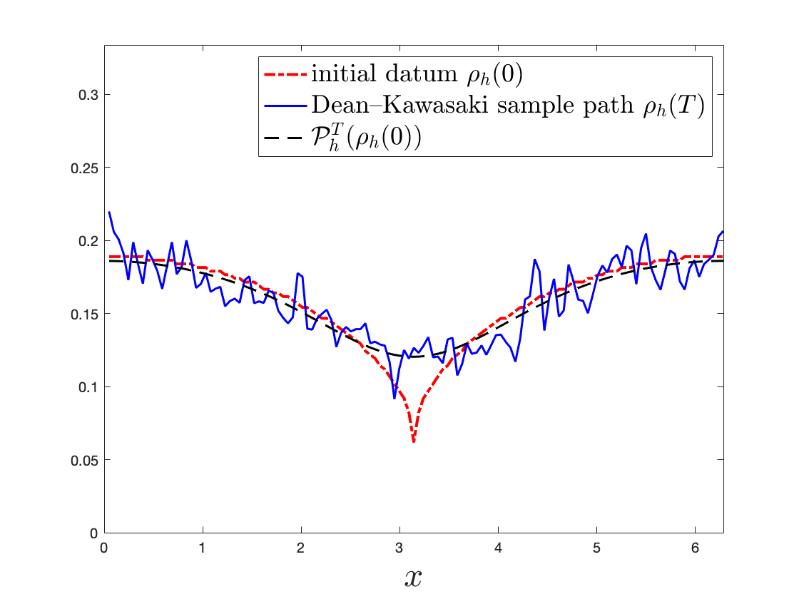
In fact, the linearised description ρ^\hat{\rho} only captures the leading-order fluctuation correction to the mean-field limit correctly and hence carries a relative error of order N−1/2N^{-1/2} with respect to the fluctuation scaling. We provide numerical evidence of such difference between the two models, and we also numerically verify convergence rates for suitable discretisations of the Dean–Kawasaki model (1).

1.1. Related Literature

The theory of fluctuating hydrodynamics describes fluctuations in interacting particle systems in the regime of large particle numbers using suitable SPDEs; see e. g. [37]. In its form (1), the Dean–Kawasaki equation describes non-interacting particles, with similar equations being available for weakly interacting particles undergoing overdamped Langevin dynamics. In the recent contribution [12], the authors also address quantitative fluctuation bounds in the non-interacting particle case, but by means of a suitable approximated SPDE model rather than a numerical scheme. While their setting grants several well-posedness results (non-negativity of the solution, comparison principles, entropy estimates) and allows to consider initial particle profiles which are more general than those treated here, their relative fluctuation error is however limited to N−1/(d/2+1)logNN^{-1/(d/2+1)}\log N, while the rate of fluctuations in (3) is – in suitable metrics – arbitrarily high.

For a more general particle setting, the SPDE of fluctuating hydrodynamics for the zero range process given by

(6) ∂tρ=Δ⁡(Φ⁡(ρ))+∇⋅(Φ⁡(ρ)​𝝃)\displaystyle\partial_{t}\rho=\Delta(\Phi(\rho))+\nabla\cdot\left(\sqrt{\Phi(\rho)}\hskip 0.60004pt\boldsymbol{\xi}\right)

has been addressed in [11], and linked it to the large deviation principle for such process in a suitable thermodynamic setting. A corresponding well-posedness result for truncated (low spatial frequency) noise and regularised nonlinearity has been obtained in [18], see also [19]. In [20], the construction of random dynamical systems for conservative SPDE is discussed, together with well-posedness theory of invariant measures and mixing of the related Markov process. In [17], a large deviation principle for regularised variants of (6) is shown; in a suitable limit, the rate functional of such large deviations principle and the corresponding one of the interacting particle system are shown to approach each other.

The paper [10], written independently of – and simultaneously to – the present manuscript, gives a rigorous justification of the fluctuating hydrodynamics SPDE associated with the symmetric simple exclusion process

∂tρ=Δ​ρ−∇⋅(ρ⁡(1−ρ)​𝝃).\displaystyle\partial_{t}\rho=\Delta\rho-\nabla\cdot\left(\sqrt{\rho(1-\rho)}\hskip 0.60004pt\boldsymbol{\xi}\right).

While in contrast to our work the authors in [10] only consider the continuum SPDE, they regularise it by truncating the noise for small spatial wavelengths. In a certain sense, this introduces a regularisation in the same spirit as our numerical approach; however, their truncation criterion is somewhat more restrictive than our condition h≫N−1/dh\gg N^{-1/d}. While they face a more challenging problem with the more complex noise intensity factor ρ⁡(1−ρ)\sqrt{\rho(1-\rho)} (whose square is not a linear function of the density ρ\rho) and also prove convergence results for the rate functions for large deviation principles, they only establish a leading-order description of fluctuations in the low deviations regime. In other words, in contrast to our present work, they do not show superiority of fluctuating hydrodynamics to a linearised approach on fluctuations for the “bulk” of the probability distribution.

For recent numerical approaches to fluctuating hydrodynamics, we refer the reader e. g. to [36, 9, 14, 3, 2, 24, 13, 33, 1] (in particular, [2] contains the extension of the current work to the case of weakly interacting particles). Note that the small prefactor of the noise term in the Dean–Kawasaki equation (1) enables the use of certain higher-order timestepping schemes [22], a fact that we also use in our numerical simulations.

Concerning further mathematical results on Dean–Kawasaki models, the link between fluctuating hydrodynamics and Wasserstein geometry has long been understood, and extensively studied in several works, see for instance [25, 38, 28, 31, 32, 30, 8].

Dean–Kawasaki type models including the effects of inertia have been derived and analysed by the first author, Shardlow, and Zimmer [4, 5, 6].

The fluctuation-dissipation relation – implicitly contained for instance in the Dean–Kawasaki equation – may be used to recover macroscopic diffusion properties from fluctuations in finite particle number simulations, see for instance [16, 33]. Outside of the realm of physics, the concept of fluctuating hydrodynamics has also been applied to systems of interacting agents, see e. g. [24, 13, 27].

Finally, conservative stochastic PDEs have recently been shown to give optimal convergence rates in the mean-field limit approximation of stochastic interacting particle systems, such as those encountered in the stochastic gradient descent methods for overparametrised, shallow neural networks [21].

Remark 1.

Given the nature of the metric dw​e​a​k,2​j−1d_{weak,2j-1} in (3), it is natural to ask whether or not the high-order fluctuation error of (3) could be formally derived from suitable a priori estimates of negative Sobolev type for the continuous Dean–Kawasaki model (1). An a purely formal level, testing the mild formulation of (1)

(7) ρ(𝒙,t)=G(t,⋅)∗ρ(⋅,0)(𝒙)+∫0t∫𝕋dG(t−s,𝒙−𝒚)∇⋅[ρ⁡(𝒚,s)ξ(𝒚,s)ds]d𝒚\displaystyle\rho(\boldsymbol{x},t)=G(t,\cdot)\ast\rho(\cdot,0)(\boldsymbol{x})+\int_{0}^{t}{\int_{\mathbb{T}^{d}}G(t-s,\boldsymbol{x}-\boldsymbol{y})\nabla\cdot\left[\sqrt{\rho(\boldsymbol{y},s)}\xi(\boldsymbol{y},s)ds\right]d\boldsymbol{y}}

– where GG is the heat semigroup kernel – with trigonometric functions, and performing elementary computations, one arrives at the a priori estimate

(8) 𝔼⁡[‖ρ(⋅,t)‖2H−j]\displaystyle\mathbb{E}\left[\mathchoice{\raisebox{0.0pt}{$\displaystyle{\vphantom{\bigm|}\mathopen{}\left\|\rho(\cdot,t)\right\|^{2}_{H^{-j}}}$}}{\left\|\rho(\cdot,t)\right\|^{2}_{H^{-j}}}{\left\|\rho(\cdot,t)\right\|^{2}_{H^{-j}}}{\left\|\rho(\cdot,t)\right\|^{2}_{H^{-j}}}\right] ≲𝔼⁡[‖ρ(⋅,0)‖2H−j]+N−1​‖ρ⁡(0)‖L1,\displaystyle\lesssim\mathbb{E}\left[\mathchoice{\raisebox{0.0pt}{$\displaystyle{\vphantom{\bigm|}\mathopen{}\left\|\rho(\cdot,0)\right\|^{2}_{H^{-j}}}$}}{\left\|\rho(\cdot,0)\right\|^{2}_{H^{-j}}}{\left\|\rho(\cdot,0)\right\|^{2}_{H^{-j}}}{\left\|\rho(\cdot,0)\right\|^{2}_{H^{-j}}}\right]+N^{-1}\|\rho(0)\|_{L^{1}},

which is valid in the regime j>d/2j>d/2.

Despite its formal validity – which, however, relies on the non-trivial negativity requirement for the density ρ\rho – the inequality (8) does not give any information beyond the leading order N−1N^{-1}, and therefore is too weak an estimate to justify the high-order fluctuation error bound in (3).

2. Main results and summary

The methodology of this paper can be applied to several standard numerical discretisations of the Dean–Kawasaki model (1), including finite difference and finite element schemes. In the interest of brevity, we only focus on a finite difference discretisation: The corresponding results in the finite element case are given in Appendix B. Specifically, on the periodic domain 𝕋d:=[−π,π)d\mathbb{T}^{d}:=[-\pi,\pi)^{d}, we denote the uniform square grid with spacing hh by Gh,dG_{h,d}, the discrete inner product of L2​(Gh,d)L^{2}(G_{h,d}) by (⋅,⋅)h(\cdot,\cdot)_{h}, the interpolating operator on Gh,dG_{h,d} by ℐh\mathcal{I}_{h}, and define the distance d−j​[𝑿,𝒀]d_{-j}[\boldsymbol{X},\boldsymbol{Y}] between two ℝM\mathbb{R}^{M}-valued random variables as

(9) d−j[𝑿,𝒀]:=supψ:max1≤j~≤j⁡‖Dj~​ψ‖L∞≤1\displaystyle d_{-j}[\boldsymbol{X},\boldsymbol{Y}]:=\sup_{\psi\colon\max_{1\leq\tilde{j}\leq j}\|D^{\tilde{j}}\psi\|_{L^{\infty}}\leq 1} |𝔼⁡[ψ(𝑿−𝔼[𝑿])]−𝔼⁡[ψ(𝒀−𝔼[𝒀])]|.\displaystyle\left|\mathbb{E}\left[\mathchoice{\raisebox{0.0pt}{$\displaystyle{\vphantom{\bigm|}\mathopen{}\psi\left(\boldsymbol{X}-\mathbb{E}[\boldsymbol{X}]\right)}$}}{\psi\left(\boldsymbol{X}-\mathbb{E}[\boldsymbol{X}]\right)}{\psi\left(\boldsymbol{X}-\mathbb{E}[\boldsymbol{X}]\right)}{\psi\left(\boldsymbol{X}-\mathbb{E}[\boldsymbol{X}]\right)}\right]-\mathbb{E}\left[\mathchoice{\raisebox{0.0pt}{$\displaystyle{\vphantom{\bigm|}\mathopen{}\psi\left(\boldsymbol{Y}-\mathbb{E}[\boldsymbol{Y}]\right)}$}}{\psi\left(\boldsymbol{Y}-\mathbb{E}[\boldsymbol{Y}]\right)}{\psi\left(\boldsymbol{Y}-\mathbb{E}[\boldsymbol{Y}]\right)}{\psi\left(\boldsymbol{Y}-\mathbb{E}[\boldsymbol{Y}]\right)}\right]\right|.

Our first main result reads as follows.

Theorem 2 (Accuracy of description of fluctuations by the finite-difference discretised Dean–Kawasaki model of order p+1∈ℕp+1\in\mathbb{N}).

Assume the validity of Assumption FD1 (discretised differential operators), Assumption FD2 (Brownian particle system), Assumption FD3 (scaling assumptions), and Assumption FD4 (discretised mean-field limit), all given below. In particular, assume that the mean-field limit ρ¯h\overline{\rho}_{h} in (21) satisfies ρm​i​n≤ρ¯h≤ρm​a​x\rho_{min}\leq\overline{\rho}_{h}\leq\rho_{max} for some positive ρm​i​n,ρm​a​x\rho_{min},\rho_{max} on [0,T][0,T]. Let ρh\rho_{h} be the solution of the discretised Dean–Kawasaki model given in Definition FD-DK on [0,T][0,T]. Set

Θ:={0,if the discretisation (16) admits a maximum principle,d/2+1,otherwise.\displaystyle\Theta:=\left\{\begin{array}[]{rl}\displaystyle 0,&\mbox{if the discretisation \eqref{eq:29} admits a maximum principle,}\\ \displaystyle d/2+1,&\mbox{otherwise.}\end{array}\right.

Then, for any j∈ℕj\in\mathbb{N}, the discrete Dean–Kawasaki model FD-DK captures the fluctuations of the empirical measure μN\mu^{N} in the sense that, for any 𝐓=(T1,…,TM)∈[0,T]M\boldsymbol{T}=(T_{1},\ldots,T_{M})\in[0,T]^{M} with 0≤T1≤⋯≤TM0\leq T_{1}\leq\dots\leq T_{M}, the inequality

d−(2​j−1)​[N1/2​((ρh​(T1),ℐh​φ1)h(ρh​(TM),ℐh​φM)h),N1/2​(⟨μT1N,φ1⟩⟨μTMN,φM⟩)]\displaystyle d_{-(2j-1)}\left[N^{1/2}\begin{pmatrix}(\rho_{h}(T_{1}),\mathcal{I}_{h}\varphi_{1})_{h}\\ \vdots\\ (\rho_{h}(T_{M}),\mathcal{I}_{h}\varphi_{M})_{h}\end{pmatrix},\penalty\ N^{1/2}\begin{pmatrix}\langle\mu^{N}_{T_{1}},\varphi_{1}\rangle\\ \vdots\\ \langle\mu^{N}_{T_{M}},\varphi_{M}\rangle\end{pmatrix}\right]
≤C⁡(M,p,j,‖𝝋‖Wp+Θ+j+1,∞,ρm​i​n,ρm​a​x,𝑻)​𝔼​[supt∈[0,T]∥ρh−(t)∥h2]1/2\displaystyle\penalty\ \penalty\ \penalty\ \penalty\ \penalty\ \penalty\ \penalty\ \penalty\ \penalty\ \penalty\ \penalty\ \penalty\ \penalty\ \penalty\ \penalty\ \penalty\ \penalty\ \penalty\ \penalty\ \leq C(M,p,j,\|\boldsymbol{\varphi}\|_{W^{p+\Theta+j+1,\infty}},\rho_{min},\rho_{max},\boldsymbol{T}){\mathbb{E}\left[\mathchoice{\raisebox{0.0pt}{$\displaystyle{\vphantom{\bigm|}\mathopen{}\sup_{t\in[0,T]}\|\rho_{h}^{-}(t)\|_{h}^{2}}$}}{\sup_{t\in[0,T]}\|\rho_{h}^{-}(t)\|_{h}^{2}}{\sup_{t\in[0,T]}\|\rho_{h}^{-}(t)\|_{h}^{2}}{\sup_{t\in[0,T]}\|\rho_{h}^{-}(t)\|_{h}^{2}}\right]^{1/2}}
+C⁡(M,p,j,‖𝝋‖Wp+Θ+j+1,∞,ρm​i​n,ρm​a​x,𝑻)​hp+1\displaystyle\penalty\ \penalty\ \penalty\ \penalty\ \penalty\ \penalty\ \penalty\ \penalty\ \penalty\ \penalty\ \penalty\ \penalty\ \penalty\ \penalty\ \penalty\ \penalty\ \penalty\ \penalty\ \penalty\ \penalty\ \penalty\ \penalty\ +C(M,p,j,\|\boldsymbol{\varphi}\|_{W^{p+\Theta+j+1,\infty}},\rho_{min},\rho_{max},\boldsymbol{T})h^{p+1}
+C(M,p,j,∥𝝋∥Wp+Θ+j+1,∞,ρm​i​n,ρm​a​x,𝑻)N−j/2\displaystyle\penalty\ \penalty\ \penalty\ \penalty\ \penalty\ \penalty\ \penalty\ \penalty\ \penalty\ \penalty\ \penalty\ \penalty\ \penalty\ \penalty\ \penalty\ \penalty\ \penalty\ \penalty\ \penalty\ \penalty\ \penalty\ \penalty\ +C(M,p,j,\|\boldsymbol{\varphi}\|_{W^{p+\Theta+j+1,\infty}},\rho_{min},\rho_{max},\boldsymbol{T})N^{-j/2}
=:Errn​e​g+Errn​u​m+Errf​l​u​c​t,r​e​l\displaystyle\penalty\ \penalty\ \penalty\ \penalty\ \penalty\ \penalty\ \penalty\ \penalty\ \penalty\ \penalty\ \penalty\ \penalty\ \penalty\ \penalty\ \penalty\ \penalty\ \penalty\ \penalty\ \penalty\ =:\mathrm{Err}_{neg}+\mathrm{Err}_{num}+\mathrm{Err}_{fluct,rel}

holds for any 𝛗=(φ1,…,φM)∈[Wp+Θ+j+1,∞​(𝕋d)]M\boldsymbol{\varphi}=(\varphi_{1},\dots,\varphi_{M})\in[W^{p+\Theta+j+1,\infty}(\mathbb{T}^{d})]^{M} such that ∥φm∥L2=1,∀m=1,…,M\|\varphi_{m}\|_{L^{2}}=1,\forall m=1,\dots,M and ∫𝕋dφk​φl​d​𝐱=0\int_{\mathbb{T}^{d}}{\varphi_{k}\varphi_{l}\emph{\mbox{d}}\boldsymbol{x}}=0 whenever Tk=TlT_{k}=T_{l}. Finally, we have the a posteriori bound

𝔼​[supt∈[0,T]∥ρh−(t)∥h2]1/2≤C​ℰ​(N,h),{\mathbb{E}\left[\mathchoice{\raisebox{0.0pt}{$\displaystyle{\vphantom{\bigm|}\mathopen{}\sup_{t\in[0,T]}\|\rho_{h}^{-}(t)\|_{h}^{2}}$}}{\sup_{t\in[0,T]}\|\rho_{h}^{-}(t)\|_{h}^{2}}{\sup_{t\in[0,T]}\|\rho_{h}^{-}(t)\|_{h}^{2}}{\sup_{t\in[0,T]}\|\rho_{h}^{-}(t)\|_{h}^{2}}\right]^{1/2}}\leq C\mathcal{E}\!\left(N,h\right),

where we have set

(12) ℰ⁡(N,h):=C⁡(d,ρm​i​n,ρm​a​x)​{exp⁡(−ρm​i​n​N1/2​hd/2C​ρm​a​x1/2)+exp⁡(−c​h−1)}.\displaystyle\mathcal{E}\!\left(N,h\right):=C(d,\rho_{min},\rho_{max})\left\{\exp\bigg(-\frac{\rho_{min}N^{1/2}h^{d/2}}{C\rho_{max}^{1/2}}\bigg)+\exp\big(-ch^{-1}\big)\right\}.

We make some observations in order to better illustrate the meaning of Theorem 2:

  • •

    The quantities (ρh​(Tm),ℐh​φm)h(\rho_{h}(T_{m}),\mathcal{I}_{h}\varphi_{m})_{h}, and ⟨μTmN,φm⟩\langle\mu_{T_{m}}^{N},\varphi_{m}\rangle are rescaled with the factor N1/2N^{1/2}, as the natural order of density fluctuations is N−1/2N^{-1/2}. In other words, our main error estimate basically provides an estimate for the relative error in the fluctuations.

  • •

    The distances d−j​[𝑿,𝒀]d_{-j}[\boldsymbol{X},\boldsymbol{Y}] correspond to negative Sobolev norm differences of the probability measures on ℝM\mathbb{R}^{M} given by the laws of 𝑿\boldsymbol{X} and 𝒀\boldsymbol{Y}. In particular, it holds d−1​[𝑿,𝒀]=𝒲1​[𝑿−𝔼⁡[𝑿],𝒀−𝔼⁡[𝒀]]d_{-1}[\boldsymbol{X},\boldsymbol{Y}]=\mathcal{W}_{1}[\boldsymbol{X}-\mathbb{E}[\boldsymbol{X}],\boldsymbol{Y}-\mathbb{E}[\boldsymbol{Y}]], where 𝒲1\mathcal{W}_{1} is the 11-Wasserstein distance.

  • •

    The above estimates contain three types of error terms. The term Errn​e​g\mathrm{Err}_{neg} quantifies the a priori lack of knowledge concerning non-negativity of the solution ρh\rho_{h}; the term Errn​u​m\mathrm{Err}_{num} encodes the numerical precision of the scheme; finally, the term Errf​l​u​c​t,r​e​l\mathrm{Err}_{fluct,rel} bounds the relative error in the fluctuations.

  • •

    The order of differentiation required for the functions 𝝋\boldsymbol{\varphi} should be thought of as the sum of p+2+Θp+2+\Theta (accounts for the requirements of the spatial discretisation, discussed below) and j−1j-1 (necessary due to an induction argument over jj).

If one is only interested in moment bounds (i.e., in a polynomial ψ\psi) then the following estimate with no relative error in the fluctuations can be produced.

Theorem 3 (Estimates on the error for stochastic moments).

In the same setting of Theorem 2, fix times 𝐓=(T1,…,TM)∈[0,T]M\boldsymbol{T}=(T_{1},\dots,T_{M})\in[0,T]^{M}, a vector 𝐣=(j1,…,jM)\boldsymbol{j}=(j_{1},\dots,j_{M}) with j:=|𝐣|1=∑m=1M|jm|j:=|\boldsymbol{j}|_{1}=\sum_{m=1}^{M}{|j_{m}|}, and a vector 𝛗=(φ1,…,φM)∈[Wp+j+1+Θ,∞]M\boldsymbol{\varphi}=(\varphi_{1},\dots,\varphi_{M})\in[W^{p+j+1+\Theta,\infty}]^{M}.

Then the difference of moments between ρh\rho_{h} and the empirical density μN\mu^{N} (2) reads

|𝔼[∏m=1M[N1/2(ρh(Tm)−𝔼[ρh(Tm)],ℐhφm)h]jm]\displaystyle\quad\left|\mathbb{E}\left[\mathchoice{\raisebox{0.0pt}{$\displaystyle{\vphantom{\bigm|}\mathopen{}\prod_{m=1}^{M}{\left[N^{1/2}(\rho_{h}(T_{m})-\mathbb{E}\left[\mathchoice{\raisebox{0.0pt}{$\displaystyle{\vphantom{\bigm|}\mathopen{}\rho_{h}(T_{m})}$}}{\rho_{h}(T_{m})}{\rho_{h}(T_{m})}{\rho_{h}(T_{m})}\right],\mathcal{I}_{h}\varphi_{m})_{h}\right]^{j_{m}}}}$}}{\prod_{m=1}^{M}{\left[N^{1/2}(\rho_{h}(T_{m})-\mathbb{E}\left[\mathchoice{\raisebox{0.0pt}{$\displaystyle{\vphantom{\bigm|}\mathopen{}\rho_{h}(T_{m})}$}}{\rho_{h}(T_{m})}{\rho_{h}(T_{m})}{\rho_{h}(T_{m})}\right],\mathcal{I}_{h}\varphi_{m})_{h}\right]^{j_{m}}}}{\prod_{m=1}^{M}{\left[N^{1/2}(\rho_{h}(T_{m})-\mathbb{E}\left[\mathchoice{\raisebox{0.0pt}{$\displaystyle{\vphantom{\bigm|}\mathopen{}\rho_{h}(T_{m})}$}}{\rho_{h}(T_{m})}{\rho_{h}(T_{m})}{\rho_{h}(T_{m})}\right],\mathcal{I}_{h}\varphi_{m})_{h}\right]^{j_{m}}}}{\prod_{m=1}^{M}{\left[N^{1/2}(\rho_{h}(T_{m})-\mathbb{E}\left[\mathchoice{\raisebox{0.0pt}{$\displaystyle{\vphantom{\bigm|}\mathopen{}\rho_{h}(T_{m})}$}}{\rho_{h}(T_{m})}{\rho_{h}(T_{m})}{\rho_{h}(T_{m})}\right],\mathcal{I}_{h}\varphi_{m})_{h}\right]^{j_{m}}}}\right]\right.
−𝔼[∏m=1M[N1/2⟨μNTm−𝔼[μNTm],φm⟩]jm]|\displaystyle\quad\quad\quad\left.-\mathbb{E}\left[\mathchoice{\raisebox{0.0pt}{$\displaystyle{\vphantom{\bigm|}\mathopen{}\prod_{m=1}^{M}{\left[N^{1/2}\langle\mu^{N}_{T_{m}}-\mathbb{E}\left[\mathchoice{\raisebox{0.0pt}{$\displaystyle{\vphantom{\bigm|}\mathopen{}\mu^{N}_{T_{m}}}$}}{\mu^{N}_{T_{m}}}{\mu^{N}_{T_{m}}}{\mu^{N}_{T_{m}}}\right],\varphi_{m}\rangle\right]^{j_{m}}}}$}}{\prod_{m=1}^{M}{\left[N^{1/2}\langle\mu^{N}_{T_{m}}-\mathbb{E}\left[\mathchoice{\raisebox{0.0pt}{$\displaystyle{\vphantom{\bigm|}\mathopen{}\mu^{N}_{T_{m}}}$}}{\mu^{N}_{T_{m}}}{\mu^{N}_{T_{m}}}{\mu^{N}_{T_{m}}}\right],\varphi_{m}\rangle\right]^{j_{m}}}}{\prod_{m=1}^{M}{\left[N^{1/2}\langle\mu^{N}_{T_{m}}-\mathbb{E}\left[\mathchoice{\raisebox{0.0pt}{$\displaystyle{\vphantom{\bigm|}\mathopen{}\mu^{N}_{T_{m}}}$}}{\mu^{N}_{T_{m}}}{\mu^{N}_{T_{m}}}{\mu^{N}_{T_{m}}}\right],\varphi_{m}\rangle\right]^{j_{m}}}}{\prod_{m=1}^{M}{\left[N^{1/2}\langle\mu^{N}_{T_{m}}-\mathbb{E}\left[\mathchoice{\raisebox{0.0pt}{$\displaystyle{\vphantom{\bigm|}\mathopen{}\mu^{N}_{T_{m}}}$}}{\mu^{N}_{T_{m}}}{\mu^{N}_{T_{m}}}{\mu^{N}_{T_{m}}}\right],\varphi_{m}\rangle\right]^{j_{m}}}}\right]\right|
≤{C⁡(d,ρm​a​x,ρm​i​n)}j/2​[∏m=1MTmjm/2]​jC1​j+C2​[∏m=1M‖φm‖Wj−1+Θ,∞jm]​𝔼​[supt∈[0,T]∥ρh−(t)∥h2]1/2\displaystyle\quad\leq\left\{C(d,\rho_{max},\rho_{min})\right\}^{j/2}\left[\prod_{m=1}^{M}{T^{j_{m}/2}_{m}}\right]j^{C_{1}j+C_{2}}\left[\prod_{m=1}^{M}{\|\varphi_{m}\|_{W^{j-1+\Theta,\infty}}^{j_{m}}}\right]{\mathbb{E}\left[\mathchoice{\raisebox{0.0pt}{$\displaystyle{\vphantom{\bigm|}\mathopen{}\sup_{t\in[0,T]}\|\rho_{h}^{-}(t)\|_{h}^{2}}$}}{\sup_{t\in[0,T]}\|\rho_{h}^{-}(t)\|_{h}^{2}}{\sup_{t\in[0,T]}\|\rho_{h}^{-}(t)\|_{h}^{2}}{\sup_{t\in[0,T]}\|\rho_{h}^{-}(t)\|_{h}^{2}}\right]^{1/2}}
+hp+1​{C⁡(d,ρm​a​x,ρm​i​n)}j/2​[∏m=1M[Tm∨Tm]jm/2]​jC3​j+C4​[∏m=1M‖φm‖Wp+j+1+Θ,∞jm]\displaystyle\quad\quad+h^{p+1}\left\{C(d,\rho_{max},\rho_{min})\right\}^{j/2}\left[\prod_{m=1}^{M}{\left[T_{m}\vee\sqrt{T}_{m}\right]^{j_{m}/2}}\right]j^{C_{3}j+C_{4}}\left[\prod_{m=1}^{M}{\|\varphi_{m}\|_{W^{p+j+1+\Theta,\infty}}^{j_{m}}}\right]
(13) =:Errn​e​g+Errn​u​m,\displaystyle\quad=:\mathrm{Err}_{neg}+\mathrm{Err}_{num},

with constants C,C1,…,C4>0C,C_{1},\dots,C_{4}>0 independent of jj, hh, NN, TT, and where we have the bound

𝔼​[supt∈[0,T]∥ρh−(t)∥h2]1/2≤C​ℰ​(N,h),{\mathbb{E}\left[\mathchoice{\raisebox{0.0pt}{$\displaystyle{\vphantom{\bigm|}\mathopen{}\sup_{t\in[0,T]}\|\rho_{h}^{-}(t)\|_{h}^{2}}$}}{\sup_{t\in[0,T]}\|\rho_{h}^{-}(t)\|_{h}^{2}}{\sup_{t\in[0,T]}\|\rho_{h}^{-}(t)\|_{h}^{2}}{\sup_{t\in[0,T]}\|\rho_{h}^{-}(t)\|_{h}^{2}}\right]^{1/2}}\leq C\mathcal{E}\!\left(N,h\right),

where ℰ⁡(N,h)\mathcal{E}\!\left(N,h\right) has been defined in (12).

2.1. Structure of the paper

Section 3 lays out the finite difference discretisation of the Dean–Kawasaki model. Subsection 3.1 (respectively, Subsection 3.2) lays out the necessary notation (respectively, the relevant assumptions and definitions) related to the model. Subsection 3.3 – which has an informal flavour – brings forward some of the main ideas used in the paper. This section lays the ground for Subsection 3.4 (respectively, Subsection 3.6), which contains preparatory results for the proofs of Theorem 2 (respectively, Theorem 3). The proof of Theorem 2 (respectively, Theorem 3) is finalised in Subsection 3.5 (respectively, Subsection 3.7). Technical details are deferred to Subsection 3.8 (bounds for all moments of ρh\rho_{h}, and exponentially decaying bound for the negative part ρh−\rho^{-}_{h}), and Appendix A (deterministic finite difference arguments and relevant Itô calculus). The statements of results for finite element schemes are given in Appendix B. Finally, Section 4 contains numerical simulations associated with Theorem 2, using a first-order finite difference discretisation (i.e., p=1p=1) in the one-dimensional case d=1d=1.

3. Analysis for finite difference discretisations

3.1. Notation

Domain and function spaces. Let ℕ∋d≤3\mathbb{N}\ni d\leq 3, and let 𝕋d:=[−π,π)d\mathbb{T}^{d}:=[-\pi,\pi)^{d}. Let h:=2​π/Lh:=2\pi/L, for some L∈2​ℕL\in 2\mathbb{N}, be the discretisation parameter of the periodic square grid

Gh,d:=h​ℤd∩𝕋d={−π,−π+h,…,π−h}d.G_{h,d}:=h\mathbb{Z}^{d}\cap\mathbb{T}^{d}=\{-\pi,-\pi+h,\dots,\pi-h\}^{d}.

We always work with periodic functions (defined either on 𝕋d\mathbb{T}^{d} or Gh,dG_{h,d}). From now on, this fact will be implicitly assumed and no longer stated. In particular, we abbreviate Cβ=Cβ​(𝕋d)C^{\beta}=C^{\beta}(\mathbb{T}^{d}) and Wr,p=Wr,p​(𝕋d)W^{r,p}=W^{r,p}(\mathbb{T}^{d}). We use bold characters to denote vector fields.

For m∈ℕm\in\mathbb{N}, let [L2​(Gh,d)]m[L^{2}(G_{h,d})]^{m} be the space of ℝm\mathbb{R}^{m}-valued functions defined on Gh,dG_{h,d}. Such space is endowed with the inner product

(𝒖h,𝒗h)h:=∑𝒙∈Gh,dhd​𝒖h​(𝒙)⋅𝒗h​(𝒙),𝒖h,𝒗h∈[L2​(Gh,d)]m,(\boldsymbol{u}_{h},\boldsymbol{v}_{h})_{h}:=\sum_{\boldsymbol{x}\in G_{h,d}}{h^{d}\boldsymbol{u}_{h}(\boldsymbol{x})\cdot\boldsymbol{v}_{h}(\boldsymbol{x})},\qquad\boldsymbol{u}_{h},\boldsymbol{v}_{h}\in[L^{2}(G_{h,d})]^{m},

and admits an orthonormal basis {𝒆𝒙,ℓm}(𝒙,ℓ)∈(Gh,d,{1,…,m})\{\boldsymbol{e}^{m}_{\boldsymbol{x},\ell}\}_{(\boldsymbol{x},\ell)\in(G_{h,d},\{1,\dots,m\})}, whose elements are defined as

𝒆𝒙,ℓm(𝒚)=h−d/2δ𝒙,𝒚𝒇ℓ,\displaystyle\boldsymbol{e}^{m}_{\boldsymbol{x},\ell}(\boldsymbol{y})=h^{-d/2}\delta_{\boldsymbol{x},\boldsymbol{y}}\boldsymbol{f}_{\ell},

where {𝒇ℓ}ℓ=1d\{\boldsymbol{f}_{\ell}\}_{\ell=1}^{d} is the canonical basis of ℝd\mathbb{R}^{d}. If m=1m=1, the notation is stripped down to

e𝒙(𝒚)=h−d/2δ𝒙,𝒚.{e}_{\boldsymbol{x}}(\boldsymbol{y})=h^{-d/2}\delta_{\boldsymbol{x},\boldsymbol{y}}.

Interpolator operator. For ϕ∈[C0]m\boldsymbol{\phi}\in[C^{0}]^{m}, we define ℐh​ϕ∈[L2​(Gh,d)]m\mathcal{I}_{h}\boldsymbol{\phi}\in[L^{2}(G_{h,d})]^{m} as the function agreeing with ϕ\boldsymbol{\phi} on Gh,dG_{h,d}. When there is no ambiguity, we simply write ϕ\boldsymbol{\phi} instead of ℐh​ϕ\mathcal{I}_{h}\boldsymbol{\phi}.

Discrete differential operators. We use the notation ∂h,xℓ\partial_{h,x_{\ell}} to denote a finite difference operator approximating the partial derivative ∂xℓ\partial_{x_{\ell}}. We denote by ∇h:=[∂h,x1,…,∂h,xd]\nabla_{h}:=[\partial_{h,x_{1}},\dots,\partial_{h,x_{d}}] the associated finite difference gradient operator. Furthermore, for each ℓ\ell, we define the discrete second partial derivative Dh,xℓ2D^{2}_{h,x_{\ell}} as the operator for which the standard integration by parts formula

(14) (Dh,xℓ2​ρh,vh)h=−(Dh,xℓ​ρh,Dh,xℓ​vh)h\displaystyle(D^{2}_{h,x_{\ell}}\rho_{h},v_{h})_{h}=-(D_{h,x_{\ell}}\rho_{h},D_{h,x_{\ell}}v_{h})_{h}

holds, where Dh,xℓD_{h,x_{\ell}} is some (possibly different) finite difference operator approximating the partial derivative ∂xℓ\partial_{x_{\ell}}. We abbreviate ∇D,h:=[Dh,x1,…,Dh,xd]\nabla_{D,h}:=[D_{h,x_{1}},\dots,D_{h,x_{d}}]. As a result of (14), the discrete operators Dh,xℓ2D^{2}_{h,x_{\ell}} are symmetric (in the sense of finite difference operators). We abbreviate

Δh:=∑ℓ=1dDh,xℓ2\displaystyle\Delta_{h}:=\sum_{\ell=1}^{d}{D^{2}_{h,x_{\ell}}}

to indicate the discrete Laplace operator. Specific details on ∇h\nabla_{h} and Δh\Delta_{h} will be provided in the following subsection.

Remark 4.

The operators ∇h\nabla_{h} and ∇D,h\nabla_{D,h} (both providing an approximation of the continuous gradient ∇\nabla) may be different, and have different uses in our discretised Dean–Kawasaki model (Definition FD-DK below). The operator ∇h\nabla_{h} is deployed in the noise, while the operator ∇D,h\nabla_{D,h} in the integration by parts formula (14).

For reasons which will become clear in Subsection 3.3 (see Block 3 therein), we set the notation for suitable continuous and discrete backwards heat flows. Specifically, for a sufficiently regular function φ\varphi and a final time TT, we denote by ϕt\phi^{t} the solution the continuous backwards heat equation

(15) ∂tϕt=−12​Δ​ϕton ​𝕋d×(0,T),\displaystyle\partial_{t}\phi^{t}=-\frac{1}{2}\Delta\phi^{t}\quad\mbox{on }\mathbb{T}^{d}\times(0,T),

with final datum ϕT=φ\phi^{T}=\varphi. Analogously, we denote by ϕht\phi_{h}^{t} the solution to the discrete backwards heat equation

(16) ∂tϕht=−12​Δh​ϕhton ​Gh,d×(0,T),\displaystyle\partial_{t}\phi_{h}^{t}=-\frac{1}{2}\Delta_{h}\phi_{h}^{t}\quad\mbox{on }G_{h,d}\times(0,T),

with final datum ϕhT=ℐh​φ\phi_{h}^{T}=\mathcal{I}_{h}\varphi. In the following, we also use the alternative notation 𝒫z​(φ):=ϕT−z\mathcal{P}^{z}(\varphi):=\phi^{T-z} (respectively, 𝒫hz​(ℐh​φ):=ϕhT−z\mathcal{P}_{h}^{z}(\mathcal{I}_{h}\varphi):=\phi_{h}^{T-z}), to stress that 𝒫z​(φ)\mathcal{P}^{z}(\varphi) (respectively, 𝒫hz​(ℐh​φ)\mathcal{P}_{h}^{z}(\mathcal{I}_{h}\varphi)) is the result of evolving a backwards heat equation (respectively, a discrete backwards heat equation) starting from φ\varphi (respectively, from ℐh​φ\mathcal{I}_{h}\varphi) for a timespan zz.

For y∈ℝy\in\mathbb{R}, we define y+:=max⁡{y;0}y^{+}:=\max\{y;0\} and y−:=−min⁡{y;0}y^{-}:=-\min\{y;0\}. In addition, as usual, we use the letter CC to denote a generic constant, whose value may change from line to line in the computations.

3.2. Assumptions and discretised Dean–Kawasaki model

Assumption FD1 (Discrete differential operators).

Let p∈ℕp\in\mathbb{N} be fixed. We make the following assumptions on the discrete operators ∂h,xℓ\partial_{h,x_{\ell}} and Dh,xℓ2D^{2}_{h,x_{\ell}}:

  • •

    the discrete operators ∂h,xℓ\partial_{h,x_{\ell}} and Dh,xℓ2D^{2}_{h,x_{\ell}} are finite difference operators of order p+1p+1. Explicitly, this means that

    (17) |∂h,xℓℐh​ϕ​(𝒙)−∂xℓϕ⁡(𝒙)|\displaystyle\left|\partial_{h,x_{\ell}}\mathcal{I}_{h}{\phi}(\boldsymbol{x})-\partial_{x_{\ell}}\phi(\boldsymbol{x})\right| ≤C​‖ϕ‖Cp+1​hp+1,𝒙∈Gh,d,ℓ∈{1,…,d},\displaystyle\leq C\|\phi\|_{C^{p+1}}h^{p+1},\qquad\boldsymbol{x}\in G_{h,d},\qquad\ell\in\{1,\dots,d\},
    (18) |Dh,xℓ2​ℐh​ϕ​(𝒙)−Dxℓ2​ϕ​(𝒙)|\displaystyle\left|D^{2}_{h,x_{\ell}}\mathcal{I}_{h}{\phi}(\boldsymbol{x})-D^{2}_{x_{\ell}}\phi(\boldsymbol{x})\right| ≤C​‖ϕ‖Cp+2​hp+1,𝒙∈Gh,d,ℓ∈{1,…,d},\displaystyle\leq C\|\phi\|_{C^{p+2}}h^{p+1},\qquad\boldsymbol{x}\in G_{h,d},\qquad\ell\in\{1,\dots,d\},

    for any ϕ∈Cp+2​(𝕋d)\phi\in C^{p+2}(\mathbb{T}^{d});

  • •

    The operators ∂h,xℓ\partial_{h,x_{\ell}} and Dh,xℓ2D^{2}_{h,x_{\ell}} commute.

Assumption FD2 (Brownian particle system and initial datum of Dean–Kawasaki dynamics).

Let pp be as in Assumption FD1. We assume to have N∈ℕN\in\mathbb{N} independent dd-dimensional Brownian motions {𝐰k}k=1N\{\boldsymbol{w}_{k}\}_{k=1}^{N} moving in 𝕋d\mathbb{T}^{d}. Moreover:

  • •

    the initial positions {𝒘k​(0)}k=1N\{\boldsymbol{w}_{k}(0)\}_{k=1}^{N} are deterministic;

  • •

    there exists a deterministic function ρ0,h∈L2​(Gh,d)\rho_{0,h}\in L^{2}(G_{h,d}) (which will serve as the initial datum of the discretised Dean–Kawasaki dynamics in Definition FD-DK below), satisfying the following properties:

    • –

      there exist hh-independent constants ρm​i​n\rho_{min} and ρm​a​x\rho_{max} such that

      0<ρm​i​n≤ρ0,h≤ρm​a​x;\displaystyle 0<\rho_{min}\leq\rho_{0,h}\leq\rho_{max};
    • –

      the empirical density of the initial configuration μ0N:=N−1​∑k=1Nδ𝒘k​(0)\mu^{N}_{0}:=N^{-1}\sum_{k=1}^{N}{\delta_{\boldsymbol{w}_{k}(0)}} approximates ρ0,h\rho_{0,h} with accuracy p+1p+1, in the sense that the inequality

      |⟨μ0N,η⟩−(ρ0,h,ℐh​η)h|\displaystyle\left|\langle\mu^{N}_{0},\eta\rangle-(\rho_{0,h},\mathcal{I}_{h}\eta)_{h}\right|
      (19) =|N−1​∑k=1Nη⁡(𝒘k​(0))−(ρ0,h,ℐh​η)h|≤C​hp+1​‖η‖Cp+1,\displaystyle\quad=\left|N^{-1}\sum_{k=1}^{N}{\eta(\boldsymbol{w}_{k}(0))}-(\rho_{0,h},\mathcal{I}_{h}\eta)_{h}\right|\leq Ch^{p+1}\|\eta\|_{C^{p+1}},

      holds for each function η∈Cp+1\eta\in C^{p+1}.

Assumption FD3 (Scaling of relevant parameters).

We assume the scaling

(20) h≥C(d,ρm​i​n,ρm​a​x)N−1/d|logN|2/d(1+T),\displaystyle h\geq C(d,\rho_{min},\rho_{max})N^{-1/d}|\log N|^{2/d}(1+T),

for some T>0T>0, and where ρm​i​n\rho_{min} and ρm​a​x\rho_{max} have been introduced in Assumption FD2. This scaling will be needed to produce an exponentially decaying estimate associated with ρh−\rho_{h}^{-}, see (67) below.

Assumption FD4 (Mean-field limit).

The solution to the discrete heat equation

(21) {∂tρ¯h=12​Δh​ρ¯h,ρ¯h​(0)=ρ0,h,\left\{\quad\begin{aligned} \!\!\!\!\!\partial_{t}\overline{\rho}_{h}&=\frac{1}{2}\Delta_{h}\overline{\rho}_{h},\\ \!\!\!\!\!\overline{\rho}_{h}(0)&=\rho_{0,h},\end{aligned}\right.

is such that ρm​i​n≤ρ¯h≤ρm​a​x\rho_{min}\leq\overline{\rho}_{h}\leq\rho_{max} (where ρm​i​n\rho_{min} and ρm​a​x\rho_{max} have been introduced in Assumption FD2) for all times up to TT (where TT has have been introduced in Assumption FD3).

We can now state the precise definition of our finite difference Dean–Kawasaki model.

Definition FD-DK (Finite difference Dean–Kawasaki model of order p+1p+1).

Assume the validity of Assumptions FD1–FD4. We say that the L2​(Gh,d)L^{2}(G_{h,d})-valued process ρh\rho_{h} solves a finite difference Dean–Kawasaki model of order p+1p+1 if it solves the system of stochastic differential equations

(22) {d​(ρh,e𝒙)h=12(Δhρh,e𝒙)hdt−N−1/2∑(𝒚,ℓ)∈(Gh,d,{1,…,d})(ℱρ𝒆dh,𝒚,ℓ,∇he𝒙)hdβ(𝒚,ℓ),∀e𝒙,ρh​(0)=ρ0,h,\left\{\begin{aligned} \mbox{d}\left(\rho_{h},e_{\boldsymbol{x}}\right)_{h}&=\frac{1}{2}\left(\Delta_{h}\rho_{h},e_{\boldsymbol{x}}\right)_{h}\mbox{d}t-N^{-1/2}\!\!\!\!\!\!\!\!\!\sum_{(\boldsymbol{y},\ell)\in(G_{h,d},\{1,\dots,d\})}{\!\!\!\!\left(\mathcal{F}_{\rho}\boldsymbol{e}^{d}_{h,\boldsymbol{y},\ell},\nabla_{h}e_{\boldsymbol{x}}\right)_{h}\mbox{d}\beta_{(\boldsymbol{y},\ell)}},\quad\forall e_{\boldsymbol{x}},\\ \rho_{h}(0)&=\rho_{0,h},\end{aligned}\right.

where {β(𝐲,ℓ)}(𝐲,ℓ)∈(Gh,d,{1,…,d})\{\beta_{(\boldsymbol{y},\ell)}\}_{(\boldsymbol{y},\ell)\in(G_{h,d},\{1,\dots,d\})} are standard independent Brownian motions, and where ℱρ∈L2​(Gh,d)\mathcal{F}_{\rho}\in L^{2}(G_{h,d}) is defined as

(23) ℱρ​(𝒙):=ρh+​(𝒙),∀𝒙∈Gh,d.\displaystyle\mathcal{F}_{\rho}(\boldsymbol{x}):=\sqrt{\rho_{h}^{+}(\boldsymbol{x})},\qquad\forall\boldsymbol{x}\in G_{h,d}.
Remark 5.

If (21) admits a discrete maximum principle, then Assumption FD4 is satisfied for any T>0T>0 and any non-negative datum ρ0,h\rho_{0,h}. For example, the discrete maximum principle applies for the second-order symmetrical discrete Laplace operator

(24) Δh​f​(𝒙):=−2​d​fh​(𝒙)+∑𝒚∼𝒙fh​(𝒚)h2,\displaystyle\Delta_{h}f(\boldsymbol{x}):=\frac{-2d\hskip 0.06006ptf_{h}(\boldsymbol{x})+\sum_{\boldsymbol{y}\sim\boldsymbol{x}}{f_{h}(\boldsymbol{y})}}{h^{2}},

where 𝐲∼𝐱\boldsymbol{y}\sim\boldsymbol{x} indicates that 𝐲\boldsymbol{y} and 𝐱\boldsymbol{x} are adjacent grid points.

Remark 6.

One may also omit the contribution (1+T)(1+T) in the scaling (20), at the expense of obtaining results with a worse dependency on the final time TT. We are not interested in optimising time dependencies in this work, and we simply include the term 1+T1+T in order to get cleaner final results.

3.3. Key ideas behind the proofs of the main results

The proofs of Theorems 2 and 3 are of inductive type. In order to simplify their exposition, it is useful to first list a skeleton of the main building blocks.

Block 1. Discrete Dean–Kawasaki model: cross-variation analysis. At their core, both proofs use basic Itô calculus to describe the time evolution of suitable nonlinear functionals ψ\psi of the quantities

(25) (ρh,ϕh)h,(μN,ϕ),\displaystyle(\rho_{h},\phi_{h})_{h},\qquad(\mu^{N},\phi),

and of their expected values, where ϕh\phi_{h} and ϕ\phi are suitable test functions. The quantities in (25) are linear functionals of ρh\rho_{h} and μN\mu^{N}, respectively. What is crucial, is that the cross-variation of the processes (25) are – up to a small error – also linear functionals of ρh\rho_{h} and μN\mu^{N}. The argument for μN\mu^{N} is straightforward, and we can thus defer it to the proofs themselves. As for ρh\rho_{h}, we use Definition FD-DK to write

(26) d​(ρh,ϕi,h)h\displaystyle\mbox{d}(\rho_{h},\phi_{i,h})_{h} =12(Δhρh,ϕi,h)hdt−N−1/2∑(𝒚,ℓ)∈(Gh,d,{1,…,d})(ℱρ𝒆h,𝒚,ℓd,∇hϕi,h)hdβ(𝒚,ℓ)\displaystyle=\frac{1}{2}(\Delta_{h}\rho_{h},\phi_{i,h})_{h}\mbox{d}t-N^{-1/2}\!\!\!\!\!\!\!\!\sum_{(\boldsymbol{y},\ell)\in(G_{h,d},\{1,\dots,d\})}{\!\!\!\left(\mathcal{F}_{\rho}\boldsymbol{e}^{d}_{h,\boldsymbol{y},\ell},\nabla_{h}\phi_{i,h}\right)_{h}\mbox{d}\beta_{(\boldsymbol{y},\ell)}}

for two different test functions ϕi,h\phi_{i,h}, i∈{1,2}i\in\{1,2\}. Using the Itô formula and the Parseval identity in [L2​(Gh,d)]d[L^{2}(G_{h,d})]^{d}, one finds that the cross-variation of the stochastic noise of (26) is

⟨∑(𝒚,ℓ)∈(Gh,d,{1,…,d})(ℱρ​𝒆h,𝒚,ℓd,∇hϕ1,h)h​β˙(𝒚,ℓ),∑(𝒚,ℓ)∈(Gh,d,{1,…,d})(ℱρ​𝒆h,𝒚,ℓd,∇hϕ2,h)h​β˙(𝒚,ℓ)⟩\displaystyle\left\langle\sum_{(\boldsymbol{y},\ell)\in(G_{h,d},\{1,\dots,d\})}{\!\!\!\!\!\left(\mathcal{F}_{\rho}\boldsymbol{e}^{d}_{h,\boldsymbol{y},\ell},\nabla_{h}\phi_{1,h}\right)_{h}\dot{\beta}_{(\boldsymbol{y},\ell)}},\,\sum_{(\boldsymbol{y},\ell)\in(G_{h,d},\{1,\dots,d\})}{\!\!\!\!\!\left(\mathcal{F}_{\rho}\boldsymbol{e}^{d}_{h,\boldsymbol{y},\ell},\nabla_{h}\phi_{2,h}\right)_{h}\dot{\beta}_{(\boldsymbol{y},\ell)}}\right\rangle
(27) =∑(𝒚,ℓ)∈(Gh,d,{1,…,d})(𝒆h,𝒚,ℓd,ℱρ​∇hϕ1,h)h​(𝒆h,𝒚,ℓd,ℱρ​∇hϕ2,h)h\displaystyle\quad=\sum_{(\boldsymbol{y},\ell)\in(G_{h,d},\{1,\dots,d\})}{\left(\boldsymbol{e}^{d}_{h,\boldsymbol{y},\ell},\mathcal{F}_{\rho}\nabla_{h}\phi_{1,h}\right)_{h}\left(\boldsymbol{e}^{d}_{h,\boldsymbol{y},\ell},\mathcal{F}_{\rho}\nabla_{h}\phi_{2,h}\right)_{h}}
(28) =(ℱρ2,∇hϕ1,h⋅∇hϕ2,h)h\displaystyle\quad=\left(\mathcal{F}^{2}_{\rho},\nabla_{h}\phi_{1,h}\cdot\nabla_{h}\phi_{2,h}\right)_{h}
(29) =(23)(ρh+,∇hϕ1,h⋅∇hϕ2,h)h\displaystyle\quad\stackrel{{\scriptstyle\mathclap{\eqref{e:13}}}}{{=}}\,\left(\rho^{+}_{h},\nabla_{h}\phi_{1,h}\cdot\nabla_{h}\phi_{2,h}\right)_{h}
(30) =(ρh,∇hϕ1,h⋅∇hϕ2,h)h+(ρh−,∇hϕ1,h⋅∇hϕ2,h)h.\displaystyle\quad=\left(\rho_{h},\nabla_{h}\phi_{1,h}\cdot\nabla_{h}\phi_{2,h}\right)_{h}+\left(\rho^{-}_{h},\nabla_{h}\phi_{1,h}\cdot\nabla_{h}\phi_{2,h}\right)_{h}.

The first term in (30) is indeed a linear functional of ρh\rho_{h}. The second term (which we will show to be negligible for suitable scaling regimes, see Subsection 3.8) takes into account the a priori lack of knowledge concerning the non-negativity of solutions to the discrete Dean–Kawasaki model (22). We also stress that the validity of the computations above is independent of the order of the finite difference scheme (i.e., pp).

Expression (29) crucially preserves the cross-variation structure associated with the continuous Dean–Kawasaki (1) for nonnegative densities. More precisely, formally testing (1) with a smooth test functions ϕi\phi_{i}, i∈{1,2}i\in\{1,2\}, gives

∫𝕋d∂tρ​ϕi​d​𝒙\displaystyle\int_{\mathbb{T}^{d}}{\partial_{t}\rho\,\phi_{i}}\mbox{d}\boldsymbol{x} =12∫𝕋dΔρϕid𝒙−N−1/2∫𝕋du𝝃⋅∇ϕid𝒙\displaystyle=\frac{1}{2}\int_{\mathbb{T}^{d}}{\Delta\rho\,\phi_{i}\mbox{d}\boldsymbol{x}}-N^{-1/2}\int_{\mathbb{T}^{d}}{\sqrt{u}\,\boldsymbol{\xi}\cdot\nabla\phi_{i}\mbox{d}\boldsymbol{x}}
(31) =12∫𝕋dΔρϕid𝒙−N−1/2∑𝒔∈ℤ∫𝕋dρ𝒆𝒔⋅∇ϕid𝒙β˙𝒔,\displaystyle=\frac{1}{2}\int_{\mathbb{T}^{d}}{\Delta\rho\,\phi_{i}\mbox{d}\boldsymbol{x}}-N^{-1/2}\sum_{{\boldsymbol{s}}\in\mathbb{Z}}{\int_{\mathbb{T}^{d}}{\sqrt{\rho}\,\boldsymbol{e}_{\boldsymbol{s}}\cdot\nabla\phi_{i}\mbox{d}\boldsymbol{x}\dot{\beta}_{\boldsymbol{s}}}},

where the last inequality if justified by the representation 𝝃=∑𝒔∈ℤd𝒆𝒔​β˙𝒔\boldsymbol{\xi}=\sum_{\boldsymbol{s}\in\mathbb{Z}^{d}}\boldsymbol{e}_{\boldsymbol{s}}\dot{\beta}_{\boldsymbol{s}}, where {𝒆𝒔}𝒔∈ℤd\{\boldsymbol{e}_{\boldsymbol{s}}\}_{{\boldsymbol{s}}\in\mathbb{Z}^{d}} is an orthonormal basis of [L2​(𝕋d)]d[L^{2}(\mathbb{T}^{d})]^{d} and {β𝒔}𝒔∈ℤd\{\beta_{\boldsymbol{s}}\}_{\boldsymbol{s}\in\mathbb{Z}^{d}} are independent Brownian motions. The noise cross-variation is then obtained using the Itô formula and the Parseval idendity – this time in [L2​(𝕋d)]d[L^{2}(\mathbb{T}^{d})]^{d} – to obtain

⟨∑𝒌∈ℤd∫𝕋dρ𝒆𝒌⋅∇ϕ1d𝒙β˙𝒌,∑𝒍∈ℤd∫𝕋dρ𝒆𝒍⋅∇ϕ2d𝒙β˙𝒍⟩\displaystyle\left\langle\sum_{\boldsymbol{k}\in\mathbb{Z}^{d}}{\int_{\mathbb{T}^{d}}{\sqrt{\rho}\boldsymbol{e}_{\boldsymbol{k}}\cdot\nabla\phi_{1}\mbox{d}\boldsymbol{x}\dot{\beta}_{\boldsymbol{k}}}},\sum_{{\boldsymbol{l}}\in\mathbb{Z}^{d}}{\int_{\mathbb{T}^{d}}{\sqrt{\rho}\boldsymbol{e}_{\boldsymbol{l}}\cdot\nabla\phi_{2}\mbox{d}\boldsymbol{x}\dot{\beta}_{\boldsymbol{l}}}}\right\rangle
(32) =∑𝒌∈ℤ∫𝕋dρ𝒆k⋅∇ϕ1d𝒙∫𝕋dρ𝒆k⋅∇ϕ2d𝒙=∫𝕋dρ∇ϕ1⋅∇ϕ2d𝒙,\displaystyle\quad=\sum_{{\boldsymbol{k}}\in\mathbb{Z}}{\int_{\mathbb{T}^{d}}{\sqrt{\rho}\boldsymbol{e}_{k}\cdot\nabla\phi_{1}}\mbox{d}\boldsymbol{x}}\int_{\mathbb{T}^{d}}{\sqrt{\rho}\boldsymbol{e}_{k}\cdot\nabla\phi_{2}\mbox{d}\boldsymbol{x}}=\int_{\mathbb{T}^{d}}{\rho\nabla\phi_{1}\cdot\nabla\phi_{2}\mbox{d}\boldsymbol{x}},

and thus the cross-variations (3.3) and (29) are (modulo positive part ρh+\rho_{h}^{+}) structurally identical.

Block 2. Numerical error. There are two contributions to the numerical error, namely:

  1. -

    the difference of initial data μ0N\mu^{N}_{0} and ρh​(0)\rho_{h}(0), and

  2. -

    the difference in the evolution of test functions (say, ϕ\phi and ϕh\phi_{h}),

and both are proportional to hp+1h^{p+1}. While the first contribution has the correct bound by Assumption FD2, the second contribution needs to be estimated: The main difficulty is that the interpolation of the test function arising from the cross-variation of the second quantity in (25) (i.e., ℐh​(∇ϕ1⋅∇ϕ2)\mathcal{I}_{h}(\nabla\phi_{1}\cdot\nabla\phi_{2})) does not coincide – in general – with ∇hϕ1,h⋅∇hϕ2,h\nabla_{h}\phi_{1,h}\cdot\nabla_{h}\phi_{2,h} (i.e., the cross-variation of the first quantity in (25)). We therefore need to show the bound

|ℐh​(∇ϕ1⋅∇ϕ2)−∇hϕ1,h⋅∇hϕ2,h|≲hp+1\left|\mathcal{I}_{h}(\nabla\phi_{1}\cdot\nabla\phi_{2})-\nabla_{h}\phi_{1,h}\cdot\nabla_{h}\phi_{2,h}\right|\lesssim h^{p+1}

in order not to lose hh-regularity in consecutive steps of our inductive proofs (more details in Block 5 below). The necessary tools for this task are contained in Subsection A.1.

Block 3. Deterministic dynamics of the test functions. As we are interested only in the analysis of the fluctuations for the Dean–Kawasaki model, it is convenient to choose the deterministic functions ψ\psi, ϕ\phi, ϕh\phi_{h} in such a way that as many drift terms as possible in relevant Itô differentials vanish. This is the reason behind the choice of the backwards heat equation (15) (respectively, (16)) for ϕ\phi (respectively, for ϕh\phi_{h}), which directly compensates the diffusive nature of the particle system (respectively, of the Dean–Kawasaki model). In practice, this is reflected in the useful equalities (which follow from Lemma 15)

(33) (ρh​(t),ϕht)h−(ρh​(0),ϕh0)h\displaystyle(\rho_{h}(t),\phi_{h}^{t})_{h}-(\rho_{h}(0),\phi_{h}^{0})_{h} =(ρh​(t)−𝔼⁡[ρh(t)],ϕht)h,\displaystyle=(\rho_{h}(t)-\mathbb{E}\left[\mathchoice{\raisebox{0.0pt}{$\displaystyle{\vphantom{\bigm|}\mathopen{}\rho_{h}(t)}$}}{\rho_{h}(t)}{\rho_{h}(t)}{\rho_{h}(t)}\right],\phi_{h}^{t})_{h},
(34) ⟨μtN,ϕt⟩−⟨μ0N,ϕ0⟩\displaystyle\langle\mu^{N}_{t},\phi^{t}\rangle-\langle\mu^{N}_{0},\phi^{0}\rangle =⟨μtN−𝔼⁡[μNt],ϕt⟩,\displaystyle=\langle\mu^{N}_{t}-\mathbb{E}\left[\mathchoice{\raisebox{0.0pt}{$\displaystyle{\vphantom{\bigm|}\mathopen{}\mu^{N}_{t}}$}}{\mu^{N}_{t}}{\mu^{N}_{t}}{\mu^{N}_{t}}\right],\phi^{t}\rangle,

for ϕ,ϕh\phi,\phi_{h} as in (15), (16). The discussion for ψ\psi in the case of Theorem 2 is conceptually analogous, but technically more involved, and is devolved to the proof itself. As for Theorem 3, ψ\psi is chosen to be static, therefore this discussion does not apply.

We expand these considerations in Appendix A.2.

Block 4. Stretched exponential bounds for centred moments of the particle system and the Dean–Kawasaki solution. This block associates the scaling regime of Assumption FD3 to the validity of the moment bounds

maxt∈[0,T]⁡𝔼⁡[|∏m=1M⟨μNTm−𝔼[μNTm],φm⟩jm|]\displaystyle\max_{t\in[0,T]}{\mathbb{E}\left[\mathchoice{\raisebox{0.0pt}{$\displaystyle{\vphantom{\bigm|}\mathopen{}\left|\prod_{m=1}^{M}{\langle\mu^{N}_{T_{m}}-\mathbb{E}\left[\mathchoice{\raisebox{0.0pt}{$\displaystyle{\vphantom{\bigm|}\mathopen{}\mu^{N}_{T_{m}}}$}}{\mu^{N}_{T_{m}}}{\mu^{N}_{T_{m}}}{\mu^{N}_{T_{m}}}\right],\varphi_{m}\rangle^{j_{m}}}\right|}$}}{\left|\prod_{m=1}^{M}{\langle\mu^{N}_{T_{m}}-\mathbb{E}\left[\mathchoice{\raisebox{0.0pt}{$\displaystyle{\vphantom{\bigm|}\mathopen{}\mu^{N}_{T_{m}}}$}}{\mu^{N}_{T_{m}}}{\mu^{N}_{T_{m}}}{\mu^{N}_{T_{m}}}\right],\varphi_{m}\rangle^{j_{m}}}\right|}{\left|\prod_{m=1}^{M}{\langle\mu^{N}_{T_{m}}-\mathbb{E}\left[\mathchoice{\raisebox{0.0pt}{$\displaystyle{\vphantom{\bigm|}\mathopen{}\mu^{N}_{T_{m}}}$}}{\mu^{N}_{T_{m}}}{\mu^{N}_{T_{m}}}{\mu^{N}_{T_{m}}}\right],\varphi_{m}\rangle^{j_{m}}}\right|}{\left|\prod_{m=1}^{M}{\langle\mu^{N}_{T_{m}}-\mathbb{E}\left[\mathchoice{\raisebox{0.0pt}{$\displaystyle{\vphantom{\bigm|}\mathopen{}\mu^{N}_{T_{m}}}$}}{\mu^{N}_{T_{m}}}{\mu^{N}_{T_{m}}}{\mu^{N}_{T_{m}}}\right],\varphi_{m}\rangle^{j_{m}}}\right|}\right]} ≤{N−1​T}j/2​jj​[∏m=1M‖∇φm‖∞jm]\displaystyle\leq\left\{N^{-1}T\right\}^{j/2}j^{j}\left[\prod_{m=1}^{M}{\|\nabla\varphi_{m}\|_{\infty}^{j_{m}}}\right]

and

maxt∈[0,T]⁡𝔼⁡[|∏m=1M(ρh(Tm)−𝔼[ρh(Tm)],ℐhφm)hjm|]\displaystyle\max_{t\in[0,T]}{\mathbb{E}\left[\mathchoice{\raisebox{0.0pt}{$\displaystyle{\vphantom{\bigm|}\mathopen{}\left|\prod_{m=1}^{M}{\left(\rho_{h}(T_{m})-\mathbb{E}\left[\mathchoice{\raisebox{0.0pt}{$\displaystyle{\vphantom{\bigm|}\mathopen{}\rho_{h}(T_{m})}$}}{\rho_{h}(T_{m})}{\rho_{h}(T_{m})}{\rho_{h}(T_{m})}\right],\mathcal{I}_{h}\varphi_{m}\right)_{h}^{j_{m}}}\right|}$}}{\left|\prod_{m=1}^{M}{\left(\rho_{h}(T_{m})-\mathbb{E}\left[\mathchoice{\raisebox{0.0pt}{$\displaystyle{\vphantom{\bigm|}\mathopen{}\rho_{h}(T_{m})}$}}{\rho_{h}(T_{m})}{\rho_{h}(T_{m})}{\rho_{h}(T_{m})}\right],\mathcal{I}_{h}\varphi_{m}\right)_{h}^{j_{m}}}\right|}{\left|\prod_{m=1}^{M}{\left(\rho_{h}(T_{m})-\mathbb{E}\left[\mathchoice{\raisebox{0.0pt}{$\displaystyle{\vphantom{\bigm|}\mathopen{}\rho_{h}(T_{m})}$}}{\rho_{h}(T_{m})}{\rho_{h}(T_{m})}{\rho_{h}(T_{m})}\right],\mathcal{I}_{h}\varphi_{m}\right)_{h}^{j_{m}}}\right|}{\left|\prod_{m=1}^{M}{\left(\rho_{h}(T_{m})-\mathbb{E}\left[\mathchoice{\raisebox{0.0pt}{$\displaystyle{\vphantom{\bigm|}\mathopen{}\rho_{h}(T_{m})}$}}{\rho_{h}(T_{m})}{\rho_{h}(T_{m})}{\rho_{h}(T_{m})}\right],\mathcal{I}_{h}\varphi_{m}\right)_{h}^{j_{m}}}\right|}\right]}
≤{2​N−1​T​C​(d,ρm​i​n,ρm​a​x)}j/2​j3​j​(∏m=1M‖φm‖C1+Θjm),\displaystyle\quad\leq\left\{2N^{-1}TC\left(d,\rho_{min},\rho_{max}\right)\right\}^{j/2}j^{3j}\left(\prod_{m=1}^{M}{\|\varphi_{m}\|_{C^{1+\Theta}}^{j_{m}}}\right),

where T1,…,Tm∈[0,T]T_{1},\dots,T_{m}\in[0,T], and Θ\Theta was introduced in (2). The difference in the norms of the test functions stems from a difference in underlying mathematical arguments (depending on the circumstance, we will either use the maximum principle or the Sobolev embedding Theorem). The necessary tools for this point are contained in Subsection A.2.

Block 5. Inductive argument. Block 1 essentially states that computing cross-variations of discrete Dean–Kawasaki models yields linear functionals (25), as well as negligible corrections related to the negative part ρh−\rho^{-}_{h}. Taking Block 2 also into account, this leads to the following crucial observation.

The Itô correction term in the Itô differential of smooth enough nonlinear functions ψ\psi applied to (25) and their expected values is a sum of:

  1. -

    negligible terms featuring ρh−\rho^{-}_{h} and the numerical error, and

  2. -

    yet another (possibly different) nonlinear function ψ~\tilde{\psi} applied to (25) and their expected values.

This property allows to set up both proofs using an induction argument whose inductive step is the change in nonlinear function (from ψ\psi to ψ~\tilde{\psi}): the residual terms (featuring ρh−\rho^{-}_{h} and the numerical error) are estimated at each step, and are not fed to the next step.

3.4. The key step for the accuracy estimate for fluctuations in Theorem 2

For use in the next proposition, we define the two function spaces ℒpow,rq,ℒ~pow,rq\mathcal{L}_{\text{pow,r}}^{q},{\tilde{\mathcal{L}}}_{\text{pow,r}}^{q} as

ℒpow,rq:={ψ:ℝM→ℝ:∥ψ∥ℒpow,rq:=max0≤q~≤q‖(1+|⋅|2)−r/2Dq~ψ(⋅)‖L∞<∞},\displaystyle\mathcal{L}_{\text{pow,r}}^{q}:=\left\{\psi:\mathbb{R}^{M}\rightarrow\mathbb{R}\colon\|\psi\|_{\mathcal{L}_{\text{pow,r}}^{q}}:=\max_{0\leq\tilde{q}\leq q}\left\|(1+|\cdot|^{2})^{-r/2}D^{\tilde{q}}\psi(\cdot)\right\|_{L^{\infty}}<\infty\right\},
ℒ~pow,rq:={ψ:ℝM→ℝ:∥ψ∥ℒpow,rq:=max1≤q~≤q‖(1+|⋅|2)−r/2Dq~ψ(⋅)‖L∞<∞}.\displaystyle{\tilde{\mathcal{L}}}_{\text{pow,r}}^{q}:=\left\{\psi:\mathbb{R}^{M}\rightarrow\mathbb{R}\colon\|\psi\|_{\mathcal{L}_{\text{pow,r}}^{q}}:=\max_{1\leq\tilde{q}\leq q}\left\|(1+|\cdot|^{2})^{-r/2}D^{\tilde{q}}\psi(\cdot)\right\|_{L^{\infty}}<\infty\right\}.

Furthermore, we emphasise that we use the shorthand notations

⟨μ𝑻N−𝔼⁡[μ𝑻N],ϕ⟩\displaystyle\langle\mu_{\boldsymbol{T}}^{N}-\mathbb{E}[\mu_{\boldsymbol{T}}^{N}],\boldsymbol{\phi}\rangle :=(⟨μT1N−𝔼⁡[μT1N],ϕ1⟩⟨μTMN−𝔼⁡[μTMN],ϕM⟩),\displaystyle:=\begin{pmatrix}\langle\mu_{T_{1}}^{N}-\mathbb{E}[\mu_{T_{1}}^{N}],\phi_{1}\rangle\\ \vdots\\ \langle\mu_{T_{M}}^{N}-\mathbb{E}[\mu_{T_{M}}^{N}],\phi_{M}\rangle\end{pmatrix},
((ρh​(𝑻)−𝔼⁡[ρh​(𝑻)]),ϕh)h\displaystyle\big((\rho_{h}(\boldsymbol{T})-\mathbb{E}[\rho_{h}(\boldsymbol{T})]),\boldsymbol{\phi}_{h}\big)_{h} :=(((ρh​(T1)−𝔼⁡[ρh​(T1)]),ϕ1,h)h((ρh​(TM)−𝔼⁡[ρh​(TM)]),ϕM,h)h),\displaystyle:=\begin{pmatrix}\big((\rho_{h}(T_{1})-\mathbb{E}[\rho_{h}(T_{1})]),\phi_{1,h}\big)_{h}\\ \vdots\\ \big((\rho_{h}(T_{M})-\mathbb{E}[\rho_{h}(T_{M})]),\phi_{M,h}\big)_{h}\end{pmatrix},
((ρh−𝔼⁡[ρh]),ϕh)h​(𝑻)\displaystyle\big((\rho_{h}-\mathbb{E}[\rho_{h}]),\boldsymbol{\phi}_{h}\big)_{h}(\boldsymbol{T}) :=((ρh​(𝑻)−𝔼⁡[ρh​(𝑻)]),ϕh𝑻)h,\displaystyle:=\big((\rho_{h}(\boldsymbol{T})-\mathbb{E}[\rho_{h}(\boldsymbol{T})]),\boldsymbol{\phi}_{h}^{\boldsymbol{T}}\big)_{h},
t∧𝑻\displaystyle t\wedge\boldsymbol{T} :=(t∧T1,…,t∧TM),\displaystyle:=(t\wedge T_{1},\dots,t\wedge T_{M}),

i.e., we implicitly multiply vectors in an element-wise fashion respectively evaluate vectorial functions by a vector of (time) parameters in an element-wise way.

Theorem 2 will be seen to be an easy consequence of the following crucial proposition and an inductive argument.

Proposition 7.

Let μtN\mu_{t}^{N} denote the empirical measure of NN independent Brownian particles as defined in (2).

Let ρh\rho_{h} be a solution to the Dean–Kawasaki equation discretised using finite differences on a uniform grid (22). Suppose furthermore that Assumption FD1 (details of operators Δh\Delta_{h} and ∇h\nabla_{h}), Assumption FD2 (initial condition on Brownian particle system), Assumption FD3 (scaling assumptions), and Assumption FD4 (positivity-preserving properties of mean-field limit) hold.

Let MM, p∈ℕp\in\mathbb{N}, q∈ℕq\in\mathbb{N}, and r∈ℕ0r\in\mathbb{N}_{0}. Let ψ:ℝM→ℝ\psi:\mathbb{R}^{M}\rightarrow\mathbb{R} satisfy ψ∈ℒpow,rq+2\psi\in\mathcal{L}_{\text{pow,r}}^{q+2}. Let 𝛗∈[W2+p+Θ,∞]M\boldsymbol{\varphi}\in[W^{2+p+\Theta,\infty}]^{M}. Finally, let 𝐓=(T1,…,TM)\boldsymbol{T}=(T_{1},\dots,T_{M}) such that 0<T1≤…≤TM≤T0<T_{1}\leq\ldots\leq T_{M}\leq T.

Then there exist test functions ψ~k​lt\tilde{\psi}^{t}_{kl}, ϕ~k​lt\tilde{\boldsymbol{\phi}}^{t}_{kl}, ψ0\psi^{0}, and ϕ0\boldsymbol{\phi}^{0} as well as 𝐓~k​l∈ℝM+1\boldsymbol{\tilde{T}}_{kl}\in\mathbb{R}^{M+1} such that

(35a) 𝔼⁡[ψ⁡(N1/2​⟨μ𝑻N−𝔼⁡[μ𝑻N],𝝋⟩)]\displaystyle\mathbb{E}\Bigg[\psi\bigg(N^{1/2}\left\langle\mu_{\boldsymbol{T}}^{N}-\mathbb{E}[\mu_{\boldsymbol{T}}^{N}],\boldsymbol{\varphi}\right\rangle\bigg)\Bigg]
=ψ0​(0)+12​N1/2​∑k,l=1M∫0Tk∧Tl𝔼⁡[ψ~k​lt​(N1/2​⟨μt∧𝑻~N−𝔼⁡[μt∧𝑻~N],ϕ~k​lt⟩)]​d​t\displaystyle=\psi^{0}(0)+\frac{1}{2N^{1/2}}\sum_{k,l=1}^{M}\int_{0}^{T_{k}\wedge T_{l}}\mathbb{E}\Bigg[\tilde{\psi}^{t}_{kl}\bigg(N^{1/2}\left\langle\mu_{t\wedge\boldsymbol{\tilde{T}}}^{N}-\mathbb{E}[\mu_{t\wedge\boldsymbol{\tilde{T}}}^{N}],\tilde{\boldsymbol{\phi}}^{t}_{kl}\right\rangle\bigg)\Bigg]\,\emph{\mbox{d}}t
and
𝔼⁡[ψ⁡(N1/2​((ρh​(𝑻)−𝔼⁡[ρh​(𝑻)]),ℐh​𝝋)h)]\displaystyle\mathbb{E}\Bigg[\psi\bigg(N^{1/2}\big((\rho_{h}(\boldsymbol{T})-\mathbb{E}[\rho_{h}(\boldsymbol{T})]),\mathcal{I}_{h}\boldsymbol{\varphi}\big)_{h}\bigg)\Bigg]
=𝔼⁡[ψ⁡(N1/2​((ρh−𝔼⁡[ρh]),ϕh)h​(𝑻))]\displaystyle=\mathbb{E}\Bigg[\psi\bigg(N^{1/2}\big((\rho_{h}-\mathbb{E}[\rho_{h}]),\boldsymbol{\phi}_{h}\big)_{h}(\boldsymbol{T})\bigg)\Bigg]
(35b) =ψ0​(0)+12​N1/2​∑k,l=1M∫0Tk∧Tl𝔼⁡[ψ~k​lt​(N1/2​(ρh−𝔼⁡[ρh],ℐh​ϕ~k​l)h​(t∧𝑻~k​l))]​d​t\displaystyle=\psi^{0}(0)+\frac{1}{2N^{1/2}}\sum_{k,l=1}^{M}\int_{0}^{T_{k}\wedge T_{l}}\mathbb{E}\Bigg[\tilde{\psi}^{t}_{kl}\bigg(N^{1/2}\big(\rho_{h}-\mathbb{E}[\rho_{h}],\mathcal{I}_{h}\tilde{\boldsymbol{\phi}}_{kl}\big)_{h}(t\wedge\boldsymbol{\tilde{T}}_{kl})\bigg)\Bigg]\,\emph{\mbox{d}}t
+Errn​u​m+Errn​e​g\displaystyle\penalty\ \penalty\ \penalty\ \penalty\ \penalty\ +\mathrm{Err}_{num}+\mathrm{Err}_{neg}

hold. Here, ϕ~k​lt\tilde{\boldsymbol{\phi}}^{t}_{kl} is subject to the estimate

(36a) ‖ϕ~k​lt‖Wq−1,∞\displaystyle\|\tilde{\boldsymbol{\phi}}^{t}_{kl}\|_{W^{q-1,\infty}} ≤C⁡(q,M,‖𝝋‖Wq,∞)for all ​t≤T,\displaystyle\leq C(q,M,\|\boldsymbol{\varphi}\|_{W^{q,\infty}})\quad\text{for all }t\leq T,
while, if q≥2q\geq 2, ψ~t\tilde{\psi}^{t} is subject to the estimate
(36b) ‖ψ~t‖ℒpow,r+1q−2\displaystyle\|\tilde{\psi}^{t}\|_{\mathcal{L}_{\text{pow,r+1}}^{q-2}} ≤C⁡(q,r,M,‖𝝋‖W1,∞2,T)​‖ψ‖ℒ~pow,rqfor all ​t≤T.\displaystyle\leq C(q,r,M,\|\boldsymbol{\varphi}\|_{W^{1,\infty}}^{2},T)\|\psi\|_{{\tilde{\mathcal{L}}}_{\text{pow,r}}^{q}}\quad\text{for all }t\leq T.
Furthermore, Errn​u​m\mathrm{Err}_{num} and Errn​e​g\mathrm{Err}_{neg} are subject to the estimate
(36c) |Errn​u​m|\displaystyle|\mathrm{Err}_{num}| ≤C(M,ρm​a​x,r,∥𝝋∥Cp+2+Θ,T)(∥ψ∥ℒ~p​o​w,r2+N−1/2∥Dψ∥ℒ~p​o​w,r2)hp+1,\displaystyle\leq C(M,\rho_{max},r,\|\boldsymbol{\varphi}\|_{C^{p+2+\Theta}},T)\big(\|\psi\|_{{\tilde{\mathcal{L}}}^{2}_{pow,r}}+N^{-1/2}\|D\psi\|_{{\tilde{\mathcal{L}}}^{2}_{pow,r}}\big)h^{p+1},
(36d) |Errn​e​g|\displaystyle|\mathrm{Err}_{neg}| ≤C⁡(M,ρm​a​x,r,‖𝝋‖C1+Θ,T)​‖ψ‖ℒ~p​o​w,r2​ℰ​(N,h),\displaystyle\leq C(M,\rho_{max},r,\|\boldsymbol{\varphi}\|_{C^{1+\Theta}},T)\|\psi\|_{{\tilde{\mathcal{L}}}^{2}_{pow,r}}\mathcal{E}\!\left(N,h\right),
where ℰ⁡(N,h)\mathcal{E}\!\left(N,h\right) is defined in (12).

Under the additional assumption that ‖φk‖L2=1\|\varphi_{k}\|_{L^{2}}=1 and ∫𝕋dφk​​𝑑𝐱=0\int_{\mathbb{T}^{d}}\varphi_{k}\,\emph{d}\boldsymbol{x}=0 for all kk, that ∫𝕋dφk​φl​​𝑑𝐱=0\int_{\mathbb{T}^{d}}\varphi_{k}\varphi_{l}\,\emph{d}\boldsymbol{x}=0 whenever Tk=TlT_{k}=T_{l}, and that

m¯(1/2)​T1:=infx∈𝕋d,t>12​T1𝔼⁡[μtN]​(x)≥ρm​i​n>0,\overline{m}_{(1/2)T_{1}}:=\inf_{x\in{\mathbb{T}^{d}},t>\frac{1}{2}T_{1}}\mathbb{E}[\mu^{N}_{t}](x)\geq\rho_{min}>0,

we have the additional bounds

(36e) ‖ψ~k​lt‖ℒpow,r+1q−1\displaystyle\|\tilde{\psi}^{t}_{kl}\|_{\mathcal{L}_{\text{pow,r+1}}^{q-1}} ≤C⁡(q,r,M,‖𝝋‖W1,∞2,T)ρm​i​nmin{minm:Tm≥t(Tm−t),mink,l:Tk≠Tl|Tk−Tl|}∥ψ∥ℒ~pow,rq\displaystyle\leq\frac{C(q,r,M,\|\boldsymbol{\varphi}\|_{W^{1,\infty}}^{2},T)}{\sqrt{\rho_{min}\min\big\{\min_{m:T_{m}\geq t}(T_{m}-t)\penalty\ ,\penalty\ \min_{k,l:T_{k}\neq T_{l}}|T_{k}-T_{l}|\big\}}}\|\psi\|_{{\tilde{\mathcal{L}}}_{\text{pow,r}}^{q}}

and

|Errn​u​m|\displaystyle|\mathrm{Err}_{num}| ≤C(r,ρm​a​x,ρm​i​n,d,M,∥𝝋∥Cp+2+Θ)(∥ψ∥ℒ~p​o​w,p1+N−1/2∥Dψ∥ℒ~p​o​w,p1)\displaystyle\leq C(r,\rho_{max},\rho_{min},d,M,\|\boldsymbol{\varphi}\|_{C^{p+2+\Theta}})\big(\|\psi\|_{{\tilde{\mathcal{L}}}^{1}_{pow,p}}+N^{-1/2}\|D\psi\|_{{\tilde{\mathcal{L}}}^{1}_{pow,p}}\big)
(36f) ×1ρm​i​nmink,l:Tk≠Tl|Tk−Tl|hp+1,\displaystyle\quad\quad\quad\times\frac{1}{\sqrt{\rho_{min}\min_{k,l:T_{k}\neq T_{l}}|T_{k}-T_{l}|}}h^{p+1},

as well as

|Errn​e​g|\displaystyle|\mathrm{Err}_{neg}| ≤C⁡(M,ρm​a​x,ρm​i​n,d,r,‖𝝋‖C1+Θ,T)​‖ψ‖ℒ~p​o​w,r1​ℰ​(N,h)\displaystyle\leq C(M,\rho_{max},\rho_{min},d,r,\|\boldsymbol{\varphi}\|_{C^{1+\Theta}},T)\|\psi\|_{{\tilde{\mathcal{L}}}^{1}_{pow,r}}\mathcal{E}\!\left(N,h\right)
(36g) ×1ρm​i​nmink,l:Tk≠Tl|Tk−Tl|.\displaystyle\quad\quad\quad\times\frac{1}{\sqrt{\rho_{min}\min_{k,l:T_{k}\neq T_{l}}|T_{k}-T_{l}|}}.

The proof is split into four steps. In Step 1, we provide deterministic estimates of suitable backwards diffusive equations of relevance, as well as basic stochastic estimates associated with the Dean–Kawasaki dynamics FD-DK. Step 2 (respectively, Step 3) is devoted to obtaining (35a) (respectively, (35b)). Step 4 bounds the residual terms Errn​u​m,Errn​e​g\mathrm{Err}_{num},\mathrm{Err}_{neg} in (35b).

Proof of Proposition 7.

Step 1: definitions and elementary estimates. Let ϕmt\phi_{m}^{t} satisfy the backwards heat equation (15) subject to ϕmTm:=φi\phi_{m}^{T_{m}}:=\varphi_{i}. Define the function ψt:ℝM→ℝ\psi^{t}:\mathbb{R}^{M}\rightarrow\mathbb{R} by setting ψT:=ψ\psi^{T}:=\psi and by evolving ψt\psi^{t} backward in time using the backward diffusion equation

(37) −∂tψt=12∑k,l=1M(χt≤Tkχt≤Tl⟨𝔼[μtN],∇ϕkt⋅∇ϕlt⟩∂k∂lψt).\displaystyle-\partial_{t}\psi^{t}=\frac{1}{2}\sum_{k,l=1}^{M}\bigg(\chi_{t\leq T_{k}}\,\chi_{t\leq T_{l}}\left\langle\mathbb{E}[\mu^{N}_{t}],\nabla\phi_{k}^{t}\cdot\nabla\phi_{l}^{t}\right\rangle\partial_{k}\partial_{l}\psi^{t}\bigg).

The purpose of the definitions of ϕmt\phi^{t}_{m} and ψt\psi^{t} will become clear in Step 2 and 3 below. Note that these definitions entail

Dq~​ψt​(𝒚)\displaystyle D^{\tilde{q}}\psi^{t}(\boldsymbol{y}) =∫ℝM1(det(2​π​Λ))1/2exp(−12Λ−1𝒛~⋅𝒛~)Dq~ψ(𝒛−𝒛~)d𝒛~,\displaystyle=\int_{\mathbb{R}^{M}}\frac{1}{(\det(2\pi\Lambda))^{1/2}}\exp\big(-\tfrac{1}{2}\Lambda^{-1}\tilde{\boldsymbol{z}}\cdot\tilde{\boldsymbol{z}}\big)D^{\tilde{q}}\psi(\boldsymbol{z}-\tilde{\boldsymbol{z}})\,d\tilde{\boldsymbol{z}},

(where for simplicity we have assumed that the eigenvalues of Λ\Lambda are nondegenerate; otherwise, we replace the formula by its natural analogue) with

(38) Λt:=∫tT12​∑k,l=1Mχt~<Tk​χt~<Tl​⟨𝔼⁡[μtN],∇ϕkt⋅∇ϕlt⟩​ek⊗el​d​t~.\displaystyle\Lambda_{t}:=\int_{t}^{T}\frac{1}{2}\sum_{k,l=1}^{M}\chi_{\tilde{t}<T_{k}}\chi_{\tilde{t}<T_{l}}\left\langle\mathbb{E}[\mu^{N}_{t}],\nabla\phi_{k}^{t}\cdot\nabla\phi_{l}^{t}\right\rangle\penalty\ e_{k}\otimes e_{l}\,\mbox{d}\tilde{t}.

This implies

|(1+|𝒛|2)r/2​Dq~​ψt​(𝒛)|\displaystyle\big|(1+|\boldsymbol{z}|^{2})^{r/2}D^{\tilde{q}}\psi^{t}(\boldsymbol{z})\big|
≤C(r)∫ℝM1(det(2​π​Λ))1/2exp(−12Λ−1𝒛~⋅𝒛~)|(1+|𝒛|2)r/2Dq~ψ(𝒛−𝒛~)|d𝒛~\displaystyle\quad\leq C(r)\int_{\mathbb{R}^{M}}\frac{1}{(\det(2\pi\Lambda))^{1/2}}\exp\big(-\tfrac{1}{2}\Lambda^{-1}\tilde{\boldsymbol{z}}\cdot\tilde{\boldsymbol{z}}\big)\big|(1+|\boldsymbol{z}|^{2})^{r/2}D^{\tilde{q}}\psi(\boldsymbol{z}-\tilde{\boldsymbol{z}})\big|\,\mbox{d}\tilde{\boldsymbol{z}}
≤C(r)∫ℝM(1+|𝒛~|2)r/21(det(2​π​Λ))1/2exp(−12Λ−1𝒛~⋅𝒛~)\displaystyle\quad\leq C(r)\int_{\mathbb{R}^{M}}(1+|\tilde{\boldsymbol{z}}|^{2})^{r/2}\frac{1}{(\det(2\pi\Lambda))^{1/2}}\exp\big(-\tfrac{1}{2}\Lambda^{-1}\tilde{\boldsymbol{z}}\cdot\tilde{\boldsymbol{z}}\big)
×|(1+|𝒛−𝒛~|2)r/2​Dq~​ψ​(𝒛−𝒛~)|d​𝒛~,\displaystyle\quad\quad\quad\quad\times\big|(1+|\boldsymbol{z}-\tilde{\boldsymbol{z}}|^{2})^{r/2}D^{\tilde{q}}\psi(\boldsymbol{z}-\tilde{\boldsymbol{z}})\big|\,\mbox{d}\tilde{\boldsymbol{z}},

and thus

∥(1+|⋅|2)r/2Dq~ψt(⋅)∥L∞≤C(r,p)(1+|Λ|r/2)∥(1+|⋅|2)r/2Dq~ψ(⋅)∥L∞.\displaystyle\|(1+|\cdot|^{2})^{r/2}D^{\tilde{q}}\psi^{t}(\cdot)\|_{L^{\infty}}\leq C(r,p)(1+|\Lambda|^{r/2})\|(1+|\cdot|^{2})^{r/2}D^{\tilde{q}}\psi(\cdot)\|_{L^{\infty}}.

Observing that |Λ|≤C​supt∈[0,T]‖ϕt∧𝑻‖W1,∞2​T≤C​‖𝝋‖W1,∞2​T|\Lambda|\leq C\sup_{t\in[0,T]}\|\boldsymbol{\phi}^{t\wedge\boldsymbol{T}}\|_{W^{1,\infty}}^{2}T\leq C\|\boldsymbol{\varphi}\|_{W^{1,\infty}}^{2}T, we conclude that

(39) ‖ψt‖ℒ~pow,rq≤C⁡(q,r,M,‖𝝋‖W1,∞2,T)​‖ψ‖ℒ~pow,rq.\displaystyle\|\psi^{t}\|_{{\tilde{\mathcal{L}}}_{\text{pow,r}}^{q}}\leq C(q,r,M,\|\boldsymbol{\varphi}\|_{W^{1,\infty}}^{2},T)\|\psi\|_{{\tilde{\mathcal{L}}}_{\text{pow,r}}^{q}}.

Arguing similarly, we deduce

|(1+|𝒛|2)r/2​Dq~​∂kψt​(𝒛)|\displaystyle\big|(1+|{\boldsymbol{z}}|^{2})^{r/2}D^{\tilde{q}}\partial_{k}\psi^{t}({\boldsymbol{z}})\big|
≤C(r)∫ℝM|Λ−1𝒛~|1(det(2​π​Λ))1/2exp(−12Λ−1𝒛~⋅𝒛~)|(1+|𝒛|2)r/2Dq~ψ(𝒛−𝒛~)|d𝒛~\displaystyle\quad\leq C(r)\int_{\mathbb{R}^{M}}|\Lambda^{-1}\tilde{\boldsymbol{z}}|\frac{1}{(\det(2\pi\Lambda))^{1/2}}\exp\big(-\tfrac{1}{2}\Lambda^{-1}\tilde{\boldsymbol{z}}\cdot\tilde{\boldsymbol{z}}\big)\big|(1+|{\boldsymbol{z}}|^{2})^{r/2}D^{\tilde{q}}\psi({\boldsymbol{z}}-\tilde{\boldsymbol{z}})\big|\,\mbox{d}\tilde{\boldsymbol{z}}
≤C(r)∫ℝM(1+|𝒛~|2)r/2|Λ−1𝒛~⋅ek|1(det(2​π​Λ))1/2exp(−12Λ−1𝒛~⋅𝒛~)\displaystyle\quad\leq C(r)\int_{\mathbb{R}^{M}}(1+|\tilde{\boldsymbol{z}}|^{2})^{r/2}|\Lambda^{-1}\tilde{\boldsymbol{z}}\cdot e_{k}|\frac{1}{(\det(2\pi\Lambda))^{1/2}}\exp\big(-\tfrac{1}{2}\Lambda^{-1}\tilde{\boldsymbol{z}}\cdot\tilde{\boldsymbol{z}}\big)
×|(1+|𝒛−𝒛~|2)r/2​Dq~​ψ​(𝒛−𝒛~)|d​𝒛~,\displaystyle\penalty\ \penalty\ \penalty\ \penalty\ \penalty\ \penalty\ \penalty\ \penalty\ \penalty\ \penalty\ \penalty\ \penalty\ \penalty\ \penalty\ \penalty\ \penalty\ \penalty\ \penalty\ \penalty\ \penalty\ \penalty\ \times\big|(1+|{\boldsymbol{z}}-\tilde{\boldsymbol{z}}|^{2})^{r/2}D^{\tilde{q}}\psi({\boldsymbol{z}}-\tilde{\boldsymbol{z}})\big|\,d\tilde{\boldsymbol{z}},

and therefore

∥∂kψt∥ℒpow,rq≤C(q,r,M,∥𝝋∥W1,∞2,T)|Λ−1/2ek|∥ψ∥ℒpow,rq.\displaystyle\|\partial_{k}\psi^{t}\|_{\mathcal{L}_{\text{pow,r}}^{q}}\leq C(q,r,M,\|\boldsymbol{\varphi}\|_{W^{1,\infty}}^{2},T)|\Lambda^{-1/2}e_{k}|\|\psi\|_{\mathcal{L}_{\text{pow,r}}^{q}}.

Using the estimate (50), under the additional assumptions on the φk\varphi_{k} stated above we infer

(40) ∥∂kψt∥ℒpow,rq≤C⁡(q,r,‖𝝋‖W1,∞2,T,M)m¯(1/2)​T11/2min{minm:Tm≥t(Tm−t),mink,l:Tk≠Tl|Tk−Tl|}1/2∥ψ∥ℒpow,rq\displaystyle\|\partial_{k}\psi^{t}\|_{\mathcal{L}_{\text{pow,r}}^{q}}\leq\frac{C(q,r,\|\boldsymbol{\varphi}\|_{W^{1,\infty}}^{2},T,M)}{\overline{m}_{(1/2)T_{1}}^{1/2}\min\big\{\min_{m:T_{m}\geq t}(T_{m}-t)\penalty\ ,\penalty\ \min_{k,l:T_{k}\neq T_{l}}|T_{k}-T_{l}|\big\}^{1/2}}\|\psi\|_{\mathcal{L}_{\text{pow,r}}^{q}}

whenever Tk>tT_{k}>t. This in particular implies (36e). A similar argument yields

(41) ∥∂k∂lψt∥ℒpow,rq≤C⁡(q,r,‖𝝋‖W1,∞2,T,M)m¯(1/2)​T11/2min{minm:Tm≥t(Tm−t),mink,l:Tk≠Tl|Tk−Tl|}1/2∥∂kψ∥ℒpow,rq\displaystyle\|\partial_{k}\partial_{l}\psi^{t}\|_{\mathcal{L}_{\text{pow,r}}^{q}}\leq\frac{C(q,r,\|\boldsymbol{\varphi}\|_{W^{1,\infty}}^{2},T,M)}{\overline{m}_{(1/2)T_{1}}^{1/2}\min\big\{\min_{m:T_{m}\geq t}(T_{m}-t)\penalty\ ,\penalty\ \min_{k,l:T_{k}\neq T_{l}}|T_{k}-T_{l}|\big\}^{1/2}}\|\partial_{k}\psi\|_{\mathcal{L}_{\text{pow,r}}^{q}}

whenever Tk,Tl>tT_{k},T_{l}>t.

Now fix η∈W1+Θ\eta\in W^{1+\Theta}. Let ηh\eta_{h} satisfy the discrete backwards heat equation (16) subject to ηhT:=ℐh​η\eta_{h}^{T}:=\mathcal{I}_{h}\eta. We observe that the moment estimate

(42) 𝔼[supt∈[0,T]|(ρh−𝔼[ρh],ηh)h(t)|2​j]1/2​j≤C(j,ρm​a​x,ρm​i​n,d)N−1/2T1/2∥η∥W1+Θ\displaystyle\mathbb{E}\bigg[\sup_{t\in[0,T]}\bigg|\big(\rho_{h}-\mathbb{E}[\rho_{h}],\eta_{h}\big)_{h}(t)\bigg|^{2j}\bigg]^{1/2j}\leq C(j,\rho_{max},\rho_{min},d)N^{-1/2}T^{1/2}\|\eta\|_{W^{1+\Theta}}

holds for any j∈ℕj\in\mathbb{N}. To see this, we use (22) and deduce that for any t>0t>0

(ρh−𝔼⁡[ρh],ηh)h​(t)=ℳt\displaystyle\big(\rho_{h}-\mathbb{E}[\rho_{h}],\eta_{h}\big)_{h}(t)=\mathcal{M}_{t}

where ℳt\mathcal{M}_{t} is a martingale satisfying 𝔼⁡[ℳt]=0\mathbb{E}[\mathcal{M}_{t}]=0 and

⟨ℳt,ℳt⟩\displaystyle\langle\mathcal{M}_{t},\mathcal{M}_{t}\rangle =12​N​𝔼​[∑(𝒚,ℓ)∈(Gh,d,{1,…,d})(ℱρ​(t)​𝒆h,𝒚,ℓd,∇hηht)h​(ℱρ​(t)​𝒆h,𝒚,ℓd,∇hηht)h]\displaystyle=\frac{1}{2N}\mathbb{E}\bigg[\sum_{(\boldsymbol{y},\ell)\in(G_{h,d},\{1,\dots,d\})}(\mathcal{F}_{\rho}(t)\boldsymbol{e}_{h,\boldsymbol{y},\ell}^{d},\nabla_{h}\eta_{h}^{t}\big)_{h}(\mathcal{F}_{\rho}(t)\boldsymbol{e}_{h,\boldsymbol{y},\ell}^{d},\nabla_{h}\eta_{h}^{t}\big)_{h}\bigg]
=(29)12​N​𝔼​[(ρ+h(t),∇hηht⋅∇hηht)h].\displaystyle\stackrel{{\scriptstyle\eqref{e:7}}}{{=}}\frac{1}{2N}\mathbb{E}\left[\mathchoice{\raisebox{0.0pt}{$\displaystyle{\vphantom{\bigm|}\mathopen{}\left(\rho^{+}_{h}(t),\nabla_{h}\eta_{h}^{t}\cdot\nabla_{h}\eta_{h}^{t}\right)_{h}}$}}{\left(\rho^{+}_{h}(t),\nabla_{h}\eta_{h}^{t}\cdot\nabla_{h}\eta_{h}^{t}\right)_{h}}{\left(\rho^{+}_{h}(t),\nabla_{h}\eta_{h}^{t}\cdot\nabla_{h}\eta_{h}^{t}\right)_{h}}{\left(\rho^{+}_{h}(t),\nabla_{h}\eta_{h}^{t}\cdot\nabla_{h}\eta_{h}^{t}\right)_{h}}\right].

Doob’s martingale inequality, the moment bound (66), and the estimate

(43) supt∈[0,T]‖∇hηht‖h,∞≤‖η‖W1+Θ,\displaystyle\sup_{t\in[0,T]}\|\nabla_{h}\eta_{h}^{t}\|_{h,\infty}\leq\|\eta\|_{W^{1+\Theta}},

(which is, depending on Θ\Theta, a consequence of either the discrete maximum principle or the Sobolev embedding theorem) yield (42). It is also straightforward to notice that

(44) (ℐh​[η],ℐh​[η])h≤C​‖η‖W1,∞.\displaystyle\Big(\mathcal{I}_{h}[\eta],\mathcal{I}_{h}[\eta]\Big)_{h}\leq C\|\eta\|_{W^{1,\infty}}.
(45) ‖ℐh​[∇η1⋅∇η2]‖L∞≤C​‖η‖W2,∞2.\displaystyle\|\mathcal{I}_{h}[\nabla\eta_{1}\cdot\nabla\eta_{2}]\|_{L^{\infty}}\leq C\|\eta\|_{W^{2,\infty}}^{2}.

Furthermore, we write

(𝔼⁡[ρh​(T)],ℐh​η)h−⟨𝔼⁡[μNT],η⟩\displaystyle\Big(\mathbb{E}[\rho_{h}(T)],\mathcal{I}_{h}\eta\Big)_{h}-\langle\mathbb{E}\left[\mathchoice{\raisebox{0.0pt}{$\displaystyle{\vphantom{\bigm|}\mathopen{}\mu^{N}_{T}}$}}{\mu^{N}_{T}}{\mu^{N}_{T}}{\mu^{N}_{T}}\right],\eta\rangle
=(33),(34),FD2(ρh​(0),𝒫hT​(ℐh​η))h−⟨μ0N,𝒫T​η⟩\displaystyle\quad\stackrel{{\scriptstyle\mathclap{\eqref{b:6a},\eqref{b:6b},\ref{ass:2}}}}{{=}}\,\,\,\,\,\,\quad\Big(\rho_{h}(0),\mathcal{P}^{T}_{h}(\mathcal{I}_{h}\eta)\Big)_{h}-\langle\mu^{N}_{0},\mathcal{P}^{T}\eta\rangle
=(ρh​(0),𝒫hT​(ℐh​η)−ℐh​[𝒫T​(η)])h+{(ρh​(0),ℐh​[𝒫T​(η)])h−⟨μ0N,𝒫T​η⟩}\displaystyle\quad=\Big(\rho_{h}(0),\mathcal{P}^{T}_{h}(\mathcal{I}_{h}\eta)-\mathcal{I}_{h}[\mathcal{P}^{T}(\eta)]\Big)_{h}+\left\{\Big(\rho_{h}(0),\mathcal{I}_{h}[\mathcal{P}^{T}(\eta)]\Big)_{h}-\langle\mu^{N}_{0},\mathcal{P}^{T}\eta\rangle\right\}
=:T1+T2,\displaystyle\quad=:T_{1}+T_{2},

where 𝒫⋅\mathcal{P}^{\cdot} and 𝒫h⋅\mathcal{P}^{\cdot}_{h} have been introduced in Subsection 3.1. Term T1T_{1} is bounded using (74), while T2T_{2} is settled using (– ‣ • ‣ FD2) from Assumption FD2. Altogether, this leads to

(46) |(𝔼⁡[ρh​(T)],ℐh​[η])h−⟨𝔼⁡[μNT],η⟩|≤C​‖ρh​(0)‖h​‖η‖Cp+1​hp+1.\displaystyle\bigg|\Big(\mathbb{E}[\rho_{h}(T)],\mathcal{I}_{h}[\eta]\Big)_{h}-\langle\mathbb{E}\left[\mathchoice{\raisebox{0.0pt}{$\displaystyle{\vphantom{\bigm|}\mathopen{}\mu^{N}_{T}}$}}{\mu^{N}_{T}}{\mu^{N}_{T}}{\mu^{N}_{T}}\right],\eta\rangle\bigg|\leq C\|\rho_{h}(0)\|_{h}\|\eta\|_{C^{p+1}}h^{p+1}.

Step 2: proof of (35a). Using Itô’s formula and the fact that ⟨μtN−𝔼⁡[μtN],η⟩=N−1​∑n=1N(η⁡(𝒘n​(t))−𝔼⁡[η⁡(𝒘n​(t))])\langle\mu_{t}^{N}-\mathbb{E}[\mu_{t}^{N}],\eta\rangle=\textstyle N^{-1}\sum_{n=1}^{N}(\eta(\boldsymbol{w}_{n}(t))-\mathbb{E}[\eta(\boldsymbol{w}_{n}(t))]) holds for all η∈C0\eta\in C^{0}, we compute

d​(ψt​(N1/2​⟨μt∧𝑻N−𝔼⁡[μt∧𝑻N],ϕt⟩))\displaystyle\mbox{d}\bigg(\psi^{t}\bigg(N^{1/2}\left\langle\mu_{t\wedge\boldsymbol{T}}^{N}-\mathbb{E}[\mu_{t\wedge\boldsymbol{T}}^{N}],\boldsymbol{\phi}^{t}\right\rangle\bigg)\bigg)
=(∂tψt)​(N1/2​⟨μt∧𝑻N−𝔼⁡[μt∧𝑻N],ϕt⟩)​d​t\displaystyle=(\partial_{t}\psi^{t})\bigg(N^{1/2}\left\langle\mu_{t\wedge\boldsymbol{T}}^{N}-\mathbb{E}[\mu_{t\wedge\boldsymbol{T}}^{N}],\boldsymbol{\phi}^{t}\right\rangle\bigg)\,\mbox{d}t
+∑k=1M∂kψt(N1/2⟨μt∧𝑻N−𝔼[μt∧𝑻N],ϕt⟩)\displaystyle\penalty\ \penalty\ \penalty\ \penalty\ +\sum_{k=1}^{M}\partial_{k}\psi^{t}\bigg(N^{1/2}\left\langle\mu_{t\wedge\boldsymbol{T}}^{N}-\mathbb{E}[\mu_{t\wedge\boldsymbol{T}}^{N}],\boldsymbol{\phi}^{t}\right\rangle\bigg)
×N−1/2∑n=1N((∂tϕkt)(𝒘n(t))−𝔼[(∂tϕkt)(𝒘n(t))])dt\displaystyle\penalty\ \penalty\ \penalty\ \penalty\ \penalty\ \penalty\ \penalty\ \penalty\ \penalty\ \penalty\ \penalty\ \penalty\ \penalty\ \penalty\ \penalty\ \penalty\ \penalty\ \penalty\ \penalty\ \penalty\ \penalty\ \penalty\ \penalty\ \penalty\ \penalty\ \times N^{-1/2}\sum_{n=1}^{N}\Big((\partial_{t}\phi_{k}^{t})(\boldsymbol{w}_{n}(t))-\mathbb{E}\big[(\partial_{t}\phi_{k}^{t})(\boldsymbol{w}_{n}(t))\big]\Big)\,\mbox{d}t
−∑k=1M∂kψt(N1/2⟨μt∧𝑻N−𝔼[μt∧𝑻N],ϕt⟩)N1/2⟨∂t𝔼[μt∧TkN],ϕkt⟩dt\displaystyle\penalty\ \penalty\ \penalty\ \penalty\ -\sum_{k=1}^{M}\partial_{k}\psi^{t}\bigg(N^{1/2}\left\langle\mu_{t\wedge\boldsymbol{T}}^{N}-\mathbb{E}[\mu_{t\wedge\boldsymbol{T}}^{N}],\boldsymbol{\phi}^{t}\right\rangle\bigg)N^{1/2}\left\langle\partial_{t}\mathbb{E}[\mu_{t\wedge T_{k}}^{N}],\phi^{t}_{k}\right\rangle\mbox{d}t
+∑k=1M∂kψt(N1/2⟨μt∧𝑻N−𝔼[μt∧𝑻N],ϕt⟩)χt≤TkN−1/2∑n=1N∇ϕkt(𝒘n(t))⋅d𝒘n\displaystyle\penalty\ \penalty\ \penalty\ \penalty\ +\sum_{k=1}^{M}\partial_{k}\psi^{t}\bigg(N^{1/2}\left\langle\mu_{t\wedge\boldsymbol{T}}^{N}-\mathbb{E}[\mu_{t\wedge\boldsymbol{T}}^{N}],\boldsymbol{\phi}^{t}\right\rangle\bigg)\chi_{t\leq T_{k}}N^{-1/2}\sum_{n=1}^{N}\nabla\phi_{k}^{t}(\boldsymbol{w}_{n}(t))\cdot\,\mbox{d}\boldsymbol{w}_{n}
+∑k=1M∂kψt(N1/2⟨μt∧𝑻N−𝔼[μt∧𝑻N],ϕt⟩)12χt≤TkN−1/2∑n=1NΔϕkt(𝒘n(t))dt\displaystyle\penalty\ \penalty\ \penalty\ \penalty\ +\sum_{k=1}^{M}\partial_{k}\psi^{t}\bigg(N^{1/2}\left\langle\mu_{t\wedge\boldsymbol{T}}^{N}-\mathbb{E}[\mu_{t\wedge\boldsymbol{T}}^{N}],\boldsymbol{\phi}^{t}\right\rangle\bigg)\frac{1}{2}\chi_{t\leq T_{k}}N^{-1/2}\sum_{n=1}^{N}\Delta\phi_{k}^{t}(\boldsymbol{w}_{n}(t))\,\mbox{d}t
+12∑k,l=1M∂k∂lψt(N1/2⟨μt∧𝑻N−𝔼[μt∧𝑻N],ϕt⟩)\displaystyle\penalty\ \penalty\ \penalty\ \penalty\ +\frac{1}{2}\sum_{k,l=1}^{M}\partial_{k}\partial_{l}\psi^{t}\bigg(N^{1/2}\left\langle\mu_{t\wedge\boldsymbol{T}}^{N}-\mathbb{E}[\mu_{t\wedge\boldsymbol{T}}^{N}],\boldsymbol{\phi}^{t}\right\rangle\bigg)
×χt≤Tk​χt≤Tl​N−1​∑n=1N∇ϕkt​(𝒘n​(t))⋅∇ϕlt​(𝒘n​(t))​d​t.\displaystyle\penalty\ \penalty\ \penalty\ \penalty\ \penalty\ \penalty\ \penalty\ \penalty\ \penalty\ \penalty\ \penalty\ \penalty\ \penalty\ \penalty\ \penalty\ \penalty\ \penalty\ \penalty\ \penalty\ \penalty\ \penalty\ \penalty\ \penalty\ \penalty\ \penalty\ \times\chi_{t\leq T_{k}}\,\chi_{t\leq T_{l}}N^{-1}\sum_{n=1}^{N}\nabla\phi_{k}^{t}(\boldsymbol{w}_{n}(t))\cdot\nabla\phi_{l}^{t}(\boldsymbol{w}_{n}(t))\,\mbox{d}t.

Using the fact that ∂t𝔼⁡[μtN]=12​Δ​𝔼​[μtN]\partial_{t}\mathbb{E}[\mu_{t}^{N}]=\tfrac{1}{2}\Delta\mathbb{E}[\mu_{t}^{N}], plugging in the equation (15) satisfied by ϕt\boldsymbol{\phi}^{t}, and taking the expected value, we obtain

d​𝔼​[ψt​(N1/2​⟨μt∧𝑻N−𝔼⁡[μt∧𝑻N],ϕt⟩)]\displaystyle\mbox{d}\mathbb{E}\Bigg[\psi^{t}\bigg(N^{1/2}\left\langle\mu_{t\wedge\boldsymbol{T}}^{N}-\mathbb{E}[\mu_{t\wedge\boldsymbol{T}}^{N}],\boldsymbol{\phi}^{t}\right\rangle\bigg)\Bigg]
=𝔼⁡[(∂tψt)​(N1/2​⟨μt∧𝑻N−𝔼⁡[μt∧𝑻N],ϕt⟩)]​d​t\displaystyle=\mathbb{E}\Bigg[(\partial_{t}\psi^{t})\bigg(N^{1/2}\left\langle\mu_{t\wedge\boldsymbol{T}}^{N}-\mathbb{E}[\mu_{t\wedge\boldsymbol{T}}^{N}],\boldsymbol{\phi}^{t}\right\rangle\bigg)\Bigg]\,\mbox{d}t
+12𝔼[∑k,l=1Mχt≤Tkχt≤Tl∂k∂lψt(N1/2⟨μt∧𝑻N−𝔼[μt∧𝑻N],ϕt⟩)\displaystyle\penalty\ \penalty\ \penalty\ \penalty\ +\frac{1}{2}\mathbb{E}\Bigg[\sum_{k,l=1}^{M}\chi_{t\leq T_{k}}\,\chi_{t\leq T_{l}}\partial_{k}\partial_{l}\psi^{t}\bigg(N^{1/2}\left\langle\mu_{t\wedge\boldsymbol{T}}^{N}-\mathbb{E}[\mu_{t\wedge\boldsymbol{T}}^{N}],\boldsymbol{\phi}^{t}\right\rangle\bigg)
×N−1∑n=1N∇ϕkt(𝒘n(t))⋅∇ϕlt(𝒘n(t))]dt.\displaystyle\penalty\ \penalty\ \penalty\ \penalty\ \penalty\ \penalty\ \penalty\ \penalty\ \penalty\ \penalty\ \penalty\ \penalty\ \penalty\ \penalty\ \penalty\ \penalty\ \penalty\ \penalty\ \penalty\ \penalty\ \penalty\ \penalty\ \penalty\ \penalty\ \penalty\ \times N^{-1}\sum_{n=1}^{N}\nabla\phi_{k}^{t}(\boldsymbol{w}_{n}(t))\cdot\nabla\phi_{l}^{t}(\boldsymbol{w}_{n}(t))\Bigg]\,\mbox{d}t.

Integrating in tt, recalling that ϕT=𝝋\boldsymbol{\phi}^{T}=\boldsymbol{\varphi}, and plugging in the equation (37) satisfied by ψt\psi^{t}, we obtain

𝔼⁡[ψ⁡(N1/2​⟨μ𝑻N−𝔼⁡[μ𝑻N],𝝋⟩)]\displaystyle\mathbb{E}\Bigg[\psi\bigg(N^{1/2}\left\langle\mu_{\boldsymbol{T}}^{N}-\mathbb{E}[\mu_{\boldsymbol{T}}^{N}],\boldsymbol{\varphi}\right\rangle\bigg)\Bigg]
(47) =𝔼⁡[ψ0​(N1/2​⟨μ0N−𝔼⁡[μ0N],ϕ0⟩)]\displaystyle=\mathbb{E}\Bigg[\psi^{0}\bigg(N^{1/2}\left\langle\mu_{0}^{N}-\mathbb{E}[\mu_{0}^{N}],\boldsymbol{\phi}^{0}\right\rangle\bigg)\Bigg]
+12​N1/2∫0T∑k,l=1Mχt≤Tkχt≤Tl𝔼[∂k∂lψt(N1/2⟨μt∧𝑻N−𝔼[μt∧𝑻N],ϕt⟩)\displaystyle\penalty\ \penalty\ \penalty\ \penalty\ +\frac{1}{2N^{1/2}}\int_{0}^{T}\sum_{k,l=1}^{M}\chi_{t\leq T_{k}}\,\chi_{t\leq T_{l}}\mathbb{E}\Bigg[\partial_{k}\partial_{l}\psi^{t}\bigg(N^{1/2}\left\langle\mu_{t\wedge\boldsymbol{T}}^{N}-\mathbb{E}[\mu_{t\wedge\boldsymbol{T}}^{N}],\boldsymbol{\phi}^{t}\right\rangle\bigg)
×N1/2⟨μtN−𝔼[μtN],∇ϕkt⋅∇ϕlt⟩]dt.\displaystyle\penalty\ \penalty\ \penalty\ \penalty\ \penalty\ \penalty\ \penalty\ \penalty\ \penalty\ \penalty\ \penalty\ \penalty\ \penalty\ \penalty\ \penalty\ \penalty\ \penalty\ \penalty\ \penalty\ \penalty\ \penalty\ \penalty\ \penalty\ \penalty\ \penalty\ \penalty\ \penalty\ \penalty\ \penalty\ \penalty\ \penalty\ \penalty\ \penalty\ \penalty\ \penalty\ \penalty\ \penalty\ \penalty\ \penalty\ \penalty\ \penalty\ \penalty\ \penalty\ \penalty\ \penalty\ \penalty\ \penalty\ \penalty\ \penalty\ \penalty\ \penalty\ \times N^{1/2}\left\langle\mu_{t}^{N}-\mathbb{E}[\mu_{t}^{N}],\nabla\phi_{k}^{t}\cdot\nabla\phi_{l}^{t}\right\rangle\Bigg]\,\mbox{d}t.
We then define ψ~k​lt:ℝM+1→ℝ\tilde{\psi}^{t}_{kl}:\mathbb{R}^{M+1}\rightarrow\mathbb{R} as
(48a) ψ~k​lt​(s1,…,sM+1):=χt≤min⁡{Tk,Tl}​∂k∂lψt​(s1,…,sM)​sM+1\displaystyle\tilde{\psi}^{t}_{kl}(s_{1},\ldots,s_{M+1}):=\chi_{t\leq\min\{T_{k},T_{l}\}}\partial_{k}\partial_{l}\psi^{t}(s_{1},\ldots,s_{M})s_{M+1}
and ϕ~k​lt:𝕋d→ℝM+1\tilde{\boldsymbol{\phi}}^{t}_{kl}:{\mathbb{T}^{d}}\rightarrow\mathbb{R}^{M+1} as
(48b) ϕ~k​lt​(𝒙):=(ϕ1t​(𝒙)ϕMt​(𝒙)∇ϕkt​(𝒙)⋅∇ϕlt​(𝒙)).\displaystyle\tilde{\boldsymbol{\phi}}^{t}_{kl}(\boldsymbol{x}):=\begin{pmatrix}\phi_{1}^{t}(\boldsymbol{x})\\ \vdots\\ \phi_{M}^{t}(\boldsymbol{x})\\ \nabla\phi_{k}^{t}(\boldsymbol{x})\cdot\nabla\phi_{l}^{t}(\boldsymbol{x})\end{pmatrix}.
Moreover, we set 𝑻~k​l:=(T1,…,TM,min⁡{Tk,Tl})\boldsymbol{\tilde{T}}_{kl}:=(T_{1},\ldots,T_{M},\min\{T_{k},T_{l}\}). With these definitions, and in view of μ0N=𝔼⁡[μ0N]\mu_{0}^{N}=\mathbb{E}[\mu_{0}^{N}] (which follows from Assumption FD2), equation (47) directly implies (35a).

Furthermore, the estimate (36a) follows immediately from

‖ϕt​(⋅)‖Wq,∞≤‖ϕT​(⋅)‖Wq,∞\|\boldsymbol{\phi}^{t}(\cdot)\|_{W^{q,\infty}}\leq\|\boldsymbol{\phi}^{T}(\cdot)\|_{W^{q,\infty}}

(which is a consequence of the maximum principle) and the definition of ϕ~k​lt\tilde{\boldsymbol{\phi}}^{t}_{kl}. Likewise, the estimate (36b) is immediate by the definition of ψ~k​lt\tilde{\psi}^{t}_{kl}, the estimate (39), and the definition of the norms ∥⋅∥ℒpow,rq\|\cdot\|_{\mathcal{L}_{\text{pow,r}}^{q}}. Finally, from (40) and the definition of ψ~k​lt\tilde{\psi}^{t}_{kl} we deduce (36e).

Step 3: proof of (35b). Using Itô’s formula and (22), we infer

d​(ψt​(N1/2​(ρh−𝔼⁡[ρh],ϕh)h​(t∧𝑻)))\displaystyle\mbox{d}\bigg(\psi^{t}\Big(N^{1/2}\big(\rho_{h}-\mathbb{E}[\rho_{h}],\boldsymbol{\phi}_{h}\big)_{h}(t\wedge\boldsymbol{T})\Big)\bigg)
=(∂tψt)​(N1/2​(ρh−𝔼⁡[ρh],ϕh)h​(t∧𝑻))​d​t\displaystyle=(\partial_{t}\psi^{t})\Big(N^{1/2}\big(\rho_{h}-\mathbb{E}[\rho_{h}],\boldsymbol{\phi}_{h}\big)_{h}(t\wedge\boldsymbol{T})\Big)\,\mbox{d}t
+∑k=1M∂kψt(N1/2(ρh−𝔼[ρh],ϕh)h(t∧𝑻))N1/2(ρh−𝔼[ρh],∂tϕh,k)h(t)dt\displaystyle\penalty\ \penalty\ \penalty\ \penalty\ +\sum_{k=1}^{M}\partial_{k}\psi^{t}\Big(N^{1/2}\big(\rho_{h}-\mathbb{E}[\rho_{h}],\boldsymbol{\phi}_{h}\big)_{h}(t\wedge\boldsymbol{T})\Big)N^{1/2}\big(\rho_{h}-\mathbb{E}[\rho_{h}],\partial_{t}\phi_{h,k}\big)_{h}(t)\,\mbox{d}t
+12∑k=1M∂kψt(N1/2(ρh−𝔼[ρh],ϕh)h(t∧𝑻))χt≤Tk\displaystyle\penalty\ \penalty\ \penalty\ \penalty\ +\frac{1}{2}\sum_{k=1}^{M}\partial_{k}\psi^{t}\Big(N^{1/2}\big(\rho_{h}-\mathbb{E}[\rho_{h}],\boldsymbol{\phi}_{h}\big)_{h}(t\wedge\boldsymbol{T})\Big)\chi_{t\leq T_{k}}
×N1/2​(Δh​ρh−𝔼⁡[Δh​ρh],ϕh,k)h​(t)​d​t\displaystyle\penalty\ \penalty\ \penalty\ \penalty\ \penalty\ \penalty\ \penalty\ \penalty\ \penalty\ \penalty\ \penalty\ \penalty\ \penalty\ \penalty\ \penalty\ \times N^{1/2}\big(\Delta_{h}\rho_{h}-\mathbb{E}[\Delta_{h}\rho_{h}],\phi_{h,k}\big)_{h}(t)\,\mbox{d}t
−∑k=1M∂kψt(N1/2(ρh−𝔼[ρh],ϕh)h(t∧𝑻))\displaystyle\penalty\ \penalty\ \penalty\ \penalty\ -\sum_{k=1}^{M}\partial_{k}\psi^{t}\Big(N^{1/2}\big(\rho_{h}-\mathbb{E}[\rho_{h}],\boldsymbol{\phi}_{h}\big)_{h}(t\wedge\boldsymbol{T})\Big)
×χt≤Tk​∑(𝒚,ℓ)∈(Gh,d,{1,…,d})(ℱρ​(t)​𝒆h,𝒚,ℓd,∇hϕkt)h​d​β(𝒚,ℓ)\displaystyle\penalty\ \penalty\ \penalty\ \penalty\ \penalty\ \penalty\ \penalty\ \penalty\ \penalty\ \penalty\ \penalty\ \penalty\ \penalty\ \penalty\ \penalty\ \times\chi_{t\leq T_{k}}\sum_{(\boldsymbol{y},\ell)\in(G_{h,d},\{1,\dots,d\})}(\mathcal{F}_{\rho}(t)\boldsymbol{e}_{h,\boldsymbol{y},\ell}^{d},\nabla_{h}\phi_{k}^{t}\big)_{h}\,\mbox{d}\beta_{(\boldsymbol{y},\ell)}
+12∑k,l=1M∂k∂lψt(N1/2(ρh−𝔼[ρh],ϕh)h(t∧𝑻))\displaystyle\penalty\ \penalty\ \penalty\ \penalty\ +\frac{1}{2}\sum_{k,l=1}^{M}\partial_{k}\partial_{l}\psi^{t}\Big(N^{1/2}\big(\rho_{h}-\mathbb{E}[\rho_{h}],\boldsymbol{\phi}_{h}\big)_{h}(t\wedge\boldsymbol{T})\Big)
×χt≤Tk∧Tl​∑(𝒚,ℓ)∈(Gh,d,{1,…,d})(ℱρ​(t)​𝒆h,𝒚,ℓd,∇hϕh,kt)h​(ℱρ​(t)​𝒆h,𝒚,ℓd,∇hϕh,lt)h​d​t.\displaystyle\penalty\ \penalty\ \penalty\ \penalty\ \penalty\ \penalty\ \penalty\ \penalty\ \penalty\ \penalty\ \penalty\ \penalty\ \penalty\ \penalty\ \penalty\ \times\chi_{t\leq T_{k}\wedge T_{l}}\!\!\!\!\sum_{(\boldsymbol{y},\ell)\in(G_{h,d},\{1,\dots,d\})}(\mathcal{F}_{\rho}(t)\boldsymbol{e}_{h,\boldsymbol{y},\ell}^{d},\nabla_{h}\phi_{h,k}^{t}\big)_{h}(\mathcal{F}_{\rho}(t)\boldsymbol{e}_{h,\boldsymbol{y},\ell}^{d},\nabla_{h}\phi_{h,l}^{t}\big)_{h}\,\mbox{d}t.

Using the fact that −∂tϕh,k=χt≤Tk12Δhϕh,k-\partial_{t}\phi_{h,k}=\chi_{t\leq T_{k}}\tfrac{1}{2}\Delta_{h}\phi_{h,k} and taking the expected value, we obtain

d​𝔼​[ψt​(N1/2​(ρh−𝔼⁡[ρh],ϕh)h​(t∧𝑻))]\displaystyle\mbox{d}\mathbb{E}\bigg[\psi^{t}\Big(N^{1/2}\big(\rho_{h}-\mathbb{E}[\rho_{h}],\boldsymbol{\phi}_{h}\big)_{h}(t\wedge\boldsymbol{T})\Big)\bigg]
=𝔼⁡[(∂tψt)​(N1/2​(ρh−𝔼⁡[ρh],ϕh)h​(t∧𝑻))]​d​t\displaystyle=\mathbb{E}\bigg[(\partial_{t}\psi^{t})\Big(N^{1/2}\big(\rho_{h}-\mathbb{E}[\rho_{h}],\boldsymbol{\phi}_{h}\big)_{h}(t\wedge\boldsymbol{T})\Big)\bigg]\,\mbox{d}t
+12∑k,l=1Mχt≤Tk∧Tl𝔼[∂k∂lψt(N1/2(ρh−𝔼[ρh],ϕh)h(t∧𝑻))\displaystyle\penalty\ \penalty\ \penalty\ \penalty\ +\frac{1}{2}\sum_{k,l=1}^{M}\chi_{t\leq T_{k}\wedge T_{l}}\mathbb{E}\bigg[\partial_{k}\partial_{l}\psi^{t}\Big(N^{1/2}\big(\rho_{h}-\mathbb{E}[\rho_{h}],\boldsymbol{\phi}_{h}\big)_{h}(t\wedge\boldsymbol{T})\Big)
×∑(𝒚,ℓ)∈(Gh,d,{1,…,d})(ℱρ(t)𝒆h,𝒚,ℓd,∇hϕh,kt)h(ℱρ(t)𝒆h,𝒚,ℓd,∇hϕh,lt)h]dt.\displaystyle\penalty\ \penalty\ \penalty\ \penalty\ \penalty\ \penalty\ \penalty\ \penalty\ \penalty\ \penalty\ \penalty\ \penalty\ \penalty\ \penalty\ \penalty\ \penalty\ \penalty\ \penalty\ \penalty\ \times\sum_{(\boldsymbol{y},\ell)\in(G_{h,d},\{1,\dots,d\})}(\mathcal{F}_{\rho}(t)\boldsymbol{e}_{h,\boldsymbol{y},\ell}^{d},\nabla_{h}\phi_{h,k}^{t}\big)_{h}(\mathcal{F}_{\rho}(t)\boldsymbol{e}_{h,\boldsymbol{y},\ell}^{d},\nabla_{h}\phi_{h,l}^{t}\big)_{h}\bigg]\,\mbox{d}t.

Using the cross-variation identity (29), we get

d​𝔼​[ψt​(N1/2​(ρh−𝔼⁡[ρh],ϕh)h​(t∧𝑻))]\displaystyle\mbox{d}\mathbb{E}\bigg[\psi^{t}\Big(N^{1/2}\big(\rho_{h}-\mathbb{E}[\rho_{h}],\boldsymbol{\phi}_{h}\big)_{h}(t\wedge\boldsymbol{T})\Big)\bigg]
=𝔼⁡[(∂tψt)​(N1/2​(ρh−𝔼⁡[ρh],ϕh)h​(t∧𝑻))]​d​t\displaystyle=\mathbb{E}\bigg[(\partial_{t}\psi^{t})\Big(N^{1/2}\big(\rho_{h}-\mathbb{E}[\rho_{h}],\boldsymbol{\phi}_{h}\big)_{h}(t\wedge\boldsymbol{T})\Big)\bigg]\,\mbox{d}t
+12∑k,l=1Mχt≤Tk∧Tl𝔼[∂k∂lψt(N1/2(ρh−𝔼[ρh],ϕh)h(t∧𝑻))\displaystyle\penalty\ \penalty\ \penalty\ \penalty\ +\frac{1}{2}\sum_{k,l=1}^{M}\chi_{t\leq T_{k}\wedge T_{l}}\mathbb{E}\bigg[\partial_{k}\partial_{l}\psi^{t}\Big(N^{1/2}\big(\rho_{h}-\mathbb{E}[\rho_{h}],\boldsymbol{\phi}_{h}\big)_{h}(t\wedge\boldsymbol{T})\Big)
×(ρh+(t),∇hϕh,kt⋅∇hϕh,lt)h]dt.\displaystyle\penalty\ \penalty\ \penalty\ \penalty\ \penalty\ \penalty\ \penalty\ \penalty\ \penalty\ \penalty\ \penalty\ \penalty\ \penalty\ \penalty\ \penalty\ \penalty\ \times\big(\rho_{h}^{+}(t),\nabla_{h}\phi_{h,k}^{t}\cdot\nabla_{h}\phi_{h,l}^{t}\big)_{h}\bigg]\,\mbox{d}t.

Switching to integral notation, using (37) as well as ϕhT=ℐh​𝝋\boldsymbol{\phi}_{h}^{T}=\mathcal{I}_{h}\boldsymbol{\varphi}, and adding zero, we obtain

𝔼⁡[ψ⁡(N1/2​(ρh​(𝑻)−𝔼⁡[ρh​(𝑻)],ℐh​𝝋)h)]\displaystyle\mathbb{E}\bigg[\psi\Big(N^{1/2}\big(\rho_{h}(\boldsymbol{T})-\mathbb{E}[\rho_{h}(\boldsymbol{T})],\mathcal{I}_{h}\boldsymbol{\varphi}\big)_{h}\Big)\bigg]
=𝔼⁡[ψ0​(N1/2​(ρh−𝔼⁡[ρh],ϕh)h​(0))]\displaystyle=\mathbb{E}\bigg[\psi^{0}\Big(N^{1/2}\big(\rho_{h}-\mathbb{E}[\rho_{h}],\boldsymbol{\phi}_{h}\big)_{h}(0)\Big)\bigg]
−12∑k,l=1M∫0Tk∧Tl𝔼[∂k∂lψt(N1/2(ρh−𝔼[ρh],ϕh)h(t∧𝑻))]⟨𝔼[μtN],∇ϕkt⋅∇ϕlt⟩dt\displaystyle\penalty\ \penalty\ \penalty\ \penalty\ -\frac{1}{2}\sum_{k,l=1}^{M}\int_{0}^{T_{k}\wedge T_{l}}\mathbb{E}\bigg[\partial_{k}\partial_{l}\psi^{t}\Big(N^{1/2}\big(\rho_{h}-\mathbb{E}[\rho_{h}],\boldsymbol{\phi}_{h}\big)_{h}(t\wedge\boldsymbol{T})\Big)\bigg]\left\langle\mathbb{E}[\mu^{N}_{t}],\nabla\phi_{k}^{t}\cdot\nabla\phi_{l}^{t}\right\rangle\,\mbox{d}t
+12∑k,l=1M∫0Tk∧Tl𝔼[∂k∂lψt(N1/2(ρh−𝔼[ρh],ϕh)h(t∧𝑻))\displaystyle\penalty\ \penalty\ \penalty\ \penalty\ +\frac{1}{2}\sum_{k,l=1}^{M}\int_{0}^{T_{k}\wedge T_{l}}\mathbb{E}\bigg[\partial_{k}\partial_{l}\psi^{t}\Big(N^{1/2}\big(\rho_{h}-\mathbb{E}[\rho_{h}],\boldsymbol{\phi}_{h}\big)_{h}(t\wedge\boldsymbol{T})\Big)
×(ρh(t),∇hϕh,kt⋅∇hϕh,lt)h]dt\displaystyle\penalty\ \penalty\ \penalty\ \penalty\ \penalty\ \penalty\ \penalty\ \penalty\ \penalty\ \penalty\ \penalty\ \penalty\ \penalty\ \penalty\ \penalty\ \penalty\ \times\big(\rho_{h}(t),\nabla_{h}\phi_{h,k}^{t}\cdot\nabla_{h}\phi_{h,l}^{t}\big)_{h}\bigg]\,\mbox{d}t
+12∑k,l=1M∫0Tk∧Tl𝔼[∂k∂lψt(N1/2(ρh−𝔼[ρh],ϕh)h(t∧𝑻))\displaystyle\penalty\ \penalty\ \penalty\ \penalty\ +\frac{1}{2}\sum_{k,l=1}^{M}\int_{0}^{T_{k}\wedge T_{l}}\mathbb{E}\bigg[\partial_{k}\partial_{l}\psi^{t}\Big(N^{1/2}\big(\rho_{h}-\mathbb{E}[\rho_{h}],\boldsymbol{\phi}_{h}\big)_{h}(t\wedge\boldsymbol{T})\Big)
×(ρh−(t),∇hϕh,kt⋅∇hϕh,kt)h]dt.\displaystyle\penalty\ \penalty\ \penalty\ \penalty\ \penalty\ \penalty\ \penalty\ \penalty\ \penalty\ \penalty\ \penalty\ \penalty\ \penalty\ \penalty\ \penalty\ \penalty\ \times\big(\rho_{h}^{-}(t),\nabla_{h}\phi_{h,k}^{t}\cdot\nabla_{h}\phi_{h,k}^{t}\big)_{h}\bigg]\,\mbox{d}t.

Adding zero once more and using the fact that ρh​(0)=𝔼⁡[ρh​(0)]\rho_{h}(0)=\mathbb{E}[\rho_{h}(0)] (which is a consequence of Assumption FD2), we arrive at

𝔼⁡[ψ⁡(N1/2​(ρh​(𝑻)−𝔼⁡[ρh​(𝑻)],ℐh​𝝋)h)]\displaystyle\mathbb{E}\bigg[\psi\Big(N^{1/2}\big(\rho_{h}(\boldsymbol{T})-\mathbb{E}[\rho_{h}(\boldsymbol{T})],\mathcal{I}_{h}\boldsymbol{\varphi}\big)_{h}\Big)\bigg]
=ψ0(0)+12​N1/2∑k,l=1M∫0Tk∧Tl𝔼[∂k∂lψt(N1/2(ρh−𝔼[ρh],ℐhϕ)h(t∧𝑻))\displaystyle=\psi^{0}(0)+\frac{1}{2N^{1/2}}\sum_{k,l=1}^{M}\int_{0}^{T_{k}\wedge T_{l}}\mathbb{E}\bigg[\partial_{k}\partial_{l}\psi^{t}\Big(N^{1/2}\big(\rho_{h}-\mathbb{E}[\rho_{h}],\mathcal{I}_{h}\boldsymbol{\phi}\big)_{h}(t\wedge\boldsymbol{T})\Big)
×N1/2(ρh(t)−𝔼[ρh(t)],ℐh[∇ϕkt⋅∇ϕlt])h]dt\displaystyle\penalty\ \penalty\ \penalty\ \penalty\ \penalty\ \penalty\ \penalty\ \penalty\ \penalty\ \penalty\ \penalty\ \penalty\ \penalty\ \penalty\ \penalty\ \penalty\ \penalty\ \penalty\ \penalty\ \penalty\ \penalty\ \penalty\ \penalty\ \penalty\ \penalty\ \penalty\ \penalty\ \penalty\ \penalty\ \penalty\ \penalty\ \penalty\ \penalty\ \penalty\ \penalty\ \penalty\ \penalty\ \penalty\ \penalty\ \penalty\ \penalty\ \penalty\ \penalty\ \penalty\ \penalty\ \penalty\ \penalty\ \penalty\ \penalty\ \times N^{1/2}\big(\rho_{h}(t)-\mathbb{E}[\rho_{h}(t)],\mathcal{I}_{h}[\nabla\phi_{k}^{t}\cdot\nabla\phi_{l}^{t}]\big)_{h}\bigg]\,\mbox{d}t
+Errn​u​m,1+Errn​u​m,2+Errn​e​g,\displaystyle\penalty\ \penalty\ \penalty\ \penalty\ +\text{Err}_{num,1}+\text{Err}_{num,2}+\text{Err}_{neg},

where we have set

Errn​e​g\displaystyle\text{Err}_{neg} :=12∑k,=1M∫0Tk∧Tl𝔼[∂k∂lψt(N1/2(ρh−𝔼[ρh],ϕht)h(t∧𝑻))\displaystyle:=\frac{1}{2}\sum_{k,=1}^{M}\int_{0}^{T_{k}\wedge T_{l}}\mathbb{E}\bigg[\partial_{k}\partial_{l}\psi^{t}\Big(N^{1/2}\big(\rho_{h}-\mathbb{E}[\rho_{h}],\boldsymbol{\phi}_{h}^{t}\big)_{h}(t\wedge\boldsymbol{T})\Big)
×(ρh−(t),∇hϕh,kt⋅∇hϕh,lt)h]dt,\displaystyle\penalty\ \penalty\ \penalty\ \penalty\ \penalty\ \penalty\ \penalty\ \penalty\ \penalty\ \penalty\ \penalty\ \penalty\ \penalty\ \penalty\ \penalty\ \penalty\ \times\big(\rho_{h}^{-}(t),\nabla_{h}\phi_{h,k}^{t}\cdot\nabla_{h}\phi_{h,l}^{t}\big)_{h}\bigg]\,\mbox{d}t,

as well as

Errn​u​m,1:=\displaystyle\text{Err}_{num,1}:= 12​∑k,l=1M∫0Tk∧Tl𝔼⁡[∂k∂lψt​(N1/2​(ρh−𝔼⁡[ρh],ϕh)h​(t∧𝑻))]\displaystyle\frac{1}{2}\sum_{k,l=1}^{M}\int_{0}^{T_{k}\wedge T_{l}}\mathbb{E}\bigg[\partial_{k}\partial_{l}\psi^{t}\Big(N^{1/2}\big(\rho_{h}-\mathbb{E}[\rho_{h}],\boldsymbol{\phi}_{h}\big)_{h}(t\wedge\boldsymbol{T})\Big)\bigg]
×((𝔼⁡[ρh],ℐh​[∇ϕkt⋅∇ϕlt])h−⟨𝔼⁡[μtN],∇ϕkt⋅∇ϕlt⟩)​d​t\displaystyle\penalty\ \penalty\ \penalty\ \penalty\ \penalty\ \penalty\ \penalty\ \penalty\ \penalty\ \penalty\ \penalty\ \penalty\ \penalty\ \penalty\ \penalty\ \penalty\ \penalty\ \penalty\ \times\bigg(\big(\mathbb{E}[\rho_{h}],\mathcal{I}_{h}[\nabla\phi_{k}^{t}\cdot\nabla\phi_{l}^{t}]\big)_{h}-\left\langle\mathbb{E}[\mu^{N}_{t}],\nabla\phi_{k}^{t}\cdot\nabla\phi_{l}^{t}\right\rangle\bigg)\,\mbox{d}t
+12∑k,l=1M∫0Tk∧Tl𝔼[∂k∂lψt(N1/2(ρh−𝔼[ρh],ϕh)h(t∧𝑻))\displaystyle+\frac{1}{2}\sum_{k,l=1}^{M}\int_{0}^{T_{k}\wedge T_{l}}\mathbb{E}\bigg[\partial_{k}\partial_{l}\psi^{t}\Big(N^{1/2}\big(\rho_{h}-\mathbb{E}[\rho_{h}],\boldsymbol{\phi}_{h}\big)_{h}(t\wedge\boldsymbol{T})\Big)
×((ρh(t),∇ϕh,kt⋅∇ϕh,lt)h−(ρh(t),ℐh[∇ϕkt⋅∇ϕlt])h)]dt,\displaystyle\penalty\ \penalty\ \penalty\ \penalty\ \penalty\ \penalty\ \penalty\ \penalty\ \penalty\ \penalty\ \penalty\ \penalty\ \penalty\ \penalty\ \penalty\ \penalty\ \penalty\ \penalty\ \times\bigg(\big(\rho_{h}(t),\nabla\phi_{h,k}^{t}\cdot\nabla\phi_{h,l}^{t}\big)_{h}-\big(\rho_{h}(t),\mathcal{I}_{h}[\nabla\phi_{k}^{t}\cdot\nabla\phi_{l}^{t}]\big)_{h}\bigg)\bigg]\,\mbox{d}t,

and

Errn​u​m,2:=\displaystyle\text{Err}_{num,2}:= 12​N1/2∑k,l=1M∫0Tk∧Tl𝔼[(∂k∂lψt(N1/2(ρh−𝔼[ρh],ϕh)h(t∧𝑻))\displaystyle\frac{1}{2N^{1/2}}\sum_{k,l=1}^{M}\int_{0}^{T_{k}\wedge T_{l}}\mathbb{E}\Bigg[\bigg(\partial_{k}\partial_{l}\psi^{t}\Big(N^{1/2}\big(\rho_{h}-\mathbb{E}[\rho_{h}],\boldsymbol{\phi}_{h}\big)_{h}(t\wedge\boldsymbol{T})\Big)
−∂k∂lψt(N1/2(ρh−𝔼[ρh],ℐhϕ)h(t∧𝑻)))\displaystyle\penalty\ \penalty\ \penalty\ \penalty\ \penalty\ \penalty\ \penalty\ \penalty\ \penalty\ \penalty\ \penalty\ \penalty\ \penalty\ \penalty\ \penalty\ \penalty\ \penalty\ \penalty\ \penalty\ \penalty\ \penalty\ \penalty\ \penalty\ \penalty\ \penalty\ \penalty\ \penalty\ \penalty\ \penalty\ \penalty\ \penalty\ -\partial_{k}\partial_{l}\psi^{t}\Big(N^{1/2}\big(\rho_{h}-\mathbb{E}[\rho_{h}],\mathcal{I}_{h}\boldsymbol{\phi}\big)_{h}(t\wedge\boldsymbol{T})\Big)\bigg)
×N1/2(ρh(t)−𝔼[ρh(t)],ℐh[∇ϕkt⋅∇ϕlt])h]dt.\displaystyle\penalty\ \penalty\ \penalty\ \penalty\ \penalty\ \penalty\ \penalty\ \penalty\ \penalty\ \penalty\ \penalty\ \penalty\ \penalty\ \penalty\ \penalty\ \penalty\ \penalty\ \penalty\ \penalty\ \penalty\ \penalty\ \penalty\ \penalty\ \penalty\ \penalty\ \penalty\ \penalty\ \penalty\ \penalty\ \times N^{1/2}\big(\rho_{h}(t)-\mathbb{E}[\rho_{h}(t)],\mathcal{I}_{h}[\nabla\phi_{k}^{t}\cdot\nabla\phi_{l}^{t}]\big)_{h}\Bigg]\,\mbox{d}t.

Using the definitions (48a) and (48b) and setting Errn​u​m:=Errn​u​m,1+Errn​u​m,2\text{Err}_{num}:=\text{Err}_{num,1}+\text{Err}_{num,2}, this yields the representation (35b).

Step 4: estimates for Errn​e​g\text{Err}_{neg} and Errn​u​m,i\text{Err}_{num,i}. We begin with Errn​e​g\text{Err}_{neg}; it is easily seen to be bounded by

|Errn​e​g|\displaystyle|\text{Err}_{neg}| ≤(42)C⁡(ρm​a​x,r,‖𝝋‖C1+Θ,T)​∑k,l=1M∫0Tk∧Tl‖∂k∂lψt‖ℒp​o​w,r0​𝔼​[∥ρh−(t)∥h]1/2​d​t\displaystyle\stackrel{{\scriptstyle\mathclap{\eqref{MomentBoundsFluctuationsRhoh}}}}{{\leq}}C(\rho_{max},r,\|\boldsymbol{\varphi}\|_{C^{1+\Theta}},T)\sum_{k,l=1}^{M}\int_{0}^{T_{k}\wedge T_{l}}\|\partial_{k}\partial_{l}\psi^{t}\|_{\mathcal{L}^{0}_{pow,r}}\mathbb{E}\left[\mathchoice{\raisebox{0.0pt}{$\displaystyle{\vphantom{\bigm|}\mathopen{}\|\rho_{h}^{-}(t)\|_{h}}$}}{\|\rho_{h}^{-}(t)\|_{h}}{\|\rho_{h}^{-}(t)\|_{h}}{\|\rho_{h}^{-}(t)\|_{h}}\right]^{1/2}\,\mbox{d}t
≤(67),FD3C⁡(ρm​a​x,ρm​i​n,d,r,‖𝝋‖C1+Θ,T)​ℰ​(N,h)​∑k,l=1M∫0Tk∧Tl‖∂k∂lψt‖ℒp​o​w,0r​d​t.\displaystyle\stackrel{{\scriptstyle\mathclap{\eqref{r:3-a},\,\ref{ass:3}}}}{{\leq}}\,\,\,\quad C(\rho_{max},\rho_{min},d,r,\|\boldsymbol{\varphi}\|_{C^{1+\Theta}},T)\mathcal{E}\!\left(N,h\right)\sum_{k,l=1}^{M}\int_{0}^{T_{k}\wedge T_{l}}\|\partial_{k}\partial_{l}\psi^{t}\|_{\mathcal{L}^{r}_{pow,0}}\,\mbox{d}t.
This entails (36d). Furthermore, the analogue of (40) for the second derivative, and the time integrability of the singularity {minm:Tm≥t(Tm−t)}−1/2\{\min_{m:T_{m}\geq t}(T_{m}-t)\}^{-1/2} entail (36g).

We next note that 𝔼​[ρh​(t)]\mathbb{E}[\rho_{h}(t)] simply solves the discretised heat equation, while 𝔼⁡[μtN]\mathbb{E}[\mu_{t}^{N}] solves the exact heat equation. Using (76), (46), (66), and (42), we obtain

|Errn​u​m,1|\displaystyle|\text{Err}_{num,1}|
≤(76),(46),(42)C⁡(r,ρm​a​x,T)​∑k,l=1M∫0Tk∧Tl(1+T(r+1)/2​‖𝝋‖C1+Θr+1)​‖∂k∂lψt‖ℒp​o​w,r0\displaystyle\penalty\ \penalty\ \penalty\ \penalty\ \stackrel{{\scriptstyle\mathclap{\eqref{eq:49},\eqref{ErrorEstimateHeatEquation},\eqref{MomentBoundsFluctuationsRhoh}}}}{{\leq}}\quad\quad C(r,\rho_{max},T)\sum_{k,l=1}^{M}\int_{0}^{T_{k}\wedge T_{l}}\bigg(1+T^{(r+1)/2}\|\boldsymbol{\varphi}\|_{C^{1+\Theta}}^{r+1}\bigg)\|\partial_{k}\partial_{l}\psi^{t}\|_{\mathcal{L}^{0}_{pow,r}}
×(‖𝝋‖Cp+22​‖ρh​(0)‖h​hp+1+𝔼​[‖ρh​(t)‖L2​(𝕋d)r+1]1/(r+1)​‖𝝋‖Cp+2+Θ2​hp+1)​d​t\displaystyle\penalty\ \penalty\ \penalty\ \penalty\ \penalty\ \penalty\ \penalty\ \penalty\ \penalty\ \penalty\ \times\Big(\|\boldsymbol{\varphi}\|_{C^{p+2}}^{2}\|\rho_{h}(0)\|_{h}h^{p+1}+\mathbb{E}\big[\|\rho_{h}(t)\|_{L^{2}({\mathbb{T}^{d}})}^{r+1}\big]^{1/(r+1)}\|\boldsymbol{\varphi}\|_{C^{p+2+\Theta}}^{2}h^{p+1}\Big)\mbox{d}t
≤(66)C⁡(r,ρm​a​x,ρm​i​n,d,T)​∑k,l=1M∫0Tk∧Tl(‖𝝋‖Cp+2+Θ2​hp+1)\displaystyle\penalty\ \penalty\ \penalty\ \penalty\ \stackrel{{\scriptstyle\mathclap{\eqref{r:2b-a}}}}{{\leq}}C(r,\rho_{max},\rho_{min},d,T)\sum_{k,l=1}^{M}\int_{0}^{T_{k}\wedge T_{l}}\Big(\|\boldsymbol{\varphi}\|_{C^{p+2+\Theta}}^{2}h^{p+1}\Big)
(49a) ×(1+T(r+1)/2​‖𝝋‖C1+Θr+1)​‖∂k∂lψt‖ℒp​o​w,r0​d​t.\displaystyle\penalty\ \penalty\ \penalty\ \penalty\ \penalty\ \penalty\ \penalty\ \penalty\ \penalty\ \penalty\ \times\bigg(1+T^{(r+1)/2}\|\boldsymbol{\varphi}\|_{C^{1+\Theta}}^{r+1}\bigg)\|\partial_{k}\partial_{l}\psi^{t}\|_{\mathcal{L}^{0}_{pow,r}}\,\mbox{d}t.

Finally, we deduce from (42), (45), (65) and (74)

|Errn​u​m,2|\displaystyle|\text{Err}_{num,2}| ≤C⁡(r,ρm​a​x,ρm​i​n,d,T)N1/2​∑k,l=1M‖𝝋‖Cp+1​hp+1​(1+T(r+1)​2​‖𝝋‖C2+Θr+1)\displaystyle\leq\frac{C(r,\rho_{max},\rho_{min},d,T)}{N^{1/2}}\sum_{k,l=1}^{M}\|\boldsymbol{\varphi}\|_{C^{p+1}}h^{p+1}\bigg(1+T^{(r+1)2}\|\boldsymbol{\varphi}\|_{C^{2+\Theta}}^{r+1}\bigg)
(49b) ×∫0Tk∧Tl‖∂k∂lD​ψt‖ℒp​o​w,r0​d​t.\displaystyle\penalty\ \penalty\ \penalty\ \penalty\ \penalty\ \penalty\ \penalty\ \penalty\ \penalty\ \penalty\ \penalty\ \penalty\ \penalty\ \penalty\ \penalty\ \penalty\ \times\int_{0}^{T_{k}\wedge T_{l}}\|\partial_{k}\partial_{l}D\psi^{t}\|_{\mathcal{L}^{0}_{pow,r}}\,\mbox{d}t.

Combining (3.4) and (3.4) with (39) and (66), we infer (36c). Using in addition (40) and (41), we deduce (36f). The proof is complete. ∎

Lemma 8.

Let 0≤T1≤T2≤…≤TM≤T0\leq T_{1}\leq T_{2}\leq\ldots\leq T_{M}\leq T. Suppose that all φm\varphi_{m} have vanishing average and are normalized in the sense ‖φm‖L2​(𝕋d)=1\|\varphi_{m}\|_{L^{2}({\mathbb{T}^{d}})}=1; suppose furthermore that whenever Tm=Tm~T_{m}=T_{\tilde{m}}, the corresponding φm\varphi_{m} and φm~\varphi_{\tilde{m}} are orthogonal to each other in L2​(𝕋d)L^{2}(\mathbb{T}^{d}). Define

m¯(1/2)​T1:=infx∈𝕋d,t≥12​T1𝔼⁡[μtN]​(x).\overline{m}_{(1/2)T_{1}}:=\inf_{x\in{\mathbb{T}^{d}},t\geq\tfrac{1}{2}T_{1}}\mathbb{E}[\mu^{N}_{t}](x).

Denoting the pseudo-inverse of the (possibly degenerate) nonnegative symmetric matrix Λt\Lambda_{t} defined in (38) by Λt−1\Lambda_{t}^{-1}, we have the estimate

(50) |Λt−1|≤C⁡(M)m¯(1/2)​T1min{minm:Tm≥t(Tm−t),mink,l:Tk≠Tl|Tk−Tl|}.\displaystyle|\Lambda_{t}^{-1}|\leq\frac{C(M)}{\overline{m}_{(1/2)T_{1}}\min\Big\{\min_{m:T_{m}\geq t}(T_{m}-t)\penalty\ ,\penalty\ \min_{k,l:T_{k}\neq T_{l}}|T_{k}-T_{l}|\Big\}}.
Proof.

To simplify notation, we define T0:=12​T1T_{0}:=\frac{1}{2}T_{1}. Estimating the matrix in (38), writing φk(𝒙):=∑𝒏∈ℤdak,𝒏exp(−i𝒏⋅𝒙)\varphi_{k}(\boldsymbol{x}):=\sum_{\boldsymbol{n}\in\mathbb{Z}^{d}}a_{k,\boldsymbol{n}}\exp(-i\boldsymbol{n}\cdot\boldsymbol{x}), and using the fact that −∂tϕkt=12Δϕkt-\partial_{t}\phi_{k}^{t}=\frac{1}{2}\Delta\phi_{k}^{t}, we get for any 𝜶∈ℝd\boldsymbol{\alpha}\in\mathbb{R}^{d}

2m¯(1/2)​T1​Λt​𝜶⋅𝜶\displaystyle\frac{2}{\overline{m}_{(1/2)T_{1}}}\Lambda_{t}\boldsymbol{\alpha}\cdot\boldsymbol{\alpha}
≥1m¯(1/2)​T1​∑m=1M∫Tm−1∨tTm∨t⟨𝔼⁡[μtN],∇(∑k=mMαk​ϕkt)⋅∇(∑l=mMαl​ϕlt)⟩​d​t\displaystyle\quad\geq\frac{1}{\overline{m}_{(1/2)T_{1}}}\sum_{m=1}^{M}\int_{T_{m-1}\vee t}^{T_{m}\vee t}\left\langle\mathbb{E}[\mu^{N}_{t}],\nabla\bigg(\sum_{k=m}^{M}\alpha_{k}\phi_{k}^{t}\bigg)\cdot\nabla\bigg(\sum_{l=m}^{M}\alpha_{l}\phi_{l}^{t}\bigg)\right\rangle\,\mbox{d}t
≥∑m=1M∫Tm−1∨tTm∨t∫𝕋d∇(∑k=mMαkϕkt)⋅∇(∑l=mMαlϕlt)d𝒙dt\displaystyle\quad\geq\sum_{m=1}^{M}\int_{T_{m-1}\vee t}^{T_{m}\vee t}\int_{\mathbb{T}^{d}}\nabla\bigg(\sum_{k=m}^{M}\alpha_{k}\phi_{k}^{t}\bigg)\cdot\nabla\bigg(\sum_{l=m}^{M}\alpha_{l}\phi_{l}^{t}\bigg)\,\mbox{d}\boldsymbol{x}\,\mbox{d}t
=∑m=1M∑𝒏∈ℤd∑k,l=mM∫Tm−1∨tTm∨te−12​(Tk−t)​|𝒏|2​e−12​(Tl−t)​|𝒏|2​d​t\displaystyle\quad=\sum_{m=1}^{M}\sum_{\boldsymbol{n}\in\mathbb{Z}^{d}}\sum_{k,l=m}^{M}\int_{T_{m-1}\vee t}^{T_{m}\vee t}e^{-\tfrac{1}{2}(T_{k}-t)|\boldsymbol{n}|^{2}}e^{-\tfrac{1}{2}(T_{l}-t)|\boldsymbol{n}|^{2}}\,\mbox{d}t
×|𝒏|2​ak,𝒏​al,𝒏​αk​αl\displaystyle\penalty\ \penalty\ \penalty\ \penalty\ \penalty\ \penalty\ \penalty\ \penalty\ \penalty\ \penalty\ \penalty\ \penalty\ \penalty\ \penalty\ \penalty\ \penalty\ \penalty\ \penalty\ \penalty\ \penalty\ \penalty\ \penalty\ \penalty\ \penalty\ \penalty\ \quad\times|\boldsymbol{n}|^{2}a_{k,\boldsymbol{n}}a_{l,\boldsymbol{n}}\alpha_{k}\alpha_{l}
=∑m=1M∑𝒏∈ℤd∑k,l=mM(e−(12​(Tl+Tk)−Tm∨t)​|𝒏|2−e−(12​(Tl+Tk)−Tm−1∨t)​|𝒏|2)\displaystyle\quad=\sum_{m=1}^{M}\sum_{\boldsymbol{n}\in\mathbb{Z}^{d}}\sum_{k,l=m}^{M}\bigg(e^{-\left(\tfrac{1}{2}(T_{l}+T_{k})-T_{m}\vee t\right)|\boldsymbol{n}|^{2}}-e^{-\left(\tfrac{1}{2}(T_{l}+T_{k})-T_{m-1}\vee t\right)|\boldsymbol{n}|^{2}}\bigg)
×ak,𝒏​al,𝒏​αk​αl\displaystyle\penalty\ \penalty\ \penalty\ \penalty\ \penalty\ \penalty\ \penalty\ \penalty\ \penalty\ \penalty\ \penalty\ \penalty\ \penalty\ \penalty\ \penalty\ \penalty\ \penalty\ \penalty\ \penalty\ \penalty\ \penalty\ \penalty\ \penalty\ \penalty\ \penalty\ \quad\times a_{k,\boldsymbol{n}}a_{l,\boldsymbol{n}}\alpha_{k}\alpha_{l}
=∑m=1M∑𝒏∈ℤd∑k,l=mM(1−e−(Tm∨t−Tm−1∨t)​|𝒏|2)​ak,𝒏​al,𝒏​αk​αl\displaystyle\quad=\sum_{m=1}^{M}\sum_{\boldsymbol{n}\in\mathbb{Z}^{d}}\sum_{k,l=m}^{M}\bigg(1-e^{-(T_{m}\vee t-T_{m-1}\vee t)|\boldsymbol{n}|^{2}}\bigg)a_{k,\boldsymbol{n}}a_{l,\boldsymbol{n}}\alpha_{k}\alpha_{l}
×e−12​(Tl−Tm∨t)​|𝒏|2​e−12​(Tk−Tm∨t)​|𝒏|2\displaystyle\penalty\ \penalty\ \penalty\ \penalty\ \penalty\ \penalty\ \penalty\ \penalty\ \penalty\ \penalty\ \penalty\ \penalty\ \penalty\ \penalty\ \penalty\ \penalty\ \penalty\ \penalty\ \penalty\ \penalty\ \penalty\ \penalty\ \penalty\ \penalty\ \penalty\ \penalty\ \quad\times e^{-\tfrac{1}{2}(T_{l}-T_{m}\vee t)|\boldsymbol{n}|^{2}}e^{-\tfrac{1}{2}(T_{k}-T_{m}\vee t)|\boldsymbol{n}|^{2}}
≥12​∑m=1M∑𝒏∈ℤd∖{0}∑k,l=mM((Tm∨t−Tm−1∨t)∧1)​ak,𝒏​al,𝒏​αk​αl\displaystyle\quad\geq\frac{1}{2}\sum_{m=1}^{M}\sum_{\boldsymbol{n}\in\mathbb{Z}^{d}\setminus\{0\}}\sum_{k,l=m}^{M}\Big((T_{m}\vee t-T_{m-1}\vee t)\wedge 1\Big)a_{k,\boldsymbol{n}}a_{l,\boldsymbol{n}}\alpha_{k}\alpha_{l}
×e−12​(Tl−Tm∨t)​|𝒏|2​e−12​(Tk−Tm∨t)​|𝒏|2\displaystyle\penalty\ \penalty\ \penalty\ \penalty\ \penalty\ \penalty\ \penalty\ \penalty\ \penalty\ \penalty\ \penalty\ \penalty\ \penalty\ \penalty\ \penalty\ \penalty\ \penalty\ \penalty\ \penalty\ \penalty\ \penalty\ \penalty\ \penalty\ \penalty\ \penalty\ \penalty\ \quad\times e^{-\tfrac{1}{2}(T_{l}-T_{m}\vee t)|\boldsymbol{n}|^{2}}e^{-\tfrac{1}{2}(T_{k}-T_{m}\vee t)|\boldsymbol{n}|^{2}}
=12​∑m=1M((Tm∨t−Tm−1∨t)∧1)\displaystyle\quad=\frac{1}{2}\sum_{m=1}^{M}\Big((T_{m}\vee t-T_{m-1}\vee t)\wedge 1\Big)
×∫𝕋d(∑k=mMαk​(ϕkTm∨t−−∫𝕋dϕkTm∨t​d​𝒙~))​(∑l=mMαl​(ϕlTm∨t−−∫𝕋dϕlTm∨t​d​𝒙~))​d​𝒙.\displaystyle\penalty\ \penalty\ \penalty\ \quad\times\int_{\mathbb{T}^{d}}\bigg(\sum_{k=m}^{M}\alpha_{k}\Big(\phi_{k}^{T_{m}\vee t}-\mathchoice{{\vbox{\hbox{$\textstyle-$ }}\kern-7.83337pt}}{{\vbox{\hbox{$\scriptstyle-$ }}\kern-6.11674pt}}{{\vbox{\hbox{$\scriptscriptstyle-$ }}\kern-5.48965pt}}{{\vbox{\hbox{$\scriptscriptstyle-$ }}\kern-5.31259pt}}\!\int_{\mathbb{T}^{d}}\phi_{k}^{T_{m}\vee t}\,\mbox{d}\tilde{\boldsymbol{x}}\Big)\bigg)\bigg(\sum_{l=m}^{M}\alpha_{l}\Big(\phi_{l}^{T_{m}\vee t}-\mathchoice{{\vbox{\hbox{$\textstyle-$ }}\kern-7.83337pt}}{{\vbox{\hbox{$\scriptstyle-$ }}\kern-6.11674pt}}{{\vbox{\hbox{$\scriptscriptstyle-$ }}\kern-5.48965pt}}{{\vbox{\hbox{$\scriptscriptstyle-$ }}\kern-5.31259pt}}\!\int_{\mathbb{T}^{d}}\phi_{l}^{T_{m}\vee t}\,\mbox{d}\tilde{\boldsymbol{x}}\Big)\bigg)\,\mbox{d}\boldsymbol{x}.

Using the fact that ϕkTk=φk\phi_{k}^{T_{k}}=\varphi_{k}, that ‖ϕkt‖L2​(𝕋d)≤1\|\phi_{k}^{t}\|_{L^{2}({\mathbb{T}^{d}})}\leq 1 for all tt, that the φk\varphi_{k} have vanishing average, and our assumption on the orthogonality of the φk\varphi_{k} with the same TkT_{k}, we deduce

2m¯(1/2)​T1Λt𝜶⋅𝜶≥c(M)min{minm:Tm≥t(Tm−t),mink,l:Tk≠Tl|Tk−Tl|}∑1≤m≤M:Tm≥t|αm|2.\displaystyle\frac{2}{\overline{m}_{(1/2)T_{1}}}\Lambda_{t}\boldsymbol{\alpha}\cdot\boldsymbol{\alpha}\geq c(M)\min\Big\{\min_{m:T_{m}\geq t}(T_{m}-t)\penalty\ ,\penalty\ \min_{k,l:T_{k}\neq T_{l}}|T_{k}-T_{l}|\Big\}\sum_{1\leq m\leq M:T_{m}\geq t}|\alpha_{m}|^{2}.

Note that (Λt)k​l=0(\Lambda_{t})_{kl}=0 whenever Tk<tT_{k}<t or Tl<tT_{l}<t. This concludes our proof. ∎

3.5. Proof of Theorem 2

For finite difference discretization schemes, Theorem 2 is an easy consequence of Proposition 7.

Proof of Theorem 2 in the finite difference case.

Taking the difference of (35b) and (35a) and using (36f) and (36g), we see that Proposition 7 implies

(51) |𝔼⁡[ψ⁡(N1/2​(ρh​(𝑻)−𝔼⁡[ρh​(𝑻)],ℐh​𝝋)h)]−𝔼⁡[ψ⁡(N1/2​⟨μ𝑻N−𝔼⁡[μ𝑻N],𝝋⟩)]|\displaystyle\Bigg|\mathbb{E}\Bigg[\psi\bigg(N^{1/2}\big(\rho_{h}(\boldsymbol{T})-\mathbb{E}[\rho_{h}(\boldsymbol{T})],\mathcal{I}_{h}\boldsymbol{\varphi}\big)_{h}\bigg)\Bigg]-\mathbb{E}\Bigg[\psi\bigg(N^{1/2}\left\langle\mu_{\boldsymbol{T}}^{N}-\mathbb{E}[\mu_{\boldsymbol{T}}^{N}],\boldsymbol{\varphi}\right\rangle\bigg)\Bigg]\Bigg|
≤12​N1/2∑k,l=1M∫0Tk∧Tl|𝔼[ψ~k​lt(N1/2(ρh−𝔼[ρh],ℐhϕ~k​l)h(t∧𝑻~k​l))]\displaystyle\leq\frac{1}{2N^{1/2}}\sum_{k,l=1}^{M}\int_{0}^{T_{k}\wedge T_{l}}\Bigg|\mathbb{E}\Bigg[\tilde{\psi}^{t}_{kl}\bigg(N^{1/2}\big(\rho_{h}-\mathbb{E}[\rho_{h}],\mathcal{I}_{h}\tilde{\boldsymbol{\phi}}_{kl}\big)_{h}(t\wedge\boldsymbol{\tilde{T}}_{kl})\bigg)\Bigg]
−𝔼⁡[ψ~tk​l(N1/2⟨μt∧𝑻~N−𝔼[μt∧𝑻~N],ϕ~tk​l⟩)]|d​t\displaystyle\penalty\ \penalty\ \penalty\ \penalty\ \penalty\ \penalty\ \penalty\ \penalty\ \penalty\ \penalty\ \penalty\ \penalty\ \penalty\ \penalty\ \penalty\ \penalty\ \penalty\ \penalty\ \penalty\ \penalty\ \penalty\ \penalty\ \penalty\ \penalty\ \penalty\ \penalty\ \penalty\ \penalty\ \penalty\ \penalty\ \penalty\ \penalty\ \penalty\ \penalty\ \penalty\ -\mathbb{E}\left[\mathchoice{\raisebox{0.0pt}{$\displaystyle{\vphantom{\bigm|}\mathopen{}\tilde{\psi}^{t}_{kl}\bigg(N^{1/2}\left\langle\mu_{t\wedge\boldsymbol{\tilde{T}}}^{N}-\mathbb{E}[\mu_{t\wedge\boldsymbol{\tilde{T}}}^{N}],\tilde{\boldsymbol{\phi}}^{t}_{kl}\right\rangle\bigg)}$}}{\tilde{\psi}^{t}_{kl}\bigg(N^{1/2}\left\langle\mu_{t\wedge\boldsymbol{\tilde{T}}}^{N}-\mathbb{E}[\mu_{t\wedge\boldsymbol{\tilde{T}}}^{N}],\tilde{\boldsymbol{\phi}}^{t}_{kl}\right\rangle\bigg)}{\tilde{\psi}^{t}_{kl}\bigg(N^{1/2}\left\langle\mu_{t\wedge\boldsymbol{\tilde{T}}}^{N}-\mathbb{E}[\mu_{t\wedge\boldsymbol{\tilde{T}}}^{N}],\tilde{\boldsymbol{\phi}}^{t}_{kl}\right\rangle\bigg)}{\tilde{\psi}^{t}_{kl}\bigg(N^{1/2}\left\langle\mu_{t\wedge\boldsymbol{\tilde{T}}}^{N}-\mathbb{E}[\mu_{t\wedge\boldsymbol{\tilde{T}}}^{N}],\tilde{\boldsymbol{\phi}}^{t}_{kl}\right\rangle\bigg)}\right]\Bigg|\,\mbox{d}t
+C(M,ρm​a​x,ρm​i​n,d,r,∥𝝋∥Cp+2+Θ)(∥ψ∥ℒp​o​w,11+N−1/2∥Dψ∥ℒp​o​w,11)\displaystyle\penalty\ \penalty\ \penalty\ \penalty\ \penalty\ \penalty\ \penalty\ \penalty\ \penalty\ \penalty\ +C(M,\rho_{max},\rho_{min},d,r,\|\boldsymbol{\varphi}\|_{C^{p+2+\Theta}})\big(\|\psi\|_{{{\mathcal{L}}}^{1}_{pow,1}}+N^{-1/2}\|D\psi\|_{{{\mathcal{L}}}^{1}_{pow,1}}\big)
×1ρm​i​nmink,l:Tk≠Tl|Tk−Tl|hp+1\displaystyle\penalty\ \penalty\ \penalty\ \penalty\ \penalty\ \penalty\ \penalty\ \penalty\ \penalty\ \penalty\ \penalty\ \penalty\ \penalty\ \penalty\ \penalty\ \penalty\ \penalty\ \penalty\ \times\frac{1}{\sqrt{\rho_{min}\min_{k,l:T_{k}\neq T_{l}}|T_{k}-T_{l}|}}h^{p+1}
+C⁡(M,ρm​a​x,ρm​i​n,d,r,‖𝝋‖C1+Θ,T)​‖ψ‖ℒp​o​w,11​ℰ​(N,h)\displaystyle\penalty\ \penalty\ \penalty\ \penalty\ \penalty\ \penalty\ \penalty\ \penalty\ \penalty\ \penalty\ +C(M,\rho_{max},\rho_{min},d,r,\|\boldsymbol{\varphi}\|_{C^{1+\Theta}},T)\|\psi\|_{{{\mathcal{L}}}^{1}_{pow,1}}\mathcal{E}\!\left(N,h\right)
(52) ×1ρm​i​nmink,l:Tk≠Tl|Tk−Tl|.\displaystyle\penalty\ \penalty\ \penalty\ \penalty\ \penalty\ \penalty\ \penalty\ \penalty\ \penalty\ \penalty\ \penalty\ \penalty\ \penalty\ \penalty\ \penalty\ \penalty\ \penalty\ \penalty\ \times\frac{1}{\sqrt{\rho_{min}\min_{k,l:T_{k}\neq T_{l}}|T_{k}-T_{l}|}}.

The inequality (41) implies

(53) ∫0T‖ψ~k​lt‖ℒ~p​o​w,r+12​j−2​d​t\displaystyle\int_{0}^{T}\|{\tilde{\psi}}_{kl}^{t}\|_{{\tilde{\mathcal{L}}}_{pow,r+1}^{2j-2}}\,\mbox{d}t ≤C⁡(j,M,‖𝝋‖W1,∞2,m¯(1/2)​T1,𝑻)​‖ψ‖ℒp​o​w,r2​j−1.\displaystyle\leq C(j,M,\|\boldsymbol{\varphi}\|_{W^{1,\infty}}^{2},\overline{m}_{(1/2)T_{1}},\boldsymbol{T})\|{\psi}\|_{{{\mathcal{L}}}_{pow,r}^{2j-1}}.

In case j=1j=1, (3.5) entails the desired bound by the estimate on ψ~k​lt{\tilde{\psi}}_{kl}^{t} upon replacing ψ\psi in (51) by its convolution with a mollifier on the scale N−1/2N^{-1/2}, which we denote by ηN−1/2\eta_{N^{-1/2}}. This is a straightforward result of the convolutional inequalities

∥D(ηN−1/2∗ψ)∥ℒp​o​w,11\displaystyle\|D(\eta_{N^{-1/2}}\ast\psi)\|_{{{\mathcal{L}}}^{1}_{pow,1}} ≤C​N1/2​‖ψ‖ℒp​o​w,11,\displaystyle\leq CN^{1/2}\|\psi\|_{{{\mathcal{L}}}^{1}_{pow,1}},
|ηN−1/2∗ψ−ψ|\displaystyle|\eta_{N^{-1/2}}\ast\psi-\psi| ≤CN−1/2∥ψ∥ℒp​o​w,01.\displaystyle\leq CN^{-1/2}\|\psi\|_{{{\mathcal{L}}}^{1}_{pow,0}}.

For j>1j>1, taking the difference of (35b) and (35a), using the bounds (36a), (36c), (36d), and iterating this estimate j−1j-1 times (i. e. using in each step again (35b) and (35a) to estimate the terms of the form

𝔼⁡[ψ~k​lt​(N1/2​(ρh−𝔼⁡[ρh],ℐh​ϕ~k​l)h​(t∧𝑻~k​l))]−[ψ~k​lt​(N1/2​⟨μt∧𝑻~N−𝔼⁡[μt∧𝑻~N],ϕ~k​lt⟩)],\displaystyle\mathbb{E}\Bigg[\tilde{\psi}^{t}_{kl}\bigg(N^{1/2}\big(\rho_{h}-\mathbb{E}[\rho_{h}],\mathcal{I}_{h}\tilde{\boldsymbol{\phi}}_{kl}\big)_{h}(t\wedge\boldsymbol{\tilde{T}}_{kl})\bigg)\Bigg]-\Bigg[\tilde{\psi}^{t}_{kl}\bigg(N^{1/2}\left\langle\mu_{t\wedge\boldsymbol{\tilde{T}}}^{N}-\mathbb{E}[\mu_{t\wedge\boldsymbol{\tilde{T}}}^{N}],\tilde{\boldsymbol{\phi}}^{t}_{kl}\right\rangle\bigg)\Bigg],

only bounding the terms in ‖ψ~k​lt‖ℒ~p​o​w,r+12​j−2\|{\tilde{\psi}}_{kl}^{t}\|_{{\tilde{\mathcal{L}}}_{pow,r+1}^{2j-2}} using (53) in the last step), we deduce

𝔼⁡[ψ~k​lt​(N1/2​(ρh−𝔼⁡[ρh],ℐh​ϕ~k​l)h​(t∧𝑻~k​l))]−[ψ~k​lt​(N1/2​⟨μt∧𝑻~N−𝔼⁡[μt∧𝑻~N],ϕ~k​lt⟩)]\displaystyle\mathbb{E}\Bigg[\tilde{\psi}^{t}_{kl}\bigg(N^{1/2}\big(\rho_{h}-\mathbb{E}[\rho_{h}],\mathcal{I}_{h}\tilde{\boldsymbol{\phi}}_{kl}\big)_{h}(t\wedge\boldsymbol{\tilde{T}}_{kl})\bigg)\Bigg]-\Bigg[\tilde{\psi}^{t}_{kl}\bigg(N^{1/2}\left\langle\mu_{t\wedge\boldsymbol{\tilde{T}}}^{N}-\mathbb{E}[\mu_{t\wedge\boldsymbol{\tilde{T}}}^{N}],\tilde{\boldsymbol{\phi}}^{t}_{kl}\right\rangle\bigg)\Bigg]
≤∑j~=1j−1{N−(j~−1)/2(C(M,ρm​a​x,ρm​i​n,d,j,∥𝝋∥Cp+2+Θ+j~−1)hp+1\displaystyle\leq\sum_{\tilde{j}=1}^{j-1}\left\{N^{-(\tilde{j}-1)/2}\bigg(C(M,\rho_{max},\rho_{min},d,j,\|\boldsymbol{\varphi}\|_{C^{p+2+\Theta+\tilde{j}-1}})h^{p+1}\right.
OPEN+C⁡(M,ρm​a​x,ρm​i​n,d,j,‖𝝋‖C1+Θ+j~−1,T)​ℰ​(N,h))​‖ψ‖ℒp​o​w,j~2​j−1\displaystyle\penalty\ \penalty\ \penalty\ \penalty\ \penalty\ \penalty\ \penalty\ \penalty\ \penalty\ \penalty\ \penalty\ \penalty\ \penalty\ \penalty\ \penalty\ \penalty\ \penalty\ \penalty\ \penalty\ \penalty\ \penalty\ \penalty\ \quad\quad+C(M,\rho_{max},\rho_{min},d,j,\|\boldsymbol{\varphi}\|_{C^{1+\Theta+\tilde{j}-1}},T)\mathcal{E}\!\left(N,h\right)\bigg)\|\psi\|_{{{\mathcal{L}}}^{2j-1}_{pow,\tilde{j}}}
+C(M,ρm​a​x,ρm​i​n,d,j,∥𝝋∥Cp+2+Θ+j~−1)N−j~/2hp+1∥Dψ∥ℒp​o​w,j~2​j−1}\displaystyle\penalty\ \penalty\ \penalty\ \penalty\ \penalty\ \penalty\ \penalty\ \penalty\ \penalty\ \penalty\ \penalty\ \penalty\ \penalty\ \penalty\ \penalty\ \penalty\ +C(M,\rho_{max},\rho_{min},d,j,\|\boldsymbol{\varphi}\|_{C^{p+2+\Theta+\tilde{j}-1}})N^{-\tilde{j}/2}h^{p+1}\|D\psi\|_{{\mathcal{L}}^{2j-1}_{pow,\tilde{j}}}\bigg\}
(54) +C(M,ρm​a​x,ρm​i​n,d,j,∥𝝋∥Wj−1,∞2T)∥ψ∥ℒp​o​w,12​j−1N−j/2.\displaystyle\penalty\ \penalty\ \penalty\ +C(M,\rho_{max},\rho_{min},d,j,\|\boldsymbol{\varphi}\|_{W^{j-1,\infty}}^{2}T)\|\psi\|_{{{\mathcal{L}}}^{2j-1}_{pow,1}}N^{-j/2}.

We use estimate (3.5) in (3.5) to bound the terms of the form

∫0Tk∧Tl|𝔼⁡[ψ~k​lt​(N1/2​(ρh−𝔼⁡[ρh],ℐh​ϕ~k​l)h​(t∧𝑻~k​l))]\displaystyle\int_{0}^{T_{k}\wedge T_{l}}\Bigg|\mathbb{E}\Bigg[\tilde{\psi}^{t}_{kl}\bigg(N^{1/2}\big(\rho_{h}-\mathbb{E}[\rho_{h}],\mathcal{I}_{h}\tilde{\boldsymbol{\phi}}_{kl}\big)_{h}(t\wedge\boldsymbol{\tilde{T}}_{kl})\bigg)\Bigg]
−[ψ~k​lt​(N1/2​⟨μt∧𝑻~N−𝔼⁡[μt∧𝑻~N],ϕ~k​lt⟩)]|d​t,\displaystyle\penalty\ \penalty\ \penalty\ \penalty\ \penalty\ \penalty\ \penalty\ \penalty\ \penalty\ \penalty\ \penalty\ \penalty\ \penalty\ \penalty\ \penalty\ \penalty\ \penalty\ \penalty\ \penalty\ \penalty\ -\Bigg[\tilde{\psi}^{t}_{kl}\bigg(N^{1/2}\left\langle\mu_{t\wedge\boldsymbol{\tilde{T}}}^{N}-\mathbb{E}[\mu_{t\wedge\boldsymbol{\tilde{T}}}^{N}],\tilde{\boldsymbol{\phi}}^{t}_{kl}\right\rangle\bigg)\Bigg]\Bigg|\,\mbox{d}t,

Therefore, estimate (3.5) turns into

|𝔼⁡[ψ⁡(N1/2​((ρh−𝔼⁡[ρh]),ℐh​φ)h​(𝑻))]−𝔼⁡[ψ⁡(N1/2​⟨μ𝑻N−𝔼⁡[μ𝑻N],𝝋⟩)]|\displaystyle\Bigg|\mathbb{E}\Bigg[\psi\bigg(N^{1/2}\big((\rho_{h}-\mathbb{E}[\rho_{h}]),\mathcal{I}_{h}\varphi\big)_{h}(\boldsymbol{T})\bigg)\Bigg]-\mathbb{E}\Bigg[\psi\bigg(N^{1/2}\left\langle\mu_{\boldsymbol{T}}^{N}-\mathbb{E}[\mu_{\boldsymbol{T}}^{N}],\boldsymbol{\varphi}\right\rangle\bigg)\Bigg]\Bigg|
≤C⁡(M,ρm​a​x,ρm​i​n,d,j,𝑻,‖𝝋‖Cp+2+Θ+j−1,m¯(1/2)​T1)​hp+1​‖ψ‖ℒp​o​w,02​j−1\displaystyle\leq C(M,\rho_{max},\rho_{min},d,j,\boldsymbol{T},\|\boldsymbol{\varphi}\|_{C^{p+2+\Theta+j-1}},\overline{m}_{(1/2)T_{1}})h^{p+1}\|\psi\|_{{{\mathcal{L}}}^{2j-1}_{pow,0}}
+C(M,ρm​a​x,ρm​i​n,d,j,𝑻,∥𝝋∥Cp+2+Θ+j−1,m¯(1/2)​T1)N−j/2hp+1∥Dψ∥ℒp​o​w,02​j−1\displaystyle\penalty\ \penalty\ \penalty\ +C(M,\rho_{max},\rho_{min},d,j,\boldsymbol{T},\|\boldsymbol{\varphi}\|_{C^{p+2+\Theta+j-1}},\overline{m}_{(1/2)T_{1}})N^{-j/2}h^{p+1}\|D\psi\|_{{{\mathcal{L}}}^{2j-1}_{pow,0}}
+C⁡(M,ρm​a​x,ρm​i​n,d,j,𝑻,‖𝝋‖C1+Θ+j−1,m¯(1/2)​T1)​ℰ​(N,h)​‖ψ‖ℒp​o​w,02​j−1\displaystyle\penalty\ \penalty\ \penalty\ +C(M,\rho_{max},\rho_{min},d,j,\boldsymbol{T},\|\boldsymbol{\varphi}\|_{C^{1+\Theta+j-1}},\overline{m}_{(1/2)T_{1}})\mathcal{E}\!\left(N,h\right)\|\psi\|_{{{\mathcal{L}}}^{2j-1}_{pow,0}}
+C(M,ρm​a​x,ρm​i​n,d,j,𝑻,∥𝝋∥Wj,∞2,m¯(1/2)​T1)∥ψ∥ℒp​o​w,02​j−1N−j/2.\displaystyle\penalty\ \penalty\ \penalty\ +C(M,\rho_{max},\rho_{min},d,j,\boldsymbol{T},\|\boldsymbol{\varphi}\|_{W^{j,\infty}}^{2},\overline{m}_{(1/2)T_{1}})\|\psi\|_{{{\mathcal{L}}}^{2j-1}_{pow,0}}N^{-j/2}.

Finally, we replace ψ\psi by ηN−j/2∗ψ\eta_{N^{-j/2}}\ast\psi in (51) (note that we have |ψ−ηN−j/2∗ψ|≤C∥Dψ∥L∞N−j/2|\psi-\eta_{N^{-j/2}}\ast\psi|\leq C\|D\psi\|_{L^{\infty}}N^{-j/2} and ∥D(ηN−j/2∗ψ)∥ℒp​o​w,rm≤CNj/2∥ψ∥ℒp​o​w,rm\|D(\eta_{N^{-j/2}}\ast\psi)\|_{\mathcal{L}_{pow,r}^{m}}\leq CN^{j/2}\|\psi\|_{\mathcal{L}_{pow,r}^{m}}). This, together with the fact that m¯(1/2)​T1\overline{m}_{(1/2)T_{1}} is controlled by ρm​i​n\rho_{min}, proves Theorem 2 in the case of finite difference discretisations. ∎

3.6. Recursive step for Theorem 3

In Theorem 2, one is forced to distinguish between the different final times T1,…,TMT_{1},\dots,T_{M} due to the singular nature of the evolution equation for ψ\psi (37). In contrast, ψ\psi is static in Theorem 3: therefore, its proof can be detailed in the (notationally much more convenient) case of equal final times T1=⋯=Tm=TT_{1}=\dots=T_{m}=T without losing in generality.

We first introduce some handy notation. For t≤Tt\leq T, we abbreviate

𝒯N​(φ,T,t)\displaystyle\mathcal{T}_{N}(\varphi,T,t) :=⟨μtN,ϕt⟩−⟨μ0N,ϕ0⟩=1N​∑k=1Nϕt​(𝒘k​(t))−1N​∑k=1Nϕ0​(𝒘k​(0))\displaystyle:=\langle\mu^{N}_{t},\phi^{t}\rangle-\langle\mu^{N}_{0},\phi^{0}\rangle=\frac{1}{N}\sum_{k=1}^{N}{\phi^{t}(\boldsymbol{w}_{k}(t))}-\frac{1}{N}\sum_{k=1}^{N}{\phi^{0}(\boldsymbol{w}_{k}(0))}

and

𝒮N​(ℐh​φ,T,t)\displaystyle\mathcal{S}_{N}(\mathcal{I}_{h}\varphi,T,t) :=(ρh​(t),ϕht)h−(ρh​(0),ϕh0)h,\displaystyle:=(\rho_{h}(t),\phi_{h}^{t})_{h}-(\rho_{h}(0),\phi_{h}^{0})_{h},

where ϕt\phi^{t} (respectively, ϕht\phi^{t}_{h}) solves the backwards heat equation (15) (respectively, the backwards discrete heat equation (16)) with datum φ\varphi (respectively, ℐh​φ\mathcal{I}_{h}\varphi) at time TT. Given a multi-index 𝒋=(j1,…,jM)\boldsymbol{j}=(j_{1},\dots,j_{M}) such that |𝒋|1=j∈ℕ|\boldsymbol{j}|_{1}=j\in\mathbb{N} and a set of smooth test functions 𝝋=(φ1,…,φM)\boldsymbol{\varphi}=(\varphi_{1},\dots,\varphi_{M}), we abbreviate

(55) 𝒮N𝒋​(ℐh​𝝋,T,t):=∏m=1M𝒮Njm​(ℐh​φm,T,t),𝒯N𝒋​(𝝋,T,t):=∏m=1M𝒯Njm​(φm,T,t)\displaystyle\mathcal{S}^{\boldsymbol{j}}_{N}(\mathcal{I}_{h}\boldsymbol{\varphi},T,t):=\prod_{m=1}^{M}{\mathcal{S}^{j_{m}}_{N}(\mathcal{I}_{h}\varphi_{m},T,t)},\qquad\mathcal{T}^{\boldsymbol{j}}_{N}(\boldsymbol{\varphi},T,t):=\prod_{m=1}^{M}{\mathcal{T}^{j_{m}}_{N}(\varphi_{m},T,t)}

and we set

(56) 𝒟⁡(𝒋,𝝋,T):=|𝔼⁡[𝒮𝒋N(ℐh𝝋,T,T)]−𝔼⁡[𝒯𝒋N(𝝋,T,T)]|.\displaystyle\mathcal{D}(\boldsymbol{j},\boldsymbol{\varphi},T):=\left|\mathbb{E}\left[\mathchoice{\raisebox{0.0pt}{$\displaystyle{\vphantom{\bigm|}\mathopen{}\mathcal{S}^{\boldsymbol{j}}_{N}(\mathcal{I}_{h}\boldsymbol{\varphi},T,T)}$}}{\mathcal{S}^{\boldsymbol{j}}_{N}(\mathcal{I}_{h}\boldsymbol{\varphi},T,T)}{\mathcal{S}^{\boldsymbol{j}}_{N}(\mathcal{I}_{h}\boldsymbol{\varphi},T,T)}{\mathcal{S}^{\boldsymbol{j}}_{N}(\mathcal{I}_{h}\boldsymbol{\varphi},T,T)}\right]-\mathbb{E}\left[\mathchoice{\raisebox{0.0pt}{$\displaystyle{\vphantom{\bigm|}\mathopen{}\mathcal{T}^{\boldsymbol{j}}_{N}(\boldsymbol{\varphi},T,T)}$}}{\mathcal{T}^{\boldsymbol{j}}_{N}(\boldsymbol{\varphi},T,T)}{\mathcal{T}^{\boldsymbol{j}}_{N}(\boldsymbol{\varphi},T,T)}{\mathcal{T}^{\boldsymbol{j}}_{N}(\boldsymbol{\varphi},T,T)}\right]\right|.

In order to show Theorem 3, we first provide a series of preliminary results.

Lemma 9 (First moments).

The first moments of the Dean–Kawasaki model in Definition FD-DK agree with those of the Brownian particle system. Namely, for φ∈C1\varphi\in C^{1}, we have 𝔼⁡[𝒮N​(ℐh​φ,T,T)]=𝔼⁡[𝒯N​(φ,T,T)]=0\mathbb{E}\left[\mathchoice{\raisebox{0.0pt}{$\displaystyle{\vphantom{\bigm|}\mathopen{}\mathcal{S}_{N}(\mathcal{I}_{h}\varphi,T,T)}$}}{\mathcal{S}_{N}(\mathcal{I}_{h}\varphi,T,T)}{\mathcal{S}_{N}(\mathcal{I}_{h}\varphi,T,T)}{\mathcal{S}_{N}(\mathcal{I}_{h}\varphi,T,T)}\right]=\mathbb{E}\left[\mathchoice{\raisebox{0.0pt}{$\displaystyle{\vphantom{\bigm|}\mathopen{}\mathcal{T}_{N}(\varphi,T,T)}$}}{\mathcal{T}_{N}(\varphi,T,T)}{\mathcal{T}_{N}(\varphi,T,T)}{\mathcal{T}_{N}(\varphi,T,T)}\right]=0, where 𝒮N\mathcal{S}_{N} and 𝒯N\mathcal{T}_{N} have been defined in (55).

Proof.

This follows promptly from Lemma 15, as neither 𝒮N​(ℐh​φ,T,t)\mathcal{S}_{N}(\mathcal{I}_{h}\varphi,T,t) nor 𝒯N​(φ,T,t)\mathcal{T}_{N}(\varphi,T,t) admits drift. ∎

Lemma 10 (Second moments).

Let Θ\Theta be as in (2). Assume the validity of Assumptions FD1, FD2, FD4, FD3. Fix φ1,φ2∈C3+p+Θ\varphi_{1},\varphi_{2}\in C^{3+p+\Theta}. Let ρh\rho_{h} be as given in Definition FD-DK. Then

|𝔼⁡[𝒮N(ℐhφ1,T,T)𝒮N(ℐhφ2,T,T)]−𝔼⁡[𝒯N(φ1,T,T)𝒯N(φ2,T,T)]|\displaystyle\left|\mathbb{E}\left[\mathchoice{\raisebox{0.0pt}{$\displaystyle{\vphantom{\bigm|}\mathopen{}\mathcal{S}_{N}(\mathcal{I}_{h}\varphi_{1},T,T)\mathcal{S}_{N}(\mathcal{I}_{h}\varphi_{2},T,T)}$}}{\mathcal{S}_{N}(\mathcal{I}_{h}\varphi_{1},T,T)\mathcal{S}_{N}(\mathcal{I}_{h}\varphi_{2},T,T)}{\mathcal{S}_{N}(\mathcal{I}_{h}\varphi_{1},T,T)\mathcal{S}_{N}(\mathcal{I}_{h}\varphi_{2},T,T)}{\mathcal{S}_{N}(\mathcal{I}_{h}\varphi_{1},T,T)\mathcal{S}_{N}(\mathcal{I}_{h}\varphi_{2},T,T)}\right]-\mathbb{E}\left[\mathchoice{\raisebox{0.0pt}{$\displaystyle{\vphantom{\bigm|}\mathopen{}\mathcal{T}_{N}(\varphi_{1},T,T)\mathcal{T}_{N}(\varphi_{2},T,T)}$}}{\mathcal{T}_{N}(\varphi_{1},T,T)\mathcal{T}_{N}(\varphi_{2},T,T)}{\mathcal{T}_{N}(\varphi_{1},T,T)\mathcal{T}_{N}(\varphi_{2},T,T)}{\mathcal{T}_{N}(\varphi_{1},T,T)\mathcal{T}_{N}(\varphi_{2},T,T)}\right]\right|
≤N−1​T​‖φ1‖C1+Θ​‖φ2‖C1+Θ​ℰ​(N,h)\displaystyle\quad\leq N^{-1}T\|\varphi_{1}\|_{C^{1+\Theta}}\|\varphi_{2}\|_{C^{1+\Theta}}\,\mathcal{E}\!\left(N,h\right)
(57) +hp+1​N−1​max⁡{T1/2;T}​C​(d,ρm​a​x,ρm​i​n)​‖φ1‖Cp+3+Θ​‖φ2‖Cp+3+Θ,\displaystyle\quad\quad+h^{p+1}N^{-1}\max\{T^{1/2};T\}C(d,\rho_{max},\rho_{min})\|\varphi_{1}\|_{C^{p+3+\Theta}}\|\varphi_{2}\|_{C^{p+3+\Theta}},

where 𝒮N\mathcal{S}_{N} and 𝒯N\mathcal{T}_{N} have been defined in (55), and ℰ⁡(N,h)\mathcal{E}\!\left(N,h\right) has been introduced in (12).

Proof.

Set rht:=∇hϕ1,ht⋅∇hϕ2,ht−ℐh​{∇ϕ1t⋅∇ϕ2t}r_{h}^{t}:=\nabla_{h}\phi_{1,h}^{t}\cdot\nabla_{h}\phi_{2,h}^{t}-\mathcal{I}_{h}\left\{\nabla\phi_{1}^{t}\cdot\nabla\phi_{2}^{t}\right\}. The Itô differential formula for 𝒮N​(φ1,T,t)​𝒮N​(φ2,T,t)\mathcal{S}_{N}(\varphi_{1},T,t)\mathcal{S}_{N}(\varphi_{2},T,t) stated in Lemma 15 gives

d​𝔼​[𝒮N(ℐhφ1,T,t)𝒮N(ℐhφ2,T,t)]\displaystyle\mbox{d}\mathbb{E}\left[\mathchoice{\raisebox{0.0pt}{$\displaystyle{\vphantom{\bigm|}\mathopen{}\mathcal{S}_{N}(\mathcal{I}_{h}\varphi_{1},T,t)\mathcal{S}_{N}(\mathcal{I}_{h}\varphi_{2},T,t)}$}}{\mathcal{S}_{N}(\mathcal{I}_{h}\varphi_{1},T,t)\mathcal{S}_{N}(\mathcal{I}_{h}\varphi_{2},T,t)}{\mathcal{S}_{N}(\mathcal{I}_{h}\varphi_{1},T,t)\mathcal{S}_{N}(\mathcal{I}_{h}\varphi_{2},T,t)}{\mathcal{S}_{N}(\mathcal{I}_{h}\varphi_{1},T,t)\mathcal{S}_{N}(\mathcal{I}_{h}\varphi_{2},T,t)}\right]
=N−1​𝔼​[(ρ+h(t),∇hϕ1,ht⋅∇hϕt2,h)h]​d​t\displaystyle\quad=N^{-1}\mathbb{E}\left[\mathchoice{\raisebox{0.0pt}{$\displaystyle{\vphantom{\bigm|}\mathopen{}(\rho^{+}_{h}(t),\nabla_{h}\phi_{1,h}^{t}\cdot\nabla_{h}\phi^{t}_{2,h})_{h}}$}}{(\rho^{+}_{h}(t),\nabla_{h}\phi_{1,h}^{t}\cdot\nabla_{h}\phi^{t}_{2,h})_{h}}{(\rho^{+}_{h}(t),\nabla_{h}\phi_{1,h}^{t}\cdot\nabla_{h}\phi^{t}_{2,h})_{h}}{(\rho^{+}_{h}(t),\nabla_{h}\phi_{1,h}^{t}\cdot\nabla_{h}\phi^{t}_{2,h})_{h}}\right]\mbox{d}t
=N−1​𝔼​[(ρh(t),∇hϕ1,ht⋅∇hϕ2,ht)h]​d​t+N−1​𝔼​[(ρ−h(t),∇hϕ1,ht⋅∇hϕ2,ht)h]​d​t\displaystyle\quad=N^{-1}\mathbb{E}\left[\mathchoice{\raisebox{0.0pt}{$\displaystyle{\vphantom{\bigm|}\mathopen{}(\rho_{h}(t),\nabla_{h}\phi_{1,h}^{t}\cdot\nabla_{h}\phi_{2,h}^{t})_{h}}$}}{(\rho_{h}(t),\nabla_{h}\phi_{1,h}^{t}\cdot\nabla_{h}\phi_{2,h}^{t})_{h}}{(\rho_{h}(t),\nabla_{h}\phi_{1,h}^{t}\cdot\nabla_{h}\phi_{2,h}^{t})_{h}}{(\rho_{h}(t),\nabla_{h}\phi_{1,h}^{t}\cdot\nabla_{h}\phi_{2,h}^{t})_{h}}\right]\mbox{d}t+N^{-1}\mathbb{E}\left[\mathchoice{\raisebox{0.0pt}{$\displaystyle{\vphantom{\bigm|}\mathopen{}(\rho^{-}_{h}(t),\nabla_{h}\phi_{1,h}^{t}\cdot\nabla_{h}\phi_{2,h}^{t})_{h}}$}}{(\rho^{-}_{h}(t),\nabla_{h}\phi_{1,h}^{t}\cdot\nabla_{h}\phi_{2,h}^{t})_{h}}{(\rho^{-}_{h}(t),\nabla_{h}\phi_{1,h}^{t}\cdot\nabla_{h}\phi_{2,h}^{t})_{h}}{(\rho^{-}_{h}(t),\nabla_{h}\phi_{1,h}^{t}\cdot\nabla_{h}\phi_{2,h}^{t})_{h}}\right]\mbox{d}t
=N−1​𝔼​[(ρh(t),ℐh{∇ϕ1t⋅∇ϕ2t})h]​d​t+N−1​𝔼​[(ρ−h(t),∇hϕ1,ht⋅∇hϕ2,ht)h]​d​t\displaystyle\quad=N^{-1}\mathbb{E}\left[\mathchoice{\raisebox{0.0pt}{$\displaystyle{\vphantom{\bigm|}\mathopen{}\left(\rho_{h}(t),\mathcal{I}_{h}\left\{\nabla\phi_{1}^{t}\cdot\nabla\phi_{2}^{t}\right\}\right)_{h}}$}}{\left(\rho_{h}(t),\mathcal{I}_{h}\left\{\nabla\phi_{1}^{t}\cdot\nabla\phi_{2}^{t}\right\}\right)_{h}}{\left(\rho_{h}(t),\mathcal{I}_{h}\left\{\nabla\phi_{1}^{t}\cdot\nabla\phi_{2}^{t}\right\}\right)_{h}}{\left(\rho_{h}(t),\mathcal{I}_{h}\left\{\nabla\phi_{1}^{t}\cdot\nabla\phi_{2}^{t}\right\}\right)_{h}}\right]\mbox{d}t+N^{-1}\mathbb{E}\left[\mathchoice{\raisebox{0.0pt}{$\displaystyle{\vphantom{\bigm|}\mathopen{}(\rho^{-}_{h}(t),\nabla_{h}\phi_{1,h}^{t}\cdot\nabla_{h}\phi_{2,h}^{t})_{h}}$}}{(\rho^{-}_{h}(t),\nabla_{h}\phi_{1,h}^{t}\cdot\nabla_{h}\phi_{2,h}^{t})_{h}}{(\rho^{-}_{h}(t),\nabla_{h}\phi_{1,h}^{t}\cdot\nabla_{h}\phi_{2,h}^{t})_{h}}{(\rho^{-}_{h}(t),\nabla_{h}\phi_{1,h}^{t}\cdot\nabla_{h}\phi_{2,h}^{t})_{h}}\right]\mbox{d}t
+N−1​𝔼​[(ρh(t),rht)h]​d​t\displaystyle\quad\quad+N^{-1}\mathbb{E}\left[\mathchoice{\raisebox{0.0pt}{$\displaystyle{\vphantom{\bigm|}\mathopen{}(\rho_{h}(t),r_{h}^{t})_{h}}$}}{(\rho_{h}(t),r_{h}^{t})_{h}}{(\rho_{h}(t),r_{h}^{t})_{h}}{(\rho_{h}(t),r_{h}^{t})_{h}}\right]\mbox{d}t
=N−1​𝔼​[{(ρh(t),ℐh{∇ϕ1t⋅∇ϕ2t})h−(ρh(0),𝒫th(ℐh{∇ϕ1t⋅∇ϕ2t}))h}]​d​t\displaystyle\quad=N^{-1}\mathbb{E}\left[\mathchoice{\raisebox{0.0pt}{$\displaystyle{\vphantom{\bigm|}\mathopen{}\left\{\left(\rho_{h}(t),\mathcal{I}_{h}\left\{\nabla\phi_{1}^{t}\cdot\nabla\phi_{2}^{t}\right\}\right)_{h}-\left(\rho_{h}(0),\mathcal{P}^{t}_{h}\left(\mathcal{I}_{h}\left\{\nabla\phi_{1}^{t}\cdot\nabla\phi_{2}^{t}\right\}\right)\right)_{h}\right\}}$}}{\left\{\left(\rho_{h}(t),\mathcal{I}_{h}\left\{\nabla\phi_{1}^{t}\cdot\nabla\phi_{2}^{t}\right\}\right)_{h}-\left(\rho_{h}(0),\mathcal{P}^{t}_{h}\left(\mathcal{I}_{h}\left\{\nabla\phi_{1}^{t}\cdot\nabla\phi_{2}^{t}\right\}\right)\right)_{h}\right\}}{\left\{\left(\rho_{h}(t),\mathcal{I}_{h}\left\{\nabla\phi_{1}^{t}\cdot\nabla\phi_{2}^{t}\right\}\right)_{h}-\left(\rho_{h}(0),\mathcal{P}^{t}_{h}\left(\mathcal{I}_{h}\left\{\nabla\phi_{1}^{t}\cdot\nabla\phi_{2}^{t}\right\}\right)\right)_{h}\right\}}{\left\{\left(\rho_{h}(t),\mathcal{I}_{h}\left\{\nabla\phi_{1}^{t}\cdot\nabla\phi_{2}^{t}\right\}\right)_{h}-\left(\rho_{h}(0),\mathcal{P}^{t}_{h}\left(\mathcal{I}_{h}\left\{\nabla\phi_{1}^{t}\cdot\nabla\phi_{2}^{t}\right\}\right)\right)_{h}\right\}}\right]\mbox{d}t
+N−1​𝔼​[(ρh(0),𝒫th(ℐh{∇ϕ1t⋅∇ϕ2t}))h]​d​t\displaystyle\quad\quad+N^{-1}\mathbb{E}\left[\mathchoice{\raisebox{0.0pt}{$\displaystyle{\vphantom{\bigm|}\mathopen{}\left(\rho_{h}(0),\mathcal{P}^{t}_{h}\left(\mathcal{I}_{h}\left\{\nabla\phi_{1}^{t}\cdot\nabla\phi_{2}^{t}\right\}\right)\right)_{h}}$}}{\left(\rho_{h}(0),\mathcal{P}^{t}_{h}\left(\mathcal{I}_{h}\left\{\nabla\phi_{1}^{t}\cdot\nabla\phi_{2}^{t}\right\}\right)\right)_{h}}{\left(\rho_{h}(0),\mathcal{P}^{t}_{h}\left(\mathcal{I}_{h}\left\{\nabla\phi_{1}^{t}\cdot\nabla\phi_{2}^{t}\right\}\right)\right)_{h}}{\left(\rho_{h}(0),\mathcal{P}^{t}_{h}\left(\mathcal{I}_{h}\left\{\nabla\phi_{1}^{t}\cdot\nabla\phi_{2}^{t}\right\}\right)\right)_{h}}\right]\mbox{d}t
+N−1​𝔼​[(ρ−h(t),∇hϕ1,ht⋅∇hϕ2,ht)h]​d​t+N−1​𝔼​[(ρh(t),rht)h]​d​t=:∑i=14Ai​d​t,\displaystyle\quad\quad+N^{-1}\mathbb{E}\left[\mathchoice{\raisebox{0.0pt}{$\displaystyle{\vphantom{\bigm|}\mathopen{}(\rho^{-}_{h}(t),\nabla_{h}\phi_{1,h}^{t}\cdot\nabla_{h}\phi_{2,h}^{t})_{h}}$}}{(\rho^{-}_{h}(t),\nabla_{h}\phi_{1,h}^{t}\cdot\nabla_{h}\phi_{2,h}^{t})_{h}}{(\rho^{-}_{h}(t),\nabla_{h}\phi_{1,h}^{t}\cdot\nabla_{h}\phi_{2,h}^{t})_{h}}{(\rho^{-}_{h}(t),\nabla_{h}\phi_{1,h}^{t}\cdot\nabla_{h}\phi_{2,h}^{t})_{h}}\right]\mbox{d}t+N^{-1}\mathbb{E}\left[\mathchoice{\raisebox{0.0pt}{$\displaystyle{\vphantom{\bigm|}\mathopen{}(\rho_{h}(t),r_{h}^{t})_{h}}$}}{(\rho_{h}(t),r_{h}^{t})_{h}}{(\rho_{h}(t),r_{h}^{t})_{h}}{(\rho_{h}(t),r_{h}^{t})_{h}}\right]\mbox{d}t=:\sum_{i=1}^{4}{A_{i}}\,\mbox{d}t,

where 𝒫h⋅\mathcal{P}_{h}^{\cdot} is the solution operator for the discrete backwards heat equation, see Subsection 3.1. On the other hand Lemma 15 also implies

d​𝔼​[𝒯N(φ1,T,t)𝒯N(φ2,T,t)]\displaystyle\mbox{d}\mathbb{E}\left[\mathchoice{\raisebox{0.0pt}{$\displaystyle{\vphantom{\bigm|}\mathopen{}\mathcal{T}_{N}(\varphi_{1},T,t)\mathcal{T}_{N}(\varphi_{2},T,t)}$}}{\mathcal{T}_{N}(\varphi_{1},T,t)\mathcal{T}_{N}(\varphi_{2},T,t)}{\mathcal{T}_{N}(\varphi_{1},T,t)\mathcal{T}_{N}(\varphi_{2},T,t)}{\mathcal{T}_{N}(\varphi_{1},T,t)\mathcal{T}_{N}(\varphi_{2},T,t)}\right]
=N−1​𝔼​[1N∑k=1N∇ϕ1t(𝒘k(t))⋅∇ϕ2t(𝒘k(t))]​d​t\displaystyle\quad=N^{-1}\mathbb{E}\left[\mathchoice{\raisebox{0.0pt}{$\displaystyle{\vphantom{\bigm|}\mathopen{}\frac{1}{N}\sum_{k=1}^{N}{\nabla\phi_{1}^{t}(\boldsymbol{w}_{k}(t))\cdot\nabla\phi_{2}^{t}(\boldsymbol{w}_{k}(t))}}$}}{\frac{1}{N}\sum_{k=1}^{N}{\nabla\phi_{1}^{t}(\boldsymbol{w}_{k}(t))\cdot\nabla\phi_{2}^{t}(\boldsymbol{w}_{k}(t))}}{\frac{1}{N}\sum_{k=1}^{N}{\nabla\phi_{1}^{t}(\boldsymbol{w}_{k}(t))\cdot\nabla\phi_{2}^{t}(\boldsymbol{w}_{k}(t))}}{\frac{1}{N}\sum_{k=1}^{N}{\nabla\phi_{1}^{t}(\boldsymbol{w}_{k}(t))\cdot\nabla\phi_{2}^{t}(\boldsymbol{w}_{k}(t))}}\right]\mbox{d}t
=N−1​𝔼​[(1N∑k=1N∇ϕ1t(𝒘k(t))⋅∇ϕ2t(𝒘k(t))−1N∑k=1N𝒫t(∇ϕ1t⋅∇ϕ2t)(𝒘k(0)))]​d​t\displaystyle\quad=N^{-1}\mathbb{E}\left[\mathchoice{\raisebox{0.0pt}{$\displaystyle{\vphantom{\bigm|}\mathopen{}\left(\frac{1}{N}\sum_{k=1}^{N}{\nabla\phi_{1}^{t}(\boldsymbol{w}_{k}(t))\cdot\nabla\phi_{2}^{t}(\boldsymbol{w}_{k}(t))}-\frac{1}{N}\sum_{k=1}^{N}{\mathcal{P}^{t}(\nabla\phi_{1}^{t}\cdot\nabla\phi_{2}^{t})(\boldsymbol{w}_{k}(0))}\right)}$}}{\left(\frac{1}{N}\sum_{k=1}^{N}{\nabla\phi_{1}^{t}(\boldsymbol{w}_{k}(t))\cdot\nabla\phi_{2}^{t}(\boldsymbol{w}_{k}(t))}-\frac{1}{N}\sum_{k=1}^{N}{\mathcal{P}^{t}(\nabla\phi_{1}^{t}\cdot\nabla\phi_{2}^{t})(\boldsymbol{w}_{k}(0))}\right)}{\left(\frac{1}{N}\sum_{k=1}^{N}{\nabla\phi_{1}^{t}(\boldsymbol{w}_{k}(t))\cdot\nabla\phi_{2}^{t}(\boldsymbol{w}_{k}(t))}-\frac{1}{N}\sum_{k=1}^{N}{\mathcal{P}^{t}(\nabla\phi_{1}^{t}\cdot\nabla\phi_{2}^{t})(\boldsymbol{w}_{k}(0))}\right)}{\left(\frac{1}{N}\sum_{k=1}^{N}{\nabla\phi_{1}^{t}(\boldsymbol{w}_{k}(t))\cdot\nabla\phi_{2}^{t}(\boldsymbol{w}_{k}(t))}-\frac{1}{N}\sum_{k=1}^{N}{\mathcal{P}^{t}(\nabla\phi_{1}^{t}\cdot\nabla\phi_{2}^{t})(\boldsymbol{w}_{k}(0))}\right)}\right]\mbox{d}t
+N−1​𝔼​[1N∑k=1N𝒫t(∇ϕ1t⋅∇ϕ2t)(𝒘k(0))]​d​t=:∑i=12Bi​d​t,\displaystyle\quad\quad+N^{-1}\mathbb{E}\left[\mathchoice{\raisebox{0.0pt}{$\displaystyle{\vphantom{\bigm|}\mathopen{}\frac{1}{N}\sum_{k=1}^{N}{\mathcal{P}^{t}(\nabla\phi_{1}^{t}\cdot\nabla\phi_{2}^{t})(\boldsymbol{w}_{k}(0))}}$}}{\frac{1}{N}\sum_{k=1}^{N}{\mathcal{P}^{t}(\nabla\phi_{1}^{t}\cdot\nabla\phi_{2}^{t})(\boldsymbol{w}_{k}(0))}}{\frac{1}{N}\sum_{k=1}^{N}{\mathcal{P}^{t}(\nabla\phi_{1}^{t}\cdot\nabla\phi_{2}^{t})(\boldsymbol{w}_{k}(0))}}{\frac{1}{N}\sum_{k=1}^{N}{\mathcal{P}^{t}(\nabla\phi_{1}^{t}\cdot\nabla\phi_{2}^{t})(\boldsymbol{w}_{k}(0))}}\right]\mbox{d}t=:\sum_{i=1}^{2}{B_{i}\mbox{d}t},

where 𝒫⋅\mathcal{P}^{\cdot} is the solution operator for the backwards heat equation, see Subsection 3.1. We get A1=B1A_{1}=B_{1} since the first (centred) moments agree (see Lemma 9). Furthermore, (67) and (20) grant

|A3|​d​t\displaystyle|A_{3}|\mbox{d}t ≤N−1​‖∇hϕ1,ht‖∞​‖∇hϕ2,ht‖∞​ℰ​(N,h)​d​t\displaystyle\leq N^{-1}\|\nabla_{h}\phi_{1,h}^{t}\|_{\infty}\|\nabla_{h}\phi_{2,h}^{t}\|_{\infty}\mathcal{E}\!\left(N,h\right)\mbox{d}t
≤N−1​‖∇hϕ1,ht‖∞​‖∇hϕ2,ht‖∞​ℰ​(N,h)​d​t≤N−1​‖φ1‖C1+Θ​‖φ2‖C1+Θ​ℰ​(N,h)​d​t.\displaystyle\leq N^{-1}\|\nabla_{h}\phi_{1,h}^{t}\|_{\infty}\|\nabla_{h}\phi_{2,h}^{t}\|_{\infty}\mathcal{E}\!\left(N,h\right)\mbox{d}t\leq N^{-1}\|\varphi_{1}\|_{C^{1+\Theta}}\|\varphi_{2}\|_{C^{1+\Theta}}\mathcal{E}\!\left(N,h\right)\mbox{d}t.

The bounds (76) and (20) promptly give

∫0T|A4|​d​t\displaystyle\int_{0}^{T}{|A_{4}|\mbox{d}t} ≤N−1​supt∈[0,T]‖rht‖h​∫0T𝔼⁡[∥ρh(t)∥h]​d​t\displaystyle\leq N^{-1}\sup_{t\in[0,T]}{\|r_{h}^{t}\|_{h}}\int_{0}^{T}{\mathbb{E}\left[\mathchoice{\raisebox{0.0pt}{$\displaystyle{\vphantom{\bigm|}\mathopen{}\|\rho_{h}(t)\|_{h}}$}}{\|\rho_{h}(t)\|_{h}}{\|\rho_{h}(t)\|_{h}}{\|\rho_{h}(t)\|_{h}}\right]\mbox{d}t}
≤C​N−1​supt∈[0,T]‖rht‖h​T1/2​(∫0T𝔼⁡[∥ρh(t)∥h2]​d​t)1/2\displaystyle\leq CN^{-1}\sup_{t\in[0,T]}{\|r^{t}_{h}\|_{h}}\,T^{1/2}\left(\int_{0}^{T}{\mathbb{E}\left[\mathchoice{\raisebox{0.0pt}{$\displaystyle{\vphantom{\bigm|}\mathopen{}\|\rho_{h}(t)\|_{h}^{2}}$}}{\|\rho_{h}(t)\|_{h}^{2}}{\|\rho_{h}(t)\|_{h}^{2}}{\|\rho_{h}(t)\|_{h}^{2}}\right]\mbox{d}t}\right)^{1/2}
≤(76)C​hp+1​N−1​‖φ1‖Cp+2+Θ​‖φ2‖Cp+2+Θ​T1/2​(∫0T𝔼⁡[∥ρh(t)∥h2]​d​t)1/2\displaystyle\stackrel{{\scriptstyle\mathclap{\eqref{eq:49}}}}{{\leq}}Ch^{p+1}N^{-1}\|\varphi_{1}\|_{C^{p+2+\Theta}}\|\varphi_{2}\|_{C^{p+2+\Theta}}T^{1/2}\left(\int_{0}^{T}{\mathbb{E}\left[\mathchoice{\raisebox{0.0pt}{$\displaystyle{\vphantom{\bigm|}\mathopen{}\|\rho_{h}(t)\|_{h}^{2}}$}}{\|\rho_{h}(t)\|_{h}^{2}}{\|\rho_{h}(t)\|_{h}^{2}}{\|\rho_{h}(t)\|_{h}^{2}}\right]\mbox{d}t}\right)^{1/2}
≤(20)(66)hp+1​N−1​max⁡{T1/2;T}​C​(d,ρm​a​x,ρm​i​n)​‖φ1‖Cp+2+Θ​‖φ2‖Cp+2+Θ.\displaystyle\stackrel{{\scriptstyle\mathclap{\eqref{eq:202}\eqref{r:2b-a}}}}{{\leq}}\,\,\,\quad h^{p+1}N^{-1}\max\{T^{1/2};T\}C(d,\rho_{max},\rho_{min})\|\varphi_{1}\|_{C^{p+2+\Theta}}\|\varphi_{2}\|_{C^{p+2+\Theta}}.

We decompose A2−B2A_{2}-B_{2} as follows

A2−B2\displaystyle A_{2}-B_{2} =N−1​𝔼​[(ρh(0),𝒫th(ℐh{∇ϕ1t⋅∇ϕ2t}))h]​d​t\displaystyle=N^{-1}\mathbb{E}\left[\mathchoice{\raisebox{0.0pt}{$\displaystyle{\vphantom{\bigm|}\mathopen{}\left(\rho_{h}(0),\mathcal{P}^{t}_{h}\left(\mathcal{I}_{h}\left\{\nabla\phi_{1}^{t}\cdot\nabla\phi_{2}^{t}\right\}\right)\right)_{h}}$}}{\left(\rho_{h}(0),\mathcal{P}^{t}_{h}\left(\mathcal{I}_{h}\left\{\nabla\phi_{1}^{t}\cdot\nabla\phi_{2}^{t}\right\}\right)\right)_{h}}{\left(\rho_{h}(0),\mathcal{P}^{t}_{h}\left(\mathcal{I}_{h}\left\{\nabla\phi_{1}^{t}\cdot\nabla\phi_{2}^{t}\right\}\right)\right)_{h}}{\left(\rho_{h}(0),\mathcal{P}^{t}_{h}\left(\mathcal{I}_{h}\left\{\nabla\phi_{1}^{t}\cdot\nabla\phi_{2}^{t}\right\}\right)\right)_{h}}\right]\mbox{d}t
−N−1​𝔼​[1N∑k=1N𝒫t(∇ϕ1t⋅∇ϕ2t)(𝒘k(0))]​d​t\displaystyle\quad-N^{-1}\mathbb{E}\left[\mathchoice{\raisebox{0.0pt}{$\displaystyle{\vphantom{\bigm|}\mathopen{}\frac{1}{N}\sum_{k=1}^{N}{\mathcal{P}^{t}(\nabla\phi_{1}^{t}\cdot\nabla\phi_{2}^{t})(\boldsymbol{w}_{k}(0))}}$}}{\frac{1}{N}\sum_{k=1}^{N}{\mathcal{P}^{t}(\nabla\phi_{1}^{t}\cdot\nabla\phi_{2}^{t})(\boldsymbol{w}_{k}(0))}}{\frac{1}{N}\sum_{k=1}^{N}{\mathcal{P}^{t}(\nabla\phi_{1}^{t}\cdot\nabla\phi_{2}^{t})(\boldsymbol{w}_{k}(0))}}{\frac{1}{N}\sum_{k=1}^{N}{\mathcal{P}^{t}(\nabla\phi_{1}^{t}\cdot\nabla\phi_{2}^{t})(\boldsymbol{w}_{k}(0))}}\right]\mbox{d}t
=−N−1{𝔼[1N∑k=1N𝒫t(∇ϕ1t⋅∇ϕ2t)(𝒘k(0))]dt\displaystyle=-N^{-1}\left\{\mathbb{E}\left[\mathchoice{\raisebox{0.0pt}{$\displaystyle{\vphantom{\bigm|}\mathopen{}\frac{1}{N}\sum_{k=1}^{N}{\mathcal{P}^{t}(\nabla\phi_{1}^{t}\cdot\nabla\phi_{2}^{t})(\boldsymbol{w}_{k}(0))}}$}}{\frac{1}{N}\sum_{k=1}^{N}{\mathcal{P}^{t}(\nabla\phi_{1}^{t}\cdot\nabla\phi_{2}^{t})(\boldsymbol{w}_{k}(0))}}{\frac{1}{N}\sum_{k=1}^{N}{\mathcal{P}^{t}(\nabla\phi_{1}^{t}\cdot\nabla\phi_{2}^{t})(\boldsymbol{w}_{k}(0))}}{\frac{1}{N}\sum_{k=1}^{N}{\mathcal{P}^{t}(\nabla\phi_{1}^{t}\cdot\nabla\phi_{2}^{t})(\boldsymbol{w}_{k}(0))}}\right]\mbox{d}t\right.
−(ρh(0),ℐh[𝒫t(∇ϕ1t⋅∇ϕ2t)])hdt}\displaystyle\quad\quad\left.-\left(\rho_{h}(0),\mathcal{I}_{h}[\mathcal{P}^{t}(\nabla\phi_{1}^{t}\cdot\nabla\phi_{2}^{t})]\right)_{h}\mbox{d}t\right\}
+N−1​(ρh​(0),𝒫ht​(ℐh​{∇ϕ1t⋅∇ϕ2t})−ℐh​[𝒫t​(∇ϕ1t⋅∇ϕ2t)])h​d​t\displaystyle\quad+N^{-1}\left(\rho_{h}(0),\mathcal{P}^{t}_{h}\left(\mathcal{I}_{h}\left\{\nabla\phi_{1}^{t}\cdot\nabla\phi_{2}^{t}\right\}\right)-\mathcal{I}_{h}[\mathcal{P}^{t}(\nabla\phi_{1}^{t}\cdot\nabla\phi_{2}^{t})]\right)_{h}\mbox{d}t
(58) =:C1+C2,\displaystyle=:C_{1}+C_{2},

where we have also used that ρh​(0)\rho_{h}(0) is deterministic. The term C1C_{1} is bounded using (– ‣ • ‣ FD2) applied to the function η:=𝒫t​(∇ϕ1t⋅∇ϕ2t)\eta:=\mathcal{P}^{t}(\nabla\phi_{1}^{t}\cdot\nabla\phi_{2}^{t}), while the term C2C_{2} is dealt with using (74) with choice φ:=∇ϕ1t⋅∇ϕ2t\varphi:=\nabla\phi_{1}^{t}\cdot\nabla\phi_{2}^{t}. All together, we obtain the bound

(59) |A2−B2|\displaystyle|A_{2}-B_{2}| ≤C​hp+1​N−1​(C+ρm​a​x)​‖φ1‖Cp+3​‖φ2‖Cp+3​d​t.\displaystyle\leq Ch^{p+1}N^{-1}(C+\rho_{max})\|\varphi_{1}\|_{C^{p+3}}\|\varphi_{2}\|_{C^{p+3}}\mbox{d}t.

The proof is complete. ∎

Proposition 11 (Recursive formula for higher moments).

Let Θ\Theta be as in (2). Fix 𝛗=(φ1,…,φK)∈[Cp+3+Θ]M\boldsymbol{\varphi}=(\varphi_{1},\dots,\varphi_{K})\in\left[C^{p+3+\Theta}\right]^{M}, a vector 𝐣=(j1,…,jM)\boldsymbol{j}=(j_{1},\dots,j_{M}) such that |𝐣|1=j|\boldsymbol{j}|_{1}=j. For each pair i,j∈{1,…,M}i,j\in\{1,\dots,M\}, let 𝐣i​j\boldsymbol{j}^{ij} be as defined in Lemma 15. Let ℰ⁡(N,h)\mathcal{E}\!\left(N,h\right) be as defined in (12). Assume the validity of Assumptions FD1, FD2, FD4, FD3. We recall the abbreviation for the difference of moments (see (55), (56))

𝒟⁡(𝒋,𝝋,T)\displaystyle\mathcal{D}(\boldsymbol{j},\boldsymbol{\varphi},T) :=|𝔼⁡[𝒮𝒋N(ℐh𝝋,T,T)]−𝔼⁡[𝒯𝒋N(𝝋,T,T)]|\displaystyle:=\left|\mathbb{E}\left[\mathchoice{\raisebox{0.0pt}{$\displaystyle{\vphantom{\bigm|}\mathopen{}\mathcal{S}^{\boldsymbol{j}}_{N}(\mathcal{I}_{h}\boldsymbol{\varphi},T,T)}$}}{\mathcal{S}^{\boldsymbol{j}}_{N}(\mathcal{I}_{h}\boldsymbol{\varphi},T,T)}{\mathcal{S}^{\boldsymbol{j}}_{N}(\mathcal{I}_{h}\boldsymbol{\varphi},T,T)}{\mathcal{S}^{\boldsymbol{j}}_{N}(\mathcal{I}_{h}\boldsymbol{\varphi},T,T)}\right]-\mathbb{E}\left[\mathchoice{\raisebox{0.0pt}{$\displaystyle{\vphantom{\bigm|}\mathopen{}\mathcal{T}^{\boldsymbol{j}}_{N}(\boldsymbol{\varphi},T,T)}$}}{\mathcal{T}^{\boldsymbol{j}}_{N}(\boldsymbol{\varphi},T,T)}{\mathcal{T}^{\boldsymbol{j}}_{N}(\boldsymbol{\varphi},T,T)}{\mathcal{T}^{\boldsymbol{j}}_{N}(\boldsymbol{\varphi},T,T)}\right]\right|
=|𝔼[∏m=1M{(ρh(T),ϕm,hT)h−(ρh(0),ϕm,h0)h}jm]\displaystyle=\left|\mathbb{E}\left[\mathchoice{\raisebox{0.0pt}{$\displaystyle{\vphantom{\bigm|}\mathopen{}\prod_{m=1}^{M}{\left\{(\rho_{h}(T),\phi_{m,h}^{T})_{h}-(\rho_{h}(0),\phi_{m,h}^{0})_{h}\right\}^{j_{m}}}}$}}{\prod_{m=1}^{M}{\left\{(\rho_{h}(T),\phi_{m,h}^{T})_{h}-(\rho_{h}(0),\phi_{m,h}^{0})_{h}\right\}^{j_{m}}}}{\prod_{m=1}^{M}{\left\{(\rho_{h}(T),\phi_{m,h}^{T})_{h}-(\rho_{h}(0),\phi_{m,h}^{0})_{h}\right\}^{j_{m}}}}{\prod_{m=1}^{M}{\left\{(\rho_{h}(T),\phi_{m,h}^{T})_{h}-(\rho_{h}(0),\phi_{m,h}^{0})_{h}\right\}^{j_{m}}}}\right]\right.
−𝔼[∏m=1M{1N∑k=1NϕmT(𝒘k(T))−1N∑k=1Nϕm0(𝒘k(0))}jm]|.\displaystyle\quad\left.-\mathbb{E}\left[\mathchoice{\raisebox{0.0pt}{$\displaystyle{\vphantom{\bigm|}\mathopen{}\prod_{m=1}^{M}{\left\{\frac{1}{N}\sum_{k=1}^{N}{\phi_{m}^{T}(\boldsymbol{w}_{k}(T))}-\frac{1}{N}\sum_{k=1}^{N}{\phi_{m}^{0}(\boldsymbol{w}_{k}(0))}\right\}^{j_{m}}}}$}}{\prod_{m=1}^{M}{\left\{\frac{1}{N}\sum_{k=1}^{N}{\phi_{m}^{T}(\boldsymbol{w}_{k}(T))}-\frac{1}{N}\sum_{k=1}^{N}{\phi_{m}^{0}(\boldsymbol{w}_{k}(0))}\right\}^{j_{m}}}}{\prod_{m=1}^{M}{\left\{\frac{1}{N}\sum_{k=1}^{N}{\phi_{m}^{T}(\boldsymbol{w}_{k}(T))}-\frac{1}{N}\sum_{k=1}^{N}{\phi_{m}^{0}(\boldsymbol{w}_{k}(0))}\right\}^{j_{m}}}}{\prod_{m=1}^{M}{\left\{\frac{1}{N}\sum_{k=1}^{N}{\phi_{m}^{T}(\boldsymbol{w}_{k}(T))}-\frac{1}{N}\sum_{k=1}^{N}{\phi_{m}^{0}(\boldsymbol{w}_{k}(0))}\right\}^{j_{m}}}}\right]\right|.

Then we have the recursive formula

𝒟⁡(𝒋,𝝋,T)\displaystyle\mathcal{D}(\boldsymbol{j},\boldsymbol{\varphi},T) ≤N−1​∑k,l=1M(jk−δk​l)​jl2​∫0T𝒟⁡({,;,},{ϕt;∇ϕkt⋅∇ϕlt},t)​d​t\displaystyle\leq N^{-1}\sum_{k,l=1}^{M}{\frac{(j_{k}-\delta_{kl})j_{l}}{2}}\int_{0}^{T}{\mathcal{D}(\{\boldsymbol{j}^{kl};1\},\{\boldsymbol{\phi}^{t};\nabla\phi_{k}^{t}\cdot\nabla\phi_{l}^{t}\},t)\mbox{d}t}
+N−1ρm​a​x∑k,l=1M(jk−δk​l)​jl2∫0T𝒟(𝒋k​l,ϕt,t)∥φk∥C1+Θ∥φl∥C1+Θdt\displaystyle\quad\quad+N^{-1}\rho_{max}\sum_{k,l=1}^{M}{\frac{(j_{k}-\delta_{kl})j_{l}}{2}}\int_{0}^{T}{\mathcal{D}(\boldsymbol{j}^{kl},\boldsymbol{\phi}^{t},t)\|\varphi_{k}\|_{C^{1+\Theta}}\|\varphi_{l}\|_{C^{1+\Theta}}\mbox{d}t}
+{C​N−1​T​C​(d,ρm​a​x,ρm​i​n)}j/2​(2​j)3​(j−2)​ℰ​(N,h)\displaystyle\quad\quad+\left\{CN^{-1}TC(d,\rho_{max},\rho_{min})\right\}^{j/2}(2j)^{3(j-2)}\mathcal{E}\!\left(N,h\right)
×(∑k,l=1M(jk−δk​l)​jl2)​(∏m=1M‖φm‖C1+Θjm)\displaystyle\quad\quad\quad\quad\quad\times\left(\sum_{k,l=1}^{M}{\frac{(j_{k}-\delta_{kl})j_{l}}{2}}\right)\left(\prod_{m=1}^{M}{\|\varphi_{m}\|_{C^{1+\Theta}}^{j_{m}}}\right)
+hp+1​{C​N−1​max⁡{T1/2;T}​C​(d,ρm​a​x,ρm​i​n)}j/2​(2​j)3​(j−2)\displaystyle\quad\quad+h^{p+1}\left\{CN^{-1}\max\{T^{1/2};T\}C(d,\rho_{max},\rho_{min})\right\}^{j/2}(2j)^{3(j-2)}
×(∑k,l=1M(jk−δk​l)​jl2)​(∏m=1M‖φm‖Cp+3+Θjm)\displaystyle\quad\quad\quad\quad\quad\times\left(\sum_{k,l=1}^{M}{\frac{(j_{k}-\delta_{kl})j_{l}}{2}}\right)\left(\prod_{m=1}^{M}{\|\varphi_{m}\|_{C^{p+3+\Theta}}^{j_{m}}}\right)
(60) =:Ar​e​c​u​r​s​i​o​nj−1+Ar​e​c​u​r​s​i​o​nj−2+Errn​e​g+Errn​u​m.\displaystyle\quad=:A^{j-1}_{recursion}+A^{j-2}_{recursion}+\mbox{Err}_{neg}+\mbox{Err}_{num}.
Proof.

We use Lemma 15 to deduce

d​𝔼​[𝒮𝒋N(ℐh𝝋,T,t)]\displaystyle\mbox{d}\mathbb{E}\left[\mathchoice{\raisebox{0.0pt}{$\displaystyle{\vphantom{\bigm|}\mathopen{}\mathcal{S}^{\boldsymbol{j}}_{N}(\mathcal{I}_{h}\boldsymbol{\varphi},T,t)}$}}{\mathcal{S}^{\boldsymbol{j}}_{N}(\mathcal{I}_{h}\boldsymbol{\varphi},T,t)}{\mathcal{S}^{\boldsymbol{j}}_{N}(\mathcal{I}_{h}\boldsymbol{\varphi},T,t)}{\mathcal{S}^{\boldsymbol{j}}_{N}(\mathcal{I}_{h}\boldsymbol{\varphi},T,t)}\right]
=N−1​𝔼​[∑k,l=1M(jk−δk​l)​jl2𝒮𝒋k​lN(ℐh𝝋,T,t)(ρ+h(t),∇hϕk,ht⋅∇hϕl,ht)h]​d​t\displaystyle\quad=N^{-1}\mathbb{E}\left[\mathchoice{\raisebox{0.0pt}{$\displaystyle{\vphantom{\bigm|}\mathopen{}\sum_{k,l=1}^{M}{\frac{(j_{k}-\delta_{kl})j_{l}}{2}\mathcal{S}^{\boldsymbol{j}^{kl}}_{N}(\mathcal{I}_{h}\boldsymbol{\varphi},T,t)\left(\rho^{+}_{h}(t),\nabla_{h}\phi_{k,h}^{t}\cdot\nabla_{h}\phi_{l,h}^{t}\right)_{h}}}$}}{\sum_{k,l=1}^{M}{\frac{(j_{k}-\delta_{kl})j_{l}}{2}\mathcal{S}^{\boldsymbol{j}^{kl}}_{N}(\mathcal{I}_{h}\boldsymbol{\varphi},T,t)\left(\rho^{+}_{h}(t),\nabla_{h}\phi_{k,h}^{t}\cdot\nabla_{h}\phi_{l,h}^{t}\right)_{h}}}{\sum_{k,l=1}^{M}{\frac{(j_{k}-\delta_{kl})j_{l}}{2}\mathcal{S}^{\boldsymbol{j}^{kl}}_{N}(\mathcal{I}_{h}\boldsymbol{\varphi},T,t)\left(\rho^{+}_{h}(t),\nabla_{h}\phi_{k,h}^{t}\cdot\nabla_{h}\phi_{l,h}^{t}\right)_{h}}}{\sum_{k,l=1}^{M}{\frac{(j_{k}-\delta_{kl})j_{l}}{2}\mathcal{S}^{\boldsymbol{j}^{kl}}_{N}(\mathcal{I}_{h}\boldsymbol{\varphi},T,t)\left(\rho^{+}_{h}(t),\nabla_{h}\phi_{k,h}^{t}\cdot\nabla_{h}\phi_{l,h}^{t}\right)_{h}}}\right]\mbox{d}t
=N−1​𝔼​[∑k,l=1M(jk−δk​l)​jl2𝒮𝒋k​lN(ℐh𝝋,T,t)(ρh(t),∇hϕk,ht⋅∇hϕl,ht)h]​d​t\displaystyle\quad=N^{-1}\mathbb{E}\left[\mathchoice{\raisebox{0.0pt}{$\displaystyle{\vphantom{\bigm|}\mathopen{}\sum_{k,l=1}^{M}{\frac{(j_{k}-\delta_{kl})j_{l}}{2}\mathcal{S}^{\boldsymbol{j}^{kl}}_{N}(\mathcal{I}_{h}\boldsymbol{\varphi},T,t)\left(\rho_{h}(t),\nabla_{h}\phi_{k,h}^{t}\cdot\nabla_{h}\phi_{l,h}^{t}\right)_{h}}}$}}{\sum_{k,l=1}^{M}{\frac{(j_{k}-\delta_{kl})j_{l}}{2}\mathcal{S}^{\boldsymbol{j}^{kl}}_{N}(\mathcal{I}_{h}\boldsymbol{\varphi},T,t)\left(\rho_{h}(t),\nabla_{h}\phi_{k,h}^{t}\cdot\nabla_{h}\phi_{l,h}^{t}\right)_{h}}}{\sum_{k,l=1}^{M}{\frac{(j_{k}-\delta_{kl})j_{l}}{2}\mathcal{S}^{\boldsymbol{j}^{kl}}_{N}(\mathcal{I}_{h}\boldsymbol{\varphi},T,t)\left(\rho_{h}(t),\nabla_{h}\phi_{k,h}^{t}\cdot\nabla_{h}\phi_{l,h}^{t}\right)_{h}}}{\sum_{k,l=1}^{M}{\frac{(j_{k}-\delta_{kl})j_{l}}{2}\mathcal{S}^{\boldsymbol{j}^{kl}}_{N}(\mathcal{I}_{h}\boldsymbol{\varphi},T,t)\left(\rho_{h}(t),\nabla_{h}\phi_{k,h}^{t}\cdot\nabla_{h}\phi_{l,h}^{t}\right)_{h}}}\right]\mbox{d}t
+N−1​𝔼​[∑k,l=1M(jk−δk​l)​jl2𝒮𝒋k​lN(ℐh𝝋,T,t)(ρ−h(t),∇hϕk,ht⋅∇hϕl,ht)h]​d​t.\displaystyle\quad\quad+N^{-1}\mathbb{E}\left[\mathchoice{\raisebox{0.0pt}{$\displaystyle{\vphantom{\bigm|}\mathopen{}\sum_{k,l=1}^{M}{\frac{(j_{k}-\delta_{kl})j_{l}}{2}\mathcal{S}^{\boldsymbol{j}^{kl}}_{N}(\mathcal{I}_{h}\boldsymbol{\varphi},T,t)\left(\rho^{-}_{h}(t),\nabla_{h}\phi_{k,h}^{t}\cdot\nabla_{h}\phi_{l,h}^{t}\right)_{h}}}$}}{\sum_{k,l=1}^{M}{\frac{(j_{k}-\delta_{kl})j_{l}}{2}\mathcal{S}^{\boldsymbol{j}^{kl}}_{N}(\mathcal{I}_{h}\boldsymbol{\varphi},T,t)\left(\rho^{-}_{h}(t),\nabla_{h}\phi_{k,h}^{t}\cdot\nabla_{h}\phi_{l,h}^{t}\right)_{h}}}{\sum_{k,l=1}^{M}{\frac{(j_{k}-\delta_{kl})j_{l}}{2}\mathcal{S}^{\boldsymbol{j}^{kl}}_{N}(\mathcal{I}_{h}\boldsymbol{\varphi},T,t)\left(\rho^{-}_{h}(t),\nabla_{h}\phi_{k,h}^{t}\cdot\nabla_{h}\phi_{l,h}^{t}\right)_{h}}}{\sum_{k,l=1}^{M}{\frac{(j_{k}-\delta_{kl})j_{l}}{2}\mathcal{S}^{\boldsymbol{j}^{kl}}_{N}(\mathcal{I}_{h}\boldsymbol{\varphi},T,t)\left(\rho^{-}_{h}(t),\nabla_{h}\phi_{k,h}^{t}\cdot\nabla_{h}\phi_{l,h}^{t}\right)_{h}}}\right]\mbox{d}t.

In analogy to the notation of Lemma 10, we define

rk,l,ht:=∇hϕk,ht⋅∇hϕl,ht−ℐh​{∇ϕkt⋅∇ϕlt}.r_{k,l,h}^{t}:=\nabla_{h}\phi_{k,h}^{t}\cdot\nabla_{h}\phi_{l,h}^{t}-\mathcal{I}_{h}\left\{\nabla\phi_{k}^{t}\cdot\nabla\phi_{l}^{t}\right\}.

Let 𝒫⋅\mathcal{P}^{\cdot} (respectively, 𝒫h⋅\mathcal{P}_{h}^{\cdot}) be the solution operator for the backwards heat equation (respectively, for the discrete backwards heat equation), see Subsection 3.1. We then proceed above as

d​𝔼​[𝒮𝒋N(ℐh𝝋,T,t)]\displaystyle\mbox{d}\mathbb{E}\left[\mathchoice{\raisebox{0.0pt}{$\displaystyle{\vphantom{\bigm|}\mathopen{}\mathcal{S}^{\boldsymbol{j}}_{N}(\mathcal{I}_{h}\boldsymbol{\varphi},T,t)}$}}{\mathcal{S}^{\boldsymbol{j}}_{N}(\mathcal{I}_{h}\boldsymbol{\varphi},T,t)}{\mathcal{S}^{\boldsymbol{j}}_{N}(\mathcal{I}_{h}\boldsymbol{\varphi},T,t)}{\mathcal{S}^{\boldsymbol{j}}_{N}(\mathcal{I}_{h}\boldsymbol{\varphi},T,t)}\right]
=N−1𝔼[∑k,l=1M(jk−δk​l)​jl2𝒮N𝒋k​l(ℐh𝝋,T,t)(ρh(t),ℐh{∇ϕkt⋅∇ϕlt})h\displaystyle\quad=N^{-1}\mathbb{E}\left[\sum_{k,l=1}^{M}{\frac{(j_{k}-\delta_{kl})j_{l}}{2}\mathcal{S}^{\boldsymbol{j}^{kl}}_{N}(\mathcal{I}_{h}\boldsymbol{\varphi},T,t)\left(\rho_{h}(t),\mathcal{I}_{h}\left\{\nabla\phi_{k}^{t}\cdot\nabla\phi_{l}^{t}\right\}\right)_{h}}\right.
−(ρh(0),𝒫ht(ℐh{∇ϕkt⋅∇ϕlt}))h]dt\displaystyle\quad\quad\quad\left.-\left(\rho_{h}(0),\mathcal{P}_{h}^{t}\left(\mathcal{I}_{h}\left\{\nabla\phi_{k}^{t}\cdot\nabla\phi_{l}^{t}\right\}\right)\right)_{h}\right]\mbox{d}t
+N−1​𝔼​[∑k,l=1M(jk−δk​l)​jl2𝒮𝒋k​lN(ℐh𝝋,T,t)(ρh(0),𝒫ht(ℐh{∇ϕkt⋅∇ϕlt}))h]​d​t\displaystyle\quad\quad+N^{-1}\mathbb{E}\left[\mathchoice{\raisebox{0.0pt}{$\displaystyle{\vphantom{\bigm|}\mathopen{}\sum_{k,l=1}^{M}{\frac{(j_{k}-\delta_{kl})j_{l}}{2}\mathcal{S}^{\boldsymbol{j}^{kl}}_{N}(\mathcal{I}_{h}\boldsymbol{\varphi},T,t)\left(\rho_{h}(0),\mathcal{P}_{h}^{t}\left(\mathcal{I}_{h}\left\{\nabla\phi_{k}^{t}\cdot\nabla\phi_{l}^{t}\right\}\right)\right)_{h}}}$}}{\sum_{k,l=1}^{M}{\frac{(j_{k}-\delta_{kl})j_{l}}{2}\mathcal{S}^{\boldsymbol{j}^{kl}}_{N}(\mathcal{I}_{h}\boldsymbol{\varphi},T,t)\left(\rho_{h}(0),\mathcal{P}_{h}^{t}\left(\mathcal{I}_{h}\left\{\nabla\phi_{k}^{t}\cdot\nabla\phi_{l}^{t}\right\}\right)\right)_{h}}}{\sum_{k,l=1}^{M}{\frac{(j_{k}-\delta_{kl})j_{l}}{2}\mathcal{S}^{\boldsymbol{j}^{kl}}_{N}(\mathcal{I}_{h}\boldsymbol{\varphi},T,t)\left(\rho_{h}(0),\mathcal{P}_{h}^{t}\left(\mathcal{I}_{h}\left\{\nabla\phi_{k}^{t}\cdot\nabla\phi_{l}^{t}\right\}\right)\right)_{h}}}{\sum_{k,l=1}^{M}{\frac{(j_{k}-\delta_{kl})j_{l}}{2}\mathcal{S}^{\boldsymbol{j}^{kl}}_{N}(\mathcal{I}_{h}\boldsymbol{\varphi},T,t)\left(\rho_{h}(0),\mathcal{P}_{h}^{t}\left(\mathcal{I}_{h}\left\{\nabla\phi_{k}^{t}\cdot\nabla\phi_{l}^{t}\right\}\right)\right)_{h}}}\right]\mbox{d}t
+N−1​𝔼​[∑k,l=1M(jk−δk​l)​jl2𝒮𝒋k​lN(ℐh𝝋,T,t)(ρ−h(t),∇hϕk,ht⋅∇hϕl,ht)h]​d​t\displaystyle\quad\quad+N^{-1}\mathbb{E}\left[\mathchoice{\raisebox{0.0pt}{$\displaystyle{\vphantom{\bigm|}\mathopen{}\sum_{k,l=1}^{M}{\frac{(j_{k}-\delta_{kl})j_{l}}{2}\mathcal{S}^{\boldsymbol{j}^{kl}}_{N}(\mathcal{I}_{h}\boldsymbol{\varphi},T,t)\left(\rho^{-}_{h}(t),\nabla_{h}\phi_{k,h}^{t}\cdot\nabla_{h}\phi_{l,h}^{t}\right)_{h}}}$}}{\sum_{k,l=1}^{M}{\frac{(j_{k}-\delta_{kl})j_{l}}{2}\mathcal{S}^{\boldsymbol{j}^{kl}}_{N}(\mathcal{I}_{h}\boldsymbol{\varphi},T,t)\left(\rho^{-}_{h}(t),\nabla_{h}\phi_{k,h}^{t}\cdot\nabla_{h}\phi_{l,h}^{t}\right)_{h}}}{\sum_{k,l=1}^{M}{\frac{(j_{k}-\delta_{kl})j_{l}}{2}\mathcal{S}^{\boldsymbol{j}^{kl}}_{N}(\mathcal{I}_{h}\boldsymbol{\varphi},T,t)\left(\rho^{-}_{h}(t),\nabla_{h}\phi_{k,h}^{t}\cdot\nabla_{h}\phi_{l,h}^{t}\right)_{h}}}{\sum_{k,l=1}^{M}{\frac{(j_{k}-\delta_{kl})j_{l}}{2}\mathcal{S}^{\boldsymbol{j}^{kl}}_{N}(\mathcal{I}_{h}\boldsymbol{\varphi},T,t)\left(\rho^{-}_{h}(t),\nabla_{h}\phi_{k,h}^{t}\cdot\nabla_{h}\phi_{l,h}^{t}\right)_{h}}}\right]\mbox{d}t
+N−1​𝔼​[∑k,l=1M(jk−δk​l)​jl2𝒮𝒋k​lN(ℐh𝝋,T,t)(ρh(t),rk,l,ht)h]​d​t=:∑i=14Ai​d​t.\displaystyle\quad\quad+N^{-1}\mathbb{E}\left[\mathchoice{\raisebox{0.0pt}{$\displaystyle{\vphantom{\bigm|}\mathopen{}\sum_{k,l=1}^{M}{\frac{(j_{k}-\delta_{kl})j_{l}}{2}\mathcal{S}^{\boldsymbol{j}^{kl}}_{N}(\mathcal{I}_{h}\boldsymbol{\varphi},T,t)(\rho_{h}(t),r_{k,l,h}^{t}})_{h}}$}}{\sum_{k,l=1}^{M}{\frac{(j_{k}-\delta_{kl})j_{l}}{2}\mathcal{S}^{\boldsymbol{j}^{kl}}_{N}(\mathcal{I}_{h}\boldsymbol{\varphi},T,t)(\rho_{h}(t),r_{k,l,h}^{t}})_{h}}{\sum_{k,l=1}^{M}{\frac{(j_{k}-\delta_{kl})j_{l}}{2}\mathcal{S}^{\boldsymbol{j}^{kl}}_{N}(\mathcal{I}_{h}\boldsymbol{\varphi},T,t)(\rho_{h}(t),r_{k,l,h}^{t}})_{h}}{\sum_{k,l=1}^{M}{\frac{(j_{k}-\delta_{kl})j_{l}}{2}\mathcal{S}^{\boldsymbol{j}^{kl}}_{N}(\mathcal{I}_{h}\boldsymbol{\varphi},T,t)(\rho_{h}(t),r_{k,l,h}^{t}})_{h}}\right]\mbox{d}t=:\sum_{i=1}^{4}{A_{i}\mbox{d}t}.

On the other hand

d​𝔼​[𝒯𝒋N(𝝋,T,t)]\displaystyle\mbox{d}\mathbb{E}\left[\mathchoice{\raisebox{0.0pt}{$\displaystyle{\vphantom{\bigm|}\mathopen{}\mathcal{T}^{\boldsymbol{j}}_{N}(\boldsymbol{\varphi},T,t)}$}}{\mathcal{T}^{\boldsymbol{j}}_{N}(\boldsymbol{\varphi},T,t)}{\mathcal{T}^{\boldsymbol{j}}_{N}(\boldsymbol{\varphi},T,t)}{\mathcal{T}^{\boldsymbol{j}}_{N}(\boldsymbol{\varphi},T,t)}\right]
=N−1​𝔼​[∑k,l=1M(jk−δk​l)​jl2𝒯𝒋k​lN(𝝋,T,t)(1N∑r=1N∇ϕkt(𝒘r(t))⋅∇ϕlt(𝒘r(t)))]​d​t\displaystyle\quad=N^{-1}\mathbb{E}\left[\mathchoice{\raisebox{0.0pt}{$\displaystyle{\vphantom{\bigm|}\mathopen{}\sum_{k,l=1}^{M}{\frac{(j_{k}-\delta_{kl})j_{l}}{2}\mathcal{T}^{\boldsymbol{j}^{kl}}_{N}(\boldsymbol{\varphi},T,t)\left(\frac{1}{N}\sum_{r=1}^{N}{\nabla\phi_{k}^{t}(\boldsymbol{w}_{r}(t))\cdot\nabla\phi_{l}^{t}(\boldsymbol{w}_{r}(t))}\right)}}$}}{\sum_{k,l=1}^{M}{\frac{(j_{k}-\delta_{kl})j_{l}}{2}\mathcal{T}^{\boldsymbol{j}^{kl}}_{N}(\boldsymbol{\varphi},T,t)\left(\frac{1}{N}\sum_{r=1}^{N}{\nabla\phi_{k}^{t}(\boldsymbol{w}_{r}(t))\cdot\nabla\phi_{l}^{t}(\boldsymbol{w}_{r}(t))}\right)}}{\sum_{k,l=1}^{M}{\frac{(j_{k}-\delta_{kl})j_{l}}{2}\mathcal{T}^{\boldsymbol{j}^{kl}}_{N}(\boldsymbol{\varphi},T,t)\left(\frac{1}{N}\sum_{r=1}^{N}{\nabla\phi_{k}^{t}(\boldsymbol{w}_{r}(t))\cdot\nabla\phi_{l}^{t}(\boldsymbol{w}_{r}(t))}\right)}}{\sum_{k,l=1}^{M}{\frac{(j_{k}-\delta_{kl})j_{l}}{2}\mathcal{T}^{\boldsymbol{j}^{kl}}_{N}(\boldsymbol{\varphi},T,t)\left(\frac{1}{N}\sum_{r=1}^{N}{\nabla\phi_{k}^{t}(\boldsymbol{w}_{r}(t))\cdot\nabla\phi_{l}^{t}(\boldsymbol{w}_{r}(t))}\right)}}\right]\mbox{d}t
=N−1𝔼[∑k,l=1M(jk−δk​l)​jl2𝒯N𝒋k​l(𝝋,T,t)\displaystyle\quad=N^{-1}\mathbb{E}\!\left[{\sum_{k,l=1}^{M}{\frac{(j_{k}-\delta_{kl})j_{l}}{2}\mathcal{T}^{\boldsymbol{j}^{kl}}_{N}(\boldsymbol{\varphi},T,t)}}\right.
×(1N∑r=1N∇ϕkt(𝒘r(t))⋅∇ϕlt(𝒘r(t))−1N∑r=1N𝒫t{∇ϕkt⋅∇ϕlt}(𝒘r(0)))]dt\displaystyle\quad\quad\quad\quad\left.\times\left(\frac{1}{N}\sum_{r=1}^{N}{\nabla\phi_{k}^{t}(\boldsymbol{w}_{r}(t))\cdot\nabla\phi_{l}^{t}(\boldsymbol{w}_{r}(t))}-\frac{1}{N}\sum_{r=1}^{N}{\mathcal{P}^{t}\left\{\nabla\phi_{k}^{t}\cdot\nabla\phi_{l}^{t}\right\}(\boldsymbol{w}_{r}(0))}\right)\right]\mbox{d}t
+N−1​𝔼​[∑k,l=1M(jk−δk​l)​jl2𝒯𝒋k​lN(𝝋,T,t)(1N∑r=1N𝒫t{∇ϕkt⋅∇ϕlt}(𝒘r(0)))]​d​t\displaystyle\quad\quad+N^{-1}\mathbb{E}\left[\mathchoice{\raisebox{0.0pt}{$\displaystyle{\vphantom{\bigm|}\mathopen{}\sum_{k,l=1}^{M}{\frac{(j_{k}-\delta_{kl})j_{l}}{2}\mathcal{T}^{\boldsymbol{j}^{kl}}_{N}(\boldsymbol{\varphi},T,t)\left(\frac{1}{N}\sum_{r=1}^{N}{\mathcal{P}^{t}\left\{\nabla\phi_{k}^{t}\cdot\nabla\phi_{l}^{t}\right\}(\boldsymbol{w}_{r}(0))}\right)}}$}}{\sum_{k,l=1}^{M}{\frac{(j_{k}-\delta_{kl})j_{l}}{2}\mathcal{T}^{\boldsymbol{j}^{kl}}_{N}(\boldsymbol{\varphi},T,t)\left(\frac{1}{N}\sum_{r=1}^{N}{\mathcal{P}^{t}\left\{\nabla\phi_{k}^{t}\cdot\nabla\phi_{l}^{t}\right\}(\boldsymbol{w}_{r}(0))}\right)}}{\sum_{k,l=1}^{M}{\frac{(j_{k}-\delta_{kl})j_{l}}{2}\mathcal{T}^{\boldsymbol{j}^{kl}}_{N}(\boldsymbol{\varphi},T,t)\left(\frac{1}{N}\sum_{r=1}^{N}{\mathcal{P}^{t}\left\{\nabla\phi_{k}^{t}\cdot\nabla\phi_{l}^{t}\right\}(\boldsymbol{w}_{r}(0))}\right)}}{\sum_{k,l=1}^{M}{\frac{(j_{k}-\delta_{kl})j_{l}}{2}\mathcal{T}^{\boldsymbol{j}^{kl}}_{N}(\boldsymbol{\varphi},T,t)\left(\frac{1}{N}\sum_{r=1}^{N}{\mathcal{P}^{t}\left\{\nabla\phi_{k}^{t}\cdot\nabla\phi_{l}^{t}\right\}(\boldsymbol{w}_{r}(0))}\right)}}\right]\mbox{d}t
=:∑i=12Bi​d​t.\displaystyle\quad=:\sum_{i=1}^{2}{B_{i}\mbox{d}t}.

It is straightforward to notice that A1−B1A_{1}-B_{1} can be settled using the estimates for the moments of order j−1j-1, as (for each pair k,lk,l) the exponent vector 𝒋\boldsymbol{j} is decreased by two units to 𝒋k​l\boldsymbol{j}^{kl}, while the additional test function ∇ϕkt⋅∇ϕlt\nabla\phi^{t}_{k}\cdot\nabla\phi^{t}_{l} is picked up. The bound for A3A_{3} relies on the Cauchy-Schwartz inequality, Corollary 17, (20), and (67). It reads

|A3|\displaystyle|A_{3}| ≤(94)∑k,l=1M(jk−δk​l)​jl2​N−1​‖∇hϕk,ht‖∞​‖∇hϕl,ht‖∞​C​ℰ​(N,h)\displaystyle\stackrel{{\scriptstyle\mathclap{\eqref{eq:40}}}}{{\leq}}\sum_{k,l=1}^{M}{\frac{(j_{k}-\delta_{kl})j_{l}}{2}N^{-1}\|\nabla_{h}\phi_{k,h}^{t}\|_{\infty}\|\nabla_{h}\phi_{l,h}^{t}\|_{\infty}C\mathcal{E}\!\left(N,h\right)}
×[{2​N−1​T​C​(d,ρm​a​x,ρm​i​n)}(2​j−4)/2​(2​j−4)3​(2​j−4)]1/2\displaystyle\quad\quad\quad\quad\times\left[\left\{2N^{-1}TC\left(d,\rho_{max},\rho_{min}\right)\right\}^{(2j-4)/2}(2j-4)^{3(2j-4)}\right]^{1/2}
×[∏m=1M‖φm‖C1+Θjm−δk​m−δl​m]​d​t\displaystyle\quad\quad\quad\quad\times\left[\prod_{m=1}^{M}{\|\varphi_{m}\|_{C^{1+\Theta}}^{j_{m}-\delta_{km}-\delta_{lm}}}\right]\mbox{d}t
≤(∏m=1M‖φm‖C1+Θjm)​(∑k,l=1M(jk−δk​l)​jl2)​N−1​C​ℰ​(N,h)\displaystyle\quad\leq\left(\prod_{m=1}^{M}{\|\varphi_{m}\|_{C^{1+\Theta}}^{j_{m}}}\right)\left(\sum_{k,l=1}^{M}{\frac{(j_{k}-\delta_{kl})j_{l}}{2}}\right)N^{-1}C\mathcal{E}\!\left(N,h\right)
×{N−1​T​C​(d,ρm​a​x,ρm​i​n)}(j−2)/2​(2​j)3​(j−2)​d​t\displaystyle\quad\quad\quad\quad\times\left\{N^{-1}TC\left(d,\rho_{max},\rho_{min}\right)\right\}^{(j-2)/2}(2j)^{3(j-2)}\mbox{d}t
≤(20)Tj/2−1​{N−1​C​(d,ρm​a​x,ρm​i​n)}j/2​(2​j)3​(j−2)​ℰ​(N,h)\displaystyle\quad\stackrel{{\scriptstyle\mathclap{\eqref{eq:202}}}}{{\leq}}T^{j/2-1}\left\{N^{-1}C\left(d,\rho_{max},\rho_{min}\right)\right\}^{j/2}(2j)^{3(j-2)}\mathcal{E}\!\left(N,h\right)
×(∏m=1M‖φm‖C1+Θjm)​(∑k,l=1M(jk−δk​l)​jl2)​d​t.\displaystyle\quad\quad\quad\quad\times\left(\prod_{m=1}^{M}{\|\varphi_{m}\|_{C^{1+\Theta}}^{j_{m}}}\right)\left(\sum_{k,l=1}^{M}{\frac{(j_{k}-\delta_{kl})j_{l}}{2}}\right)\mbox{d}t.

The term A4A_{4} may be bounded as follows

∫0T|A4|​d​t\displaystyle\int_{0}^{T}{|A_{4}|\mbox{d}t} ≤N−1​∑k,l=1M(jk−δk​l)​jl2​∫0T𝔼⁡[|𝒮𝒋k​lN(ℐh𝝋,T,t)|∥ρh(t)∥h∥rk,l,ht∥h]​d​t\displaystyle\leq N^{-1}\sum_{k,l=1}^{M}{\frac{(j_{k}-\delta_{kl})j_{l}}{2}\int_{0}^{T}{\mathbb{E}\left[\mathchoice{\raisebox{0.0pt}{$\displaystyle{\vphantom{\bigm|}\mathopen{}\left|\mathcal{S}^{\boldsymbol{j}^{kl}}_{N}(\mathcal{I}_{h}\boldsymbol{\varphi},T,t)\right|\|\rho_{h}(t)\|_{h}\|r_{k,l,h}^{t}\|_{h}}$}}{\left|\mathcal{S}^{\boldsymbol{j}^{kl}}_{N}(\mathcal{I}_{h}\boldsymbol{\varphi},T,t)\right|\|\rho_{h}(t)\|_{h}\|r_{k,l,h}^{t}\|_{h}}{\left|\mathcal{S}^{\boldsymbol{j}^{kl}}_{N}(\mathcal{I}_{h}\boldsymbol{\varphi},T,t)\right|\|\rho_{h}(t)\|_{h}\|r_{k,l,h}^{t}\|_{h}}{\left|\mathcal{S}^{\boldsymbol{j}^{kl}}_{N}(\mathcal{I}_{h}\boldsymbol{\varphi},T,t)\right|\|\rho_{h}(t)\|_{h}\|r_{k,l,h}^{t}\|_{h}}\right]}\mbox{d}t}
≤(76)C​hp+1​N−1​∑k,l=1M‖φk‖C2+p+Θ​‖φl‖C2+p+Θ​(jk−δk​l)​jl2\displaystyle\stackrel{{\scriptstyle\mathclap{\eqref{eq:49}}}}{{\leq}}\,\,Ch^{p+1}N^{-1}\sum_{k,l=1}^{M}{\|\varphi_{k}\|_{C^{2+p+\Theta}}\|\varphi_{l}\|_{C^{2+p+\Theta}}\frac{(j_{k}-\delta_{kl})j_{l}}{2}}
×(maxt∈[0,T]⁡𝔼​[|𝒮𝒋k​lN(ℐh𝝋,T,t)|2]1/2)​T1/2​(∫0T𝔼⁡[∥ρh(t)∥h2]​d​t)1/2\displaystyle\quad\quad\times\left(\max_{t\in[0,T]}{\mathbb{E}\left[\mathchoice{\raisebox{0.0pt}{$\displaystyle{\vphantom{\bigm|}\mathopen{}\left|\mathcal{S}^{\boldsymbol{j}^{kl}}_{N}(\mathcal{I}_{h}\boldsymbol{\varphi},T,t)\right|^{2}}$}}{\left|\mathcal{S}^{\boldsymbol{j}^{kl}}_{N}(\mathcal{I}_{h}\boldsymbol{\varphi},T,t)\right|^{2}}{\left|\mathcal{S}^{\boldsymbol{j}^{kl}}_{N}(\mathcal{I}_{h}\boldsymbol{\varphi},T,t)\right|^{2}}{\left|\mathcal{S}^{\boldsymbol{j}^{kl}}_{N}(\mathcal{I}_{h}\boldsymbol{\varphi},T,t)\right|^{2}}\right]^{1/2}}\right)T^{1/2}\left(\int_{0}^{T}{\mathbb{E}\left[\mathchoice{\raisebox{0.0pt}{$\displaystyle{\vphantom{\bigm|}\mathopen{}\|\rho_{h}(t)\|_{h}^{2}}$}}{\|\rho_{h}(t)\|_{h}^{2}}{\|\rho_{h}(t)\|_{h}^{2}}{\|\rho_{h}(t)\|_{h}^{2}}\right]\mbox{d}t}\right)^{1/2}
≤(20)(66)(94)C​hp+1​N−1​∑k,l=1M‖φk‖C2+p+Θ​‖φl‖C2+p+Θ​(jk−δk​l)​jl2\displaystyle\stackrel{{\scriptstyle\mathclap{\eqref{eq:202}\eqref{r:2b-a}\eqref{eq:40}}}}{{\leq}}\,\,\,\,\,\quad Ch^{p+1}N^{-1}\sum_{k,l=1}^{M}{\|\varphi_{k}\|_{C^{2+p+\Theta}}\|\varphi_{l}\|_{C^{2+p+\Theta}}\frac{(j_{k}-\delta_{kl})j_{l}}{2}}
×C⁡(d,ρm​a​x,ρm​i​n)​max⁡{T1/2;T}\displaystyle\quad\quad\times C(d,\rho_{max},\rho_{min})\max\{T^{1/2};T\}
×{C​N−1​T​C​(d,ρm​a​x,ρm​i​n)}(j−2)/2​(2​j)3​(j−2)​(∏m=1M‖φm‖C1+Θjm−δk​m−δl​m)\displaystyle\quad\quad\times\left\{CN^{-1}TC(d,\rho_{max},\rho_{min})\right\}^{(j-2)/2}(2j)^{3(j-2)}\left(\prod_{m=1}^{M}{\|\varphi_{m}\|_{C^{1+\Theta}}^{j_{m}-\delta_{km}-\delta_{lm}}}\right)
≤C​hp+1​{C​N−1​max⁡{T1/2;T}​C​(d,ρm​a​x,ρm​i​n)}j/2\displaystyle\leq Ch^{p+1}\left\{CN^{-1}\max\{T^{1/2};T\}C(d,\rho_{max},\rho_{min})\right\}^{j/2}
×(2​j)3​(j−2)​(∑k,l=1M(jk−δk​l)​jl2)​(∏m=1M‖φm‖C2+p+Θjm).\displaystyle\quad\quad\times(2j)^{3(j-2)}\left(\sum_{k,l=1}^{M}{\frac{(j_{k}-\delta_{kl})j_{l}}{2}}\right)\left(\prod_{m=1}^{M}{\|\varphi_{m}\|_{C^{2+p+\Theta}}^{j_{m}}}\right).

The difference A2−B2A_{2}-B_{2} is rewritten as

A2−B2\displaystyle A_{2}-B_{2}
=N−1𝔼[∑k,l=1M(jk−δk​l)​jl2[𝒮N𝒋k​l(ℐh𝝋,T,t)−𝒯N𝒋k​l(𝝋,T,t)]\displaystyle\quad=N^{-1}\mathbb{E}\left[\sum_{k,l=1}^{M}{\frac{(j_{k}-\delta_{kl})j_{l}}{2}\left[\mathcal{S}^{\boldsymbol{j}^{kl}}_{N}(\mathcal{I}_{h}\boldsymbol{\varphi},T,t)-\mathcal{T}^{\boldsymbol{j}^{kl}}_{N}(\boldsymbol{\varphi},T,t)\right]}\right.
×(ρh(0),𝒫ht(ℐh{∇ϕkt⋅∇ϕlt}))h]dt\displaystyle\quad\quad\quad\quad\times\left.\left(\rho_{h}(0),\mathcal{P}_{h}^{t}\left(\mathcal{I}_{h}\left\{\nabla\phi_{k}^{t}\cdot\nabla\phi_{l}^{t}\right\}\right)\right)_{h}\right]\mbox{d}t
−N−1𝔼[∑i,j=1K(ji−δi​j)​jj2TN𝒋i​j(𝝋,t,s)\displaystyle\quad\quad-N^{-1}\mathbb{E}\left[\sum_{i,j=1}^{K}{\frac{(j_{i}-\delta_{ij})j_{j}}{2}T^{\boldsymbol{j}^{ij}}_{N}(\boldsymbol{\varphi},t,s)}\right.
×(1N∑r=1N𝒫t{∇ϕkt⋅∇ϕlt}(𝒘r(0))−(ρh(0),𝒫ht(ℐh{∇ϕkt⋅∇ϕlt}))h)]dt\displaystyle\quad\quad\quad\quad\times\left.\left(\frac{1}{N}\sum_{r=1}^{N}{\mathcal{P}^{t}\left\{\nabla\phi_{k}^{t}\cdot\nabla\phi_{l}^{t}\right\}(\boldsymbol{w}_{r}(0))}-\left(\rho_{h}(0),\mathcal{P}^{t}_{h}\left(\mathcal{I}_{h}\left\{\nabla\phi_{k}^{t}\cdot\nabla\phi_{l}^{t}\right\}\right)\right)_{h}\right)\right]\mbox{d}t
=N−1​∑k,l=1M(jk−δk​l)​jl2​(𝔼⁡[𝒮𝒋k​lN(ℐh𝝋,T,t)]−𝔼⁡[𝒯𝒋k​lN(𝝋,T,t)])\displaystyle\quad=N^{-1}\sum_{k,l=1}^{M}{\frac{(j_{k}-\delta_{kl})j_{l}}{2}\left(\mathbb{E}\left[\mathchoice{\raisebox{0.0pt}{$\displaystyle{\vphantom{\bigm|}\mathopen{}\mathcal{S}^{\boldsymbol{j}^{kl}}_{N}(\mathcal{I}_{h}\boldsymbol{\varphi},T,t)}$}}{\mathcal{S}^{\boldsymbol{j}^{kl}}_{N}(\mathcal{I}_{h}\boldsymbol{\varphi},T,t)}{\mathcal{S}^{\boldsymbol{j}^{kl}}_{N}(\mathcal{I}_{h}\boldsymbol{\varphi},T,t)}{\mathcal{S}^{\boldsymbol{j}^{kl}}_{N}(\mathcal{I}_{h}\boldsymbol{\varphi},T,t)}\right]-\mathbb{E}\left[\mathchoice{\raisebox{0.0pt}{$\displaystyle{\vphantom{\bigm|}\mathopen{}\mathcal{T}^{\boldsymbol{j}^{kl}}_{N}(\boldsymbol{\varphi},T,t)}$}}{\mathcal{T}^{\boldsymbol{j}^{kl}}_{N}(\boldsymbol{\varphi},T,t)}{\mathcal{T}^{\boldsymbol{j}^{kl}}_{N}(\boldsymbol{\varphi},T,t)}{\mathcal{T}^{\boldsymbol{j}^{kl}}_{N}(\boldsymbol{\varphi},T,t)}\right]\right)}
×(ρh​(0),𝒫ht​(ℐh​{∇ϕkt⋅∇ϕlt}))h​d​t\displaystyle\quad\quad\quad\quad\times\left(\rho_{h}(0),\mathcal{P}_{h}^{t}\left(\mathcal{I}_{h}\left\{\nabla\phi_{k}^{t}\cdot\nabla\phi_{l}^{t}\right\}\right)\right)_{h}\mbox{d}t
−N−1𝔼[∑k,l=1M(jk−δk​l)​jl2𝒯N𝒋k​l(𝝋,T,t)\displaystyle\quad\quad-N^{-1}\mathbb{E}\left[\sum_{k,l=1}^{M}{\frac{(j_{k}-\delta_{kl})j_{l}}{2}\mathcal{T}^{\boldsymbol{j}^{kl}}_{N}(\boldsymbol{\varphi},T,t)}\right.
(61) ×(1N∑r=1N𝒫t{∇ϕkt⋅∇ϕlt}(𝒘r(0))−(ρh(0),𝒫ht(ℐh{∇ϕkt⋅∇ϕlt}))h)]dt\displaystyle\quad\quad\quad\quad\times\left.\left(\frac{1}{N}\sum_{r=1}^{N}{\mathcal{P}^{t}\left\{\nabla\phi_{k}^{t}\cdot\nabla\phi_{l}^{t}\right\}(\boldsymbol{w}_{r}(0))}-\left(\rho_{h}(0),\mathcal{P}^{t}_{h}\left(\mathcal{I}_{h}\left\{\nabla\phi_{k}^{t}\cdot\nabla\phi_{l}^{t}\right\}\right)\right)_{h}\right)\right]\mbox{d}t
=:T1+T2,\displaystyle=:T_{1}+T_{2},

where equality (61) is valid because the term

(ρh​(0),𝒫ht​(ℐh​{∇ϕkt⋅∇ϕlt}))h\left(\rho_{h}(0),\mathcal{P}_{h}^{t}\left(\mathcal{I}_{h}\left\{\nabla\phi_{k}^{t}\cdot\nabla\phi_{l}^{t}\right\}\right)\right)_{h}

is deterministic. The term T1T_{1} is dealt with using the estimates of order j−2j-2 (as, for each k,lk,l, the exponent vector is decreased by two units to 𝒋k​l\boldsymbol{j}^{kl}). The term T2T_{2} is settled with the same arguments as for term C2C_{2} in (3.6), with the additional use of the Hölder inequality and of (93). We obtain

|T2|\displaystyle|T_{2}| ≤N−1∑k,l=1M[(jk−δk​l)​jl2{CN−1T}(j−2)/2jj−2∏m=1M∥∇φm∥∞jm−δk​m−δl​m\displaystyle\leq N^{-1}\sum_{k,l=1}^{M}{\left[\frac{(j_{k}-\delta_{kl})j_{l}}{2}\right.}\left\{CN^{-1}T\right\}^{(j-2)/2}j^{j-2}\prod_{m=1}^{M}{\|\nabla\varphi_{m}\|_{\infty}^{j_{m}-\delta_{km}-\delta_{lm}}}
×{hp+1C(d,ρm​a​x,ρm​i​n)∥φi∥Cp+3∥φj∥Cp+3}]dt\displaystyle\quad\quad\left.\times\left\{h^{p+1}C(d,\rho_{max},\rho_{min})\|\varphi_{i}\|_{C^{p+3}}\|\varphi_{j}\|_{C^{p+3}}\right\}\right]\mbox{d}t
≤hp+1​Tj/2−1​{C​N−1​C​(d,ρm​a​x,ρm​i​n)}j/2​jj−2\displaystyle\leq h^{p+1}T^{j/2-1}\left\{CN^{-1}C(d,\rho_{max},\rho_{min})\right\}^{j/2}j^{j-2}
×(∏m=1M‖φm‖Cp+3jm)​(∑k,l=1M(jk−δk​l)​jl2)​d​t.\displaystyle\quad\quad\times\left(\prod_{m=1}^{M}{\|\varphi_{m}\|_{C^{p+3}}^{j_{m}}}\right)\left(\sum_{k,l=1}^{M}{\frac{(j_{k}-\delta_{kl})j_{l}}{2}}\right)\mbox{d}t.

Putting together all the estimates and integrating in time gives (11). ∎

Remark 12.

The finite-difference error in (11) accounts for two different errors:

  • •

    the difference between the initial conditions ρh,0\rho_{h,0} and the empirical density μ0N\mu^{N}_{0}, as well as the difference between the solutions to continuous and discrete backwards heat equations. This is captured in the term A2−B2A_{2}-B_{2} for the second order moment, and in the term T2T_{2} for higher moments.

  • •

    the difference between ℐh​(∇ϕkt⋅∇ϕlt)\mathcal{I}_{h}(\nabla\phi_{k}^{t}\cdot\nabla\phi_{l}^{t}) and ∇hϕk,ht⋅∇hϕl,ht\nabla_{h}\phi_{k,h}^{t}\cdot\nabla_{h}\phi_{l,h}^{t}. As anticipated in Subsection 3.3, Block 3, the high-order accuracy of the difference between the solutions to continuous and discrete backwards heat equations relies on the discrete final datum to be the interpolant of the continuous final datum. Since ∇hϕk,ht⋅∇hϕl,ht\nabla_{h}\phi_{k,h}^{t}\cdot\nabla_{h}\phi_{l,h}^{t} does not interpolate ∇ϕkt⋅∇ϕlt\nabla\phi_{k}^{t}\cdot\nabla\phi_{l}^{t} in general, we quantify ℐh​(∇ϕkt⋅∇ϕlt)−∇hϕk,ht⋅∇hϕl,ht\mathcal{I}_{h}(\nabla\phi_{k}^{t}\cdot\nabla\phi_{l}^{t})-\nabla_{h}\phi_{k,h}^{t}\cdot\nabla_{h}\phi_{l,h}^{t}.

3.7. Proof of Theorem 3

Step 1: Interpreting (11). The recursive relation (11) may be visualised in the following way:

  1. i)

    Each moment of order jj produces residuals Errn​e​g\mbox{Err}_{neg} and Errn​u​m\mbox{Err}_{num}.

  2. ii)

    Each moment of order jj is linked recursively to a collection of moments of order j−1j-1 (Ar​e​c​u​r​s​i​o​nj−1A^{j-1}_{recursion}) and a collection of moments of order j−2j-2 (Ar​e​c​u​r​s​i​o​nj−2A^{j-2}_{recursion}).

  3. iii)

    The overall bound for 𝒟⁡(𝒋,𝝋,T)\mathcal{D}(\boldsymbol{j},\boldsymbol{\varphi},T) is given by summing all the residuals for all moments found by exhausting the recursive relation. More specifically, it holds

    𝒟⁡(𝒋,𝝋,T)≤∑K=0j−2ℛK,\mathcal{D}(\boldsymbol{j},\boldsymbol{\varphi},T)\leq\sum_{K=0}^{j-2}\mathcal{R}_{K},

    where ℛK\mathcal{R}_{K} is the sum of all residuals associated with the moments explored after exactly KK steps. Therefore, we only need to suitably control ℛK\mathcal{R}_{K} for K=0,…,j−2K=0,\dots,j-2. In order to do this, we need the following auxiliary bound.

Step 2: Auxiliary bound. At every step of the recursive relation, the sets of test functions which are fed into the lower order terms Ar​e​c​u​r​s​i​o​nj−1A^{j-1}_{recursion} and Ar​e​c​u​r​s​i​o​nj−2A^{j-2}_{recursion} are modifications of the current set of test functions, specifically:

  • •

    in the case of Ar​e​c​u​r​s​i​o​nj−1A^{j-1}_{recursion}, one instance for each of two functions φk,φl\varphi_{k},\varphi_{l} is replaced by the product ∇φk⋅∇φl\nabla\varphi_{k}\cdot\nabla\varphi_{l};

  • •

    in the case of Ar​e​c​u​r​s​i​o​nj−2A^{j-2}_{recursion}, one instance for each of two functions φk,φl\varphi_{k},\varphi_{l} is removed from the set of test functions, and a pre-factor ‖φk‖C1+Θ​‖φl‖C1+Θ\|\varphi_{k}\|_{C^{1+\Theta}}\|\varphi_{l}\|_{C^{1+\Theta}} is gained.

It is thus natural to define the object

{(𝝍K,r,𝒋K,r),YK,r},\displaystyle\left\{(\boldsymbol{\psi}_{K,r},\boldsymbol{j}_{K,r}),Y_{K,r}\right\},

where rr is a given way of exhausting the recursive relation for KK steps (i.e., a sequence of KK moves dictating whether moments of type Ar​e​c​u​r​s​i​o​nj−1A^{j-1}_{recursion} or Ar​e​c​u​r​s​i​o​nj−2A^{j-2}_{recursion} are explored at each step), where 𝝍K,r\boldsymbol{\psi}_{K,r} is the set of test functions after KK steps with sequence rr, where 𝒋K,r\boldsymbol{j}_{K,r} is the corresponding set of powers, and where YK,rY_{K,r} is the overall pre-factor cumulated from all the moments of type Ar​e​c​u​r​s​i​o​nj−2A^{j-2}_{recursion} for the sequence rr.

For each γ∈ℕ0\gamma\in\mathbb{N}_{0}, we have the bound

(62) (∏m=1MK,r‖ψK,r,m‖CγjK,r,m)×|YK,r|≤j2​K​jj⁡(max⁡{γ;1+Θ}+1)⋅∏m=1M‖φm‖Cmax⁡{γ;1+Θ}+Kjm,\displaystyle\left(\prod_{m=1}^{M_{K,r}}{\|\psi_{K,r,m}\|_{C^{\gamma}}^{j_{K,r,m}}}\right)\times|Y_{K,r}|\leq j^{2K}j^{j(\max\{\gamma;1+\Theta\}+1)}\cdot\prod_{m=1}^{M}{\|\varphi_{m}\|_{C^{\max\{\gamma;1+\Theta\}+K}}^{j_{m}}},

which is justified by the following observations:

  • •

    The number of occurrences of the original functions 𝝋\boldsymbol{\varphi} (i.e., 𝒋\boldsymbol{j}) is preserved, regardless of the path rr. This is straightforward to verify by direct inspection of how the recursive terms Ar​e​c​u​r​s​i​o​nj−1A^{j-1}_{recursion} and Ar​e​c​u​r​s​i​o​nj−2A^{j-2}_{recursion} handle the test functions.

  • •

    The factor j2​Kj^{2K} provides a bound on the product of the number of individual addends making up the functions {ψK,r,m}m\{\psi_{K,r,m}\}_{m} and of the number of individual addends making up the functions of type ψK~,r,m\psi_{\tilde{K},r,m} (where K~<K\tilde{K}<K) found in the term YK,rY_{K,r}. This is a simple consequence of the fact that, whenever a step of type Ar​e​c​u​r​s​i​o​nj−1A^{j-1}_{recursion} is performed, such product can be multiplied by at most K⋅K=K2K\cdot K=K^{2} (i.e., by the product of the maximum lengths of the addends making up the two functions ϕk\phi_{k} and ϕl\phi_{l} which give rise to the new test function ∇ϕk⋅∇ϕl\nabla\phi_{k}\cdot\nabla\phi_{l}). When a step of type Ar​e​c​u​r​s​i​o​nj−2A^{j-2}_{recursion} is performed, such product does not increase.

  • •

    The factor ∏m=1M‖φm‖Cmax⁡{γ;1+Θ}+Kjm\prod_{m=1}^{M}{\|\varphi_{m}\|_{C^{\max\{\gamma;1+\Theta\}+K}}^{j_{m}}} takes into account the evaluation of the norms for all functions (both {ψK,r,m}m\{\psi_{K,r,m}\}_{m} and those associated with YK,rY_{K,r}) by using the most restrictive exponent between 1+Θ1+\Theta (needed in any step of type Ar​e​c​u​r​s​i​o​nj−2A^{j-2}_{recursion}) and γ\gamma (which is the exponent we are interested in), and adding KK (to reflect the unitary increment of differentiation entailed by each step of type Ar​e​c​u​r​s​i​o​nj−1A^{j-1}_{recursion}).

  • •

    The term j(max⁡{γ;1+Θ}+1)j^{(\max\{\gamma;1+\Theta\}+1)} is associated with the pre-factor of the inequality

    ‖∏i=1ℓfi‖Cβ≤ℓβ+1​∏i=1ℓ‖fi‖Cβ\left\|\prod_{i=1}^{\ell}{f_{i}}\right\|_{C^{\beta}}\leq\ell^{\beta+1}\prod_{i=1}^{\ell}{\|f_{i}\|_{C^{\beta}}}

    applied with ℓ≤j\ell\leq j (jj is the maximum number of factors in the addends of type ∏i=1ℓfi\prod_{i=1}^{\ell}{f_{i}} making up any function ψK,r,m\psi_{K,r,m} and any function associated with YK,rY_{K,r}), and with β=max⁡{γ;1+Θ}\beta=\max\{\gamma;1+\Theta\}. The overall pre-factor jj⁡(max⁡{γ;1+Θ}+1)j^{j(\max\{\gamma;1+\Theta\}+1)} results from multiplying j(max⁡{γ;1+Θ}+1)j^{(\max\{\gamma;1+\Theta\}+1)} by itself jj times (jj being an upper bound for the total number of functions ψK,r,m\psi_{K,r,m} together with all functions associated with YK,rY_{K,r}).

Crucially, (62) only depends on KK and jj, and not on the specific path rr.

Step 3: Bounding ℛK\mathcal{R}_{K}. The quantity 2K​j4​(K+1)=2K×j4​K×j42^{K}j^{4(K+1)}=2^{K}\times j^{4K}\times j^{4} is a bound for both the number of residuals of type Errn​e​g\mbox{Err}_{neg} and Errn​u​m\mbox{Err}_{num} associated with the moments explored after exactly KK steps: Such a quantity is the product of 2K2^{K} (accounting for the recursive splitting of (11) into two families of moments of lower order), of j4​Kj^{4K} (accounting for a bound of the pre-factor ∑k,l=1M(jk−δk​l)​jl/2\sum_{k,l=1}^{M}{(j_{k}-\delta_{kl})j_{l}/2} multypling each of the two families of moments), and of j4j^{4} (accounting for a bound of the pre-factor ∑k,l=1M(jk−δk​l)​jl/2\sum_{k,l=1}^{M}{(j_{k}-\delta_{kl})j_{l}/2} multypling the residual terms). Using (11) and (62), we obtain

ℛK≤(2K​j4​(K+1))\displaystyle\mathcal{R}_{K}\leq\left(2^{K}j^{4(K+1)}\right) ×[{N−1​T​C​(d,ρm​a​x,ρm​i​n)}j/2​(2​j)3​(j−2)​ℰ​(N,h)⏟Errn​e​g​ contributions, see (11)\displaystyle\times\left[\underbrace{\left\{N^{-1}TC(d,\rho_{max},\rho_{min})\right\}^{j/2}(2j)^{3(j-2)}\mathcal{E}\!\left(N,h\right)}_{\mbox{Err}_{neg}\mbox{ contributions, see }\eqref{eq:54}}\right.
×j2​K+(2+Θ)​j​(∏m=1M‖φm‖C1+Θ+Kjm)⏟see (62)\displaystyle\quad\quad\quad\quad\quad\quad\quad\quad\times\underbrace{j^{2K+(2+\Theta)j}\left(\prod_{m=1}^{M}{\|\varphi_{m}\|_{C^{1+\Theta+K}}^{j_{m}}}\right)}_{\mbox{see }\eqref{eq:60}}
+hp+1​{N−1​max⁡{T1/2;T}​C​(d,ρm​a​x,ρm​i​n)}j/2​(2​j)3​(j−2)⏟Errn​u​m​ contributions, see (11)\displaystyle\quad\quad+\underbrace{h^{p+1}\left\{N^{-1}\max\{T^{1/2};T\}C(d,\rho_{max},\rho_{min})\right\}^{j/2}(2j)^{3(j-2)}}_{\mbox{Err}_{num}\mbox{ contributions, see }\eqref{eq:54}}
(63) ×j2​K+(3+p+Θ)​j​(∏m=1M‖φm‖Cp+3+Θ+Kjm)⏟see (62)].\displaystyle\quad\quad\quad\quad\quad\quad\quad\quad\left.\times\underbrace{j^{2K+(3+p+\Theta)j}\left(\prod_{m=1}^{M}{\|\varphi_{m}\|_{C^{p+3+\Theta+K}}^{j_{m}}}\right)}_{\mbox{see }\eqref{eq:60}}\right].

Step 4: Concluding the argument. Since 𝒟⁡(𝒋,𝝋,T)≤∑K=0j−2ℛK\mathcal{D}(\boldsymbol{j},\boldsymbol{\varphi},T)\leq\sum_{K=0}^{j-2}{\mathcal{R}_{K}}, we obtain

𝒟⁡(𝒋,𝝋,T)\displaystyle\mathcal{D}(\boldsymbol{j},\boldsymbol{\varphi},T) ≤(3.7)∑K=0j−2[(2Kj4​(K+1)){N−1TC(d,ρm​a​x,ρm​i​n)}j/2(2j)3​(j−2)\displaystyle\stackrel{{\scriptstyle\mathclap{\eqref{e:36}}}}{{\leq}}\sum_{K=0}^{j-2}{\left[\left(2^{K}j^{4(K+1)}\right)\left\{N^{-1}TC(d,\rho_{max},\rho_{min})\right\}^{j/2}(2j)^{3(j-2)}\right.}
×ℰ⁡(N,h)​j2​K​jj⁡(max⁡{1+Θ;1+Θ}+1)​(∏m=1M‖φm‖C1+Θ+Kjm)\displaystyle\quad\quad\quad\times\mathcal{E}\!\left(N,h\right)j^{2K}j^{j(\max\{1+\Theta;1+\Theta\}+1)}\left(\prod_{m=1}^{M}{\|\varphi_{m}\|_{C^{1+\Theta+K}}^{j_{m}}}\right)
+(2K​j4​(K+1))​hp+1​{N−1​max⁡{T1/2;T}​C​(d,ρm​a​x,ρm​i​n)}j/2​(2​j)3​(j−2)\displaystyle\quad+\left(2^{K}j^{4(K+1)}\right)h^{p+1}\left\{N^{-1}\max\{T^{1/2};T\}C(d,\rho_{max},\rho_{min})\right\}^{j/2}(2j)^{3(j-2)}
×j2​Kjj⁡(max⁡{p+3+Θ;1+Θ}+1)(∏m=1M∥φm∥Cp+3+Θ+Kjm)]\displaystyle\quad\quad\quad\left.\times j^{2K}j^{j(\max\{p+3+\Theta;1+\Theta\}+1)}\left(\prod_{m=1}^{M}{\|\varphi_{m}\|_{C^{p+3+\Theta+K}}^{j_{m}}}\right)\right]
≤{N−1​T​C​(d,ρm​a​x,ρm​i​n)}j/2​jC1​j+C2​ℰ​(N,h)​(∏m=1M‖φm‖Cj−1+Θjm)\displaystyle\leq\left\{N^{-1}TC(d,\rho_{max},\rho_{min})\right\}^{j/2}j^{C_{1}j+C_{2}}\mathcal{E}\!\left(N,h\right)\left(\prod_{m=1}^{M}{\|\varphi_{m}\|_{C^{j-1+\Theta}}^{j_{m}}}\right)
+hp+1​{N−1​max⁡{T1/2;T}​C​(d,ρm​a​x,ρm​i​n)}j/2\displaystyle\quad+h^{p+1}\left\{N^{-1}\max\{T^{1/2};T\}C(d,\rho_{max},\rho_{min})\right\}^{j/2}
×jC3​j+C4​(∏m=1M‖φm‖Cp+j+1+Θjm),\displaystyle\quad\quad\quad\times j^{C_{3}j+C_{4}}\left(\prod_{m=1}^{M}{\|\varphi_{m}\|_{C^{p+j+1+\Theta}}^{j_{m}}}\right),

which – up to trivial rescaling in N1/2N^{1/2} – is precisely (13).

3.8. Exponentially decaying estimate for 𝔼⁡[‖ρh−‖h2]\mathbb{E}\left[\mathchoice{\raisebox{0.0pt}{$\displaystyle{\vphantom{\bigm|}\mathopen{}\|\rho_{h}^{-}\|^{2}_{h}}$}}{\|\rho_{h}^{-}\|^{2}_{h}}{\|\rho_{h}^{-}\|^{2}_{h}}{\|\rho_{h}^{-}\|^{2}_{h}}\right] and moment bounds for ρh\rho_{h}

Proposition 13.

Let the assumptions and notation of the finite difference case of Theorem 2 be in place; in particular, let ρh\rho_{h} be a solution to the Dean–Kawasaki equation discretised using finite elements in the sense of (22). Assuming in addition the scaling (20), namely h≥C(d,ρm​i​n,ρm​a​x)N−1/d|logN|2/d(T+1)h\geq C(d,\rho_{min},\rho_{max})N^{-1/d}|\log N|^{2/d}(T+1), we then have the estimate

ℙ[sup𝒙∈Gh,d,t∈[0,T]|ρh−𝔼[ρh]|(𝒙,t)≥Bρm​i​n4]\displaystyle\mathbb{P}\Bigg[\sup_{\boldsymbol{x}\in G_{h,d},t\in[0,T]}|\rho_{h}-\mathbb{E}[\rho_{h}]|(\boldsymbol{x},t)\geq B\frac{\rho_{min}}{4}\Bigg]
(64) ≤C​exp⁡(−ρm​i​n​B1/2​N1/2​hd/2C​ρm​a​x1/2)+C​exp⁡(−c​B1/4​h−1)\displaystyle\quad\leq C\exp\bigg(-\frac{\rho_{min}B^{1/2}N^{1/2}h^{d/2}}{C\rho_{max}^{1/2}}\bigg)+C\exp\big(-cB^{1/4}h^{-1}\big)

for any B≥1B\geq 1. In particular, we can deduce

(65) 𝔼​[sup𝒙∈Gh,d,t∈[0,T]|ρh−𝔼⁡[ρh]|j​(𝒙,t)]1/j\displaystyle\mathbb{E}\Bigg[\sup_{\boldsymbol{x}\in G_{h,d},t\in[0,T]}|\rho_{h}-\mathbb{E}\left[\mathchoice{\raisebox{0.0pt}{$\displaystyle{\vphantom{\bigm|}\mathopen{}\rho_{h}}$}}{\rho_{h}}{\rho_{h}}{\rho_{h}}\right]|^{j}(\boldsymbol{x},t)\Bigg]^{1/j} ≤C⁡(d,ρm​a​x,ρm​i​n)​j4\displaystyle\leq C(d,\rho_{max},\rho_{min})j^{4}
(66) 𝔼​[sup𝒙∈Gh,d,t∈[0,T]|ρh​(𝒙,t)|j]1/j\displaystyle\mathbb{E}\Bigg[\sup_{\boldsymbol{x}\in G_{h,d},t\in[0,T]}|\rho_{h}(\boldsymbol{x},t)|^{j}\Bigg]^{1/j} ≤C⁡(d,ρm​a​x,ρm​i​n)​j4\displaystyle\leq C(d,\rho_{max},\rho_{min})j^{4}

for any j≥1j\geq 1, as well as

(67) 𝔼⁡[supt∈[0,T]∥ρh−(t)∥2h]≤C⁡(d,ρm​i​n,ρm​a​x)​{exp⁡(−ρm​i​n​N1/2​hd/2C​ρm​a​x1/2)+exp⁡(−c​h−1)}.\displaystyle\mathbb{E}\left[\mathchoice{\raisebox{0.0pt}{$\displaystyle{\vphantom{\bigm|}\mathopen{}\sup_{t\in[0,T]}\|\rho_{h}^{-}(t)\|^{2}_{h}}$}}{\sup_{t\in[0,T]}\|\rho_{h}^{-}(t)\|^{2}_{h}}{\sup_{t\in[0,T]}\|\rho_{h}^{-}(t)\|^{2}_{h}}{\sup_{t\in[0,T]}\|\rho_{h}^{-}(t)\|^{2}_{h}}\right]\leq C(d,\rho_{min},\rho_{max})\left\{\exp\bigg(-\frac{\rho_{min}N^{1/2}h^{d/2}}{C\rho_{max}^{1/2}}\bigg)+\exp\big(-ch^{-1}\big)\right\}.
Proof.

We split the proof into several steps.

Step 1: energy estimates for test functions. In order to evaluate ρh​(𝒙0,T)\rho_{h}(\boldsymbol{x}_{0},T) at a given point 𝒙0\boldsymbol{x}_{0}, we choose ϕh​(⋅,T)∈L2​(Gh,d)\phi_{h}(\cdot,T)\in L^{2}(G_{h,d}) as the function satisfying (ϕh​(⋅,T),ηh)h=ηh​(𝒙0)(\phi_{h}(\cdot,T),\eta_{h})_{h}=\eta_{h}(\boldsymbol{x}_{0}) for all ηh∈L2​(Gh,d)\eta_{h}\in L^{2}(G_{h,d}) and evolve ϕh\phi_{h} in time by the backward heat equation

(68) ∂tϕh=−12​Δh​ϕh.\displaystyle\partial_{t}\phi_{h}=-\frac{1}{2}\Delta_{h}\phi_{h}.

By the standard energy estimate for the discrete heat equation we get

(69) ∫0T‖∇ϕh‖h2​d​t≤2​‖ϕh​(T)‖h2≤C​h−d.\displaystyle\int_{0}^{T}\|\nabla\phi_{h}\|_{h}^{2}\,\mbox{d}t\leq 2\|\phi_{h}(T)\|_{h}^{2}\leq Ch^{-d}.

Step 2: exponentially decaying bounds for |ρh−𝔼⁡[ρh]|​(x0)|\rho_{h}-\mathbb{E}\left[\mathchoice{\raisebox{0.0pt}{$\displaystyle{\vphantom{\bigm|}\mathopen{}\rho_{h}}$}}{\rho_{h}}{\rho_{h}}{\rho_{h}}\right]|(\boldsymbol{x}_{0}) for chosen point x0\boldsymbol{x}_{0}. Using (97), (98), and (68), we obtain by the Itô formula for any positive integer jj

d​(ρh−𝔼⁡[ρh],ϕh)hj\displaystyle\mbox{d}\big(\rho_{h}-\mathbb{E}[\rho_{h}],\phi_{h}\big)_{h}^{j} =j(ρh−𝔼[ρh],ϕh)hj−1N−1/2∑(𝒚,ℓ)∈(Gh,d,{1,…,d})(ℱρ𝒆h,𝒚,ℓd,∇hϕh)hdβ(𝒚,ℓ)\displaystyle=j\big(\rho_{h}-\mathbb{E}[\rho_{h}],\phi_{h}\big)_{h}^{j-1}N^{-1/2}\!\!\!\!\!\!\!\sum_{(\boldsymbol{y},\ell)\in(G_{h,d},\{1,\dots,d\})}{\!\!\left(\mathcal{F}_{\rho}\boldsymbol{e}^{d}_{h,\boldsymbol{y},\ell},\nabla_{h}\phi_{h}\right)_{h}\mbox{d}\beta_{(\boldsymbol{y},\ell)}}
+j⁡(j−1)2​(ρh−𝔼⁡[ρh],ϕh)hj−2​N−1​(ρh+,|∇ϕh|2)h​d​t.\displaystyle\penalty\ \penalty\ \penalty\ \penalty\ \penalty\ \penalty\ +\frac{j(j-1)}{2}\big(\rho_{h}-\mathbb{E}[\rho_{h}],\phi_{h}\big)_{h}^{j-2}N^{-1}(\rho_{h}^{+},|\nabla\phi_{h}|^{2})_{h}\,\mbox{d}t.

In particular, (ρh−𝔼⁡[ρh],ϕh)h(\rho_{h}-\mathbb{E}[\rho_{h}],\phi_{h})_{h} is a martingale. Integrating in time up to a stopping time TsT_{s} and taking the expected value, we obtain

𝔼⁡[((ρh−𝔼[ρh])(⋅,T∧Ts),ϕh(⋅,T∧Ts))hj]\displaystyle\mathbb{E}\left[\mathchoice{\raisebox{0.0pt}{$\displaystyle{\vphantom{\bigm|}\mathopen{}\left(\big(\rho_{h}-\mathbb{E}[\rho_{h}]\big)(\cdot,T\wedge T_{s}),\phi_{h}(\cdot,T\wedge T_{s})\,\right)_{h}^{j}}$}}{\left(\big(\rho_{h}-\mathbb{E}[\rho_{h}]\big)(\cdot,T\wedge T_{s}),\phi_{h}(\cdot,T\wedge T_{s})\,\right)_{h}^{j}}{\left(\big(\rho_{h}-\mathbb{E}[\rho_{h}]\big)(\cdot,T\wedge T_{s}),\phi_{h}(\cdot,T\wedge T_{s})\,\right)_{h}^{j}}{\left(\big(\rho_{h}-\mathbb{E}[\rho_{h}]\big)(\cdot,T\wedge T_{s}),\phi_{h}(\cdot,T\wedge T_{s})\,\right)_{h}^{j}}\right]
=j⁡(j−1)2​𝔼​[∫0T∧Ts(ρh−𝔼[ρh],ϕh)hj−2N−1(ρh+,|∇ϕh|2)hdt].\displaystyle\penalty\ \penalty\ =\frac{j(j-1)}{2}\mathbb{E}\left[\mathchoice{\raisebox{0.0pt}{$\displaystyle{\vphantom{\bigm|}\mathopen{}\int_{0}^{T\wedge T_{s}}\big(\rho_{h}-\mathbb{E}[\rho_{h}],\phi_{h}\big)_{h}^{j-2}N^{-1}(\rho_{h}^{+},|\nabla\phi_{h}|^{2})_{h}\mbox{d}t}$}}{\int_{0}^{T\wedge T_{s}}\big(\rho_{h}-\mathbb{E}[\rho_{h}],\phi_{h}\big)_{h}^{j-2}N^{-1}(\rho_{h}^{+},|\nabla\phi_{h}|^{2})_{h}\mbox{d}t}{\int_{0}^{T\wedge T_{s}}\big(\rho_{h}-\mathbb{E}[\rho_{h}],\phi_{h}\big)_{h}^{j-2}N^{-1}(\rho_{h}^{+},|\nabla\phi_{h}|^{2})_{h}\mbox{d}t}{\int_{0}^{T\wedge T_{s}}\big(\rho_{h}-\mathbb{E}[\rho_{h}],\phi_{h}\big)_{h}^{j-2}N^{-1}(\rho_{h}^{+},|\nabla\phi_{h}|^{2})_{h}\mbox{d}t}\right].

Choosing TsT_{s} for arbitrary but fixed B≥1B\geq 1 as

Ts:=inf{t>0:sup𝒙∈Gh,d|ρh−𝔼⁡[ρh]|​(t,𝒙)≥B​ρm​i​n2},\displaystyle T_{s}:=\inf\Big\{t>0:\sup_{\boldsymbol{x}\in G_{h,d}}|\rho_{h}-\mathbb{E}[\rho_{h}]|(t,\boldsymbol{x})\geq B\frac{\rho_{min}}{2}\Big\},

we get using ρm​a​x≥ρm​i​n\rho_{max}\geq\rho_{min} and the assumption |𝔼⁡[ρh]|≤ρm​a​x|\mathbb{E}[\rho_{h}]|\leq\rho_{max}

𝔼⁡[((ρh−𝔼[ρh])(⋅,T∧Ts),ϕh(⋅,T∧Ts))hj]\displaystyle\mathbb{E}\left[\mathchoice{\raisebox{0.0pt}{$\displaystyle{\vphantom{\bigm|}\mathopen{}\left(\big(\rho_{h}-\mathbb{E}[\rho_{h}]\big)(\cdot,T\wedge T_{s}),\phi_{h}(\cdot,T\wedge T_{s})\,\right)_{h}^{j}}$}}{\left(\big(\rho_{h}-\mathbb{E}[\rho_{h}]\big)(\cdot,T\wedge T_{s}),\phi_{h}(\cdot,T\wedge T_{s})\,\right)_{h}^{j}}{\left(\big(\rho_{h}-\mathbb{E}[\rho_{h}]\big)(\cdot,T\wedge T_{s}),\phi_{h}(\cdot,T\wedge T_{s})\,\right)_{h}^{j}}{\left(\big(\rho_{h}-\mathbb{E}[\rho_{h}]\big)(\cdot,T\wedge T_{s}),\phi_{h}(\cdot,T\wedge T_{s})\,\right)_{h}^{j}}\right]
≤j⁡(j−1)​N−1​B​ρm​a​x​𝔼​[∫0T∧Ts(ρh−𝔼[ρh],ϕh)hj−2∥∇ϕh∥2dt]\displaystyle\penalty\ \penalty\ \leq j(j-1)N^{-1}B\rho_{max}\mathbb{E}\left[\mathchoice{\raisebox{0.0pt}{$\displaystyle{\vphantom{\bigm|}\mathopen{}\int_{0}^{T\wedge T_{s}}\big(\rho_{h}-\mathbb{E}[\rho_{h}],\phi_{h}\big)_{h}^{j-2}\|\nabla\phi_{h}\|^{2}\,\mbox{d}t}$}}{\int_{0}^{T\wedge T_{s}}\big(\rho_{h}-\mathbb{E}[\rho_{h}],\phi_{h}\big)_{h}^{j-2}\|\nabla\phi_{h}\|^{2}\,\mbox{d}t}{\int_{0}^{T\wedge T_{s}}\big(\rho_{h}-\mathbb{E}[\rho_{h}],\phi_{h}\big)_{h}^{j-2}\|\nabla\phi_{h}\|^{2}\,\mbox{d}t}{\int_{0}^{T\wedge T_{s}}\big(\rho_{h}-\mathbb{E}[\rho_{h}],\phi_{h}\big)_{h}^{j-2}\|\nabla\phi_{h}\|^{2}\,\mbox{d}t}\right]
≤j2​N−1​B​ρm​a​x​𝔼​[supt∈[0,T∧Ts](ρh−𝔼[ρh],ϕh)hj](j−2)/j​∫0T‖∇ϕh‖2​d​t\displaystyle\penalty\ \penalty\ \leq j^{2}N^{-1}B\rho_{max}\mathbb{E}\left[\mathchoice{\raisebox{0.0pt}{$\displaystyle{\vphantom{\bigm|}\mathopen{}\sup_{t\in[0,T\wedge T_{s}]}\big(\rho_{h}-\mathbb{E}[\rho_{h}],\phi_{h}\big)_{h}^{j}}$}}{\sup_{t\in[0,T\wedge T_{s}]}\big(\rho_{h}-\mathbb{E}[\rho_{h}],\phi_{h}\big)_{h}^{j}}{\sup_{t\in[0,T\wedge T_{s}]}\big(\rho_{h}-\mathbb{E}[\rho_{h}],\phi_{h}\big)_{h}^{j}}{\sup_{t\in[0,T\wedge T_{s}]}\big(\rho_{h}-\mathbb{E}[\rho_{h}],\phi_{h}\big)_{h}^{j}}\right]^{(j-2)/j}\int_{0}^{T}\|\nabla\phi_{h}\|^{2}\,\mbox{d}t
≤(69)C​j2​N−1​B​ρm​a​x​𝔼​[supt∈[0,T∧Ts](ρh−𝔼⁡[ρh],ϕh)hj](j−2)/j​h−d.\displaystyle\penalty\ \penalty\ \stackrel{{\scriptstyle\eqref{EstimateEnergyDiscreteDiracHeatEquation}}}{{\leq}}Cj^{2}N^{-1}B\rho_{max}\mathbb{E}\Bigg[\sup_{t\in[0,T\wedge T_{s}]}\big(\rho_{h}-\mathbb{E}[\rho_{h}],\phi_{h}\big)_{h}^{j}\Bigg]^{(j-2)/j}h^{-d}.

Using Doob’s martingale inequality, we deduce for nonnegative even integers jj

𝔼​[supt∈[0,T∧Ts](ρh−𝔼[ρh],ϕh)hj]2/j≤C​j2​B​ρm​a​xN​hd.\displaystyle\mathbb{E}\left[\mathchoice{\raisebox{0.0pt}{$\displaystyle{\vphantom{\bigm|}\mathopen{}\sup_{t\in[0,T\wedge T_{s}]}\big(\rho_{h}-\mathbb{E}[\rho_{h}],\phi_{h}\big)_{h}^{j}}$}}{\sup_{t\in[0,T\wedge T_{s}]}\big(\rho_{h}-\mathbb{E}[\rho_{h}],\phi_{h}\big)_{h}^{j}}{\sup_{t\in[0,T\wedge T_{s}]}\big(\rho_{h}-\mathbb{E}[\rho_{h}],\phi_{h}\big)_{h}^{j}}{\sup_{t\in[0,T\wedge T_{s}]}\big(\rho_{h}-\mathbb{E}[\rho_{h}],\phi_{h}\big)_{h}^{j}}\right]^{2/j}\leq Cj^{2}\frac{B\rho_{max}}{Nh^{d}}.

Raising both sides to the power j/2j/2 and using Chebyshev’s inequality, we get after optimizing in jj

ℙ[supt∈[0,T∧Ts]|(ρh−𝔼[ρh],ϕh)h|≥Bρm​i​n8]≤2exp(−ρm​i​n​B​N1/2​hd/2C​B1/2​ρm​a​x1/2).\displaystyle\mathbb{P}\left[\sup_{t\in[0,T\wedge T_{s}]}\left|\big(\rho_{h}-\mathbb{E}[\rho_{h}],\phi_{h}\big)_{h}\right|\geq B\frac{\rho_{min}}{8}\right]\leq 2\exp\left(-\frac{\rho_{min}BN^{1/2}h^{d/2}}{CB^{1/2}\rho_{max}^{1/2}}\right).

In particular, we deduce by the definition of ϕh​(⋅,T)\phi_{h}(\cdot,T)

ℙ[T≤TS and |ρh−𝔼[ρh]|(𝒙0,T)≥Bρm​i​n8]≤2exp(−ρm​i​n​B1/2​N1/2​hd/2C​ρm​a​x1/2).\displaystyle\mathbb{P}\left[T\leq T_{S}\text{ and }|\rho_{h}-\mathbb{E}[\rho_{h}]|(\boldsymbol{x}_{0},T)\geq B\frac{\rho_{min}}{8}\right]\leq 2\exp\left(-\frac{\rho_{min}B^{1/2}N^{1/2}h^{d/2}}{C\rho_{max}^{1/2}}\right).

Step 3: extending the estimate to finitely many time points in [0,T∧Ts][0,T\wedge T_{s}]. Applying the previous estimate for all 𝒙0∈Gh,d\boldsymbol{x}_{0}\in G_{h,d} (there are ∝h−d\propto h^{-d} of such points), and for all times hβh^{\beta}, 2​hβ2h^{\beta}, 3​hβ3h^{\beta}, …\ldots, for some β>0\beta>0 to be chosen, we obtain

ℙ[||(ρh−𝔼[ρh])(⋅,ihβ)||L∞≥Bρm​i​n8 for some i∈ℕ with ihβ≤T∧TS]\displaystyle\mathbb{P}\left[||(\rho_{h}-\mathbb{E}[\rho_{h}])(\cdot,ih^{\beta})||_{L^{\infty}}\geq B\frac{\rho_{min}}{8}\text{ for some }i\in\mathbb{N}\text{ with }ih^{\beta}\leq T\wedge T_{S}\right]
(70) ≤C​h−d​Thβ​exp⁡(−ρm​i​n​B1/2​N1/2​hd/2C​ρm​a​x1/2).\displaystyle\quad\leq Ch^{-d}\frac{T}{h^{\beta}}\exp\left(-\frac{\rho_{min}B^{1/2}N^{1/2}h^{d/2}}{C\rho_{max}^{1/2}}\right).

Step 4: extending the estimate to all times in [0,T][0,T]. It only remains to pass from the discrete times i​hβih^{\beta} to all times tt and to remove the restriction to times t≤TSt\leq T_{S}. Let ek∈L2​(Gh,d)e_{k}\in L^{2}(G_{h,d}) be nodal function satisfying ek​(𝒙j)=δk​je_{k}(\boldsymbol{x}_{j})=\delta_{kj}. Then the differential

d(ρh,ek)h=12(Δρh,ek)h−N−1/2∑(𝒚,ℓ)∈(Gh,d,{1,…,d})(ℱρ𝒆h,𝒚,ℓd,∇hek)hdβ(𝒚,ℓ),\displaystyle\mbox{d}(\rho_{h},e_{k})_{h}=\frac{1}{2}\left(\Delta\rho_{h},e_{k}\right)_{h}-N^{-1/2}\sum_{(\boldsymbol{y},\ell)\in(G_{h,d},\{1,\dots,d\})}{\!\!\left(\mathcal{F}_{\rho}\boldsymbol{e}^{d}_{h,\boldsymbol{y},\ell},\nabla_{h}e_{k}\right)_{h}\mbox{d}\beta_{(\boldsymbol{y},\ell)}},

entails, using in a second step also Doob’s maximal inequality and abbreviating 𝒲⁡(ρh+,ek):=∑(𝒚,ℓ)∈(Gh,d,{1,…,d})(ℱρ​𝒆h,𝒚,ℓd,∇hek)h​d​β(𝒚,ℓ)\mathcal{W}(\rho_{h}^{+},e_{k}):=\sum_{(\boldsymbol{y},\ell)\in(G_{h,d},\{1,\dots,d\})}{\!\!\left(\mathcal{F}_{\rho}\boldsymbol{e}^{d}_{h,\boldsymbol{y},\ell},\nabla_{h}e_{k}\right)_{h}\mbox{d}\beta_{(\boldsymbol{y},\ell)}}

∑k𝔼​[χi​hβ≤TSsupt∈[i​hβ,(i+1)​hβ]|(ρh(⋅,t),ek)h−(ρh(⋅,ihβ),ek)h|j]1/j\displaystyle\sum_{k}\mathbb{E}\left[\mathchoice{\raisebox{0.0pt}{$\displaystyle{\vphantom{\bigm|}\mathopen{}\chi_{ih^{\beta}\leq T_{S}}\sup_{t\in[ih^{\beta},(i+1)h^{\beta}]}\left|(\rho_{h}(\cdot,t),e_{k})_{h}-(\rho_{h}(\cdot,ih^{\beta}),e_{k})_{h}\right|^{j}}$}}{\chi_{ih^{\beta}\leq T_{S}}\sup_{t\in[ih^{\beta},(i+1)h^{\beta}]}\left|(\rho_{h}(\cdot,t),e_{k})_{h}-(\rho_{h}(\cdot,ih^{\beta}),e_{k})_{h}\right|^{j}}{\chi_{ih^{\beta}\leq T_{S}}\sup_{t\in[ih^{\beta},(i+1)h^{\beta}]}\left|(\rho_{h}(\cdot,t),e_{k})_{h}-(\rho_{h}(\cdot,ih^{\beta}),e_{k})_{h}\right|^{j}}{\chi_{ih^{\beta}\leq T_{S}}\sup_{t\in[ih^{\beta},(i+1)h^{\beta}]}\left|(\rho_{h}(\cdot,t),e_{k})_{h}-(\rho_{h}(\cdot,ih^{\beta}),e_{k})_{h}\right|^{j}}\right]^{1/j}
≤C​h−2​∑k𝔼​[χi​hβ≤TS(∫i​hβ(i+1)​hβ|(ρh(⋅,t),ek)h|dt)j]1/j\displaystyle\penalty\ \penalty\ \leq Ch^{-2}\sum_{k}\mathbb{E}\left[\mathchoice{\raisebox{0.0pt}{$\displaystyle{\vphantom{\bigm|}\mathopen{}\chi_{ih^{\beta}\leq T_{S}}\bigg(\int_{ih^{\beta}}^{(i+1)h^{\beta}}\left|(\rho_{h}(\cdot,t),e_{k})_{h}\right|\,\mbox{d}t\bigg)^{j}}$}}{\chi_{ih^{\beta}\leq T_{S}}\bigg(\int_{ih^{\beta}}^{(i+1)h^{\beta}}\left|(\rho_{h}(\cdot,t),e_{k})_{h}\right|\,\mbox{d}t\bigg)^{j}}{\chi_{ih^{\beta}\leq T_{S}}\bigg(\int_{ih^{\beta}}^{(i+1)h^{\beta}}\left|(\rho_{h}(\cdot,t),e_{k})_{h}\right|\,\mbox{d}t\bigg)^{j}}{\chi_{ih^{\beta}\leq T_{S}}\bigg(\int_{ih^{\beta}}^{(i+1)h^{\beta}}\left|(\rho_{h}(\cdot,t),e_{k})_{h}\right|\,\mbox{d}t\bigg)^{j}}\right]^{1/j}
+CN−1/2∑k𝔼[χi​hβ≤TSsupt∈[i​hβ,(i+1)​hβ]|𝒲(ρh+,ek)(t)−𝒲(ρh+,ek)(ihβ)|j]1/j\displaystyle\penalty\ \penalty\ \penalty\ \penalty\ \penalty\ +CN^{-1/2}\sum_{k}\mathbb{E}\left[\mathchoice{\raisebox{0.0pt}{$\displaystyle{\vphantom{\bigm|}\mathopen{}\chi_{ih^{\beta}\leq T_{S}}\sup_{t\in[ih^{\beta},(i+1)h^{\beta}]}\big|\mathcal{W}(\rho_{h}^{+},e_{k})(t)-\mathcal{W}(\rho_{h}^{+},e_{k})(ih^{\beta})\big|^{j}}$}}{\chi_{ih^{\beta}\leq T_{S}}\sup_{t\in[ih^{\beta},(i+1)h^{\beta}]}\big|\mathcal{W}(\rho_{h}^{+},e_{k})(t)-\mathcal{W}(\rho_{h}^{+},e_{k})(ih^{\beta})\big|^{j}}{\chi_{ih^{\beta}\leq T_{S}}\sup_{t\in[ih^{\beta},(i+1)h^{\beta}]}\big|\mathcal{W}(\rho_{h}^{+},e_{k})(t)-\mathcal{W}(\rho_{h}^{+},e_{k})(ih^{\beta})\big|^{j}}{\chi_{ih^{\beta}\leq T_{S}}\sup_{t\in[ih^{\beta},(i+1)h^{\beta}]}\big|\mathcal{W}(\rho_{h}^{+},e_{k})(t)-\mathcal{W}(\rho_{h}^{+},e_{k})(ih^{\beta})\big|^{j}}\right]^{1/j}
≤C​h−2​∑k𝔼​[χi​hβ≤TS(∫i​hβ(i+1)​hβ|(ρh(⋅,t),ek)h|dt)j]1/j\displaystyle\penalty\ \penalty\ \leq Ch^{-2}\sum_{k}\mathbb{E}\left[\mathchoice{\raisebox{0.0pt}{$\displaystyle{\vphantom{\bigm|}\mathopen{}\chi_{ih^{\beta}\leq T_{S}}\bigg(\int_{ih^{\beta}}^{(i+1)h^{\beta}}\left|(\rho_{h}(\cdot,t),e_{k})_{h}\right|\,\mbox{d}t\bigg)^{j}}$}}{\chi_{ih^{\beta}\leq T_{S}}\bigg(\int_{ih^{\beta}}^{(i+1)h^{\beta}}\left|(\rho_{h}(\cdot,t),e_{k})_{h}\right|\,\mbox{d}t\bigg)^{j}}{\chi_{ih^{\beta}\leq T_{S}}\bigg(\int_{ih^{\beta}}^{(i+1)h^{\beta}}\left|(\rho_{h}(\cdot,t),e_{k})_{h}\right|\,\mbox{d}t\bigg)^{j}}{\chi_{ih^{\beta}\leq T_{S}}\bigg(\int_{ih^{\beta}}^{(i+1)h^{\beta}}\left|(\rho_{h}(\cdot,t),e_{k})_{h}\right|\,\mbox{d}t\bigg)^{j}}\right]^{1/j}
+CN−1/2∑k𝔼[χi​hβ≤TS|𝒲(ρh+,ek)((i+1)hβ)−𝒲(ρh+,ek)(ihβ)|j]1/j.\displaystyle\penalty\ \penalty\ \penalty\ \penalty\ \penalty\ +CN^{-1/2}\sum_{k}\mathbb{E}\Bigg[\chi_{ih^{\beta}\leq T_{S}}\big|\mathcal{W}(\rho_{h}^{+},e_{k})((i+1)h^{\beta})-\mathcal{W}(\rho_{h}^{+},e_{k})(ih^{\beta})\big|^{j}\Bigg]^{1/j}.

Using the triangle inequality for the first term on the right-hand side and a (straightforward but rather pessimistic) estimate on the quadratic variation of 𝒲\mathcal{W}, we obtain

∑k𝔼​[χi​hβ≤TSsupt∈[i​hβ,(i+1)​hβ]|(ρh(⋅,t),ek)h−(ρh(⋅,ihβ),ek)h|j]1/j\displaystyle\sum_{k}\mathbb{E}\left[\mathchoice{\raisebox{0.0pt}{$\displaystyle{\vphantom{\bigm|}\mathopen{}\chi_{ih^{\beta}\leq T_{S}}\sup_{t\in[ih^{\beta},(i+1)h^{\beta}]}\left|(\rho_{h}(\cdot,t),e_{k})_{h}-(\rho_{h}(\cdot,ih^{\beta}),e_{k})_{h}\right|^{j}}$}}{\chi_{ih^{\beta}\leq T_{S}}\sup_{t\in[ih^{\beta},(i+1)h^{\beta}]}\left|(\rho_{h}(\cdot,t),e_{k})_{h}-(\rho_{h}(\cdot,ih^{\beta}),e_{k})_{h}\right|^{j}}{\chi_{ih^{\beta}\leq T_{S}}\sup_{t\in[ih^{\beta},(i+1)h^{\beta}]}\left|(\rho_{h}(\cdot,t),e_{k})_{h}-(\rho_{h}(\cdot,ih^{\beta}),e_{k})_{h}\right|^{j}}{\chi_{ih^{\beta}\leq T_{S}}\sup_{t\in[ih^{\beta},(i+1)h^{\beta}]}\left|(\rho_{h}(\cdot,t),e_{k})_{h}-(\rho_{h}(\cdot,ih^{\beta}),e_{k})_{h}\right|^{j}}\right]^{1/j}
≤C​hβ−2​∑k𝔼​[χi​hβ≤TSsupt∈[i​hβ,(i+1)​hβ]|(ρh(⋅,t),ek)h−(ρh(⋅,ihβ),ek)h|j]1/j\displaystyle\penalty\ \penalty\ \leq Ch^{\beta-2}\sum_{k}\mathbb{E}\left[\mathchoice{\raisebox{0.0pt}{$\displaystyle{\vphantom{\bigm|}\mathopen{}\chi_{ih^{\beta}\leq T_{S}}\sup_{t\in[ih^{\beta},(i+1)h^{\beta}]}\left|(\rho_{h}(\cdot,t),e_{k})_{h}-(\rho_{h}(\cdot,ih^{\beta}),e_{k})_{h}\right|^{j}}$}}{\chi_{ih^{\beta}\leq T_{S}}\sup_{t\in[ih^{\beta},(i+1)h^{\beta}]}\left|(\rho_{h}(\cdot,t),e_{k})_{h}-(\rho_{h}(\cdot,ih^{\beta}),e_{k})_{h}\right|^{j}}{\chi_{ih^{\beta}\leq T_{S}}\sup_{t\in[ih^{\beta},(i+1)h^{\beta}]}\left|(\rho_{h}(\cdot,t),e_{k})_{h}-(\rho_{h}(\cdot,ih^{\beta}),e_{k})_{h}\right|^{j}}{\chi_{ih^{\beta}\leq T_{S}}\sup_{t\in[ih^{\beta},(i+1)h^{\beta}]}\left|(\rho_{h}(\cdot,t),e_{k})_{h}-(\rho_{h}(\cdot,ih^{\beta}),e_{k})_{h}\right|^{j}}\right]^{1/j}
+Chβ−2∑k𝔼[χi​hβ≤TS|(ρh(⋅,ihβ),ek)h|j]1/j\displaystyle\penalty\ \penalty\ \penalty\ \penalty\ \penalty\ +Ch^{\beta-2}\sum_{k}\mathbb{E}\left[\mathchoice{\raisebox{0.0pt}{$\displaystyle{\vphantom{\bigm|}\mathopen{}\chi_{ih^{\beta}\leq T_{S}}\left|(\rho_{h}(\cdot,ih^{\beta}),e_{k})_{h}\right|^{j}}$}}{\chi_{ih^{\beta}\leq T_{S}}\left|(\rho_{h}(\cdot,ih^{\beta}),e_{k})_{h}\right|^{j}}{\chi_{ih^{\beta}\leq T_{S}}\left|(\rho_{h}(\cdot,ih^{\beta}),e_{k})_{h}\right|^{j}}{\chi_{ih^{\beta}\leq T_{S}}\left|(\rho_{h}(\cdot,ih^{\beta}),e_{k})_{h}\right|^{j}}\right]^{1/j}
+Cjh−2N−1/2∑k𝔼[χi​hβ≤TS(∫i​hβ(i+1)​hβ(ρh+,1)hdt)j/2]1/j.\displaystyle\penalty\ \penalty\ \penalty\ \penalty\ \penalty\ +Cjh^{-2}N^{-1/2}\sum_{k}\mathbb{E}\left[\mathchoice{\raisebox{0.0pt}{$\displaystyle{\vphantom{\bigm|}\mathopen{}\chi_{ih^{\beta}\leq T_{S}}\bigg(\int_{ih^{\beta}}^{(i+1)h^{\beta}}(\rho_{h}^{+},1)_{h}\,\mbox{d}t\bigg)^{j/2}}$}}{\chi_{ih^{\beta}\leq T_{S}}\bigg(\int_{ih^{\beta}}^{(i+1)h^{\beta}}(\rho_{h}^{+},1)_{h}\,\mbox{d}t\bigg)^{j/2}}{\chi_{ih^{\beta}\leq T_{S}}\bigg(\int_{ih^{\beta}}^{(i+1)h^{\beta}}(\rho_{h}^{+},1)_{h}\,\mbox{d}t\bigg)^{j/2}}{\chi_{ih^{\beta}\leq T_{S}}\bigg(\int_{ih^{\beta}}^{(i+1)h^{\beta}}(\rho_{h}^{+},1)_{h}\,\mbox{d}t\bigg)^{j/2}}\right]^{1/j}.

By absorption, the triangle inequality, the fact that ∑k1≤C​h−d\sum_{k}1\leq Ch^{-d}, this implies for h≤c⁡(β)h\leq c(\beta)

∑k𝔼​[χi​hβ≤TSsupt∈[i​hβ,(i+1)​hβ]|(ρh(⋅,t),ek)h−(ρh(⋅,ihβ),ek)h|j]1/j\displaystyle\sum_{k}\mathbb{E}\left[\mathchoice{\raisebox{0.0pt}{$\displaystyle{\vphantom{\bigm|}\mathopen{}\chi_{ih^{\beta}\leq T_{S}}\sup_{t\in[ih^{\beta},(i+1)h^{\beta}]}\left|(\rho_{h}(\cdot,t),e_{k})_{h}-(\rho_{h}(\cdot,ih^{\beta}),e_{k})_{h}\right|^{j}}$}}{\chi_{ih^{\beta}\leq T_{S}}\sup_{t\in[ih^{\beta},(i+1)h^{\beta}]}\left|(\rho_{h}(\cdot,t),e_{k})_{h}-(\rho_{h}(\cdot,ih^{\beta}),e_{k})_{h}\right|^{j}}{\chi_{ih^{\beta}\leq T_{S}}\sup_{t\in[ih^{\beta},(i+1)h^{\beta}]}\left|(\rho_{h}(\cdot,t),e_{k})_{h}-(\rho_{h}(\cdot,ih^{\beta}),e_{k})_{h}\right|^{j}}{\chi_{ih^{\beta}\leq T_{S}}\sup_{t\in[ih^{\beta},(i+1)h^{\beta}]}\left|(\rho_{h}(\cdot,t),e_{k})_{h}-(\rho_{h}(\cdot,ih^{\beta}),e_{k})_{h}\right|^{j}}\right]^{1/j}
≤C​hβ−2​∑k𝔼​[χi​hβ≤TS|(ρh(⋅,ihβ),ek)h|j]1/j\displaystyle\penalty\ \penalty\ \leq Ch^{\beta-2}\sum_{k}\mathbb{E}\left[\mathchoice{\raisebox{0.0pt}{$\displaystyle{\vphantom{\bigm|}\mathopen{}\chi_{ih^{\beta}\leq T_{S}}\left|(\rho_{h}(\cdot,ih^{\beta}),e_{k})_{h}\right|^{j}}$}}{\chi_{ih^{\beta}\leq T_{S}}\left|(\rho_{h}(\cdot,ih^{\beta}),e_{k})_{h}\right|^{j}}{\chi_{ih^{\beta}\leq T_{S}}\left|(\rho_{h}(\cdot,ih^{\beta}),e_{k})_{h}\right|^{j}}{\chi_{ih^{\beta}\leq T_{S}}\left|(\rho_{h}(\cdot,ih^{\beta}),e_{k})_{h}\right|^{j}}\right]^{1/j}
+Cjhβ/2−d−2N−1/2∑l𝔼[χi​hβ≤TS|(ρh(⋅,ihβ),el)h|j/2]1/j\displaystyle\penalty\ \penalty\ \penalty\ \penalty\ \penalty\ +Cjh^{\beta/2-d-2}N^{-1/2}\sum_{l}\mathbb{E}\left[\mathchoice{\raisebox{0.0pt}{$\displaystyle{\vphantom{\bigm|}\mathopen{}\chi_{ih^{\beta}\leq T_{S}}\left|(\rho_{h}(\cdot,ih^{\beta}),e_{l})_{h}\right|^{j/2}}$}}{\chi_{ih^{\beta}\leq T_{S}}\left|(\rho_{h}(\cdot,ih^{\beta}),e_{l})_{h}\right|^{j/2}}{\chi_{ih^{\beta}\leq T_{S}}\left|(\rho_{h}(\cdot,ih^{\beta}),e_{l})_{h}\right|^{j/2}}{\chi_{ih^{\beta}\leq T_{S}}\left|(\rho_{h}(\cdot,ih^{\beta}),e_{l})_{h}\right|^{j/2}}\right]^{1/j}
+Cjhβ/2−d−2N−1/2\displaystyle\penalty\ \penalty\ \penalty\ \penalty\ \penalty\ +Cjh^{\beta/2-d-2}N^{-1/2}
×∑l𝔼​[χi​hβ≤TSsupt∈[i​hβ,(i+1)​hβ]|(ρh(⋅,t),el)h−(ρh(⋅,ihβ),el)h|j/2]1/j.\displaystyle\penalty\ \penalty\ \penalty\ \penalty\ \penalty\ \penalty\ \penalty\ \penalty\ \penalty\ \penalty\ \penalty\ \penalty\ \penalty\ \times\sum_{l}\mathbb{E}\left[\mathchoice{\raisebox{0.0pt}{$\displaystyle{\vphantom{\bigm|}\mathopen{}\chi_{ih^{\beta}\leq T_{S}}\sup_{t\in[ih^{\beta},(i+1)h^{\beta}]}\left|(\rho_{h}(\cdot,t),e_{l})_{h}-(\rho_{h}(\cdot,ih^{\beta}),e_{l})_{h}\right|^{j/2}}$}}{\chi_{ih^{\beta}\leq T_{S}}\sup_{t\in[ih^{\beta},(i+1)h^{\beta}]}\left|(\rho_{h}(\cdot,t),e_{l})_{h}-(\rho_{h}(\cdot,ih^{\beta}),e_{l})_{h}\right|^{j/2}}{\chi_{ih^{\beta}\leq T_{S}}\sup_{t\in[ih^{\beta},(i+1)h^{\beta}]}\left|(\rho_{h}(\cdot,t),e_{l})_{h}-(\rho_{h}(\cdot,ih^{\beta}),e_{l})_{h}\right|^{j/2}}{\chi_{ih^{\beta}\leq T_{S}}\sup_{t\in[ih^{\beta},(i+1)h^{\beta}]}\left|(\rho_{h}(\cdot,t),e_{l})_{h}-(\rho_{h}(\cdot,ih^{\beta}),e_{l})_{h}\right|^{j/2}}\right]^{1/j}.

Using Young’s inequality and absorbing as well as using the fact that for i​hβ≤TSih^{\beta}\leq T_{S} we have |ρh|≤(B+1)​ρm​a​x|\rho_{h}|\leq(B+1)\rho_{max}, we obtain

∑k𝔼​[χi​hβ≤TSsupt∈[i​hβ,(i+1)​hβ]|(ρh(⋅,t),ek)h−(ρh(⋅,ihβ),ek)h|j]1/j\displaystyle\sum_{k}\mathbb{E}\left[\mathchoice{\raisebox{0.0pt}{$\displaystyle{\vphantom{\bigm|}\mathopen{}\chi_{ih^{\beta}\leq T_{S}}\sup_{t\in[ih^{\beta},(i+1)h^{\beta}]}\left|(\rho_{h}(\cdot,t),e_{k})_{h}-(\rho_{h}(\cdot,ih^{\beta}),e_{k})_{h}\right|^{j}}$}}{\chi_{ih^{\beta}\leq T_{S}}\sup_{t\in[ih^{\beta},(i+1)h^{\beta}]}\left|(\rho_{h}(\cdot,t),e_{k})_{h}-(\rho_{h}(\cdot,ih^{\beta}),e_{k})_{h}\right|^{j}}{\chi_{ih^{\beta}\leq T_{S}}\sup_{t\in[ih^{\beta},(i+1)h^{\beta}]}\left|(\rho_{h}(\cdot,t),e_{k})_{h}-(\rho_{h}(\cdot,ih^{\beta}),e_{k})_{h}\right|^{j}}{\chi_{ih^{\beta}\leq T_{S}}\sup_{t\in[ih^{\beta},(i+1)h^{\beta}]}\left|(\rho_{h}(\cdot,t),e_{k})_{h}-(\rho_{h}(\cdot,ih^{\beta}),e_{k})_{h}\right|^{j}}\right]^{1/j}
≤Chβ−d−2(B+1)ρm​a​x+Cjhβ/2−d−2(B+1)1/2N−1/2ρm​a​x1/2+Cj2hβ−2​d−4N−1.\displaystyle\penalty\ \penalty\ \leq Ch^{\beta-d-2}(B+1)\rho_{max}+Cjh^{\beta/2-d-2}(B+1)^{1/2}N^{-1/2}\rho_{max}^{1/2}+Cj^{2}h^{\beta-2d-4}N^{-1}.

For β≥6​d+8\beta\geq 6d+8 and for all h≤c⁡(ρm​i​n,ρm​a​x)h\leq c(\rho_{min},\rho_{max}), we obtain

(71) ℙ[ihβ≤TS,supt∈[i​hβ,(i+1)​hβ]∥ρh(⋅,t)−ρh(⋅,jhβ)∥L∞≥Bρm​i​n10]≤Cexp(−B1/4h−β/8).\displaystyle\mathbb{P}\left[ih^{\beta}\leq T_{S},\sup_{t\in[ih^{\beta},(i+1)h^{\beta}]}\|\rho_{h}(\cdot,t)-\rho_{h}(\cdot,jh^{\beta})\|_{L^{\infty}}\geq B\frac{\rho_{min}}{10}\right]\leq C\exp(-B^{1/4}h^{-\beta/8}).

Step 5: obtaining (13). Overall, from (3.8) and (71) we conclude

ℙ[supt∈[0,T](ρh−𝔼[ρh])(𝒙0,t)≥Bρm​i​n4]\displaystyle\mathbb{P}\Bigg[\sup_{t\in[0,T]}\big(\rho_{h}-\mathbb{E}[\rho_{h}]\big)(\boldsymbol{x}_{0},t)\geq B\frac{\rho_{min}}{4}\Bigg]
≤C​T​h−β−d​exp⁡(−ρm​i​n​B1/2​N1/2​hd/2C​ρm​a​x1/2)+C​exp⁡(−c​B1/4​h−1).\displaystyle\quad\leq CTh^{-\beta-d}\exp\bigg(-\frac{\rho_{min}B^{1/2}N^{1/2}h^{d/2}}{C\rho_{max}^{1/2}}\bigg)+C\exp\big(-cB^{1/4}h^{-1}\big).

Upon choosing h≥C(d,ρm​i​n,ρm​a​x)N−1/d|logN|2/d(1+T)h\geq C(d,\rho_{min},\rho_{max})N^{-1/d}|\log N|^{2/d}(1+T), this implies (13).

Step 6: obtaining (65)–(66). For any z≥0z\geq 0, we use (13) to write

ℙ[supx∈𝕋d,t∈[0,T]|ρh−𝔼[ρh]|j(x,t)>z]\displaystyle\mathbb{P}\left[\sup_{x\in{\mathbb{T}^{d}},t\in[0,T]}|\rho_{h}-\mathbb{E}\left[\mathchoice{\raisebox{0.0pt}{$\displaystyle{\vphantom{\bigm|}\mathopen{}\rho_{h}}$}}{\rho_{h}}{\rho_{h}}{\rho_{h}}\right]|^{j}(x,t)>z\right]
≤(13)𝟏{z1/j<ρm​i​n/4}\displaystyle\penalty\ \penalty\ \stackrel{{\scriptstyle\mathclap{\eqref{r:1-a}}}}{{\leq}}\mathbf{1}_{\{z^{1/j}<\rho_{min}/4\}}
+𝟏{z1/j≥ρm​i​n/4}(CTexp(−ρm​i​n1/2​z1/2​j​N1/2​hd/2C​ρm​a​x1/2)+Cexp(−cρm​i​n−1/4z1/4​jh−1))\displaystyle\penalty\ \penalty\ \quad+\mathbf{1}_{\{z^{1/j}\geq\rho_{min}/4\}}\left(CT\exp\bigg(-\frac{\rho_{min}^{1/2}z^{1/2j}N^{1/2}h^{d/2}}{C\rho_{max}^{1/2}}\bigg)+C\exp\big(-c\rho_{min}^{-1/4}z^{1/4j}h^{-1}\big)\right)

For a non-negative random variable ZZ, we know that 𝔼⁡[Z]=∫0∞ℙ⁡(Z>z)​d​z\mathbb{E}\left[\mathchoice{\raisebox{0.0pt}{$\displaystyle{\vphantom{\bigm|}\mathopen{}Z}$}}{Z}{Z}{Z}\right]=\int_{0}^{\infty}{\mathbb{P}(Z>z)\mbox{d}z}. We set Z:=supx∈𝕋d,t∈[0,T]|ρh−𝔼⁡[ρh]|j​(x,t)Z:=\sup_{x\in{\mathbb{T}^{d}},t\in[0,T]}|\rho_{h}-\mathbb{E}\left[\mathchoice{\raisebox{0.0pt}{$\displaystyle{\vphantom{\bigm|}\mathopen{}\rho_{h}}$}}{\rho_{h}}{\rho_{h}}{\rho_{h}}\right]|^{j}(x,t) and deduce

𝔼⁡[supx∈𝕋d,t∈[0,T]|ρh−𝔼[ρh]|j(x,t)]\displaystyle\mathbb{E}\left[\mathchoice{\raisebox{0.0pt}{$\displaystyle{\vphantom{\bigm|}\mathopen{}\sup_{x\in{\mathbb{T}^{d}},t\in[0,T]}|\rho_{h}-\mathbb{E}\left[\mathchoice{\raisebox{0.0pt}{$\displaystyle{\vphantom{\bigm|}\mathopen{}\rho_{h}}$}}{\rho_{h}}{\rho_{h}}{\rho_{h}}\right]|^{j}(x,t)}$}}{\sup_{x\in{\mathbb{T}^{d}},t\in[0,T]}|\rho_{h}-\mathbb{E}\left[\mathchoice{\raisebox{0.0pt}{$\displaystyle{\vphantom{\bigm|}\mathopen{}\rho_{h}}$}}{\rho_{h}}{\rho_{h}}{\rho_{h}}\right]|^{j}(x,t)}{\sup_{x\in{\mathbb{T}^{d}},t\in[0,T]}|\rho_{h}-\mathbb{E}\left[\mathchoice{\raisebox{0.0pt}{$\displaystyle{\vphantom{\bigm|}\mathopen{}\rho_{h}}$}}{\rho_{h}}{\rho_{h}}{\rho_{h}}\right]|^{j}(x,t)}{\sup_{x\in{\mathbb{T}^{d}},t\in[0,T]}|\rho_{h}-\mathbb{E}\left[\mathchoice{\raisebox{0.0pt}{$\displaystyle{\vphantom{\bigm|}\mathopen{}\rho_{h}}$}}{\rho_{h}}{\rho_{h}}{\rho_{h}}\right]|^{j}(x,t)}\right]
≤∫0(ρm​i​n/4)jd​z\displaystyle\leq\int_{0}^{(\rho_{min}/4)^{j}}{\mbox{d}z}
+∫(ρm​i​n/4)j∞(CTexp(−ρm​i​n1/2​z1/2​j​N1/2​hd/2C​ρm​a​x1/2)+Cexp(−cρm​i​n−1/4z1/4​jh−1))dz\displaystyle\quad+\int_{(\rho_{min}/4)^{j}}^{\infty}{\left(CT\exp\bigg(-\frac{\rho_{min}^{1/2}z^{1/2j}N^{1/2}h^{d/2}}{C\rho_{max}^{1/2}}\bigg)+C\exp\big(-c\rho_{min}^{-1/4}z^{1/4j}h^{-1}\big)\right)\mbox{d}z}
≤Cj​(ρm​i​n,ρm​a​x)​(1+T)​j4​j​{(N−1​h−d)C​j+1},\displaystyle\leq C^{j}(\rho_{min},\rho_{max})(1+T)j^{4j}\left\{(N^{-1}h^{-d})^{Cj}+1\right\},

where we have used the Gaussian moments estimates in the last inequality, and (65) is proved. Inequality (66) follows from the triangle inequality, the assumption 𝔼⁡[|ρh|]≤ρm​a​x\mathbb{E}\left[\mathchoice{\raisebox{0.0pt}{$\displaystyle{\vphantom{\bigm|}\mathopen{}|\rho_{h}|}$}}{|\rho_{h}|}{|\rho_{h}|}{|\rho_{h}|}\right]\leq\rho_{max} and (65).

Step 7: obtaining (67). We use the Hölder inequality and the lower bound 𝔼⁡[ρh]≥ρm​i​n\mathbb{E}\left[\mathchoice{\raisebox{0.0pt}{$\displaystyle{\vphantom{\bigm|}\mathopen{}\rho_{h}}$}}{\rho_{h}}{\rho_{h}}{\rho_{h}}\right]\geq\rho_{min} and obtain (67) via the estimate

𝔼⁡[supt∈[0,T]∥ρh−(t)∥h2]\displaystyle\mathbb{E}\left[\mathchoice{\raisebox{0.0pt}{$\displaystyle{\vphantom{\bigm|}\mathopen{}\sup_{t\in[0,T]}\|\rho_{h}^{-}(t)\|_{h}^{2}}$}}{\sup_{t\in[0,T]}\|\rho_{h}^{-}(t)\|_{h}^{2}}{\sup_{t\in[0,T]}\|\rho_{h}^{-}(t)\|_{h}^{2}}{\sup_{t\in[0,T]}\|\rho_{h}^{-}(t)\|_{h}^{2}}\right] ≤C​𝔼​[supt∈[0,T]∥𝟏{|(ρh−𝔼[ρh])(t)|≥ρmin}⋅(ρh−𝔼[ρh])(t)∥2L∞]\displaystyle\leq C\mathbb{E}\left[\mathchoice{\raisebox{0.0pt}{$\displaystyle{\vphantom{\bigm|}\mathopen{}\sup_{t\in[0,T]}\|\mathbf{1}_{\{|(\rho_{h}-\mathbb{E}\left[\mathchoice{\raisebox{0.0pt}{$\displaystyle{\vphantom{\bigm|}\mathopen{}\rho_{h}}$}}{\rho_{h}}{\rho_{h}}{\rho_{h}}\right])(t)|\geq\rho_{\min}\}}\cdot(\rho_{h}-\mathbb{E}\left[\mathchoice{\raisebox{0.0pt}{$\displaystyle{\vphantom{\bigm|}\mathopen{}\rho_{h}}$}}{\rho_{h}}{\rho_{h}}{\rho_{h}}\right])(t)\|^{2}_{L^{\infty}}}$}}{\sup_{t\in[0,T]}\|\mathbf{1}_{\{|(\rho_{h}-\mathbb{E}\left[\mathchoice{\raisebox{0.0pt}{$\displaystyle{\vphantom{\bigm|}\mathopen{}\rho_{h}}$}}{\rho_{h}}{\rho_{h}}{\rho_{h}}\right])(t)|\geq\rho_{\min}\}}\cdot(\rho_{h}-\mathbb{E}\left[\mathchoice{\raisebox{0.0pt}{$\displaystyle{\vphantom{\bigm|}\mathopen{}\rho_{h}}$}}{\rho_{h}}{\rho_{h}}{\rho_{h}}\right])(t)\|^{2}_{L^{\infty}}}{\sup_{t\in[0,T]}\|\mathbf{1}_{\{|(\rho_{h}-\mathbb{E}\left[\mathchoice{\raisebox{0.0pt}{$\displaystyle{\vphantom{\bigm|}\mathopen{}\rho_{h}}$}}{\rho_{h}}{\rho_{h}}{\rho_{h}}\right])(t)|\geq\rho_{\min}\}}\cdot(\rho_{h}-\mathbb{E}\left[\mathchoice{\raisebox{0.0pt}{$\displaystyle{\vphantom{\bigm|}\mathopen{}\rho_{h}}$}}{\rho_{h}}{\rho_{h}}{\rho_{h}}\right])(t)\|^{2}_{L^{\infty}}}{\sup_{t\in[0,T]}\|\mathbf{1}_{\{|(\rho_{h}-\mathbb{E}\left[\mathchoice{\raisebox{0.0pt}{$\displaystyle{\vphantom{\bigm|}\mathopen{}\rho_{h}}$}}{\rho_{h}}{\rho_{h}}{\rho_{h}}\right])(t)|\geq\rho_{\min}\}}\cdot(\rho_{h}-\mathbb{E}\left[\mathchoice{\raisebox{0.0pt}{$\displaystyle{\vphantom{\bigm|}\mathopen{}\rho_{h}}$}}{\rho_{h}}{\rho_{h}}{\rho_{h}}\right])(t)\|^{2}_{L^{\infty}}}\right]
≤C​𝔼​[supt∈[0,T]∥𝟏{|(ρh−𝔼[ρh])(t)|≥ρmin}∥4L∞]1/2\displaystyle\leq C\mathbb{E}\left[\mathchoice{\raisebox{0.0pt}{$\displaystyle{\vphantom{\bigm|}\mathopen{}\sup_{t\in[0,T]}\|\mathbf{1}_{\{|(\rho_{h}-\mathbb{E}\left[\mathchoice{\raisebox{0.0pt}{$\displaystyle{\vphantom{\bigm|}\mathopen{}\rho_{h}}$}}{\rho_{h}}{\rho_{h}}{\rho_{h}}\right])(t)|\geq\rho_{\min}\}}\|^{4}_{L^{\infty}}}$}}{\sup_{t\in[0,T]}\|\mathbf{1}_{\{|(\rho_{h}-\mathbb{E}\left[\mathchoice{\raisebox{0.0pt}{$\displaystyle{\vphantom{\bigm|}\mathopen{}\rho_{h}}$}}{\rho_{h}}{\rho_{h}}{\rho_{h}}\right])(t)|\geq\rho_{\min}\}}\|^{4}_{L^{\infty}}}{\sup_{t\in[0,T]}\|\mathbf{1}_{\{|(\rho_{h}-\mathbb{E}\left[\mathchoice{\raisebox{0.0pt}{$\displaystyle{\vphantom{\bigm|}\mathopen{}\rho_{h}}$}}{\rho_{h}}{\rho_{h}}{\rho_{h}}\right])(t)|\geq\rho_{\min}\}}\|^{4}_{L^{\infty}}}{\sup_{t\in[0,T]}\|\mathbf{1}_{\{|(\rho_{h}-\mathbb{E}\left[\mathchoice{\raisebox{0.0pt}{$\displaystyle{\vphantom{\bigm|}\mathopen{}\rho_{h}}$}}{\rho_{h}}{\rho_{h}}{\rho_{h}}\right])(t)|\geq\rho_{\min}\}}\|^{4}_{L^{\infty}}}\right]^{1/2}
×𝔼​[supt∈[0,T]∥(ρh−𝔼[ρh])(t)∥4L∞]1/2\displaystyle\quad\quad\times\mathbb{E}\left[\mathchoice{\raisebox{0.0pt}{$\displaystyle{\vphantom{\bigm|}\mathopen{}\sup_{t\in[0,T]}\|(\rho_{h}-\mathbb{E}\left[\mathchoice{\raisebox{0.0pt}{$\displaystyle{\vphantom{\bigm|}\mathopen{}\rho_{h}}$}}{\rho_{h}}{\rho_{h}}{\rho_{h}}\right])(t)\|^{4}_{L^{\infty}}}$}}{\sup_{t\in[0,T]}\|(\rho_{h}-\mathbb{E}\left[\mathchoice{\raisebox{0.0pt}{$\displaystyle{\vphantom{\bigm|}\mathopen{}\rho_{h}}$}}{\rho_{h}}{\rho_{h}}{\rho_{h}}\right])(t)\|^{4}_{L^{\infty}}}{\sup_{t\in[0,T]}\|(\rho_{h}-\mathbb{E}\left[\mathchoice{\raisebox{0.0pt}{$\displaystyle{\vphantom{\bigm|}\mathopen{}\rho_{h}}$}}{\rho_{h}}{\rho_{h}}{\rho_{h}}\right])(t)\|^{4}_{L^{\infty}}}{\sup_{t\in[0,T]}\|(\rho_{h}-\mathbb{E}\left[\mathchoice{\raisebox{0.0pt}{$\displaystyle{\vphantom{\bigm|}\mathopen{}\rho_{h}}$}}{\rho_{h}}{\rho_{h}}{\rho_{h}}\right])(t)\|^{4}_{L^{\infty}}}\right]^{1/2}
≤(13)(65)C⁡(d,ρm​i​n,ρm​a​x)​[exp⁡(−ρm​i​n​(N​hd)1/2C​ρm​a​x1/2)+exp⁡(−c​h−1)].∎\displaystyle\stackrel{{\scriptstyle\mathclap{\eqref{r:1-a}\eqref{r:2a-a}}}}{{\leq}}\,\,\,C(d,\rho_{min},\rho_{max})\left[\exp\left(-\frac{\rho_{min}(Nh^{d})^{1/2}}{C\rho_{max}^{1/2}}\right)+\exp(-ch^{-1})\right]\!.\qed

4. Numerical examples

In this section, we give numerical examples that illustrate that the Dean--Kawasaki equation correctly captures the fluctuations of diffusing non-interacting particles11 1 The datasets generated and analysed during the current study are available from the corresponding author on reasonable request.. We limit our attention to the case d=1d=1.

To compute the motion of NN Brownian particles, we perform a direct simulation based on the transition probabilities; this is feasible as our numerical experiments only concern empirical measures μtN\mu_{t}^{N} at two different times T1T_{1} and T2T_{2} (see below). Our discretisation of the Dean–Kawasaki equation is obtained as follows:

  • •

    For the spatial discretisation of the Dean–Kawasaki equation (1), we use the finite difference scheme from Definition FD-DK with order p=1p=1.

  • •

    To discretise the spatially semi-discrete equation in time, we use the (two-step) BDF2 scheme (see, e.g., [22]). The first timestep is performed using an explicit treatment for the noise and a mixed implicit-explicit Euler scheme for the deterministic diffusion.

  • •

    Overall, our discrete scheme for the Dean–Kawasaki equation (1) reads for the first timestep

    ρhΔ​t\displaystyle\rho_{h}^{\Delta t} =ρh0+(14​Δh​ρhΔ​t+14​Δh​ρh0)​Δ​t\displaystyle=\rho_{h}^{0}+\Big(\tfrac{1}{4}\Delta_{h}\rho_{h}^{\Delta t}+\tfrac{1}{4}\Delta_{h}\rho_{h}^{0}\Big)\Delta t
    (72) +∑𝒚∈Gh,1∇h⋅((ρh0)+e𝒚1)(β~𝒚(Δt)−β~𝒚(0)),\displaystyle\penalty\ \penalty\ \penalty\ \penalty\ +\sum_{{\boldsymbol{y}\in G_{h,1}}}\nabla_{h}\cdot\Big(\sqrt{(\rho_{h}^{0})_{+}}e^{1}_{\boldsymbol{y}}\Big)\big(\tilde{\beta}_{\boldsymbol{y}}(\Delta t)-\tilde{\beta}_{\boldsymbol{y}}(0)\big),

    and for the (m+1)(m+1)-th timestep, m≥1m\geq 1,

    ρh(m+1)​Δ​t\displaystyle\penalty\ \penalty\ \penalty\ \penalty\ \penalty\ \penalty\ \penalty\ \penalty\ \rho_{h}^{(m+1)\Delta t} =43​ρhm​Δ​t−13​ρh(m−1)​Δ​t+23​Δh​ρh(m+1)​Δ​t​Δ​t\displaystyle=\tfrac{4}{3}\rho_{h}^{m\Delta t}-\tfrac{1}{3}\rho_{h}^{(m-1)\Delta t}+\tfrac{2}{3}\Delta_{h}\rho_{h}^{(m+1)\Delta t}\Delta t
    −13∑𝒚∈Gh,1∇h⋅((ρh(m−1)​Δ​t)+e𝒚1)(β~𝒚(mΔt)−β~𝒚((m−1)Δt))\displaystyle\quad-\tfrac{1}{3}\sum_{{\boldsymbol{y}\in G_{h,1}}}\nabla_{h}\cdot\Big(\sqrt{(\rho_{h}^{(m-1)\Delta t})_{+}}{e}^{1}_{\boldsymbol{y}}\Big)\big(\tilde{\beta}_{\boldsymbol{y}}(m\Delta t)-\tilde{\beta}_{\boldsymbol{y}}((m-1)\Delta t)\big)
    (73) +∑𝒚∈Gh,1∇h⋅((ρhm​Δ​t)+e𝒚1)(β~𝒚((m+1)Δt)−β~𝒚(mΔt)),\displaystyle\quad+\sum_{{\boldsymbol{y}\in G_{h,1}}}\nabla_{h}\cdot\Big(\sqrt{(\rho_{h}^{m\Delta t})_{+}}e^{1}_{\boldsymbol{y}}\Big)\big(\tilde{\beta}_{\boldsymbol{y}}((m+1)\Delta t)-\tilde{\beta}_{\boldsymbol{y}}(m\Delta t)\big),

    where (β𝒚)(\beta_{\boldsymbol{y}}) are independent Brownian motions.

  • •

    We place the initial positions {𝒘k​(0)}k=1N\{\boldsymbol{w}_{k}(0)\}_{k=1}^{N} of the Brownian particles only at grid points of Gh,1G_{h,1}. Consequently, we define the initial condition ρh​(0)\rho_{h}(0) by requiring that the equality ⟨μ0N,η⟩=(ρh​(0),ℐh​η)h\langle\mu^{N}_{0},\eta\rangle=(\rho_{h}(0),\mathcal{I}_{h}\eta)_{h} holds for any test function η\eta. This way, we avoid any error caused by deviating initial conditions.

  • •

    As we are primarily interested in scaling in hh and NN, we make the following choices:

    • –

      we set the time-step Δ​t:=0.001\Delta t:=0.001, which, according to our numerical convergence tests, is small enough for the spatial discretisation error to dominate over the time error, and

    • –

      we keep the discretisation parameter hh above or equal to the threshold 2​π⋅2−7≈0.052\pi\cdot 2^{-7}\approx 0.05, so that the finite difference error dominates over the error associated with the negative part of ρh\rho_{h}.

Refer to caption
Refer to caption
Figure 1. Top: A plot of the initial datum ρ0​(x):=1/2+|sin⁡(x−π2)|1/2\rho_{0}(x):=1/2+|\sin(\tfrac{x-\pi}{2})|^{1/2} (dashed red line), its deterministic evolution by the heat equation at time T1:=0.4T_{1}:=0.4 (dashed black line), and a sample path from the Dean–Kawasaki equation at time T1:=0.4T_{1}:=0.4 for N:=8137N:=8137 particles (blue solid line). Bottom: The test functions φ1\varphi_{1}, φ2\varphi_{2} used for the moment computations (blue solid line, red dotted line).
Refer to caption
Refer to caption
Refer to caption
Figure 2. Top Left: A plot of the initial datum ρ0(x):=3−2e−sin8(x/2)/0.03\rho_{0}(x):=3-2e^{-\sin^{8}(x/2)/0.03} (black solid line), its deterministic evolution by the heat equation at time T1:=0.4T_{1}:=0.4 (dashed red line), a sample path from the Dean–Kawasaki equation at time T1:=0.4T_{1}:=0.4 for N:=2011N:=2011 particles (blue solid line), and a sample path from the linearised Dean–Kawasaki equation at time T1:=0.4T_{1}:=0.4 (pink solid line). Top Right: same as Top Left, but with N=4096N=4096. Bottom: The test functions φ1\varphi_{1}, φ2\varphi_{2} used for the moment computations (blue solid line, red dotted line). More specifically, φ1=ρ0​(x)\varphi_{1}=\rho_{0}(x) while φ2​(⋅)≈|∇φ1​(⋅,T/4)|2\varphi_{2}(\cdot)\approx|\nabla\varphi_{1}(\cdot,T/4)|^{2}.

Using a Monte-Carlo approach with M≫1M\gg 1 realizations, we next computed the centered stochastic moments

Mj1,j2D​K:=\displaystyle M^{DK}_{j_{1},j_{2}}:= 𝔼⁡[(ρh(T1)−𝔼[ρh(T1)],ℐhφ1)hj1(ρh(T2)−𝔼[ρh(T2)],ℐhφ2)hj2],\displaystyle\mathbb{E}\left[\mathchoice{\raisebox{0.0pt}{$\displaystyle{\vphantom{\bigm|}\mathopen{}\left(\rho_{h}(T_{1})-\mathbb{E}[\rho_{h}(T_{1})],\mathcal{I}_{h}\varphi_{1}\right)_{h}^{j_{1}}\left(\rho_{h}(T_{2})-\mathbb{E}[\rho_{h}(T_{2})],\mathcal{I}_{h}\varphi_{2}\right)_{h}^{j_{2}}}$}}{\left(\rho_{h}(T_{1})-\mathbb{E}[\rho_{h}(T_{1})],\mathcal{I}_{h}\varphi_{1}\right)_{h}^{j_{1}}\left(\rho_{h}(T_{2})-\mathbb{E}[\rho_{h}(T_{2})],\mathcal{I}_{h}\varphi_{2}\right)_{h}^{j_{2}}}{\left(\rho_{h}(T_{1})-\mathbb{E}[\rho_{h}(T_{1})],\mathcal{I}_{h}\varphi_{1}\right)_{h}^{j_{1}}\left(\rho_{h}(T_{2})-\mathbb{E}[\rho_{h}(T_{2})],\mathcal{I}_{h}\varphi_{2}\right)_{h}^{j_{2}}}{\left(\rho_{h}(T_{1})-\mathbb{E}[\rho_{h}(T_{1})],\mathcal{I}_{h}\varphi_{1}\right)_{h}^{j_{1}}\left(\rho_{h}(T_{2})-\mathbb{E}[\rho_{h}(T_{2})],\mathcal{I}_{h}\varphi_{2}\right)_{h}^{j_{2}}}\right],

for test functions φ1\varphi_{1}, φ2\varphi_{2}, times T1T_{1}, T2T_{2}, and integer exponents j1,j2j_{1},j_{2} specified below. We then compared these stochastic moments to the corresponding centered stochastic moments of the empirical density μN\mu^{N}

Mj1,j2B​r​o​w​n​i​a​n:=\displaystyle M^{Brownian}_{j_{1},j_{2}}:= 𝔼⁡[⟨μT1N−𝔼[μT1N],φ1⟩j1⟨μT2N−𝔼[μT2N],φ2⟩j2],\displaystyle\mathbb{E}\left[\mathchoice{\raisebox{0.0pt}{$\displaystyle{\vphantom{\bigm|}\mathopen{}\langle\mu_{T_{1}}^{N}-\mathbb{E}[\mu_{T_{1}}^{N}],\varphi_{1}\rangle^{j_{1}}\langle\mu_{T_{2}}^{N}-\mathbb{E}[\mu_{T_{2}}^{N}],\varphi_{2}\rangle^{j_{2}}}$}}{\langle\mu_{T_{1}}^{N}-\mathbb{E}[\mu_{T_{1}}^{N}],\varphi_{1}\rangle^{j_{1}}\langle\mu_{T_{2}}^{N}-\mathbb{E}[\mu_{T_{2}}^{N}],\varphi_{2}\rangle^{j_{2}}}{\langle\mu_{T_{1}}^{N}-\mathbb{E}[\mu_{T_{1}}^{N}],\varphi_{1}\rangle^{j_{1}}\langle\mu_{T_{2}}^{N}-\mathbb{E}[\mu_{T_{2}}^{N}],\varphi_{2}\rangle^{j_{2}}}{\langle\mu_{T_{1}}^{N}-\mathbb{E}[\mu_{T_{1}}^{N}],\varphi_{1}\rangle^{j_{1}}\langle\mu_{T_{2}}^{N}-\mathbb{E}[\mu_{T_{2}}^{N}],\varphi_{2}\rangle^{j_{2}}}\right],

the latter being also computed by a Monte Carlo approximation with MM realizations.

We have performed various simulations in order to assess the convergence of the moments with respect to hh, NN, and to compare the discretisations to the linearised Dean–Kawasaki model (5) and to the Dean–Kawasaki model (1).

4.1. Moment error decay (with respect to hh)

For two different choices of initial data ρ0​(x)\rho_{0}(x), test functions φi​(x)\varphi_{i}(x), and times TiT_{i}, the resulting errors

|Mj1,j2D​K−Mj1,j2B​r​o​w​n​i​a​n||M_{j_{1},j_{2}}^{DK}-M_{j_{1},j_{2}}^{Brownian}|

have been plotted in Figure 4 as a function of the discretisation parameter hh. We clearly observe a convergence rate O⁡(h2)O(h^{2}) for the accuracy of the computed moments.

Refer to caption
Refer to caption
Figure 3. Top: A plot of the initial datum ρ0(x):=3−2e−sin6(x/2)/0.05\rho_{0}(x):=3-2e^{-\sin^{6}(x/2)/0.05} (dashed red line), its deterministic evolution by the heat equation at time T1:=0.4T_{1}:=0.4 (dashed black line), and a sample path from the Dean–Kawasaki equation at time T1:=0.4T_{1}:=0.4 for N:=8211N:=8211 particles (blue solid line). Bottom: The test functions φ1\varphi_{1}, φ2\varphi_{2} used for the moment computations (blue solid line, red dotted line).
Refer to caption
Refer to caption
Figure 4. A log-log plot of the error |Mj1,j2D​K−Mj1,j2B​r​o​w​n​i​a​n||M_{j_{1},j_{2}}^{DK}-M_{j_{1},j_{2}}^{Brownian}| in the numerical examples illustrated in Figure 3 (top, with T1:=0.4T_{1}:=0.4, T2:=0.32T_{2}:=0.32, and particle number N=8211N=8211) respectively for the numerical examples illustrated in Figure 1 (bottom, with T1:=0.4T_{1}:=0.4, T2:=0.32T_{2}:=0.32, and particle number N=524291N=524291). It is clearly visible that (after an initial preasymptotic region) a second-order convergence rate O⁡(h2)O(h^{2}) is achieved for all computed moments.

4.2. Moment error decay (with respect to NN)

In Figure 5, we have plotted the error |Mj1,j2D​K−Mj1,j2B​r​o​w​n​i​a​n||M_{j_{1},j_{2}}^{DK}-M_{j_{1},j_{2}}^{Brownian}| as a function of the particle number NN. We observe that the absolute error decays with the same rate N−(j1+j2)/2N^{-(j_{1}+j_{2})/2} as the centered moments Mj1,j2B​r​o​w​n​i​a​nM_{j_{1},j_{2}}^{Brownian}, i. e. our relative error is basically independent of the particle number NN and only depends on the grid size hh.

4.3. Comparison with linearised Dean–Kawasaki model (5)

For the same choice of initial data ρ0​(x)\rho_{0}(x), test functions φi​(x)\varphi_{i}(x), and times TiT_{i}, and two different choices of NN, we investigate the difference of performance between the time-discretised Dean–Kawasaki model (• ‣ 4)-(• ‣ 4) and the equivalent scheme associated with the linearised Dean–Kawasaki model (5) (whose discretisation is obtained as a straightforward adaptation of (• ‣ 4)-(• ‣ 4)).

More precisely, we have plotted both

|Mj1,j2D​K−Mj1,j2B​r​o​w​n​i​a​n||M_{j_{1},j_{2}}^{DK}-M_{j_{1},j_{2}}^{Brownian}|

and

|Mj1,j2D​K,l​i​n​e​a​r​i​s​e​d−Mj1,j2B​r​o​w​n​i​a​n|,|M_{j_{1},j_{2}}^{DK,linearised}-M_{j_{1},j_{2}}^{Brownian}|,

where Mj1,j2D​K,l​i​n​e​a​r​i​s​e​dM_{j_{1},j_{2}}^{DK,linearised} is the natural counterpart to Mj1,j2D​KM_{j_{1},j_{2}}^{DK}, in Figure 6 as a function of the discretisation parameter hh.

We observe that the two models show the same behaviour for the second moment associated with the exponents (j1,j2)=(2,0)(j_{1},j_{2})=(2,0). This is expected, as both models share the same quadratic variation structure of the noise (more explicitly, one can readapt Lemma 10 to the linearised case). On the contrary, the nonlinear model visibly outperforms the linearised model for the higher moment associated with (j1,j2)=(2,1)(j_{1},j_{2})=(2,1). The reason for this is that one can not readapt Proposition 11 to the linearised case, as doing so would result in lower order moments comprising both the Dean–Kawasaki solution and its mean-field limit, thus breaking the very recursive structure of the Proposition.

We have chosen a relatively low number of particles NN a particular couple of test functions (with φ2\varphi_{2} approximately matching the quadratic variation associated with the second test function after some time, i.e., φ2≈∇|φ1​(T/4)|2\varphi_{2}\approx\nabla|\varphi_{1}(T/4)|^{2}, thus giving non-trivial correlation between φ1\varphi_{1} and φ2\varphi_{2}) in order to make the difference between the two models more pronounced. Such difference is not completely clear cut though, as one can see for the lowest values of hh in the bottom figure. This behaviour is likely caused by:

  • •

    the reduced accuracy of the BDF2 integration method for low hh;

  • •

    in the case of Figure 6 (Bottom), an accuracy saturation.

Refer to caption
Figure 5. A log-log plot of the error |Mj1,j2D​K−Mj1,j2B​r​o​w​n​i​a​n||M_{j_{1},j_{2}}^{DK}-M_{j_{1},j_{2}}^{Brownian}| for the numerical examples in Figure 3 for varying values of NN (with T1:=0.4T_{1}:=0.4, T2:=0.32T_{2}:=0.32, and h=0.098175h=0.098175). Note that the relative error in the computation of the moments Mj1,j2B​r​o​w​n​i​a​nM_{j_{1},j_{2}}^{Brownian} that is achieved by the discretized Dean–Kawasaki equation is basically independent of the particle number NN: The errors decay essentially uniformly according to the rate N−j1+j22N^{-\frac{j_{1}+j_{2}}{2}}, which coincides with the rate of decay of the moments Mj1,j2B​r​o​w​n​i​a​nM_{j_{1},j_{2}}^{Brownian}.
Refer to caption
Refer to caption
Figure 6. A log-log plot comparing the error |Mj1,j2D​K−Mj1,j2B​r​o​w​n​i​a​n||M_{j_{1},j_{2}}^{DK}-M_{j_{1},j_{2}}^{Brownian}| for the Dean–Kawasaki model (continuous lines) and the linearised Dean–Kawasaki model (dotted lines), in the context of the numerical examples illustrated in Figure 2 for varying values of hh (with T1:=0.4T_{1}:=0.4, T2:=0.2T_{2}:=0.2, and either N=2011N=2011 (Top) or N=4096N=4096 (Bottom)). We observe that the discretised Dean–Kawasaki model outperforms – to a good extent – the linearised version for the moment associated with (j1,j2)=(2,1)(j_{1},j_{2})=(2,1).

Appendix A Standard estimates for finite difference discretisation

A.1. Error bounds for continuous and discretised heat flows

In order to prove the following lemma, we introduce a minimal amount of tools related to Fourier analysis for functions belonging to [L2​(Gh,d)]m[L^{2}(G_{h,d})]^{m}. This is an adaptation of the contents of [23, Section 2.3]. Set Ih:=h−1Gh,d={−L/2,−L/2+1,…,L/2−1,L/2−1}d.I_{h}:=h^{-1}G_{h,d}=\{-L/2,-L/2+1,\dots,L/2-1,L/2-1\}^{d}. The discrete Fourier transform of 𝒗h∈[L2​(Gh,d)]m\boldsymbol{v}_{h}\in[L^{2}(G_{h,d})]^{m} is the periodic function

𝒗^(𝝃):=hd∑𝒙∈Gh,d𝒗h(𝒙)e−i𝒙⋅𝝃,𝝃∈Ih.\displaystyle\hat{\boldsymbol{v}}(\boldsymbol{\xi}):=h^{d}\sum_{\boldsymbol{x}\in G_{h,d}}{\boldsymbol{v}_{h}(\boldsymbol{x})e^{-i\boldsymbol{x}\cdot\boldsymbol{\xi}}},\qquad\boldsymbol{\xi}\in I_{h}.

Furthermore, the function 𝒗h\boldsymbol{v}_{h} may be reconstructed as

𝒗⁡(𝒙)=∑𝝃∈Ih𝒗^​(𝝃)​ei​𝒙⋅𝝃,𝒙∈Gh,d.\displaystyle\boldsymbol{v}(\boldsymbol{x})=\sum_{\boldsymbol{\xi}\in I_{h}}{\hat{\boldsymbol{v}}(\boldsymbol{\xi})e^{i\boldsymbol{x}\cdot\boldsymbol{\xi}}},\qquad\boldsymbol{x}\in G_{h,d}.
Lemma 14.

Let ϕ1\phi_{1} (respectively, ϕ2\phi_{2}) be the solution to (15) with final datum ϕ1T=φ1\phi_{1}^{T}=\varphi_{1} (respectively, with final datum ϕ2T=φ2\phi_{2}^{T}=\varphi_{2}), for some φ1,φ2∈Cp+2+Θ\varphi_{1},\varphi_{2}\in C^{p+2+\Theta}, where Θ\Theta is given in (2). Let ϕ1,h\phi_{1,h} (respectively, ϕ2,h\phi_{2,h}) be the solution of (16) with final datum ϕ1,hT=ℐh​φ1\phi_{1,h}^{T}=\mathcal{I}_{h}\varphi_{1} (respectively, with final datum ϕ2,hT=ℐh​φ2\phi_{2,h}^{T}=\mathcal{I}_{h}\varphi_{2}). Assume the validity of Assumption FD1. Then, for t≤Tt\leq T, we have

(74) ‖ϕit−ϕi,ht‖h\displaystyle\|\phi_{i}^{t}-\phi_{i,h}^{t}\|_{h} ≤C∥φi∥Cp+1hp+1,i=1,2,\displaystyle\leq C\|\varphi_{i}\|_{C^{p+1}}h^{p+1},\qquad i=1,2,
(75) ‖∇ϕit−∇hϕi,ht‖\displaystyle\|\nabla\phi_{i}^{t}-\nabla_{h}\phi_{i,h}^{t}\| ≤C∥φi∥Cp+2hp+1,i=1,2,\displaystyle\leq C\|\varphi_{i}\|_{C^{p+2}}h^{p+1},\qquad i=1,2,
(76) ‖∇hϕ1,ht⋅∇hϕ2,ht−∇ϕ1t⋅∇ϕ2t‖\displaystyle\|\nabla_{h}\phi_{1,h}^{t}\cdot\nabla_{h}\phi_{2,h}^{t}-\nabla\phi_{1}^{t}\cdot\nabla\phi_{2}^{t}\| ≤C​‖φ1‖Cp+2+Θ​‖φ2‖Cp+2+Θ​hp+1,\displaystyle\leq C\|\varphi_{1}\|_{C^{p+2+\Theta}}\|\varphi_{2}\|_{C^{p+2+\Theta}}h^{p+1},

where CC is independent of TT.

Proof.

We recall the relation ℕ∋L=2​π/h\mathbb{N}\ni L=2\pi/h and definition Ih=h−1Gh,d={−L/2,−L/2+1,…,L/2−1,L/2−1}dI_{h}=h^{-1}G_{h,d}=\{-L/2,-L/2+1,\dots,L/2-1,L/2-1\}^{d}. It is easy to use the continuous and discrete backwards heat equations (15)–(16) to deduce that the Fourier coefficients of ϕit\phi_{i}^{t} and ϕi,ht\phi_{i,h}^{t}, i∈{1,2}i\in\{1,2\}, are

(77) ϕ^it​(𝝃)\displaystyle\hat{\phi}_{i}^{t}(\boldsymbol{\xi}) =1πd/2∫𝕋dϕit(𝒚)e−i𝒚⋅𝝃d𝒚=e−(|𝝃|2/2)​(T−t)φ^i(𝝃),𝝃∈ℤd,\displaystyle=\frac{1}{\pi^{d/2}}\int_{\mathbb{T}^{d}}{\phi_{i}^{t}(\boldsymbol{y})e^{-i\boldsymbol{y}\cdot\boldsymbol{\xi}}\mbox{d}\boldsymbol{y}}=e^{-(|\boldsymbol{\xi}|^{2}/2)(T-t)}\hat{\varphi}_{i}(\boldsymbol{\xi}),\qquad\boldsymbol{\xi}\in\mathbb{Z}^{d},
(78) ϕ^i,ht​(𝝃)\displaystyle\hat{\phi}_{i,h}^{t}(\boldsymbol{\xi}) =hd∑𝒙∈Gh,dϕi,ht(𝒙)e−i𝒙⋅𝝃=e−P​(h,𝝃)​(T−t)ℐh​φi^(𝝃),𝝃∈Ih,\displaystyle=h^{d}\sum_{\boldsymbol{x}\in G_{h,d}}{\phi_{i,h}^{t}(\boldsymbol{x})e^{-i\boldsymbol{x}\cdot\boldsymbol{\xi}}}=e^{-P(h,\boldsymbol{\xi})(T-t)}\widehat{\mathcal{I}_{h}\varphi_{i}}({\boldsymbol{\xi}}),\qquad\boldsymbol{\xi}\in I_{h},

for some functional P⁡(h,𝝃)P(h,\boldsymbol{\xi}). As the discrete Laplacian Δh\Delta_{h} is a (p+1)(p+1)-th order approximation of the true Laplacian with order p+1p+1, it is easy to see that

(79) ‖𝝃|2/2−P(h,𝝃)|≤|𝝃|p+3hp+1.\displaystyle\left\|\boldsymbol{\xi}|^{2}/2-P(h,\boldsymbol{\xi})\right|\leq|\boldsymbol{\xi}|^{p+3}h^{p+1}.

Furthermore, since Δh\Delta_{h} is a symmetric finite difference operator, it is easy to see that P⁡(h,d)P(h,d) is nonnegative. This fact, together with the convexity of the exponential function (which in turn implies the monotonicity of the ratio (ex−ey)/(x−y)(e^{x}-e^{y})/(x-y) in either one of the two variables, provided the other one is kept fixed) gives

|e−(|𝝃|2/2)​(T−t)−e−P​(h,𝝃)​(T−t)||(−(|𝝃|2/2)+P⁡(h,𝝃))​(T−t)|\displaystyle\frac{\left|e^{-(|\boldsymbol{\xi}|^{2}/2)(T-t)}-e^{-P(h,\boldsymbol{\xi})(T-t)}\right|}{\left|\left(-(|\boldsymbol{\xi}|^{2}/2)+P(h,\boldsymbol{\xi})\right)(T-t)\right|} ≤|e−(|𝝃|2/2)​(T−t)−1|(|𝝃|2/2)​(T−t)≤1(|𝝃|2/2)​(T−t),\displaystyle\leq\frac{\left|e^{-(|\boldsymbol{\xi}|^{2}/2)(T-t)}-1\right|}{(|\boldsymbol{\xi}|^{2}/2)(T-t)}\leq\frac{1}{(|\boldsymbol{\xi}|^{2}/2)(T-t)},

and therefore

(80) |e−(|𝝃|2/2)​(T−t)−e−P​(h,𝝃)​(T−t)|≤|(−|𝝃|22+P⁡(h,𝝃))​(T−t)|(|𝝃|2/2)​(T−t)≤(79)C​|𝝃|p+1​hp+1.\displaystyle\left|e^{-(|\boldsymbol{\xi}|^{2}/2)(T-t)}-e^{-P(h,\boldsymbol{\xi})(T-t)}\right|\leq\frac{\left|\left(-\frac{|\boldsymbol{\xi}|^{2}}{2}+P(h,\boldsymbol{\xi})\right)(T-t)\right|}{(|\boldsymbol{\xi}|^{2}/2)(T-t)}\stackrel{{\scriptstyle\eqref{eq:811}}}{{\leq}}C|\boldsymbol{\xi}|^{p+1}h^{p+1}.

We can deduce that the discrete Fourier expansion of ℐh​ϕit\mathcal{I}_{h}\phi_{i}^{t} from (77) is

(81) ℐh​ϕit​(𝒙)=∑𝝃∈Ih(∑𝒛∈ℤdϕ^it​(𝝃+L​𝒛))​ei​𝒙⋅𝝃=∑𝝃∈Ihℐh​ϕit^​(𝝃)​ei​𝒙⋅𝝃,\displaystyle\mathcal{I}_{h}\phi_{i}^{t}(\boldsymbol{x})=\sum_{\boldsymbol{\xi}\in I_{h}}{\left(\sum_{\boldsymbol{z}\in\mathbb{Z}^{d}}{\hat{\phi}_{i}^{t}(\boldsymbol{\xi}+L\boldsymbol{z})}\right)e^{i\boldsymbol{x}\cdot\boldsymbol{\xi}}}=\sum_{\boldsymbol{\xi}\in I_{h}}{\widehat{\mathcal{I}_{h}\phi_{i}^{t}}(\boldsymbol{\xi})e^{i\boldsymbol{x}\cdot\boldsymbol{\xi}}},

where we have also used the fact that ℤd=Ih+L​ℤd\mathbb{Z}^{d}=I_{h}+L\mathbb{Z}^{d}. We deduce

‖ℐh​ϕit−ϕi,ht‖h2\displaystyle\|\mathcal{I}_{h}\phi_{i}^{t}-\phi_{i,h}^{t}\|^{2}_{h} =∑𝝃∈Ih|ϕ^i,ht​(𝝃)−ℐh​ϕit^​(𝝃)|2\displaystyle=\sum_{\boldsymbol{\xi}\in I_{h}}{\left|\hat{\phi}_{i,h}^{t}(\boldsymbol{\xi})-\widehat{\mathcal{I}_{h}\phi_{i}^{t}}(\boldsymbol{\xi})\right|^{2}}
≤(77)(78)C​∑𝝃∈Ih|e−(|𝝃|2/2)​(T−t)​(∑𝒛∈ℤdφ^i​(𝝃+L​𝒛))−e−P​(h,𝝃)​(T−t)​ϕi,hT^​(𝝃)|2\displaystyle\stackrel{{\scriptstyle\mathclap{\eqref{e:2a}\eqref{e:2b}}}}{{\leq}}\quad C\sum_{\boldsymbol{\xi}\in I_{h}}{\left|e^{-(|\boldsymbol{\xi}|^{2}/2)(T-t)}\left(\sum_{\boldsymbol{z}\in\mathbb{Z}^{d}}{\hat{\varphi}_{i}(\boldsymbol{\xi}+L\boldsymbol{z})}\right)-e^{-P(h,\boldsymbol{\xi})(T-t)}\widehat{\phi_{i,h}^{T}}({\boldsymbol{\xi}})\right|^{2}}
+C∑𝝃∈Ih|∑𝒛∈ℤd∖𝟎(e−(|𝝃|2/2)​(T−t)−e−(|𝝃+L​𝒛|2/2)​(T−t))φ^i(𝝃+L𝒛)|2.\displaystyle\quad+C\sum_{\boldsymbol{\xi}\in I_{h}}{\left|\sum_{\boldsymbol{z}\in\mathbb{Z}^{d}\setminus\boldsymbol{0}}{\left(e^{-(|\boldsymbol{\xi}|^{2}/2)(T-t)}-e^{-(|\boldsymbol{\xi}+L\boldsymbol{z}|^{2}/2)(T-t)}\right)\hat{\varphi}_{i}(\boldsymbol{\xi}+L\boldsymbol{z})}\right|^{2}}.

Since ℐh​φi=ϕi,hT\mathcal{I}_{h}\varphi_{i}=\phi_{i,h}^{T}, we carry on in and write

‖ϕit−ϕi,ht‖h2\displaystyle\|\phi_{i}^{t}-\phi_{i,h}^{t}\|^{2}_{h} ≤C​∑𝝃∈Ih|e−(|𝝃|2/2)​(T−t)−eP​(h,𝝃)​(T−t)|2​|ℐh​φ^i​(𝝃)|2\displaystyle\leq C\sum_{\boldsymbol{\xi}\in I_{h}}{\left|e^{-(|\boldsymbol{\xi}|^{2}/2)(T-t)}-e^{P(h,\boldsymbol{\xi})(T-t)}\right|^{2}|\widehat{\mathcal{I}_{h}\varphi}_{i}(\boldsymbol{\xi})|^{2}}
+C∑𝝃∈Ih|∑𝒛∈ℤd∖𝟎φ^i(𝝃+L𝒛)|2\displaystyle\quad+C\sum_{\boldsymbol{\xi}\in I_{h}}{\left|\sum_{\boldsymbol{z}\in\mathbb{Z}^{d}\setminus\boldsymbol{0}}{\hat{\varphi}_{i}(\boldsymbol{\xi}+L\boldsymbol{z})}\right|^{2}}
≤(80)C​h2​(p+1)​∑𝝃∈Ih(1+|𝝃|2)p+1​|ℐh​φ^i​(𝝃)|2\displaystyle\stackrel{{\scriptstyle\mathclap{\eqref{eq:324}}}}{{\leq}}Ch^{2(p+1)}\sum_{\boldsymbol{\xi}\in I_{h}}{(1+|\boldsymbol{\xi}|^{2})^{p+1}|\widehat{\mathcal{I}_{h}\varphi}_{i}(\boldsymbol{\xi})|^{2}}
+C∑𝝃∈Ih(∑𝒛∈ℤd∖𝟎|φ^i(𝝃+L𝒛)|2(1+|𝝃+L𝒛|2)p+1)\displaystyle\quad+C\sum_{\boldsymbol{\xi}\in I_{h}}{\left(\sum_{\boldsymbol{z}\in\mathbb{Z}^{d}\setminus\boldsymbol{0}}{|\hat{\varphi}_{i}(\boldsymbol{\xi}+L\boldsymbol{z})|^{2}(1+|\boldsymbol{\xi}+L\boldsymbol{z}|^{2})^{p+1}}\right)}
(82) ×(∑𝒛∈ℤd∖𝟎(1+|𝝃+L​𝒛|2)−(p+1)).\displaystyle\quad\quad\quad\quad\times\left(\sum_{\boldsymbol{z}\in\mathbb{Z}^{d}\setminus\boldsymbol{0}}{(1+|\boldsymbol{\xi}+L\boldsymbol{z}|^{2})^{-(p+1)}}\right).

We estimate

∑𝒛∈ℤd∖𝟎(1+|𝝃+L​𝒛|2)−(p+1)\displaystyle\sum_{\boldsymbol{z}\in\mathbb{Z}^{d}\setminus\boldsymbol{0}}{(1+|\boldsymbol{\xi}+L\boldsymbol{z}|^{2})^{-(p+1)}} ≤∑𝒛∈ℤd∖𝟎(2​L2​|𝒛|2)−(p+1)≤C​h2​(p+1)​∑𝒛∈ℤd∖𝟎|𝒛|−2​(p+1)\displaystyle\leq\sum_{\boldsymbol{z}\in\mathbb{Z}^{d}\setminus\boldsymbol{0}}{(2L^{2}|\boldsymbol{z}|^{2})^{-(p+1)}}\leq Ch^{2(p+1)}\sum_{\boldsymbol{z}\in\mathbb{Z}^{d}\setminus\boldsymbol{0}}{|\boldsymbol{z}|^{-2(p+1)}}
≤C​h2​(p+1),\displaystyle\leq Ch^{2(p+1)},

where the final step is justified by

(83) ∫ℝd∖{𝒛∈ℝd:|𝒛|≥1}|𝒛|−2​(p+1)d𝒛=C(d)∫1∞|r|−2​(p+1)+d−1dr∝r−2​(p+1)+d|1∞<∞,\displaystyle\int_{\mathbb{R}^{d}\setminus\{\boldsymbol{z}\in\mathbb{R}^{d}\colon|\boldsymbol{z}|\geq 1\}}{\!\!|\boldsymbol{z}|^{-2(p+1)}\mbox{d}\boldsymbol{z}}=C(d)\int_{1}^{\infty}{|r|^{-2(p+1)+d-1}\mbox{d}r}\propto\left.r^{-2(p+1)+d}\right|^{\infty}_{1}<\infty,

which is valid since 2​(p+1)>d2(p+1)>d, as d≤3d\leq 3 and p≥1p\geq 1. We continue in (A.1) as

‖ϕit−ϕi,ht‖h2\displaystyle\|\phi_{i}^{t}-\phi_{i,h}^{t}\|^{2}_{h} ≤C​h2​(p+1)​∑𝝃∈Ih(1+|𝝃|2)p+1​|ℐh​φi^​(𝝃)|2\displaystyle\leq Ch^{2(p+1)}\sum_{\boldsymbol{\xi}\in I_{h}}{(1+|\boldsymbol{\xi}|^{2})^{p+1}|\widehat{\mathcal{I}_{h}\varphi_{i}}(\boldsymbol{\xi})|^{2}}
+Ch2​(p+1)∑𝝃∈ℤd|φ^i(𝝃)|2(1+|𝝃|2)p+1\displaystyle\quad+Ch^{2(p+1)}\sum_{\boldsymbol{\xi}\in\mathbb{Z}^{d}}{|\hat{\varphi}_{i}(\boldsymbol{\xi})|^{2}(1+|\boldsymbol{\xi}|^{2})^{p+1}}
≤C​h2​(p+1)​{‖ℐh​φi‖p+1,h+‖φi‖Cp+1}≤C​h2​(p+1)​‖φi‖Cp+1,\displaystyle\leq Ch^{2(p+1)}\{\|\mathcal{I}_{h}\varphi_{i}\|_{p+1,h}+\|\varphi_{i}\|_{C^{p+1}}\}\leq Ch^{2(p+1)}\|\varphi_{i}\|_{C^{p+1}},

and (74) is proved.

We adapt the arguments carried out so far and write

‖∇ϕit−∇hϕi,ht‖2\displaystyle\|\nabla\phi_{i}^{t}-\nabla_{h}\phi_{i,h}^{t}\|^{2}
≤C​∑𝝃∈Ih|∇hℐh​ϕit^​(𝝃)−∇ϕt^i,h​(𝝃)|2\displaystyle\leq C\sum_{\boldsymbol{\xi}\in I_{h}}{\left|\widehat{\nabla_{h}\mathcal{I}_{h}\phi_{i}^{t}}(\boldsymbol{\xi})-\widehat{\nabla\phi^{t}}_{\!\!i,h}(\boldsymbol{\xi})\right|^{2}}
≤(77)(78)C​∑𝝃∈Ih|e−(|𝝃|2/2)​(T−t)​(∑𝒛∈ℤd∇φ^i​(𝝃+L​𝒛))−eP​(h,𝝃)​(T−t)​∇hℐh​φi^​(𝝃)|2\displaystyle\stackrel{{\scriptstyle\mathclap{\eqref{e:2a}\eqref{e:2b}}}}{{\leq}}\quad C\sum_{\boldsymbol{\xi}\in I_{h}}{\left|e^{-(|\boldsymbol{\xi}|^{2}/2)(T-t)}\left(\sum_{\boldsymbol{z}\in\mathbb{Z}^{d}}{\widehat{\nabla\varphi}_{i}(\boldsymbol{\xi}+L\boldsymbol{z})}\right)-e^{P(h,\boldsymbol{\xi})(T-t)}\widehat{\nabla_{h}\mathcal{I}_{h}\varphi_{i}}(\boldsymbol{\xi})\right|^{2}}
(84) +C∑𝝃∈Ih|∑𝒛∈ℤd∖𝟎(e−(|𝝃|2/2)​((T−t)CLOSE−e−(|𝝃+L​𝒛|2/2)​(T−t))∇φ^i(𝝃+L𝒛)|2,\displaystyle\quad\quad+C\sum_{\boldsymbol{\xi}\in I_{h}}{\left|\sum_{\boldsymbol{z}\in\mathbb{Z}^{d}\setminus\boldsymbol{0}}{\left(e^{-(|\boldsymbol{\xi}|^{2}/2)((T-t)}-e^{-(|\boldsymbol{\xi}+L\boldsymbol{z}|^{2}/2)(T-t)}\right)\widehat{\nabla\varphi}_{i}(\boldsymbol{\xi}+L\boldsymbol{z})}\right|^{2}},

After simple algebraic rearrangements in (A.1), we get

‖∇ϕit−∇hϕi,ht‖2\displaystyle\|\nabla\phi_{i}^{t}-\nabla_{h}\phi_{i,h}^{t}\|^{2}
≤C​∑𝝃∈Ih|e−(|𝝃|2/2)​(T−t)−eP​(h,𝝃)​(T−t)|2​|∇hℐh​φi^​(𝝃)|2\displaystyle\quad\leq C\sum_{\boldsymbol{\xi}\in I_{h}}{\left|e^{-(|\boldsymbol{\xi}|^{2}/2)(T-t)}-e^{P(h,\boldsymbol{\xi})(T-t)}\right|^{2}\left|\widehat{\nabla_{h}\mathcal{I}_{h}\varphi_{i}}(\boldsymbol{\xi})\right|^{2}}
+C∑𝝃∈Ih|e−(|𝝃|2/2)​(T−t)|2|(∑𝒛∈ℤd∇φ^i(𝝃+L𝒛))−∇hℐh​φi^(𝝃)|2\displaystyle\quad\quad+C\sum_{\boldsymbol{\xi}\in I_{h}}{\left|e^{-(|\boldsymbol{\xi}|^{2}/2)(T-t)}\right|^{2}\left|\left(\sum_{\boldsymbol{z}\in\mathbb{Z}^{d}}{\widehat{\nabla\varphi}_{i}(\boldsymbol{\xi}+L\boldsymbol{z})}\right)-\widehat{\nabla_{h}\mathcal{I}_{h}\varphi_{i}}(\boldsymbol{\xi})\right|^{2}}
(85) +C∑𝝃∈Ih|∑𝒛∈ℤd∖𝟎|∇φ^i(𝝃+L𝒛)||2=:T1+T2+T3.\displaystyle\quad\quad+C\sum_{\boldsymbol{\xi}\in I_{h}}{\left|\sum_{\boldsymbol{z}\in\mathbb{Z}^{d}\setminus\boldsymbol{0}}{\left|\widehat{\nabla\varphi}_{i}(\boldsymbol{\xi}+L\boldsymbol{z})\right|}\right|^{2}}=:T_{1}+T_{2}+T_{3}.

The term T1T_{1} is estimated using (80), giving T1≤C​h2​(p+1)​‖φi‖Cp+22T_{1}\leq Ch^{2(p+1)}\|\varphi_{i}\|^{2}_{C^{p+2}}. The term T2T_{2} is estimated by relying on (17), giving T2≤C​h2​(p+1)​‖φi‖Cp+12T_{2}\leq Ch^{2(p+1)}\|\varphi_{i}\|^{2}_{C^{p+1}}. As for T3T_{3}, we rely on the fact that ∇φ^i​(𝝃+L​𝒛)=−i​𝝃​φ^i​(𝝃+L​𝒛)\widehat{\nabla\varphi}_{i}(\boldsymbol{\xi}+L\boldsymbol{z})=-i\boldsymbol{\xi}\hat{\varphi}_{i}(\boldsymbol{\xi}+L\boldsymbol{z}) and write

T3\displaystyle T_{3} ≤C​∑𝝃∈Ih(∑𝒛∈ℤd∖𝟎|φ^i​(𝝃+L​𝒛)|2​(1+|𝝃+L​𝒛|2)p+2)\displaystyle\leq C\sum_{\boldsymbol{\xi}\in I_{h}}{\left(\sum_{\boldsymbol{z}\in\mathbb{Z}^{d}\setminus\boldsymbol{0}}{|\hat{\varphi}_{i}(\boldsymbol{\xi}+L\boldsymbol{z})|^{2}(1+|\boldsymbol{\xi}+L\boldsymbol{z}|^{2})^{p+2}}\right)}
×(∑𝒛∈ℤd∖𝟎(1+|𝝃+L​𝒛|2)−(p+1))\displaystyle\quad\quad\times\left(\sum_{\boldsymbol{z}\in\mathbb{Z}^{d}\setminus\boldsymbol{0}}{(1+|\boldsymbol{\xi}+L\boldsymbol{z}|^{2})^{-(p+1)}}\right)
≤(83)C​h2​(p+1)​∑𝝃∈Ih(∑𝒛∈ℤd∖𝟎|φ^i​(𝝃+L​𝒛)|2​(1+|𝝃+L​𝒛|2)p+2)\displaystyle\stackrel{{\scriptstyle\mathclap{\eqref{e:913}}}}{{\leq}}Ch^{2(p+1)}\sum_{\boldsymbol{\xi}\in I_{h}}{\left(\sum_{\boldsymbol{z}\in\mathbb{Z}^{d}\setminus\boldsymbol{0}}{|\hat{\varphi}_{i}(\boldsymbol{\xi}+L\boldsymbol{z})|^{2}(1+|\boldsymbol{\xi}+L\boldsymbol{z}|^{2})^{p+2}}\right)}
≤C​h2​(p+1)​∑𝝃∈ℤd|φ^i​(𝝃)|2​(1+|𝝃|2)p+2≤C​h2​(p+1)​‖φi‖Cp+2,\displaystyle\leq Ch^{2(p+1)}\sum_{\boldsymbol{\xi}\in\mathbb{Z}^{d}}{|\hat{\varphi}_{i}(\boldsymbol{\xi})|^{2}(1+|\boldsymbol{\xi}|^{2})^{p+2}}\leq Ch^{2(p+1)}\|\varphi_{i}\|_{C^{p+2}},

and (75) is proved. To prove (76), we write

‖∇hϕ1,ht⋅∇hϕ2,ht−∇ϕ1t⋅∇ϕ2t‖\displaystyle\left\|\nabla_{h}\phi_{1,h}^{t}\cdot\nabla_{h}\phi_{2,h}^{t}-\nabla\phi_{1}^{t}\cdot\nabla\phi_{2}^{t}\right\|
≤‖(∇hϕ1,ht−∇ϕ1t)⋅∇hϕ2,ht‖+‖(∇hϕ2,ht−∇ϕ2t)⋅∇ϕ1t‖=:T4+T5.\displaystyle\leq\left\|\left(\nabla_{h}\phi_{1,h}^{t}-\nabla\phi_{1}^{t}\right)\cdot\nabla_{h}\phi_{2,h}^{t}\right\|+\left\|\left(\nabla_{h}\phi_{2,h}^{t}-\nabla\phi_{2}^{t}\right)\cdot\nabla\phi_{1}^{t}\right\|=:T_{4}+T_{5}.

Now let ϕ\phi be the solution to (16) with final datum ϕT=φ∈C1+Θ\phi^{T}=\varphi\in C^{1+\Theta}. If (16) admits a discrete maximum principle, then

maxt∈[0,T]⁡{‖∇hϕht‖∞}≤‖∇hℐh​φ‖∞≤‖φ‖C1.\max_{t\in[0,T]}\{\|\nabla_{h}\phi_{h}^{t}\|_{\infty}\}\leq\|\nabla_{h}\mathcal{I}_{h}\varphi\|_{\infty}\leq\|\varphi\|_{C^{1}}.

If (16) does not admit a discrete maximum principle, then we rely on the Sobolev embedding Hs⊂C0H^{s}\subset C^{0}, where s=d/2+1s=d/2+1, and get

maxt∈[0,T]⁡{‖∇hϕht‖∞}≤‖φ‖C2+d/2.\max_{t\in[0,T]}\{\|\nabla_{h}\phi_{h}^{t}\|_{\infty}\}\leq\|\varphi\|_{C^{2+d/2}}.

and the last two expressions can be summarised as

(86) maxt∈[0,T]⁡{‖∇hϕht‖∞}≤‖φ‖C1+Θ\displaystyle\max_{t\in[0,T]}\{\|\nabla_{h}\phi_{h}^{t}\|_{\infty}\}\leq\|\varphi\|_{C^{1+\Theta}}

We focus on T4T_{4}. It is easy to see that

T4≤‖∇hϕ1,ht−∇ϕ1t‖​‖∇hϕ2,ht‖∞≤(75)(86)C​‖φ1‖Cp+2​‖φ2‖C1+Θ​hp+1.\displaystyle T_{4}\leq\left\|\nabla_{h}\phi_{1,h}^{t}-\nabla\phi_{1}^{t}\right\|\|\nabla_{h}\phi_{2,h}^{t}\|_{\infty}\stackrel{{\scriptstyle\eqref{eq:325b}\eqref{5005}}}{{\leq}}C\|\varphi_{1}\|_{C^{p+2}}\|\varphi_{2}\|_{C^{1+\Theta}}h^{p+1}.

The estimate for T5T_{5} is even more straightforward, and it reads

T5≤‖∇hϕ2,ht−∇ϕ2t‖​‖∇ϕ1t‖∞≤(75)C​‖φ2‖Cp+2​‖φ1‖C1​hp+1,\displaystyle T_{5}\leq\left\|\nabla_{h}\phi_{2,h}^{t}-\nabla\phi_{2}^{t}\right\|\|\nabla\phi_{1}^{t}\|_{\infty}\stackrel{{\scriptstyle\eqref{eq:325b}}}{{\leq}}C\|\varphi_{2}\|_{C^{p+2}}\|\varphi_{1}\|_{C^{1}}h^{p+1},

and (76) is proved. ∎

A.2. Stretched exponential moment bounds for the Dean–Kawasaki solution and the particle system

We compute the Itô differential of the quantities in (55).

Lemma 15 (Itô differential for moments 𝒮N𝒋\mathcal{S}_{N}^{\boldsymbol{j}} (Dean–Kawasaki model) and 𝒯N𝒋\mathcal{T}_{N}^{\boldsymbol{j}} (Brownian particles)).

Fix M∈ℕM\in\mathbb{N}, a multi-index 𝐣=(j1,…,jM)\boldsymbol{j}=(j_{1},\dots,j_{M}), and a set of test functions 𝛗=(φ1,…,φM)∈[C2]M\boldsymbol{\varphi}=(\varphi_{1},\dots,\varphi_{M})\in\left[C^{2}\right]^{M}. For any (k,l)∈{1,…,M}(k,l)\in\{1,\dots,M\}, denote by 𝐣k​l\boldsymbol{j}^{kl} the vector 𝐣\boldsymbol{j} with both jkj_{k} and jlj_{l} decreased by one unit (if k=lk=l, then jkj_{k} is understood to be reduced by two units). For any k∈{1,…,M}k\in\{1,\dots,M\}, denote by 𝐣k\boldsymbol{j}^{k} the vector 𝐣\boldsymbol{j} with jkj_{k} decreased by one unit. Let ρh\rho_{h} be as given in Definition FD-DK. We recall the following definitions

𝒮N𝒋​(ℐh​𝝋,T,t)\displaystyle\mathcal{S}^{\boldsymbol{j}}_{N}(\mathcal{I}_{h}\boldsymbol{\varphi},T,t) :=∏m=1M𝒮Njm​(ℐh​φm,T,t)=∏m=1M{(ρh​(t),ϕm,ht)h−(ρh​(0),ϕm,h0)h}jm,\displaystyle:=\prod_{m=1}^{M}{\mathcal{S}^{j_{m}}_{N}(\mathcal{I}_{h}\varphi_{m},T,t)}=\prod_{m=1}^{M}{\left\{(\rho_{h}(t),\phi_{m,h}^{t})_{h}-(\rho_{h}(0),\phi_{m,h}^{0})_{h}\right\}^{j_{m}}},
𝒯N𝒋​(𝝋,T,t)\displaystyle\mathcal{T}^{\boldsymbol{j}}_{N}(\boldsymbol{\varphi},T,t) :=∏m=1M𝒯Njm​(φm,T,t)=∏m=1M{⟨μtN,ϕmt⟩−⟨μ0N,ϕm0⟩}jm\displaystyle:=\prod_{m=1}^{M}{\mathcal{T}^{j_{m}}_{N}(\varphi_{m},T,t)}=\prod_{m=1}^{M}{\left\{\langle\mu^{N}_{t},\phi_{m}^{t}\rangle-\langle\mu^{N}_{0},\phi_{m}^{0}\rangle\right\}^{j_{m}}}

from Subsection 3.1. Then

d​𝒮N𝒋​(ℐh​𝝋,T,t)\displaystyle\emph{\mbox{d}}\mathcal{S}^{\boldsymbol{j}}_{N}(\mathcal{I}_{h}\boldsymbol{\varphi},T,t)
=−N−1/2∑m=1mjm𝒮N𝒋m(ℐh𝝋,T,t)∑(𝒚,ℓ)(ℱρ(t)𝒆h,𝒚,ℓd,∇hϕi,ht)hdβ𝒚,ℓ\displaystyle\quad=-N^{-1/2}\sum_{m=1}^{m}{j_{m}\mathcal{S}^{\boldsymbol{j}^{m}}_{N}(\mathcal{I}_{h}\boldsymbol{\varphi},T,t)\sum_{(\boldsymbol{y},\ell)}{(\mathcal{F}_{\rho}(t)\boldsymbol{e}^{d}_{h,\boldsymbol{y},\ell},\nabla_{h}\phi_{i,h}^{t})_{h}\emph{\mbox{d}}\beta_{\boldsymbol{y},\ell}}}
(87a) +N−1∑k,l=1M(jk−δk​l)​jl2𝒮N𝒋k​l(ℐh𝝋,T,t)(ρh+(t),∇hϕk,ht⋅∇hϕl,ht)hdt,\displaystyle\quad\quad+N^{-1}\sum_{k,l=1}^{M}{\frac{(j_{k}-\delta_{kl})j_{l}}{2}\mathcal{S}^{\boldsymbol{j}^{kl}}_{N}(\mathcal{I}_{h}\boldsymbol{\varphi},T,t)(\rho_{h}^{+}(t),\nabla_{h}\phi_{k,h}^{t}\cdot\nabla_{h}\phi_{l,h}^{t})_{h}}\emph{\mbox{d}t},
and
d​𝒯N𝒋​(𝝋,T,t)\displaystyle\emph{\mbox{d}}\mathcal{T}^{\boldsymbol{j}}_{N}(\boldsymbol{\varphi},T,t)
=−∑m=1Mjm𝒯𝒋m(𝝋,T,t)[N−1∑k=1N∇ϕmt(𝒘k(t))⋅d𝒘k(t)]\displaystyle\quad=-\sum_{m=1}^{M}{j_{m}\mathcal{T}^{\boldsymbol{j}^{m}}(\boldsymbol{\varphi},T,t)\left[N^{-1}\sum_{k=1}^{N}{\nabla\phi_{m}^{t}(\boldsymbol{w}_{k}(t))\cdot\emph{\mbox{d}}\boldsymbol{w}_{k}(t)}\right]}
(87b) +N−1∑k,l=1M(jk−δk​l)​jl2𝒯N𝒋k​l(𝝋,T,t)[N−1∑r=1N∇ϕkt(𝒘r(t))⋅∇ϕlt(𝒘r(t))]dt.\displaystyle\quad\quad+N^{-1}\sum_{k,l=1}^{M}{\frac{(j_{k}-\delta_{kl})j_{l}}{2}\mathcal{T}^{\boldsymbol{j}^{kl}}_{N}(\boldsymbol{\varphi},T,t)\left[N^{-1}\sum_{r=1}^{N}{\nabla\phi_{k}^{t}(\boldsymbol{w}_{r}(t))\cdot\nabla\phi_{l}^{t}(\boldsymbol{w}_{r}(t))}\right]\emph{\mbox{d}}t}.
Proof.

All differentials in this proof are with respect to the variable tt. We prove (87) in three steps.

Step 1: Case M=|𝐣|1=1M=|\boldsymbol{j}|_{1}=1. We just need to compute the differential for (ρh​(t),ϕ1,ht)h−(ρh​(0),ϕ1,h0)h(\rho_{h}(t),\phi_{1,h}^{t})_{h}-(\rho_{h}(0),\phi_{1,h}^{0})_{h}. We use an L2​(Gh,d)L^{2}(G_{h,d})-expansion and the Itô formula to deduce

d​{(ρh​(t),ϕ1,ht)h−(ρh​(0),ϕ1,h0)h}\displaystyle\mbox{d}\left\{(\rho_{h}(t),\phi_{1,h}^{t})_{h}-(\rho_{h}(0),\phi_{1,h}^{0})_{h}\right\}
=d​∑𝒙(ρh​(t),e𝒙)h​(ϕ1,ht,e𝒙)h\displaystyle\quad=\mbox{d}\sum_{\boldsymbol{x}}{(\rho_{h}(t),e_{\boldsymbol{x}})_{h}(\phi_{1,h}^{t},e_{\boldsymbol{x}})_{h}}
=∑𝒙d​[(ρh​(t),e𝒙)h]​(ϕ1,ht,e𝒙)h+∑𝒙(ρh​(t),e𝒙)h​d​(ϕ1,ht,e𝒙)h\displaystyle\quad=\sum_{\boldsymbol{x}}{\mbox{d}\left[(\rho_{h}(t),e_{\boldsymbol{x}})_{h}\right](\phi_{1,h}^{t},e_{\boldsymbol{x}})_{h}}+\sum_{\boldsymbol{x}}{(\rho_{h}(t),e_{\boldsymbol{x}})_{h}\mbox{d}(\phi_{1,h}^{t},e_{\boldsymbol{x}})_{h}}
=(16)(22)∑𝒙(12​Δ​ρh​(t),e𝒙)h​(ϕ1,ht,e𝒙)h​d​t+∑𝒙(ρh​(t),e𝒙)h​(−12​ϕ1,ht,e𝒙)h​d​t\displaystyle\quad\stackrel{{\scriptstyle\mathclap{\eqref{eq:29}\eqref{e:3}}}}{{=}}\quad\sum_{\boldsymbol{x}}{\left(\frac{1}{2}\Delta\rho_{h}(t),e_{\boldsymbol{x}}\right)_{h}(\phi_{1,h}^{t},e_{\boldsymbol{x}})_{h}\mbox{d}t}+\sum_{\boldsymbol{x}}{(\rho_{h}(t),e_{\boldsymbol{x}})_{h}\left(-\frac{1}{2}\phi_{1,h}^{t},e_{\boldsymbol{x}}\right)_{h}\mbox{d}t}
−N−1/2∑(𝒚,ℓ)(ℱρ(s)𝒆h,𝒚,ℓd,∇hϕ1,ht)dβ(𝒚,ℓ)\displaystyle\quad\quad-N^{-1/2}\sum_{(\boldsymbol{y},\ell)}{(\mathcal{F}_{\rho}(s)\boldsymbol{e}^{d}_{h,\boldsymbol{y},\ell},\nabla_{h}\phi_{1,h}^{t})\mbox{d}\beta_{(\boldsymbol{y},\ell)}}
(88) =(14)−N−1/2∑(𝒚,ℓ)(ℱρ(t)𝒆h,𝒚,ℓd,∇hϕ1,ht)dβ(𝒚,ℓ).\displaystyle\quad\stackrel{{\scriptstyle\mathclap{\eqref{e:1}}}}{{=}}-N^{-1/2}\sum_{(\boldsymbol{y},\ell)}{(\mathcal{F}_{\rho}(t)\boldsymbol{e}^{d}_{h,\boldsymbol{y},\ell},\nabla_{h}\phi_{1,h}^{t})\mbox{d}\beta_{(\boldsymbol{y},\ell)}}.

Step 2: Case M=1M=1, |𝐣|1=j1>1|\boldsymbol{j}|_{1}=j_{1}>1. The Itô formula applied to composition of the function z↦zjz\mapsto z^{j} with the process (ρh,ϕ1,h)h(\rho_{h},\phi_{1,h})_{h} gives

d​{(ρh​(t),ϕ1,ht)h−(ρh​(0),ϕ1,h0)h}j1\displaystyle\mbox{d}\left\{(\rho_{h}(t),\phi_{1,h}^{t})_{h}-(\rho_{h}(0),\phi_{1,h}^{0})_{h}\right\}^{j_{1}}
=(A.2)−N−1/2j1𝒮j1−1(φ1,T,t)∑(𝒚,ℓ)(ℱρ(t)𝒆h,𝒚,ℓd,∇hϕ1,ht)dβ(𝒚,ℓ)\displaystyle\quad\stackrel{{\scriptstyle\mathclap{\eqref{e:30}}}}{{=}}-N^{-1/2}j_{1}\mathcal{S}^{j_{1}-1}(\varphi_{1},T,t)\sum_{(\boldsymbol{y},\ell)}{(\mathcal{F}_{\rho}(t)\boldsymbol{e}^{d}_{h,\boldsymbol{y},\ell},\nabla_{h}\phi_{1,h}^{t})\mbox{d}\beta_{(\boldsymbol{y},\ell)}}
+N−1j1​(j1−1)2𝒮j1−2(φ1,T,t)∑(𝒚,ℓ)(ℱρ(t)𝒆h,𝒚,ℓd,∇hϕ1,ht)2dt\displaystyle\quad\quad+N^{-1}\frac{j_{1}(j_{1}-1)}{2}\mathcal{S}^{j_{1}-2}(\varphi_{1},T,t)\sum_{(\boldsymbol{y},\ell)}{(\mathcal{F}_{\rho}(t)\boldsymbol{e}^{d}_{h,\boldsymbol{y},\ell},\nabla_{h}\phi_{1,h}^{t})^{2}\mbox{d}t}
=−N−1/2j1𝒮j1−1(φ1,T,t)∑(𝒚,ℓ)(ℱρ(t)𝒆h,𝒚,ℓd,∇hϕ1,ht)dβ(𝒚,ℓ)\displaystyle\quad=-N^{-1/2}j_{1}\mathcal{S}^{j_{1}-1}(\varphi_{1},T,t)\sum_{(\boldsymbol{y},\ell)}{(\mathcal{F}_{\rho}(t)\boldsymbol{e}^{d}_{h,\boldsymbol{y},\ell},\nabla_{h}\phi_{1,h}^{t})\mbox{d}\beta_{(\boldsymbol{y},\ell)}}
(89) +N−1​j1​(j1−1)2​𝒮j1−2​(φ1,T,t)​(ρh+​(t),∇hϕ1,ht⋅∇hϕ1,ht)h​d​t.\displaystyle\quad\quad+N^{-1}\frac{j_{1}(j_{1}-1)}{2}\mathcal{S}^{j_{1}-2}(\varphi_{1},T,t)(\rho^{+}_{h}(t),\nabla_{h}\phi_{1,h}^{t}\cdot\nabla_{h}\phi_{1,h}^{t})_{h}\mbox{d}t.

Step 3: Inductive step in the index MM. Assume the validity of (87) for some MM, some vector of exponents 𝒋~\boldsymbol{\tilde{j}}, and some vector of functions 𝝋~=(φ1,…,φM)\boldsymbol{\tilde{\varphi}}=(\varphi_{1},\dots,\varphi_{M}). For an additional test function φM+1\varphi_{M+1} with associated cardinality jM+1j_{M+1}, define 𝒋:=(𝒋~,jM+1)\boldsymbol{j}:=(\boldsymbol{\tilde{j}},j_{M+1}) and 𝝋:=(φ1,…,φM+1)\boldsymbol{\varphi}:=(\varphi_{1},\dots,\varphi_{M+1}). We use the Itô formula for the product of the two real-valued processes 𝒮N𝒋~​(ℐh​𝝋~,T,t)=∏m=1M𝒮j~m​(ℐh​φm,T,t)\textstyle\mathcal{S}^{\boldsymbol{\tilde{j}}}_{N}(\mathcal{I}_{h}\boldsymbol{\tilde{\varphi}},T,t)=\prod_{m=1}^{M}{\mathcal{S}^{\tilde{j}_{m}}(\mathcal{I}_{h}\varphi_{m},T,t)} and 𝒮jM+1​(ℐh​φM+1,T,t)\mathcal{S}^{j_{M+1}}(\mathcal{I}_{h}\varphi_{M+1},T,t), namely

d​𝒮𝒋​(ℐh​𝝋,T,t)\displaystyle\mbox{d}\mathcal{S}^{\boldsymbol{j}}(\mathcal{I}_{h}\boldsymbol{\varphi},T,t) =d​{𝒮N𝒋~​(ℐh​𝝋~,T,t)⋅𝒮jM+1​(φM+1,T,t)}\displaystyle=\mbox{d}\left\{\mathcal{S}^{\boldsymbol{\tilde{j}}}_{N}(\mathcal{I}_{h}\boldsymbol{\tilde{\varphi}},T,t)\cdot\mathcal{S}^{j_{M+1}}(\varphi_{M+1},T,t)\right\}
=d​{𝒮N𝒋~​(ℐh​𝝋~,T,t)}​𝒮jM+1​(ℐh​φM+1,T,t)\displaystyle=\mbox{d}\left\{\mathcal{S}^{\boldsymbol{\tilde{j}}}_{N}(\mathcal{I}_{h}\boldsymbol{\tilde{\varphi}},T,t)\right\}\mathcal{S}^{j_{M+1}}(\mathcal{I}_{h}\varphi_{M+1},T,t)
+𝒮N𝒋~​(ℐh​𝝋~,T,t)​d​𝒮jM+1​(ℐh​φM+1,T,t)\displaystyle\quad+\mathcal{S}^{\boldsymbol{\tilde{j}}}_{N}(\mathcal{I}_{h}\boldsymbol{\tilde{\varphi}},T,t)\mbox{d}\mathcal{S}^{j_{M+1}}(\mathcal{I}_{h}\varphi_{M+1},T,t)
+⟨𝒮N𝒋~​(ℐh​𝝋~,T,t),𝒮jM+1​(ℐh​φM+1,T,t)⟩,\displaystyle\quad+\left\langle\mathcal{S}^{\boldsymbol{\tilde{j}}}_{N}(\mathcal{I}_{h}\boldsymbol{\tilde{\varphi}},T,t),\mathcal{S}^{j_{M+1}}(\mathcal{I}_{h}\varphi_{M+1},T,t)\right\rangle,

and take (A.2) and the inductive hypothesis into account, thus getting

d​𝒮𝒋​(ℐh​𝝋,T,t)\displaystyle\mbox{d}\mathcal{S}^{\boldsymbol{j}}(\mathcal{I}_{h}\boldsymbol{\varphi},T,t)
=−N−1/2∑m=1Mj~m𝒮N𝒋~m(𝓘𝒉𝝋~,T,t)𝒮jM+1(ℐhφM+1,T,t)∑(𝒚,ℓ)(ℱρ(t)𝒆h,𝒚,ℓd,∇hϕm,ht)hdβ𝒚,ℓ\displaystyle=-N^{-1/2}\sum_{m=1}^{M}{\tilde{j}_{m}\mathcal{S}^{\boldsymbol{\tilde{j}}^{m}}_{N}(\boldsymbol{\mathcal{I}_{h}\tilde{\varphi}},T,t)\mathcal{S}^{j_{M+1}}(\mathcal{I}_{h}\varphi_{M+1},T,t)\sum_{(\boldsymbol{y},\ell)}{(\mathcal{F}_{\rho}(t)\boldsymbol{e}^{d}_{h,\boldsymbol{y},\ell},\nabla_{h}\phi_{m,h}^{t})_{h}\mbox{d}\beta_{\boldsymbol{y},\ell}}}
+N−1∑k,l=1M(j~k−δk​l)​j~l2𝒮N𝒋~k​l(𝓘𝒉𝝋~,T,t)𝒮jM+1(ℐhφM+1,T,t)(ρh+(t),∇hϕk,ht⋅∇hϕl,ht)hdt\displaystyle\quad+N^{-1}\sum_{k,l=1}^{M}{\frac{(\tilde{j}_{k}-\delta_{kl})\tilde{j}_{l}}{2}\mathcal{S}^{\boldsymbol{\tilde{j}}^{kl}}_{N}(\boldsymbol{\mathcal{I}_{h}\tilde{\varphi}},T,t)\mathcal{S}^{j_{M+1}}(\mathcal{I}_{h}\varphi_{M+1},T,t)(\rho_{h}^{+}(t),\nabla_{h}\phi_{k,h}^{t}\cdot\nabla_{h}\phi_{l,h}^{t})_{h}}\mbox{d}t
−N−1/2jM+1𝒮N𝒋~(ℐh𝝋~,T,t)𝒮jM+1−1(ℐhφM+1,T,t)∑(𝒚,ℓ)(ℱρ(t)𝒆h,𝒚,ℓd,∇hϕM+1,ht)dβ(𝒚,ℓ)\displaystyle\quad-N^{-1/2}j_{M+1}\mathcal{S}^{\boldsymbol{\tilde{j}}}_{N}(\mathcal{I}_{h}\boldsymbol{\tilde{\varphi}},T,t)\mathcal{S}^{j_{M+1}-1}(\mathcal{I}_{h}\varphi_{M+1},T,t)\sum_{(\boldsymbol{y},\ell)}{(\mathcal{F}_{\rho}(t)\boldsymbol{e}^{d}_{h,\boldsymbol{y},\ell},\nabla_{h}\phi_{M+1,h}^{t})\mbox{d}\beta_{(\boldsymbol{y},\ell)}}
+N−1​jM+1​(jM+1−1)2​𝒮N𝒋~​(ℐh​𝝋~,T,t)​𝒮jM+1−2​(ℐh​φM+1,T,t)\displaystyle\quad+N^{-1}\frac{j_{M+1}(j_{M+1}-1)}{2}\mathcal{S}^{\boldsymbol{\tilde{j}}}_{N}(\mathcal{I}_{h}\boldsymbol{\tilde{\varphi}},T,t)\mathcal{S}^{j_{M+1}-2}(\mathcal{I}_{h}\varphi_{M+1},T,t)
×(ρh+​(t),∇hϕM+1,ht⋅∇hϕM+1,ht)h​d​t.\displaystyle\quad\quad\times(\rho^{+}_{h}(t),\nabla_{h}\phi_{M+1,h}^{t}\cdot\nabla_{h}\phi_{M+1,h}^{t})_{h}\mbox{d}t.
+N−1∑m=1MjM+1​jm~2𝒮N𝒋~m(ℐh𝝋~,T,t)𝒮jM+1−1(ℐhφM+1,T,t)\displaystyle\quad+N^{-1}\sum_{m=1}^{M}{\frac{j_{M+1}\tilde{j_{m}}}{2}\mathcal{S}^{\boldsymbol{\tilde{j}}^{m}}_{N}(\mathcal{I}_{h}\boldsymbol{\tilde{\varphi}},T,t)\mathcal{S}^{j_{M+1}-1}(\mathcal{I}_{h}\varphi_{M+1},T,t)}
×(ρh+​(t),∇hϕm,ht⋅∇hϕM+1,ht)h​d​t,\displaystyle\quad\quad\times(\rho_{h}^{+}(t),\nabla_{h}\phi_{m,h}^{t}\cdot\nabla_{h}\phi_{M+1,h}^{t})_{h}\mbox{d}t,

which is as prescribed by (87). The proof of (87) is analogous, and we omit it. ∎

Lemma 16.

Let ϕ\phi solve the heat equation (15), with final datum ϕT=φ\phi^{T}=\varphi and t≤Tt\leq T. Let ρh\rho_{h} be as given in Definition FD-DK. For any 2≤j∈ℕ2\leq j\in\mathbb{N}, we have

(90) maxt∈[0,T]⁡𝔼⁡[|𝒮N(ℐhφ,T,t)|j]≤{2​N−1​T​C​(d,ρm​a​x,ρmin)​maxt∈[0,T]​{‖∇hϕht‖∞2}}j/2​j3​j.\displaystyle\max_{t\in[0,T]}{\mathbb{E}\left[\mathchoice{\raisebox{0.0pt}{$\displaystyle{\vphantom{\bigm|}\mathopen{}\left|\mathcal{S}_{N}(\mathcal{I}_{h}\varphi,T,t)\right|^{j}}$}}{\left|\mathcal{S}_{N}(\mathcal{I}_{h}\varphi,T,t)\right|^{j}}{\left|\mathcal{S}_{N}(\mathcal{I}_{h}\varphi,T,t)\right|^{j}}{\left|\mathcal{S}_{N}(\mathcal{I}_{h}\varphi,T,t)\right|^{j}}\right]}\leq\left\{2N^{-1}TC\left(d,\rho_{max},\rho_{\min}\right)\max_{t\in[0,T]}\{\|\nabla_{h}\phi_{h}^{t}\|_{\infty}^{2}\}\right\}^{j/2}j^{3j}.
Proof.

It is a straightforward task to modify the computations in (A.2) by replacing the map z↦zjz\mapsto z^{j} with the map z↦|z|jz\mapsto|z|^{j}. As a result, we get

d​|𝒮N​(ℐh​φ,T,t)|j\displaystyle\mbox{d}|\mathcal{S}_{N}(\mathcal{I}_{h}\varphi,T,t)|^{j}
=−N−1/2j|𝒮N(ℐhφ,T,t)|j−1(1−2χ𝒮N​(φ,T,t)<0)∑(𝒚,ℓ)(ℱρ(t)𝒆h,𝒚,ℓd,∇hϕht)dβ(𝒚,ℓ)\displaystyle\quad=-N^{-1/2}j|\mathcal{S}_{N}(\mathcal{I}_{h}\varphi,T,t)|^{j-1}(1-2\chi_{\mathcal{S}_{N}(\varphi,T,t)<0})\sum_{(\boldsymbol{y},\ell)}{(\mathcal{F}_{\rho}(t)\boldsymbol{e}^{d}_{h,\boldsymbol{y},\ell},\nabla_{h}\phi_{h}^{t})\mbox{d}\beta_{(\boldsymbol{y},\ell)}}
+N−1​j⁡(j−1)2​|𝒮N​(ℐh​φ,T,t)|j−2​(ρh+​(t),∇hϕht⋅∇hϕht)h​d​t.\displaystyle\quad\quad+N^{-1}\frac{j(j-1)}{2}|\mathcal{S}_{N}(\mathcal{I}_{h}\varphi,T,t)|^{j-2}(\rho^{+}_{h}(t),\nabla_{h}\phi_{h}^{t}\cdot\nabla_{h}\phi_{h}^{t})_{h}\mbox{d}t.

Taking the expected value, we obtain

d​𝔼​[|𝒮N(ℐhφ,T,t)|j]\displaystyle\mbox{d}\mathbb{E}\left[\mathchoice{\raisebox{0.0pt}{$\displaystyle{\vphantom{\bigm|}\mathopen{}\left|\mathcal{S}_{N}(\mathcal{I}_{h}\varphi,T,t)\right|^{j}}$}}{\left|\mathcal{S}_{N}(\mathcal{I}_{h}\varphi,T,t)\right|^{j}}{\left|\mathcal{S}_{N}(\mathcal{I}_{h}\varphi,T,t)\right|^{j}}{\left|\mathcal{S}_{N}(\mathcal{I}_{h}\varphi,T,t)\right|^{j}}\right]
=N−1​j⁡(j−1)2​𝔼​[|𝒮N(ℐhφ,T,t)|j−2(ρ+h(t),∇hϕht⋅∇hϕht)h]​d​t\displaystyle=N^{-1}\frac{j(j-1)}{2}\mathbb{E}\left[\mathchoice{\raisebox{0.0pt}{$\displaystyle{\vphantom{\bigm|}\mathopen{}|\mathcal{S}_{N}(\mathcal{I}_{h}\varphi,T,t)|^{j-2}(\rho^{+}_{h}(t),\nabla_{h}\phi_{h}^{t}\cdot\nabla_{h}\phi_{h}^{t})_{h}}$}}{|\mathcal{S}_{N}(\mathcal{I}_{h}\varphi,T,t)|^{j-2}(\rho^{+}_{h}(t),\nabla_{h}\phi_{h}^{t}\cdot\nabla_{h}\phi_{h}^{t})_{h}}{|\mathcal{S}_{N}(\mathcal{I}_{h}\varphi,T,t)|^{j-2}(\rho^{+}_{h}(t),\nabla_{h}\phi_{h}^{t}\cdot\nabla_{h}\phi_{h}^{t})_{h}}{|\mathcal{S}_{N}(\mathcal{I}_{h}\varphi,T,t)|^{j-2}(\rho^{+}_{h}(t),\nabla_{h}\phi_{h}^{t}\cdot\nabla_{h}\phi_{h}^{t})_{h}}\right]\mbox{d}t
≤N−1​j​(j−1)​𝔼​[|(ρ+h(t),∇hϕht⋅∇hϕht)h|j−1]1/(j−1)​𝔼​[|𝒮N(ℐhφ,T,t)|j−1](j−2)/(j−1)​d​t\displaystyle\leq N^{-1}j(j-1)\mathbb{E}\left[\mathchoice{\raisebox{0.0pt}{$\displaystyle{\vphantom{\bigm|}\mathopen{}\left|\left(\rho^{+}_{h}(t),\nabla_{h}\phi_{h}^{t}\cdot\nabla_{h}\phi_{h}^{t}\right)_{h}\right|^{j-1}}$}}{\left|\left(\rho^{+}_{h}(t),\nabla_{h}\phi_{h}^{t}\cdot\nabla_{h}\phi_{h}^{t}\right)_{h}\right|^{j-1}}{\left|\left(\rho^{+}_{h}(t),\nabla_{h}\phi_{h}^{t}\cdot\nabla_{h}\phi_{h}^{t}\right)_{h}\right|^{j-1}}{\left|\left(\rho^{+}_{h}(t),\nabla_{h}\phi_{h}^{t}\cdot\nabla_{h}\phi_{h}^{t}\right)_{h}\right|^{j-1}}\right]^{1/(j-1)}\mathbb{E}\left[\mathchoice{\raisebox{0.0pt}{$\displaystyle{\vphantom{\bigm|}\mathopen{}\left|\mathcal{S}_{N}(\mathcal{I}_{h}\varphi,T,t)\right|^{j-1}}$}}{\left|\mathcal{S}_{N}(\mathcal{I}_{h}\varphi,T,t)\right|^{j-1}}{\left|\mathcal{S}_{N}(\mathcal{I}_{h}\varphi,T,t)\right|^{j-1}}{\left|\mathcal{S}_{N}(\mathcal{I}_{h}\varphi,T,t)\right|^{j-1}}\right]^{(j-2)/(j-1)}\mbox{d}t
≤N−1​j​(j−1)​‖∇hϕht‖∞2​𝔼​[∥ρh+(t)∥hj−1]1/(j−1)​𝔼​[|𝒮N(ℐhφ,T,t)|j−1](j−2)/(j−1)​d​t\displaystyle\leq N^{-1}j(j-1)\|\nabla_{h}\phi_{h}^{t}\|_{\infty}^{2}\mathbb{E}\left[\mathchoice{\raisebox{0.0pt}{$\displaystyle{\vphantom{\bigm|}\mathopen{}\|\rho_{h}^{+}(t)\|_{h}^{j-1}}$}}{\|\rho_{h}^{+}(t)\|_{h}^{j-1}}{\|\rho_{h}^{+}(t)\|_{h}^{j-1}}{\|\rho_{h}^{+}(t)\|_{h}^{j-1}}\right]^{1/(j-1)}\mathbb{E}\left[\mathchoice{\raisebox{0.0pt}{$\displaystyle{\vphantom{\bigm|}\mathopen{}\left|\mathcal{S}_{N}(\mathcal{I}_{h}\varphi,T,t)\right|^{j-1}}$}}{\left|\mathcal{S}_{N}(\mathcal{I}_{h}\varphi,T,t)\right|^{j-1}}{\left|\mathcal{S}_{N}(\mathcal{I}_{h}\varphi,T,t)\right|^{j-1}}{\left|\mathcal{S}_{N}(\mathcal{I}_{h}\varphi,T,t)\right|^{j-1}}\right]^{(j-2)/(j-1)}\mbox{d}t
(91) ≤(66) 2​N−1​j4​(j−1)2​‖∇hϕht‖∞2​C​(d,ρm​i​n,ρm​a​x)​𝔼​[|𝒮N(ℐhφ,T,t)|j−1](j−2)/(j−1)​d​t.\displaystyle\stackrel{{\scriptstyle\mathclap{\eqref{r:2b-a}}}}{{\leq}}\,2N^{-1}j^{4}(j-1)^{2}\|\nabla_{h}\phi_{h}^{t}\|_{\infty}^{2}C\left(d,\rho_{min},\rho_{max}\right)\mathbb{E}\left[\mathchoice{\raisebox{0.0pt}{$\displaystyle{\vphantom{\bigm|}\mathopen{}\left|\mathcal{S}_{N}(\mathcal{I}_{h}\varphi,T,t)\right|^{j-1}}$}}{\left|\mathcal{S}_{N}(\mathcal{I}_{h}\varphi,T,t)\right|^{j-1}}{\left|\mathcal{S}_{N}(\mathcal{I}_{h}\varphi,T,t)\right|^{j-1}}{\left|\mathcal{S}_{N}(\mathcal{I}_{h}\varphi,T,t)\right|^{j-1}}\right]^{(j-2)/(j-1)}\mbox{d}t.

Taking the supremum in time, (A.2) promptly implies

maxt∈[0,T]⁡𝔼⁡[|𝒮N(ℐhφ,T,t)|j]\displaystyle\max_{t\in[0,T]}\mathbb{E}\left[\mathchoice{\raisebox{0.0pt}{$\displaystyle{\vphantom{\bigm|}\mathopen{}\left|\mathcal{S}_{N}(\mathcal{I}_{h}\varphi,T,t)\right|^{j}}$}}{\left|\mathcal{S}_{N}(\mathcal{I}_{h}\varphi,T,t)\right|^{j}}{\left|\mathcal{S}_{N}(\mathcal{I}_{h}\varphi,T,t)\right|^{j}}{\left|\mathcal{S}_{N}(\mathcal{I}_{h}\varphi,T,t)\right|^{j}}\right] ≤{2​N−1​T​C​(d,ρm​i​n,ρm​a​x)​maxt∈[0,T]​{‖∇hϕht‖∞2}}\displaystyle\leq\left\{2N^{-1}TC\left(d,\rho_{min},\rho_{max}\right)\max_{t\in[0,T]}\{\|\nabla_{h}\phi_{h}^{t}\|_{\infty}^{2}\}\right\}
(92) ×j6​(maxt∈[0,T]⁡𝔼⁡[|𝒮N(ℐhφ,T,t)|j−1])(j−2)/(j−1).\displaystyle\quad\times j^{6}\left(\max_{t\in[0,T]}\mathbb{E}\left[\mathchoice{\raisebox{0.0pt}{$\displaystyle{\vphantom{\bigm|}\mathopen{}\left|\mathcal{S}_{N}(\mathcal{I}_{h}\varphi,T,t)\right|^{j-1}}$}}{\left|\mathcal{S}_{N}(\mathcal{I}_{h}\varphi,T,t)\right|^{j-1}}{\left|\mathcal{S}_{N}(\mathcal{I}_{h}\varphi,T,t)\right|^{j-1}}{\left|\mathcal{S}_{N}(\mathcal{I}_{h}\varphi,T,t)\right|^{j-1}}\right]\right)^{(j-2)/(j-1)}.

We prove (90) by induction on jj. The case j=2j=2 is easily settled. Now take j>2j>2 and assume the validity of (90) for j−1j-1. We use (A.2) and close off the proof by the estimate

maxt∈[0,T]⁡𝔼⁡[|𝒮N(ℐhφ,T,t)|j]\displaystyle\max_{t\in[0,T]}\mathbb{E}\left[\mathchoice{\raisebox{0.0pt}{$\displaystyle{\vphantom{\bigm|}\mathopen{}\left|\mathcal{S}_{N}(\mathcal{I}_{h}\varphi,T,t)\right|^{j}}$}}{\left|\mathcal{S}_{N}(\mathcal{I}_{h}\varphi,T,t)\right|^{j}}{\left|\mathcal{S}_{N}(\mathcal{I}_{h}\varphi,T,t)\right|^{j}}{\left|\mathcal{S}_{N}(\mathcal{I}_{h}\varphi,T,t)\right|^{j}}\right]
≤(A.2){2​N−1​T​C​(d,ρm​i​n,ρm​a​x)​maxt∈[0,T]​{‖∇hϕht‖∞2}}\displaystyle\quad\stackrel{{\scriptstyle\mathclap{\eqref{eq:100}}}}{{\leq}}\,\,\left\{2N^{-1}TC\left(d,\rho_{min},\rho_{max}\right)\max_{t\in[0,T]}\{\|\nabla_{h}\phi_{h}^{t}\|_{\infty}^{2}\}\right\}
×j6​(maxt∈[0,T]⁡𝔼⁡[|𝒮N(ℐhφ,T,t)|j−1])j−2j−1\displaystyle\quad\quad\quad\times j^{6}\left(\max_{t\in[0,T]}\mathbb{E}\left[\mathchoice{\raisebox{0.0pt}{$\displaystyle{\vphantom{\bigm|}\mathopen{}\left|\mathcal{S}_{N}(\mathcal{I}_{h}\varphi,T,t)\right|^{j-1}}$}}{\left|\mathcal{S}_{N}(\mathcal{I}_{h}\varphi,T,t)\right|^{j-1}}{\left|\mathcal{S}_{N}(\mathcal{I}_{h}\varphi,T,t)\right|^{j-1}}{\left|\mathcal{S}_{N}(\mathcal{I}_{h}\varphi,T,t)\right|^{j-1}}\right]\right)^{\frac{j-2}{j-1}}
≤{2​N−1​T​C​(d,ρm​i​n,ρm​a​x)​maxt∈[0,T]​{‖∇hϕht‖∞2}}\displaystyle\quad\leq\left\{2N^{-1}TC\left(d,\rho_{min},\rho_{max}\right)\max_{t\in[0,T]}\{\|\nabla_{h}\phi_{h}^{t}\|_{\infty}^{2}\}\right\}
×{2​N−1​T​C​(d,ρm​i​n,ρm​a​x)​maxt∈[0,T]​{‖∇hϕht‖∞2}}(j−2)/2​j6​(j−1)3​(j−2)\displaystyle\quad\quad\quad\times\left\{2N^{-1}TC\left(d,\rho_{min},\rho_{max}\right)\max_{t\in[0,T]}\{\|\nabla_{h}\phi_{h}^{t}\|_{\infty}^{2}\}\right\}^{(j-2)/2}j^{6}(j-1)^{3(j-2)}
≤{2​N−1​T​C​(d,ρm​i​n,ρm​a​x)​maxt∈[0,T]​{‖∇hϕht‖∞2}}j/2​j3​j.∎\displaystyle\quad\leq\left\{2N^{-1}TC\left(d,\rho_{min},\rho_{max}\right)\max_{t\in[0,T]}\{\|\nabla_{h}\phi_{h}^{t}\|_{\infty}^{2}\}\right\}^{j/2}j^{3j}.\qed
Corollary 17.

Let Θ\Theta be as in (2). Let ρh\rho_{h} be as given in Definition FD-DK. Given a jndex 𝐣=(j1,…,jM)\boldsymbol{j}=(j_{1},\dots,j_{M}) with |𝐣|1=j|\boldsymbol{j}|_{1}=j and a set of test functions 𝛗=(φ1,…,φM)∈[C1+Θ]M\boldsymbol{\varphi}=(\varphi_{1},\dots,\varphi_{M})\in\left[C^{1+\Theta}\right]^{M}, we have

(93) maxt∈[0,T]⁡𝔼⁡[|𝒯𝒋N(𝝋,T,t)|]\displaystyle\max_{t\in[0,T]}{\mathbb{E}\left[\mathchoice{\raisebox{0.0pt}{$\displaystyle{\vphantom{\bigm|}\mathopen{}\left|\mathcal{T}^{\boldsymbol{j}}_{N}(\boldsymbol{\varphi},T,t)\right|}$}}{\left|\mathcal{T}^{\boldsymbol{j}}_{N}(\boldsymbol{\varphi},T,t)\right|}{\left|\mathcal{T}^{\boldsymbol{j}}_{N}(\boldsymbol{\varphi},T,t)\right|}{\left|\mathcal{T}^{\boldsymbol{j}}_{N}(\boldsymbol{\varphi},T,t)\right|}\right]} ≤{N−1​T}j/2​jj​(∏m=1M‖∇φm‖∞jm),\displaystyle\leq\left\{N^{-1}T\right\}^{j/2}j^{j}\left(\prod_{m=1}^{M}{\|\nabla\varphi_{m}\|_{\infty}^{j_{m}}}\right),
(94) maxt∈[0,T]⁡𝔼⁡[|𝒮𝒋N(ℐh𝝋,T,t)|]\displaystyle\max_{t\in[0,T]}{\mathbb{E}\left[\mathchoice{\raisebox{0.0pt}{$\displaystyle{\vphantom{\bigm|}\mathopen{}\left|\mathcal{S}^{\boldsymbol{j}}_{N}(\mathcal{I}_{h}\boldsymbol{\varphi},T,t)\right|}$}}{\left|\mathcal{S}^{\boldsymbol{j}}_{N}(\mathcal{I}_{h}\boldsymbol{\varphi},T,t)\right|}{\left|\mathcal{S}^{\boldsymbol{j}}_{N}(\mathcal{I}_{h}\boldsymbol{\varphi},T,t)\right|}{\left|\mathcal{S}^{\boldsymbol{j}}_{N}(\mathcal{I}_{h}\boldsymbol{\varphi},T,t)\right|}\right]} ≤{2​N−1​T​C​(d,ρm​i​n,ρm​a​x)}j/2​j3​j​(∏m=1M‖φm‖C1+Θjm).\displaystyle\leq\left\{2N^{-1}TC\left(d,\rho_{min},\rho_{max}\right)\right\}^{j/2}j^{3j}\left(\prod_{m=1}^{M}{\|\varphi_{m}\|_{C^{1+\Theta}}^{j_{m}}}\right).
Proof.

Lemma 16 and a multifactor Hölder inequality promptly give the inequality

maxt∈[0,T]⁡𝔼⁡[|𝒮𝒋N(ℐh𝝋,T,t)|]≤{N−1​T​C​(d,ρm​i​n,ρm​a​x)}j/2​j3​j​∏m=1Mmaxt∈[0,T]⁡{‖∇hϕh,mt‖∞}jm.\displaystyle\max_{t\in[0,T]}{\mathbb{E}\left[\mathchoice{\raisebox{0.0pt}{$\displaystyle{\vphantom{\bigm|}\mathopen{}\left|\mathcal{S}^{\boldsymbol{j}}_{N}(\mathcal{I}_{h}\boldsymbol{\varphi},T,t)\right|}$}}{\left|\mathcal{S}^{\boldsymbol{j}}_{N}(\mathcal{I}_{h}\boldsymbol{\varphi},T,t)\right|}{\left|\mathcal{S}^{\boldsymbol{j}}_{N}(\mathcal{I}_{h}\boldsymbol{\varphi},T,t)\right|}{\left|\mathcal{S}^{\boldsymbol{j}}_{N}(\mathcal{I}_{h}\boldsymbol{\varphi},T,t)\right|}\right]}\leq\left\{N^{-1}TC\left(d,\rho_{min},\rho_{max}\right)\right\}^{j/2}j^{3j}\prod_{m=1}^{M}{\max_{t\in[0,T]}\{\|\nabla_{h}\phi_{h,m}^{t}\|_{\infty}\}^{j_{m}}}.

Inequality (94) is then proved by using (86).

Inequality (93) may be deduced from adapting (A.2). Namely, using the Itô formula and the maximum principle for the continuous heat equation, we get

d​𝔼​[|𝒯N(φ,T,t)|j]\displaystyle\mbox{d}\mathbb{E}\left[\mathchoice{\raisebox{0.0pt}{$\displaystyle{\vphantom{\bigm|}\mathopen{}\left|\mathcal{T}_{N}(\varphi,T,t)\right|^{j}}$}}{\left|\mathcal{T}_{N}(\varphi,T,t)\right|^{j}}{\left|\mathcal{T}_{N}(\varphi,T,t)\right|^{j}}{\left|\mathcal{T}_{N}(\varphi,T,t)\right|^{j}}\right] ≤N−1​j​(j−1)​𝔼​[|𝒯N(φ,T,t)|j−2(N−1∑k=1N|∇ϕ(𝒘k(t))|2)]​d​t\displaystyle\leq N^{-1}j(j-1)\mathbb{E}\left[\mathchoice{\raisebox{0.0pt}{$\displaystyle{\vphantom{\bigm|}\mathopen{}\left|\mathcal{T}_{N}(\varphi,T,t)\right|^{j-2}\left(N^{-1}\sum_{k=1}^{N}{\left|\nabla\phi(\boldsymbol{w}_{k}(t))\right|^{2}}\right)}$}}{\left|\mathcal{T}_{N}(\varphi,T,t)\right|^{j-2}\left(N^{-1}\sum_{k=1}^{N}{\left|\nabla\phi(\boldsymbol{w}_{k}(t))\right|^{2}}\right)}{\left|\mathcal{T}_{N}(\varphi,T,t)\right|^{j-2}\left(N^{-1}\sum_{k=1}^{N}{\left|\nabla\phi(\boldsymbol{w}_{k}(t))\right|^{2}}\right)}{\left|\mathcal{T}_{N}(\varphi,T,t)\right|^{j-2}\left(N^{-1}\sum_{k=1}^{N}{\left|\nabla\phi(\boldsymbol{w}_{k}(t))\right|^{2}}\right)}\right]\mbox{d}t
≤N−1​j​(j−1)​‖∇ϕt‖∞2​𝔼​[|𝒯N(φ,T,t)|j−1](j−2)​(j−1)​d​t.\displaystyle\leq N^{-1}j(j-1)\|\nabla\phi^{t}\|_{\infty}^{2}\mathbb{E}\left[\mathchoice{\raisebox{0.0pt}{$\displaystyle{\vphantom{\bigm|}\mathopen{}\left|\mathcal{T}_{N}(\varphi,T,t)\right|^{j-1}}$}}{\left|\mathcal{T}_{N}(\varphi,T,t)\right|^{j-1}}{\left|\mathcal{T}_{N}(\varphi,T,t)\right|^{j-1}}{\left|\mathcal{T}_{N}(\varphi,T,t)\right|^{j-1}}\right]^{(j-2)(j-1)}\mbox{d}t.
(95) ≤N−1​j​(j−1)​‖∇φ‖∞2​𝔼​[|𝒯N(φ,T,t)|j−1](j−2)​(j−1)​d​t.\displaystyle\leq N^{-1}j(j-1)\|\nabla\varphi\|_{\infty}^{2}\mathbb{E}\left[\mathchoice{\raisebox{0.0pt}{$\displaystyle{\vphantom{\bigm|}\mathopen{}\left|\mathcal{T}_{N}(\varphi,T,t)\right|^{j-1}}$}}{\left|\mathcal{T}_{N}(\varphi,T,t)\right|^{j-1}}{\left|\mathcal{T}_{N}(\varphi,T,t)\right|^{j-1}}{\left|\mathcal{T}_{N}(\varphi,T,t)\right|^{j-1}}\right]^{(j-2)(j-1)}\mbox{d}t.

We deal with (A.2) using the same induction argument deployed for (A.2), and (93) is proved, again following a multifactor Hölder inequality. ∎

Appendix B Finite element discretisations

B.1. Notation

For h>0h>0, we split 𝕋d\mathbb{T}^{d}, d=2,3d=2,3, according to a standard admissible triangulation 𝒯h\mathscr{T}_{h}, namely 𝕋d=⋃K∈𝒯hK,\mathbb{T}^{d}=\bigcup_{K\in\mathscr{T}_{h}}{K}, where hh bounds the diameter of each polyhedron KK. We assume the triangulation to be regular and quasi-uniform (see [15, Chapter 1, Definition 1.30] or [35, Section 3.1]). For p∈ℕp\in\mathbb{N}, let XhpX^{p}_{h} be the space of continuous finite elements of order pp defined on the triangulation 𝒯h\mathscr{T}_{h}. Furthermore, let ℛh\mathcal{R}_{h} be the Ritz operator [34, (5)]. Finally, the symbol ∥⋅∥\|\cdot\| (respectively, (⋅,⋅)(\cdot,\cdot)) denotes the standard L2L^{2}-norm (respectively, the standard L2L^{2}-inner product).

B.2. Assumptions and Dean–Kawasaki model

Assumption FE1 (Brownian particle system).

This is the same as Assumption FD2, but with the interpolation operator ℐh\mathcal{I}_{h} replaced by the Ritz operator ℛh\mathcal{R}_{h}.

Assumption FE2 (Scaling of parameters).

This is the same as Assumption FD3.

Assumption FE3 (Mean-field limit).

The solution to the discrete heat equation

(96) {∂t(ρ¯h,fh)=−12(∇ρ¯h,∇fh),∀fh∈Xph,ρ¯h​(0)=ρ0,h,\left\{\quad\begin{aligned} \!\!\!\!\!\partial_{t}(\overline{\rho}_{h},f_{h})&=-\frac{1}{2}\left(\nabla\overline{\rho}_{h},\nabla f_{h}\right),\qquad\forall f_{h}\in X^{p}_{h},\\ \!\!\!\!\!\overline{\rho}_{h}(0)&=\rho_{0,h},\end{aligned}\right.

is such that ρm​i​n≤ρ¯h≤ρm​a​x\rho_{min}\leq\overline{\rho}_{h}\leq\rho_{max} (where ρm​i​n\rho_{min} and ρm​a​x\rho_{max} have been introduced in Assumption FE1) for all times up to TT (where TT has have been introduced in Assumption FE2).

We now introduce our finite-element discretisation of the Dean–Kawasaki equation (1).

Definition FE-DK (Finite element Dean–Kawasaki model of order p+1p+1).

We say that the XhpX^{p}_{h}-valued process ρh\rho_{h} solves a (p+1)(p+1)-th order finite element Dean–Kawasaki model if it solves

(97) {d​(ρh,fh)=−12(∇ρh,∇fh)dt−N−1/2d𝒲(ρ+h,fh),∀fh∈Xph,ρh​(0)=ρ0,h,\left\{\begin{aligned} \mbox{d}\left(\rho_{h},f_{h}\right)&=-\frac{1}{2}\left(\nabla\rho_{h},\nabla f_{h}\right)\mbox{d}t-N^{-1/2}\mbox{d}\mathcal{W}(\rho^{+}_{h},f_{h}),\qquad\forall f_{h}\in X^{p}_{h},\\ \rho_{h}(0)&=\rho_{0,h},\end{aligned}\right.

where N−1/2𝒲(ρh+,ei)N^{-1/2}\mathcal{W}(\rho_{h}^{+},e_{i}) is a real-valued martingale with quadratic variation given by

(98) ⟨N−1/2𝒲(ρh+(t),ϕ1,h),N−1/2𝒲(ρh+(t),ϕ2,h)⟩=N−1(ρh+(t),∇ϕ1,h⋅∇ϕ2,h).\displaystyle\left\langle N^{-1/2}\mathcal{W}(\rho_{h}^{+}(t),\phi_{1,h}),N^{-1/2}\mathcal{W}(\rho_{h}^{+}(t),\phi_{2,h})\right\rangle=N^{-1}\left(\rho^{+}_{h}(t),\nabla\phi_{1,h}\cdot\nabla\phi_{2,h}\right).
Remark 18.

Unlike in the finite-difference case, we can only provide an explicit representation of the Dean–Kawasaki noise in the case p=1p=1. This is due to the fact noise is nonlinear, and only preserves piece-wise constant functions (these being gradients of test functions in XhpX_{h}^{p}, p=1p=1). We are not aware of any finite-dimensional representation of the martingale term N−1/2𝒲(ρh+,ei)N^{-1/2}\mathcal{W}(\rho^{+}_{h},e_{i}) in (97) in the case p>1p>1.

We now present the finite element counterparts of Theorems 2–3.

Theorem 19 (Accuracy of description of fluctuations by the finite element discretised Dean–Kawasaki model of order p+1∈ℕp+1\in\mathbb{N}).

Assume the validity of Assumptions FE1–FE2. Let ρh\rho_{h} be the solution of the discretised Dean–Kawasaki model given in Definition FE-DK on the time interval [0,T][0,T]. Set

νp​(h):={1+|ln⁡(h)|,if ​p=1,1,if ​p>1.\displaystyle\nu_{p}(h):=\left\{\begin{array}[]{rl}1+|\ln(h)|,&\mbox{if }p=1,\\ 1,&\mbox{if }p>1.\end{array}\right.

Then, for any j∈ℕj\in\mathbb{N}, the discrete Dean–Kawasaki model FE-DK captures the fluctuations of the empirical measure μN\mu^{N} in the sense that, for any 𝐓=(T1,…,TM)∈[0,T]M\boldsymbol{T}=(T_{1},\ldots,T_{M})\in[0,T]^{M} with 0≤T1≤⋯≤TM0\leq T_{1}\leq\dots\leq T_{M}, the following inequality

d−(2​j−1)​[N1/2​(∫𝕋dρh​(T1)​ℛh​φ1​d​𝒙∫𝕋dρh​(TM)​ℛh​φM​d​𝒙),N1/2​(⟨μT1N,φ1⟩⟨μTMN,φM⟩)]\displaystyle d_{-(2j-1)}\left[N^{1/2}\begin{pmatrix}\int_{{\mathbb{T}^{d}}}{\rho_{h}(T_{1})\mathcal{R}_{h}\varphi_{1}\emph{\mbox{d}}\boldsymbol{x}}\\ \vdots\\ \int_{{\mathbb{T}^{d}}}{\rho_{h}(T_{M})\mathcal{R}_{h}\varphi_{M}\emph{\mbox{d}}\boldsymbol{x}}\end{pmatrix},\penalty\ N^{1/2}\begin{pmatrix}\langle\mu^{N}_{T_{1}},\varphi_{1}\rangle\\ \vdots\\ \langle\mu^{N}_{T_{M}},\varphi_{M}\rangle\end{pmatrix}\right]
≤C⁡(M,p,j,‖𝝋‖Wp+j+3,∞,ρm​i​n,ρm​a​x,𝑻)​𝔼​[supt∈[0,T]∥ρh−(t)∥h2]1/2\displaystyle\penalty\ \penalty\ \penalty\ \penalty\ \penalty\ \penalty\ \penalty\ \penalty\ \penalty\ \penalty\ \penalty\ \penalty\ \penalty\ \penalty\ \penalty\ \penalty\ \penalty\ \penalty\ \penalty\ \leq C(M,p,j,\|\boldsymbol{\varphi}\|_{W^{p+j+3,\infty}},\rho_{min},\rho_{max},\boldsymbol{T}){\mathbb{E}\left[\mathchoice{\raisebox{0.0pt}{$\displaystyle{\vphantom{\bigm|}\mathopen{}\sup_{t\in[0,T]}\|\rho_{h}^{-}(t)\|_{h}^{2}}$}}{\sup_{t\in[0,T]}\|\rho_{h}^{-}(t)\|_{h}^{2}}{\sup_{t\in[0,T]}\|\rho_{h}^{-}(t)\|_{h}^{2}}{\sup_{t\in[0,T]}\|\rho_{h}^{-}(t)\|_{h}^{2}}\right]^{1/2}}
+C⁡(M,p,j,‖𝝋‖Wp+j+3,∞,ρm​i​n,ρm​a​x,𝑻)​νp2​(h)​hp+1\displaystyle\penalty\ \penalty\ \penalty\ \penalty\ \penalty\ \penalty\ \penalty\ \penalty\ \penalty\ \penalty\ \penalty\ \penalty\ \penalty\ \penalty\ \penalty\ \penalty\ \penalty\ \penalty\ \penalty\ \penalty\ \penalty\ \penalty\ +C(M,p,j,\|\boldsymbol{\varphi}\|_{W^{p+j+3,\infty}},\rho_{min},\rho_{max},\boldsymbol{T})\nu^{2}_{p}(h)h^{p+1}
+C(M,p,j,∥𝝋∥Wp+j+3,∞,ρm​i​n,ρm​a​x,𝑻)N−j/2\displaystyle\penalty\ \penalty\ \penalty\ \penalty\ \penalty\ \penalty\ \penalty\ \penalty\ \penalty\ \penalty\ \penalty\ \penalty\ \penalty\ \penalty\ \penalty\ \penalty\ \penalty\ \penalty\ \penalty\ \penalty\ \penalty\ \penalty\ +C(M,p,j,\|\boldsymbol{\varphi}\|_{W^{p+j+3,\infty}},\rho_{min},\rho_{max},\boldsymbol{T})N^{-j/2}
=:Errn​e​g+Errn​u​m+Errf​l​u​c​t,r​e​l\displaystyle\penalty\ \penalty\ \penalty\ \penalty\ \penalty\ \penalty\ \penalty\ \penalty\ \penalty\ \penalty\ \penalty\ \penalty\ \penalty\ \penalty\ \penalty\ \penalty\ \penalty\ \penalty\ \penalty\ =:\mathrm{Err}_{neg}+\mathrm{Err}_{num}+\mathrm{Err}_{fluct,rel}

holds for any 𝛗=(φ1,…,φM)∈[Wp+j+3,∞​(𝕋d)]M\boldsymbol{\varphi}=(\varphi_{1},\dots,\varphi_{M})\in[W^{p+j+3,\infty}(\mathbb{T}^{d})]^{M} such that ‖φm‖L2=1\|\varphi_{m}\|_{L^{2}}=1 for all m=1,…,Mm=1,\dots,M and ∫𝕋dφk​φl​d​𝐱=0\int_{\mathbb{T}^{d}}{\varphi_{k}\varphi_{l}\emph{\mbox{d}}\boldsymbol{x}}=0 whenever Tk=TlT_{k}=T_{l}. Finally, we have the bound

𝔼​[supt∈[0,T]∥ρh−(t)∥h2]1/2≤C​ℰ​(N,h),{\mathbb{E}\left[\mathchoice{\raisebox{0.0pt}{$\displaystyle{\vphantom{\bigm|}\mathopen{}\sup_{t\in[0,T]}\|\rho_{h}^{-}(t)\|_{h}^{2}}$}}{\sup_{t\in[0,T]}\|\rho_{h}^{-}(t)\|_{h}^{2}}{\sup_{t\in[0,T]}\|\rho_{h}^{-}(t)\|_{h}^{2}}{\sup_{t\in[0,T]}\|\rho_{h}^{-}(t)\|_{h}^{2}}\right]^{1/2}}\leq C\mathcal{E}\!\left(N,h\right),

where ℰ⁡(N,h)\mathcal{E}\!\left(N,h\right) has been defined in (12).

Theorem 20 (Estimates on the error for stochastic moments).

In the same setting of Theorem 19, fix times 𝐓=(T1,…,TM)∈[0,T]M\boldsymbol{T}=(T_{1},\dots,T_{M})\in[0,T]^{M}, a vector 𝐣=(j1,…,jM)\boldsymbol{j}=(j_{1},\dots,j_{M}) with j:=|𝐣|1j:=|\boldsymbol{j}|_{1}, and a vector 𝛗=(φ1,…,φM)∈[Wp+j+2,∞]M\boldsymbol{\varphi}=(\varphi_{1},\dots,\varphi_{M})\in[W^{p+j+2,\infty}]^{M}.

Then the difference of moments between ρh\rho_{h} and the empirical density μN\mu^{N} (2) reads

|𝔼[∏m=1M(N1/2∫𝕋d(ρh(Tm)−𝔼[ρh(Tm)])ℛhφmd𝒙)jm]\displaystyle\quad\left|\mathbb{E}\left[\mathchoice{\raisebox{0.0pt}{$\displaystyle{\vphantom{\bigm|}\mathopen{}\prod_{m=1}^{M}{\left(N^{1/2}\int_{\mathbb{T}^{d}}{(\rho_{h}(T_{m})-\mathbb{E}\left[\mathchoice{\raisebox{0.0pt}{$\displaystyle{\vphantom{\bigm|}\mathopen{}\rho_{h}(T_{m})}$}}{\rho_{h}(T_{m})}{\rho_{h}(T_{m})}{\rho_{h}(T_{m})}\right])\mathcal{R}_{h}\varphi_{m}\emph{\mbox{d}}\boldsymbol{x}}\right)^{j_{m}}}}$}}{\prod_{m=1}^{M}{\left(N^{1/2}\int_{\mathbb{T}^{d}}{(\rho_{h}(T_{m})-\mathbb{E}\left[\mathchoice{\raisebox{0.0pt}{$\displaystyle{\vphantom{\bigm|}\mathopen{}\rho_{h}(T_{m})}$}}{\rho_{h}(T_{m})}{\rho_{h}(T_{m})}{\rho_{h}(T_{m})}\right])\mathcal{R}_{h}\varphi_{m}\emph{\mbox{d}}\boldsymbol{x}}\right)^{j_{m}}}}{\prod_{m=1}^{M}{\left(N^{1/2}\int_{\mathbb{T}^{d}}{(\rho_{h}(T_{m})-\mathbb{E}\left[\mathchoice{\raisebox{0.0pt}{$\displaystyle{\vphantom{\bigm|}\mathopen{}\rho_{h}(T_{m})}$}}{\rho_{h}(T_{m})}{\rho_{h}(T_{m})}{\rho_{h}(T_{m})}\right])\mathcal{R}_{h}\varphi_{m}\emph{\mbox{d}}\boldsymbol{x}}\right)^{j_{m}}}}{\prod_{m=1}^{M}{\left(N^{1/2}\int_{\mathbb{T}^{d}}{(\rho_{h}(T_{m})-\mathbb{E}\left[\mathchoice{\raisebox{0.0pt}{$\displaystyle{\vphantom{\bigm|}\mathopen{}\rho_{h}(T_{m})}$}}{\rho_{h}(T_{m})}{\rho_{h}(T_{m})}{\rho_{h}(T_{m})}\right])\mathcal{R}_{h}\varphi_{m}\emph{\mbox{d}}\boldsymbol{x}}\right)^{j_{m}}}}\right]\right.
−𝔼[∏m=1M[N1/2⟨μNTm−𝔼[μNTm],φm⟩]jm]|\displaystyle\quad\quad\quad\quad\left.-\mathbb{E}\left[\mathchoice{\raisebox{0.0pt}{$\displaystyle{\vphantom{\bigm|}\mathopen{}\prod_{m=1}^{M}{[N^{1/2}\langle\mu^{N}_{T_{m}}-\mathbb{E}\left[\mathchoice{\raisebox{0.0pt}{$\displaystyle{\vphantom{\bigm|}\mathopen{}\mu^{N}_{T_{m}}}$}}{\mu^{N}_{T_{m}}}{\mu^{N}_{T_{m}}}{\mu^{N}_{T_{m}}}\right],\varphi_{m}\rangle]^{j_{m}}}}$}}{\prod_{m=1}^{M}{[N^{1/2}\langle\mu^{N}_{T_{m}}-\mathbb{E}\left[\mathchoice{\raisebox{0.0pt}{$\displaystyle{\vphantom{\bigm|}\mathopen{}\mu^{N}_{T_{m}}}$}}{\mu^{N}_{T_{m}}}{\mu^{N}_{T_{m}}}{\mu^{N}_{T_{m}}}\right],\varphi_{m}\rangle]^{j_{m}}}}{\prod_{m=1}^{M}{[N^{1/2}\langle\mu^{N}_{T_{m}}-\mathbb{E}\left[\mathchoice{\raisebox{0.0pt}{$\displaystyle{\vphantom{\bigm|}\mathopen{}\mu^{N}_{T_{m}}}$}}{\mu^{N}_{T_{m}}}{\mu^{N}_{T_{m}}}{\mu^{N}_{T_{m}}}\right],\varphi_{m}\rangle]^{j_{m}}}}{\prod_{m=1}^{M}{[N^{1/2}\langle\mu^{N}_{T_{m}}-\mathbb{E}\left[\mathchoice{\raisebox{0.0pt}{$\displaystyle{\vphantom{\bigm|}\mathopen{}\mu^{N}_{T_{m}}}$}}{\mu^{N}_{T_{m}}}{\mu^{N}_{T_{m}}}{\mu^{N}_{T_{m}}}\right],\varphi_{m}\rangle]^{j_{m}}}}\right]\right|
≤{C⁡(C+ρm​a​x)}j/2​[∏m=1Mq​(Tm)jm/2]​jC1​j+C2\displaystyle\quad\leq\left\{C(C+\rho_{max})\right\}^{j/2}\left[\prod_{m=1}^{M}{q(T_{m})^{j_{m}/2}}\right]j^{C_{1}j+C_{2}}
×[∏m=1M‖φm‖Wp+j+2,∞jm]​𝔼​[supt∈[0,T]∥ρh−(t)∥h2]1/2\displaystyle\quad\quad\quad\quad\times\left[\prod_{m=1}^{M}{\|\varphi_{m}\|_{W^{p+j+2,\infty}}^{j_{m}}}\right]{\mathbb{E}\left[\mathchoice{\raisebox{0.0pt}{$\displaystyle{\vphantom{\bigm|}\mathopen{}\sup_{t\in[0,T]}\|\rho_{h}^{-}(t)\|_{h}^{2}}$}}{\sup_{t\in[0,T]}\|\rho_{h}^{-}(t)\|_{h}^{2}}{\sup_{t\in[0,T]}\|\rho_{h}^{-}(t)\|_{h}^{2}}{\sup_{t\in[0,T]}\|\rho_{h}^{-}(t)\|_{h}^{2}}\right]^{1/2}}
+hp+1​νk2​(h)​{C⁡(C+ρm​a​x)}j/2​[∏m=1Mq​(Tm)jm/2]​jC3​j+C4​[∏m=1M‖φm‖Wp+j+2,∞jm]\displaystyle\quad\quad+h^{p+1}\nu^{2}_{k}(h)\left\{C(C+\rho_{max})\right\}^{j/2}\left[\prod_{m=1}^{M}{q(T_{m})^{j_{m}/2}}\right]j^{C_{3}j+C_{4}}\left[\prod_{m=1}^{M}{\|\varphi_{m}\|_{W^{p+j+2,\infty}}^{j_{m}}}\right]
(101) =:Errn​e​g+Errn​u​m,\displaystyle\quad=:\mathrm{Err}_{neg}+\mathrm{Err}_{num},

for some positive constants C,C1,…,C4C,C_{1},\dots,C_{4} independent of jj, hh, NN, and TT, where qq is a polynomial vanishing at 00, and where we have the bound

𝔼​[supt∈[0,T]∥ρh−(t)∥h2]1/2≤C​ℰ​(N,h),{\mathbb{E}\left[\mathchoice{\raisebox{0.0pt}{$\displaystyle{\vphantom{\bigm|}\mathopen{}\sup_{t\in[0,T]}\|\rho_{h}^{-}(t)\|_{h}^{2}}$}}{\sup_{t\in[0,T]}\|\rho_{h}^{-}(t)\|_{h}^{2}}{\sup_{t\in[0,T]}\|\rho_{h}^{-}(t)\|_{h}^{2}}{\sup_{t\in[0,T]}\|\rho_{h}^{-}(t)\|_{h}^{2}}\right]^{1/2}}\leq C\mathcal{E}\!\left(N,h\right),

where ℰ⁡(N,h)\mathcal{E}\!\left(N,h\right) has been defined in (12).

Acknowledgements. We thank the anonymous referee for his/her careful reading of the manuscript and valuable suggestions. FC gratefully acknowledges funding from the Austrian Science Fund (FWF) through the project F65, and from the European Union’s Horizon 2020 research and innovation programme under the Marie Skłodowska-Curie grant agreement No. 754411.

Data availability statement. The datasets generated and analysed during the current study are available from the corresponding author on reasonable request.

Conflict of interest statement. The authors have no relevant financial or non-financial interests to disclose.

References

  • [1] L. Baňas, B. Gess, and C. Vieth. Numerical approximation of singular-degenerate parabolic stochastic pdes. arXiv preprint: 2012.12150, 2020.
  • [2] F. Cornalba, J. Fischer, J. Ingmanns, and C. Raithel. Density fluctuations in weakly interacting particle systems via the dean-kawasaki equation. arXiv preprint arXiv:2303.00429, 2023.
  • [3] F. Cornalba and T. Shardlow. The regularised inertial Dean-Kawasaki equation: discontinuous galerkin approximation and modelling for low-density regime. arXiv preprint: 2207.09989, 2022.
  • [4] F. Cornalba, T. Shardlow, and J. Zimmer. A regularized Dean–Kawasaki model: derivation and analysis. SIAM J. Math. Anal., 51(2):1137–1187, 2019.
  • [5] F. Cornalba, T. Shardlow, and J. Zimmer. From weakly interacting particles to a regularised Dean–Kawasaki model. Nonlinearity, 33(2):864–891, 2020.
  • [6] F. Cornalba, T. Shardlow, and J. Zimmer. Well-posedness for a regularised inertial Dean–Kawasaki model for slender particles in several space dimensions. J. Differential Equations, 284:253–283, 2021.
  • [7] D. Dean. Langevin equation for the density of a system of interacting Langevin processes. J. Phys. A, 29:L613–L617, 1996.
  • [8] L. Dello Schiavo. The Dirichlet–Ferguson diffusion on the space of probability measures over a closed Riemannian manifold. Ann. Probab., 50(2):591–648, 2022.
  • [9] S. Delong, B. E. Griffith, E. Vanden-Eijnden, and A. Donev. Temporal integrators for fluctuating hydrodynamics. Phys. Rev. E, 87:033302, Mar 2013.
  • [10] N. Dirr, B. Fehrman, and B. Gess. Conservative stochastic PDE and fluctuations of the symmetric simple exclusion process. Preprint, 2020. arXiv:2012.02126.
  • [11] N. Dirr, M. Stamatakis, and J. Zimmer. Entropic and gradient flow formulations for nonlinear diffusion. J. Math. Phys., 57:081505, 2016.
  • [12] A. Djurdjevac, H. Kremp, and N. Perkowski. Weak error analysis for a nonlinear SPDE approximation of the Dean–Kawasaki equation. arXiv preprint: 2212.11714, 2022.
  • [13] N. Djurdjevac Conrad, J. Köppl, and A. Djurdjevac. Feedback Loops in Opinion Dynamics of Agent-Based Models with Multiplicative Noise. Entropy, 24(10):1352, 2022.
  • [14] A. Donev, E. Vanden-Eijnden, A. Garcia, and J. Bell. On the accuracy of finite-volume schemes for fluctuating hydrodynamics. Commun. Appl. Math. Comput. Sci., 5(2):149–197, 2010.
  • [15] H. C. Elman, D. J. Silvester, and A. J. Wathen. Finite elements and fast iterative solvers: with applications in incompressible fluid dynamics. Oxford University Press, USA, 2014.
  • [16] P. Embacher, N. Dirr, J. Zimmer, and C. Reina. Computing diffusivities from particle models out of equilibrium. Proceedings of the Royal Society A: Mathematical, Physical and Engineering Sciences, 474(2212):20170694, 2018.
  • [17] B. Fehrman and B. Gess. Large deviations for conservative stochastic PDE and non-equilibrium fluctuations. Preprint, 2019. arXiv:1910.11860.
  • [18] B. Fehrman and B. Gess. Well-posedness of nonlinear diffusion equations with nonlinear, conservative noise. Arch. Ration. Mech. Anal., 233(1):249–322, 2019.
  • [19] B. Fehrman and B. Gess. Well-posedness of the Dean–Kawasaki and the nonlinear Dawson–Watanabe equation with correlated noise. Preprint, 2021. arXiv:2108.08858.
  • [20] B. Fehrman, B. Gess, and R. S. Gvalani. Ergodicity and random dynamical systems for conservative SPDEs. arXiv preprint arXiv:2206.14789, 2022.
  • [21] B. Gess, R. S. Gvalani, and V. Konarovskyi. Conservative SPDEs as fluctuating mean field limits of stochastic gradient descent. arXiv preprint: 2207.05705, 2022.
  • [22] H. Gilsing and T. Shardlow. SDELab: A package for solving stochastic differential equations in MATLAB. J. Comp. Appl. Math., 205(2):1002–1018, 2007. Special issue on evolutionary problems.
  • [23] W. Hackbusch. L∞L_{\infty}-convergence of finite element Galerkin approximations for parabolic problems. Arkiv för Matematik, 1–2:71–95, 1981.
  • [24] L. Helfmann, N. D. Conrad, A. Djurdjevac, S. Winkelmann, and C. Schütte. From interacting agents to density-based modeling with stochastic PDEs. Comm. App. Math. Comp. Sci., 16(1):1–32, 2021.
  • [25] R. Jack and J. Zimmer. Geometrical interpretation of fluctuating hydrodynamics in diffusive systems. J. Phys. A: Math. Theor., 47:485001, 2014.
  • [26] K. Kawasaki. Microscopic analyses of the dynamical density functional equation of dense fluids. J. Statist. Phys., 93:527–546, 1998.
  • [27] C. Kim, A. Nonaka, J. B. Bell, A. L. Garcia, and A. Donev. Stochastic simulation of reaction-diffusion systems: A fluctuating-hydrodynamics approach. J. Chem. Phys., 146(12):124110, 2017.
  • [28] V. Konarovskyi, T. Lehmann, and M. von Renesse. On Dean–Kawasaki dynamics with smooth drift potential. J. Stat. Phys., 178(3):666–681, 2020.
  • [29] V. Konarovskyi, T. Lehmann, and M.-K. von Renesse. Dean–Kawasaki dynamics: ill-posedness vs. triviality. Electron. Commun. Probab., 24:Paper No. 8, 2019.
  • [30] V. Konarovskyi and V. Marx. On conditioning Brownian particles to coalesce. arXiv preprint: 2008.02568, 2020.
  • [31] V. Konarovskyi and M. von Renesse. Reversible coalescing-fragmentating Wasserstein dynamics on the real line. arXiv preprint: 1709.02839, 2017.
  • [32] V. Konarovskyi and M.-K. von Renesse. Modified massive Arratia flow and Wasserstein diffusion. Commun. Pure Appl. Math., 72(4):764–800, 2019.
  • [33] X. Li, N. Dirr, P. Embacher, J. Zimmer, and C. Reina. Harnessing fluctuations to discover dissipative evolution equations. Journal of the Mechanics and Physics of Solids, 131:240–251, 2019.
  • [34] J. A. Nitsche. L∞L_{\infty}-convergence of finite element Galerkin approximations for parabolic problems. RAIRO. Analyse numérique, 13:31–54, 1979.
  • [35] A. Quarteroni and A. Valli. Numerical approximation of partial differential equations, volume 23 of Springer Series in Computational Mathematics. Springer Science & Business Media, 2008.
  • [36] A. Russo, S. P. Perez, M. A. Durán-Olivencia, P. Y. J. A. Carrillo, and S. Kalliadasis. A finite-volume method for fluctuating dynamical density functional theory. Preprint, 2019. arXiv:1910.05067.
  • [37] H. Spohn. Large scale dynamics of interacting particles. Springer Science & Business Media, 2012.
  • [38] M.-K. von Renesse and K.-T. Sturm. Entropic measure and Wasserstein diffusion. J. Stat. Phys., 37:1114–1191, 2009.