Instance-wise Graph-based Framework for Multivariate Time Series Forecasting
Abstract
The multivariate time series forecasting has attracted more and more attention because of its vital role in different fields in the real world, such as finance, traffic, and weather. In recent years, many research efforts have been proposed for forecasting multivariate time series. Although some previous work considers the interdependencies among different variables in the same timestamp, existing work overlooks the inter-connections between different variables at different time stamps. In this paper, we propose a simple yet efficient instance-wise graph-based framework to utilize the inter-dependencies of different variables at different time stamps for multivariate time series forecasting. The key idea of our framework is aggregating information from the historical time series of different variables to the current time series that we need to forecast. We conduct experiments on the Traffic, Electricity, and Exchange-Rate multivariate time series datasets. The results show that our proposed model outperforms the state-of-the-art baseline methods.
1 Introduction
Multivariate time series have more than one time-dependent variable. Each variable depends on its historical values as well as other variables. Multivariate time series exist in many aspects of our daily lives, including the price series in the stock market, the occupancy rates of different roads, the temperatures and rainfalls across various cities. Mining the meaningful information from multivariate time series and forecasting the time series’ future trends can benefit many domains of human society, such as finance, traffic governance, and weather forecasting.
In the past decades, many research efforts have investigated the multivariate time series forecasting problems. Traditional statistical methods like auto-regressive model (AR), ARIMA model (Brown 2004) and Gaussian process model (GP) (Roberts et al. 2013) assume a linear dependency among variables. Thus their model complexity grows quadratically with the number of variables and has the problem of overfitting with a large number of variables (Wu et al. 2020). With the development of deep learning, some deep learning based methods, including LSTM (Hochreiter and Schmidhuber 1997), GRU (Chung et al. 2014), LSTNet (Lai et al. 2018), and TPA-LSTM (Shih, Sun, and Lee 2019), utilize the deep neural network to capture the non-linear patterns of multivariate time series. More recently, to exploit the latent inter-dependencies among different variables in a multivariate time series, the MTGNN (Wu et al. 2020) and StemGNN (Cao et al. 2021) use the variables as nodes to construct a graph, and leverage the graph neural networks (GNNs) (Kipf and Welling 2017) to mine the interactions among variables in the same timestamp.
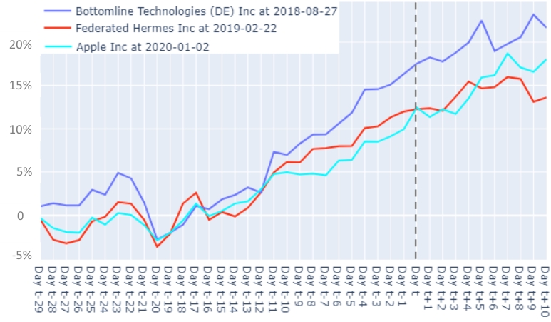
Although some previous work considers the interdependencies among different variables in the same timestamp, they overlook the inter-connections between a variable and other variables’ historical series. Due to the similar external environment or the periodicity of time series, a variable would have a similar series as other variables’ historical series. Figure 1 shows the cumulative return series of three stocks in different timestamps. Although there are not at identical timestamps, they still have similar time series, which implies that different variables at different timestamps would also have inter-dependencies. The inter-dependencies between historical time series and the current time series that we need to forecast are valuable. We can utilize these inter-dependencies and the historical time series of different variables to improve the multivariate time series forecasting.
In this paper, we propose a simple yet efficient instance-wise graph-based framework for multivariate time series forecasting (IGMTF), which utilizes the inter-dependencies between different variables at different time stamps. We first introduce the concept of series instance, which represents the observed values of a variable at a time stamp. Each series instance has a specific input series as the feature. Then we have the training instances in the training set and the mini-batch instances in each training/inference mini-batch. In general, the dataset’s training/validation/test sets are split by chronological order, so the training instances contain the historical series of different variables. We first use the training instance encoder and mini-batch instance encoder to encode the training and mini-batch instances. Then we utilize a training instances sampler to sample the most related training instances for each mini-batch as sample training instances. To capture the inter-dependencies between the historical series of different variables and the current series in the mini-batch, we construct an instance graph with the nodes of sampled training instances and mini-batch instances. The edges in instance graph are the connections between these two types of instances. Then we aggregate information from sampled training instances to mini-batch instances on the instance graph. Thus we can capture the inter-dependencies between the historical series of variables and the current series in mini-batch. Finally, we utilize aggregated information on mini-batch instances and the mini-batch instances’ information to forecast the time series.
We evaluate our framework on three multivariate time series benchmarks datasets: Traffic, Electricity, and Exchange-Rate. The experimental results show that our method outperforms existing multivariate time series methods. Moreover, the empirical analyses verify the effectiveness of some components and influence of some hyper-parameters in our IGMTF framework.
2 Related Work
In recent years, there have been many research efforts on multivariate time series forecasting problems. Some traditional linear regression methods include auto-regressive (AR), vector auto-regressive (VAR) (Zhang 2003), auto-regressive moving average (ARMA), auto-regressive integrated moving average (ARIMA) (Brown 2004), and support vector regression (SVR) (Cao and Tay 2003). They utilize the linear function of past time historical values to forecast the time series. Gaussian process (GP) (Roberts et al. 2013) is a Bayesian approach, modeling the distribution of a multivariate variable over functions, and can naturally apply to model multivariate time series data. Although traditional linear statistical models have the advantages of simplicity and interpretability, they have the limitation of strong assumptions with respect to a stationary process, and they do not scale well to multivariate time series data.
More recently, more and more deep learning based methods have been proposed because they are free from stationary assumptions and can capture the non-linearity patterns of series (Bai, Kolter, and Koltun 2018; Sen, Yu, and Dhillon 2019; Guo et al. 2019). One representative type of method is the recurrent neural networks (RNNs) and its variants such as long short-term memory (LSTM) (Hochreiter and Schmidhuber 1997) and gated recurrent units (GRU) (Chung et al. 2014). Some RNNs are specially designed for multivariate time series forecasting problems, such as LSTNet (Lai et al. 2018) and TPA-LSTM (Shih, Sun, and Lee 2019). The LSTNet utilizes convolutional neural networks (CNNs) to capture local dependencies among variables and RNNs to preserve the long-term temporal dependencies. The TPA-LSTM utilizes the attention mechanism to capture the long-term dependencies of multivariate time series. Nevertheless, the LSTNet and TPA-LSTM cannot fully exploit latent dependencies between pairs of variables. To capture the inter-dependencies among different variables in multivariate time series, MTGNN (Wu et al. 2020) and StemGNN (Cao et al. 2021) use the variables as nodes to construct a graph, and leverage graph neural networks (GNNs) (Kipf and Welling 2017) to mine the correlations among variables in the same time stamp.
However, previous multivariate time series forecasting methods overlook the inter-connections between different variables at different time stamps. Therefore, we propose an instance-wise graph-based framework to utilize the inter-dependencies between variables at different time stamps to boost multivariate time series forecasting.
Besides, some methods focus on the univariate time series forecasting problems (Patel et al. 2015; Rather, Agarwal, and Sastry 2015; Xingjian et al. 2015; Zhang, Aggarwal, and Qi 2017; Oreshkin et al. 2019; Montero-Manso et al. 2020). The main difference between univariate and multivariate time series forecasting methods is that univariate time series techniques analyze each time series separately without considering the correlations between different variables. Since considering correlations between different variables at different time series is the critical insight of our work, we do not introduce the univariate time series techniques in detail.
3 Preliminaries
In this section, we first formulate the problem of multivariate time series forecasting. Give a sequence observations on a multivariate variable at time stamp : , where is the length of input time stamps, and is the dimension of variables, our goal is to predict the future series value , where is the specified horizon ahead of the current timestamp. The horizon can be set to specific values according to the type of time series data. The multivariate time series forecasting is a rolling process. At timestamp , when we forecast the future value , we assume the sequence is available. Similarly, when we forecast the value at timestamp , we assume the sequence is available.
Besides, we would also describe the formal definition of some concepts in our framework below.
Definition 1.
Series Instance. A series instance is the observed values of a variable at timestamp . The feature of series instance is , where , and the forecasting label of series instance is . In this paper, we also call the series instance as instance for convenience.
In a multivariate time series, each variable at each timestamp would have a series instance. If a time series has 30 variables at 100 timestamps, then the number of series instances in this time series is 3000.
Definition 2.
Instance Graph. The instance graph is a graph whose nodes are the series instances. The edges are the similarity between different series instances.
4 Our Framework
This section elaborates on our proposed instance-wise graph-based framework for multivariate time series forecasting (IGMTF). Figure 2 shows the overall architecture of our framework. The key idea of our framework is capturing the interdependencies between historical instances of different variables and the current instances in the mini-batch. To achieve this goal, in Section 4.1 and 4.2, we first learn the embeddings of training and mini-batch instances. In Section 4.3, we use a training instance sampler to sample the most related training instances for each mini-batch. After that, in Section 4.4, we utilize the graph aggregation module to aggregate information from sampled training instances to mini-batch instances. Finally, in the forecasting module in Section 4.5, we use the aggregated information on mini-batch instances as well as the mini-batch instances’ embeddings to forecast the future time series.
4.1 Training Instances Encoder
The training instances encoder aims to learn the representations of series instances in training set , where and is the number of time stamps in the training set. At the beginning of each training epoch or model inference, we encode the features of all instances in . Since the feature of each instance is the historical values of a variable, we need to encode the historical information of each instance. The Gated Recurrent Unit (GRU) network (Chung et al. 2014) can capture the long-term dependency of series, so we feed the features of training instances in into a GRU. Then we further project the last hidden state of GRU’s output with a 3-layers MLP, and the output of MLP is the training instance embeddings , where and is the dimension of MLP’s output. In this MLP, there is a LeakyReLU (Maas, Hannun, and Ng 2013) activation function after each linear layer. It is noteworthy that we feed the training instances into the GRU and MLP in inference mode, without generating any gradients in this process.
4.2 Mini-batch Instances Encoder
The mini-batch instances encoder aims to learn the representations of series instances in a mini-batch . In our framework, each mini-batch is all the instances at the same time stamp, so the number of instances in a mini-batch equals the number of variables in the dataset. In each mini-batch , we feed the features of instances at time stamp into the same GRU in training instances encoder. We also feed the last hidden layer of GRU’s output to the same MLP in training instances encoder to make a projection. In the mini-batch instance encoder, the GRU and MLP are in training mode. They would generate gradients to update the parameters in GRU and MLP. The output of MLP , where , is the mibi-batch instance embeddings.
4.3 Training Instances Sampler
Since the number of training instances is huge and there is a vast computation cost to directly aggregate information from training instances to mini-batch instances, we utilize a training instances sampler to sample the most related training instances from for each mini-batch. We first calculate the mean value of training instance embeddings at each time stamp: , and the mean value mini-batch instance embeddings .
| (1) |
| (2) |
where is the mean embedding of training instances at time stamp , and is the mean embedding of mini-batch instance embeddings .
To find the most related instances for each mini-batch, we calculate the cosine similarity between each time stamp’s embedding and . We select the closest time stamp embeddings with according to the similarities. After that, we sample the training instances in these time stamps as sampled training time stamps. Since each time stamp has training instances, the total number of sampled training instances is . We would study the effect of training instances sampler in Section 5.4.
4.4 Graph Aggregation Module
In the graph aggregation module, we capture the inter-dependencies between the sampled training instances and the mini-batch instances . We first use the instances in and as nodes to construct a instance graph. In this instance graph, each sampled training instance and mini-batch instance are connected with an edge. Given sampled training instance embeddings and mini-batch instance embeddings , we aggregate the information from sampled training instances to mini-batch instances on the instance graph. Since the instance graph is not pre-defined and we do not know the weight between sampled training instances and mini-batch instances, we use the cosine similarity between sampled training instance embeddings and mini-batch instance embeddings as aggregated weights.
| (3) |
where and are two mapping matrices for and , respectively. We would study the effect of these two mapping matrices in Section 5.4. The is the similarity between mini-batch instance embedding and sampled training instance embedding , the matrix is the adjacent matrix from sampled training instances to mini-batch instances.
The current adjacent matrix indicates a fully connected graph since each training instance would calculate the similarity with each mini-batch instance. Some recent work (Li, Han, and Wu 2018; Liu, Gao, and Ji 2020) have pointed out that the deeper graph neural network (GNN) would cause the problem of over-smoothing, which is the repeated message propagation makes nodes in different classes have indistinguishable representations. Similarly, the GNN on a fully connected graph would also induce the issue of over-smoothing. Therefore, we introduce a top mask mechanism on the adjacent matrix . For the aggregated weights , where , from all training instances to the mini-batch instance , we only retain the top largest weights and mask the remaining weights as . In this way, we only retain the closest neighbors for each mini-batch instance. Then we utilize the masked adjacent matrix to aggregate information from the most closest training instances to each mini-batch instance:
| (4) |
where is the set of top closest training instances for the mini-batch instance . The is the information aggregation from the historical training instances to the instance at time stamp .
4.5 Forecasting Module
Finally, we combine aggregated information and mini-batch instances embedding to forecast the future time series jointly. We concatenate aggregation information from training instances and mini-batch instance embedding , and feed the concatenation into a linear layer. The dimensional output of linear layer is the time series forecasting , which is the prediction to the instance ’s label .
| (5) |
4.6 Model Training
We use stochastic gradient descent algorithm (SGD) with mini-batches to train our framework and leverage the Adam (Kingma and Ba 2015) for tuning the learning rate. We optimize our framework by minimizing the MAE loss function with L2 regularization:
| (6) |
where is the instances in a mini-batch, and are future series prediction and label of variable at time stamp . The is the regularization parameter, and represents all of the parameters in our framework. Algorithm 1 is the training algorithm of our framework.
5 Experiments
In this section, we present thorough empirical studies to evaluate and analyze our proposed IGMTF framework. We first introduce the datasets and experimental setting. Then we compare our IGMTF framework with exiting multivariate time series forecasting methods on the benchmark datasets. Moreover, we apply an ablation study to study the effect of some components in our framework. Finally, we analyze the influence of some parameters on our framework.
5.1 Datasets
We evaluate our method on the three multivariate time series forecasting benchmark datasets: Traffic, Electricity, and Exchange-Rate. All of these datasets are provided by (Lai et al. 2018). Table 1 shows the statistics of these three datasets. The detailed introduction of datasets are as follows:
- •
Traffic: the traffic dataset from the California Department of Transportation contains road occupancy rates measured by 862 sensors in San Francisco Bay area freeways during 2015 and 2016.
- •
Electricity: the electricity dataset from the UCI Machine Learning Repository contains electricity consumption for 321 clients from 2012 to 2014.
- •
Exchange-Rate: the exchange-rate dataset contains the daily exchange rates of eight foreign countries, including Australia, British, Canada, Switzerland, China, Japan, New Zealand, and Singapore, ranging from 1990 to 2016.
| Datasets | # Time | # Variables | Sample Rate |
|---|---|---|---|
| traffic | 17,544 | 862 | 1 hour |
| electricity | 26,304 | 321 | 1 hour |
| exchange-rate | 7,588 | 8 | 1 day |
Following (Lai et al. 2018; Wu et al. 2020), we split these three datasets into a training set (), validation set (), and test set () in chronological order. In these three datasets, the input feature length of an instance is 168 and the forecasting length is 1. Models are trained independently to forecast the target future step (horizon) 3, 6, 12, and 24.
5.2 Experimental Setting
Compared Methods
We compare our framework with the following multivariate time series forecasting methods:
- •
AR: A traditional auto-regressive model.
- •
VAR-MLP (Zhang 2003): A hybrid model of the vector auto-regressive model (VAR) and MLP.
- •
GP (Roberts et al. 2013): A Gaussian Process time series model.
- •
RNN-GRU (Chung et al. 2014): A recurrent neural network with fully connected GRU hidden units.
- •
LSTNet (Lai et al. 2018): A deep neural network that combines convolutional neural networks and recurrent neural networks to capture the long-term and short-term temporal patterns.
- •
TPA-LSTM (Shih, Sun, and Lee 2019): An attention-based recurrent neural network.
- •
MTGNN (Wu et al. 2020): A graph neural network based multivariate time series forecasting approach.
- •
MTGNN+sampling (Wu et al. 2020): The MTGNN model trained on a sampled subset in each iteration.
Evaluation Metrics
Following (Lai et al. 2018; Shih, Sun, and Lee 2019; Wu et al. 2020), we use the Root Relative Squared Error (RRSE) and Empirical Correlation Coefficient (CORR) as metrics to evaluate the forecasting results. The RRSE is a scaled version of the widely used Root Mean Square Error (RMSE), designed to make a more readable evaluation, regardless of the data scale. The lower RRSE value and higher CORR value indicate better performance.
| Dataset | ||||||||||
|---|---|---|---|---|---|---|---|---|---|---|
| Horizon | Horizon | |||||||||
| 3 | 6 | 12 | 24 | 3 | 6 | 12 | 24 | |||
| Traffic | 256 | 0.0001 | 30 | 5 | 10 | 3 | 20 | 30 | 30 | 10 |
| Electricity | 512 | 0.0001 | 5 | 3 | 10 | 5 | 20 | 3 | 5 | 20 |
| Exchange-Rate | 512 | 0.0001 | 20 | 5 | 10 | 5 | 20 | 10 | 10 | 20 |
| Dataset | Traffic | Electricity | Exchange-Rate | ||||||||||
|---|---|---|---|---|---|---|---|---|---|---|---|---|---|
| Methods | Metrics | Horizon | Horizon | Horizon | |||||||||
| 3 | 6 | 12 | 24 | 3 | 6 | 12 | 24 | 3 | 6 | 12 | 24 | ||
| AR | RRSE () | 0.5991 | 0.6218 | 0.6252 | 0.63 | 0.0995 | 0.1035 | 0.1050 | 0.1054 | 0.0228 | 0.0279 | 0.0353 | 0.0445 |
| CORR () | 0.7752 | 0.7568 | 0.7544 | 0.7519 | 0.8845 | 0.8632 | 0.8591 | 0.8595 | 0.9734 | 0.9656 | 0.9526 | 0.9357 | |
| VARMLP | RRSE () | 0.5582 | 0.6579 | 0.6023 | 0.6146 | 0.1393 | 0.1620 | 0.1557 | 0.1274 | 0.0265 | 0.0394 | 0.0407 | 0.0578 |
| CORR () | 0.8245 | 0.7695 | 0.7929 | 0.7891 | 0.8708 | 0.8389 | 0.8192 | 0.8679 | 0.8609 | 0.8725 | 0.8280 | 0.7675 | |
| GP | RRSE () | 0.6082 | 0.6772 | 0.6406 | 0.5995 | 0.1500 | 0.1907 | 0.1621 | 0.1273 | 0.0239 | 0.0272 | 0.0394 | 0.0580 |
| CORR () | 0.7831 | 0.7406 | 0.7671 | 0.7909 | 0.8670 | 0.8334 | 0.8394 | 0.8818 | 0.8713 | 0.8193 | 0.8484 | 0.8278 | |
| RNN-GRU | RRSE () | 0.5358 | 0.5522 | 0.5562 | 0.5633 | 0.1102 | 0.1144 | 0.1183 | 0.1295 | 0.0192 | 0.0264 | 0.0408 | 0.0626 |
| CORR () | 0.8511 | 0.8405 | 0.8345 | 0.8300 | 0.8597 | 0.8623 | 0.8472 | 0.8651 | 0.9786 | 0.9712 | 0.9531 | 0.9223 | |
| LSTNet-skip | RRSE () | 0.4777 | 0.4893 | 0.4950 | 0.4973 | 0.0864 | 0.0931 | 0.1007 | 0.1007 | 0.0226 | 0.0280 | 0.0356 | 0.0449 |
| CORR () | 0.8721 | 0.8690 | 0.8614 | 0.8588 | 0.9283 | 0.9135 | 0.9077 | 0.9119 | 0.9735 | 0.9658 | 0.9511 | 0.9354 | |
| TPA-LSTM | RRSE () | 0.4487 | 0.4658 | 0.4641 | 0.4765 | 0.0823 | 0.0916 | 0.0964 | 0.1006 | 0.0174 | 0.0241 | 0.0341 | 0.0444 |
| CORR () | 0.8812 | 0.8717 | 0.8717 | 0.8629 | 0.9439 | 0.9337 | 0.9250 | 0.9133 | 0.9790 | 0.9709 | 0.9564 | 0.9381 | |
| MTGNN | RRSE () | 0.4162 | 0.4754 | 0.4461 | 0.4535 | 0.0745 | 0.0878 | 0.0916 | 0.0953 | 0.0194 | 0.0259 | 0.0349 | 0.0456 |
| CORR () | 0.8963 | 0.8667 | 0.8794 | 0.8810 | 0.9474 | 0.9316 | 0.9278 | 0.9234 | 0.9786 | 0.9708 | 0.9551 | 0.9372 | |
| MTGNN | RRSE () | 0.4170 | 0.4435 | 0.4469 | 0.4537 | 0.0762 | 0.0862 | 0.0938 | 0.0976 | 0.0212 | 0.0271 | 0.0350 | 0.0454 |
| +sampling | CORR () | 0.8960 | 0.8815 | 0.8793 | 0.8758 | 0.9467 | 0.9354 | 0.9261 | 0.9219 | 0.9788 | 0.9704 | 0.9574 | 0.9382 |
| IGMTF | RRSE () | 0.4135 | 0.4319 | 0.4422 | 0.4471 | 0.0740 | 0.0851 | 0.0930 | 0.0983 | 0.0173 | 0.0239 | 0.0329 | 0.0427 |
| CORR () | 0.8978 | 0.8879 | 0.8825 | 0.8796 | 0.9508 | 0.9404 | 0.9311 | 0.9240 | 0.9796 | 0.9718 | 0.9577 | 0.9391 | |
| Dataset | Traffic | Electricity | |||||||
|---|---|---|---|---|---|---|---|---|---|
| Metrics | Methods | Horizon | Horizon | ||||||
| 3 | 6 | 12 | 24 | 3 | 6 | 12 | 24 | ||
| RRSE () | IGMTF_NS | 0.4172 | 0.4591 | 0.4466 | 0.4515 | 0.0756 | 0.0863 | 0.0955 | 0.0994 |
| IGMTF_NW | 0.4185 | 0.4366 | 0.4456 | 0.4512 | 0.0746 | 0.0865 | 0.0943 | 0.1005 | |
| IGMTF | 0.4135 | 0.4319 | 0.4422 | 0.4471 | 0.0740 | 0.0851 | 0.0930 | 0.0983 | |
| CORR () | IGMTF_NS | 0.8963 | 0.8757 | 0.8797 | 0.8766 | 0.9494 | 0.9384 | 0.9295 | 0.9234 |
| IGMTF_NW | 0.8958 | 0.8862 | 0.8808 | 0.8772 | 0.9501 | 0.9390 | 0.9301 | 0.9229 | |
| IGMTF | 0.8978 | 0.8879 | 0.8825 | 0.8796 | 0.9508 | 0.9404 | 0.9311 | 0.9240 | |
Implementation Details
We implement our framework base on the PyTorch library (Paszke et al. 2019)11 1 Our source code and data are available at this repository: https://github.com/Wentao-Xu/IGMTF., and run on all experiments with a single NVIDIA Tesla V100 GPU. We tune our framework using the grid search to select the optimal hyper-parameters based on the performance of the validation set. We search the number of hidden units in GRU and MLP in {128, 256, 512, 1024}; the number of closest time stamps (in training instance sampler) and the number of closest neighbors (in graph aggregation module) in {3, 5, 10, 20, 30}; the learning rate in {0.002, 0.001, 0.0005, 0.0001, 0.00005}. Table 2 list the best selections of hyper-parameters on different datasets and horizons. Besides, as point out in Section 4.2, the batch size of our framework is the number of instances on each time stamp, and the number of training epoch is for all datasets.
5.3 Main Results
Table 3 shows the results of RRSE and CORR on Traffic, Electricity, and Exchange-Rate datasets. On the RRSE metrics, our framework achieves the best results on the Electricity dataset when the horizon is 3 and 6, and the best results on Traffic and Exchange-Rate in all horizons. On the CORR metrics, our frame outperforms the compared methods except for the Traffic dataset when the horizon is 24. Although on some metrics in some horizons, our IGMTF framework is worse than MTGNN or MTGNN+sampling, the IGMTF still performs better than the rest of the baselines.
The results in Table 3 verify the effectiveness of our IGMTF framework. In most cases, our framework is better than MTGNN, which utilizes the graph neural network to mine the inter-dependencies among variables in the same time stamp. Compared with MTGNN, our IGMTF can utilize the correlations between different variables in different time stamps. Therefore, capturing the interdependencies between different variables in different time stamps can further improve multivariate time series forecasting performance.
5.4 Ablation Study
We apply an ablation study to study the effect of some components in our framework, including the training instance sampler in Section 4.3 and the mapping matrices and of graph aggregation module in Section 4.4. To study the effect of these two components, we compare our IGMTF framework with the following IGMTF’ variants:
- •
IGMTF_NS: To study the effect of the training instance sampler in Section 4.3, the IGMTF_NS remove the training instance sampler and randomly sample the same number of instances as sampled training instances.
- •
IGMTF_NW: To study the effect of the mapping matrices and of graph aggregation module in Section 4.4, the IGMTF_NW remove and from the IGMTF framework.
Table 4 shows the results of IGMTF_NS, IGMTF_NW, and IGMTF at Traffic and Electricity datasets. From Table 4 we can find that removing the training instance sampler or matrices and of the graph aggregation module would both reducing the performance of the IGMTF framework. Specifically, without a training instance sampler, our IGMTF framework would significantly weaken the forecasting results on the Traffic dataset with a horizon of 6. These results illustrate the training instance sampler is vital for our IGMTF framework to sample the most related instances for mini-batch instances from all training instances. The ablation study results also verify that the mapping matrices in the graph aggregation module are necessary and can improve the performance of our framework.
5.5 Hyper-parameters Analysis
In the training instance sampler, we have a hyper-parameter to control the number of time stamps we sample from the training instances. Meanwhile, there is also a hyper-parameter in the graph aggregation module to select the number of neighbors to aggregate information from sampled training instances to each mini-batch instance. In this subsection, we will study the influence of hyper-parameters and on the performance of our IGMTF framework.
Influence of the Number of Closest Time Stamps
We let vary in {3, 5, 10, 20, 30}, and we set the hyper-parameter as 10 and fix all the other hyper-parameters. Then we observe the RRSE and CORR results on Traffic and Electricity datasets under different . Figure 3 shows the results under different . The influence of is more significant on the Traffic dataset than the Electricity dataset. On the Traffic dataset, IGMTF achieves the best results at horizons 3, 6, 12, 24 when is 30, 5, 10, 3, respectively. On the Electricity dataset, IGMTF achieves the best results at horizons 3, 6, 12, 24 when is 5, 3, 10, 5, respectively.

Influence of the Number of Closest Neighbors
We let vary in {3, 5, 10, 20, 30}, and we set the hyper-parameter as 10 and fix all the other hyper-parameters. Then we observe the RRSE and CORR results on Traffic and Electricity datasets under different . Figure 4 shows the results under different . On the Traffic dataset, IGMTF achieves the best results at horizons 3, 6, 12, 24 when is 20, 30, 30, 10, respectively. On the Electricity dataset, IGMTF achieves the best results at horizons 3, 6, 12, 24 when is 20, 3, 5, 20, respectively.
The influence of the numbers of closest time stamps and neighbors suggest that both the and are sensitive hyper-parameters that need to be tuned for the best performance given a dataset and a horizon.
6 Conclusion and Future Work
In this work, we propose a simple yet efficient instance-wise graph-based framework (IGMTF) for multivariate time series forecasting. Our framework can address exiting work’s limitation that overlooks the interdependencies between different variables at different time stamps. The key idea of our framework to address this limitation is aggregating information from historical training instances to mini-batch instances. We evaluate our framework on the multivariate time series benchmark datasets. The experimental results show that our proposed model performs better than the state-of-the-art baseline methods.
In the future, we plan the explore more techniques, such as contrastive learning, to mine valuable interdependences between different time series at different time stamps.
References
- Bai, Kolter, and Koltun (2018) Bai, S.; Kolter, J. Z.; and Koltun, V. 2018. An empirical evaluation of generic convolutional and recurrent networks for sequence modeling. arXiv preprint arXiv:1803.01271.
- Brown (2004) Brown, R. G. 2004. Smoothing, forecasting and prediction of discrete time series. Courier Corporation.
- Cao et al. (2021) Cao, D.; Wang, Y.; Duan, J.; Zhang, C.; Zhu, X.; Huang, C.; Tong, Y.; Xu, B.; Bai, J.; Tong, J.; et al. 2021. Spectral temporal graph neural network for multivariate time-series forecasting. arXiv preprint arXiv:2103.07719.
- Cao and Tay (2003) Cao, L.-J.; and Tay, F. E. H. 2003. Support vector machine with adaptive parameters in financial time series forecasting. IEEE Transactions on neural networks, 14(6): 1506–1518.
- Chung et al. (2014) Chung, J.; Gulcehre, C.; Cho, K.; and Bengio, Y. 2014. Empirical evaluation of gated recurrent neural networks on sequence modeling. arXiv preprint arXiv:1412.3555.
- Guo et al. (2019) Guo, S.; Lin, Y.; Feng, N.; Song, C.; and Wan, H. 2019. Attention based spatial-temporal graph convolutional networks for traffic flow forecasting. In Proceedings of the AAAI Conference on Artificial Intelligence, volume 33, 922–929.
- Hochreiter and Schmidhuber (1997) Hochreiter, S.; and Schmidhuber, J. 1997. Long short-term memory. Neural computation, 9(8): 1735–1780.
- Kingma and Ba (2015) Kingma, D. P.; and Ba, J. 2015. Adam: A method for stochastic optimization. In International Conference on Learning Representations (ICLR).
- Kipf and Welling (2017) Kipf, T. N.; and Welling, M. 2017. Semi-Supervised Classification with Graph Convolutional Networks. In International Conference on Learning Representations (ICLR).
- Lai et al. (2018) Lai, G.; Chang, W.-C.; Yang, Y.; and Liu, H. 2018. Modeling long-and short-term temporal patterns with deep neural networks. In The 41st International ACM SIGIR Conference on Research & Development in Information Retrieval, 95–104.
- Li, Han, and Wu (2018) Li, Q.; Han, Z.; and Wu, X.-M. 2018. Deeper insights into graph convolutional networks for semi-supervised learning. In Thirty-Second AAAI conference on artificial intelligence.
- Liu, Gao, and Ji (2020) Liu, M.; Gao, H.; and Ji, S. 2020. Towards deeper graph neural networks. In Proceedings of the 26th ACM SIGKDD International Conference on Knowledge Discovery & Data Mining, 338–348.
- Maas, Hannun, and Ng (2013) Maas, A. L.; Hannun, A. Y.; and Ng, A. Y. 2013. Rectifier nonlinearities improve neural network acoustic models. In Proc. icml, volume 30, 3. Citeseer.
- Montero-Manso et al. (2020) Montero-Manso, P.; Athanasopoulos, G.; Hyndman, R. J.; and Talagala, T. S. 2020. FFORMA: Feature-based forecast model averaging. International Journal of Forecasting, 36(1): 86–92.
- Oreshkin et al. (2019) Oreshkin, B. N.; Carpov, D.; Chapados, N.; and Bengio, Y. 2019. N-BEATS: Neural basis expansion analysis for interpretable time series forecasting. arXiv preprint arXiv:1905.10437.
- Paszke et al. (2019) Paszke, A.; Gross, S.; Massa, F.; Lerer, A.; Bradbury, J.; Chanan, G.; Killeen, T.; Lin, Z.; Gimelshein, N.; Antiga, L.; et al. 2019. Pytorch: An imperative style, high-performance deep learning library. arXiv preprint arXiv:1912.01703.
- Patel et al. (2015) Patel, J.; Shah, S.; Thakkar, P.; and Kotecha, K. 2015. Predicting stock market index using fusion of machine learning techniques. Expert Systems with Applications, 42(4): 2162–2172.
- Rather, Agarwal, and Sastry (2015) Rather, A. M.; Agarwal, A.; and Sastry, V. 2015. Recurrent neural network and a hybrid model for prediction of stock returns. Expert Systems with Applications, 42(6): 3234–3241.
- Roberts et al. (2013) Roberts, S.; Osborne, M.; Ebden, M.; Reece, S.; Gibson, N.; and Aigrain, S. 2013. Gaussian processes for time-series modelling. Philosophical Transactions of the Royal Society A: Mathematical, Physical and Engineering Sciences, 371(1984): 20110550.
- Sen, Yu, and Dhillon (2019) Sen, R.; Yu, H.-F.; and Dhillon, I. 2019. Think globally, act locally: A deep neural network approach to high-dimensional time series forecasting. arXiv preprint arXiv:1905.03806.
- Shih, Sun, and Lee (2019) Shih, S.-Y.; Sun, F.-K.; and Lee, H.-y. 2019. Temporal pattern attention for multivariate time series forecasting. Machine Learning, 108(8): 1421–1441.
- Wu et al. (2020) Wu, Z.; Pan, S.; Long, G.; Jiang, J.; Chang, X.; and Zhang, C. 2020. Connecting the dots: Multivariate time series forecasting with graph neural networks. In Proceedings of the 26th ACM SIGKDD International Conference on Knowledge Discovery & Data Mining, 753–763.
- Xingjian et al. (2015) Xingjian, S.; Chen, Z.; Wang, H.; Yeung, D.-Y.; Wong, W.-K.; and Woo, W.-c. 2015. Convolutional LSTM network: A machine learning approach for precipitation nowcasting. In Advances in neural information processing systems, 802–810.
- Zhang (2003) Zhang, G. P. 2003. Time series forecasting using a hybrid ARIMA and neural network model. Neurocomputing, 50: 159–175.
- Zhang, Aggarwal, and Qi (2017) Zhang, L.; Aggarwal, C.; and Qi, G.-J. 2017. Stock price prediction via discovering multi-frequency trading patterns. In Proceedings of the 23rd ACM SIGKDD International Conference on Knowledge Discovery and Data Mining, 2141–2149. ACM.