Tian Li∗, Ahmad Beirami∗, Maziar Sanjabi, Virginia Smith
On Tilted Losses in Machine Learning:
Theory and Applications
Abstract
Exponential tilting is a technique commonly used in fields such as statistics, probability, information theory, and optimization to create parametric distribution shifts. Despite its prevalence in related fields, tilting has not seen widespread use in machine learning. In this work, we aim to bridge this gap by exploring the use of tilting in risk minimization. We study a simple extension to ERM—tilted empirical risk minimization (TERM)—which uses exponential tilting to flexibly tune the impact of individual losses. The resulting framework has several useful properties: We show that TERM can increase or decrease the influence of outliers, respectively, to enable fairness or robustness; has variance-reduction properties that can benefit generalization; and can be viewed as a smooth approximation to the tail probability of losses. Our work makes connections between TERM and related objectives, such as Value-at-Risk, Conditional Value-at-Risk, and distributionally robust optimization (DRO). We develop batch and stochastic first-order optimization methods for solving TERM, provide convergence guarantees for the solvers, and show that the framework can be efficiently solved relative to common alternatives. Finally, we demonstrate that TERM can be used for a multitude of applications in machine learning, such as enforcing fairness between subgroups, mitigating the effect of outliers, and handling class imbalance. Despite the straightforward modification TERM makes to traditional ERM objectives, we find that the framework can consistently outperform ERM and deliver competitive performance with state-of-the-art, problem-specific approaches.
keywords
Exponential tilting, empirical risk minimization, Value-at-Risk, superquantile optimization, fairness, robustness.1 Introduction
Many statistical estimation procedures rely on the concept of empirical risk minimization (ERM), in which the parameter of interest, , is estimated by minimizing an average loss over the data :
| (1) |
Although ERM is widely used in machine learning, it is known to perform poorly in situations where average performance is not an appropriate surrogate for the problem of interest. Significant research has thus been devoted to developing alternatives to traditional ERM for diverse applications, such as learning in the presence of noisy/corrupted data (Khetan et al. 2018; Jiang et al. 2018), performing classification with imbalanced data (Lin et al. 2017; Malisiewicz et al. 2011), ensuring that subgroups within a population are treated fairly (Hashimoto et al. 2018; Samadi et al. 2018), or developing solutions with favorable out-of-sample performance (Duchi and Namkoong 2019).
In this paper, we suggest that deficiencies in ERM can be flexibly addressed via a unified framework, tilted empirical risk minimization (TERM). TERM encompasses a family of objectives, parameterized by a real-valued hyperparameter, . For the -tilted loss (TERM objective) is given by:
| (2) |
TERM generalizes ERM as the -tilted loss recovers the average loss, i.e., .11 1 is defined in (20) via the continuous extension of . It also recovers other popular alternatives such as the max-loss () and min-loss () (Lemma 4). As we discuss below, although tilted risk minimization is not widely used in machine learning, variants of tilting have been extensively studied in related fields including statistics, applied probability, optimization, and information theory.
1.1 Perspectives on Exponential Tilting
We begin by defining exponential tilting and discussing uses of tilting in various fields. Let be a set of parametric distributions. For any , we let be the information of under , which is defined as (Cover and Thomas 1991):
| (3) |
Further assume that is a random variable drawn from distribution which is not necessarily matched to , i.e., the model family may be misspecified. The cumulant generating function of the information random variable, can be stated as (Dembo and Zeitouni 2009, Section 2.2):
| (4) |
where in this paper denotes expectation with respect to the true distribution unless otherwise stated. This expectation is commonly referred to as an exponential tilt of the information density, and can induce parametric distribution shifts that have varied applications in probability, statistics, and information theory. In particular, it is noteworthy that if is an exponential family of distributions parameterized by then the tilted distribution (when normalized by ) also belongs to the same exponential family. Further, given samples the empirical cumulant generating function is defined as:
| (5) |
It is thus evident that TERM (2) can be viewed as an appropriately scaled variant of the empirical cumulant generating function in (5). Although tilting of this form has been used in a number of related disciplines, uses of exponential tilting in machine learning are relatively unexplored. We provide several perspectives on exponential tilting from other fields below.
Statistics.
Exponential tilting is well-known as a distribution shifting technique in statistics, where the main idea is to draw samples from an exponentially tilted version of the original distribution to improve the convergence properties of statistical estimation, especially when the distribution of interest belongs to an exponential family, such as Gaussian or multinomial. Common use cases include rejection sampling, rare-event simulation, saddle-point approximation (Butler 2007, p. 156), and importance sampling (Siegmund 1976).
Applied probability.
In large deviations theory, exponential tilting lies at the heart of deriving concentration bounds. For example, Chernoff bounds apply Markov’s inequality to which results in a parametric set of bounds by using exponential tilts of various orders. The bound may then be further optimized on the real tilt value to derive the tightest possible bound (Dembo and Zeitouni 2009).
Information theory.
While source coding limits and channel capacity are characterized by Shannon entropy and Shannon mutual information (which are simple averages over the information (3)) (Cover and Thomas 1991), there are other elements of information theory that are not characterized by the average, such as error exponents in channel decoding (Gallager 1968), probability of error in list decoding (Merhav 2014), and computational cost in sequential decoding (Massey 1994; Arıkan 1996). These fundamental elements of information theory are asymptotically determined by a non-zero tilted cumulant generating function of the information random variable (3) (see (Beirami et al. 2018) for further discussion).
Optimization.
Exponential tilting has also appeared as a minimax smoothing approach in optimization (Kort and Bertsekas 1972; Pee and Royset 2011; Liu and Theodorou 2019). Such smooth approximations to the max often appear through LogSumExp functions, with applications in geometric programming (Calafiore and El Ghaoui 2014, Sec. 9.7), and boosting (Mason et al. 1999; Shen and Li 2010). We discuss min-max objectives and the connections with TERM in several subsequent sections of the paper.
Machine learning.
Despite the rich history of tilted objectives in related fields, they have not seen widespread use in ML beyond limited applications such as robust regression (Wang et al. 2013) and sequential decision making (Howard and Matheson 1972; Borkar 2002). In this work, we argue that tilting is a critical yet undervalued tool in machine learning. We demonstrate the effectiveness of tilting by (i) rigorously studying properties of the TERM objective, and (ii) exploring its utility for a wide range of ML applications. Surprisingly, we find that this simple extension to ERM can match or exceed state-of-the-art performance from highly tuned, bespoke solutions to common ML problems, from learning with noisy data to ensuring fair performance between subgroups. We highlight several motivating applications of TERM below and provide an outline of the remainder of the paper in Section 1.3.
1.2 Motivating Examples
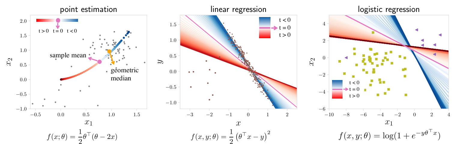
To motivate how the TERM objective (2) may be used in machine learning, we provide several running examples below, which are illustrated in Figure 1.
(a) Point estimation: As a first example, consider determining a point estimate from a set of samples that contain some outliers. We plot an example 2D dataset in Figure 1a, with data centered at (1,1). Using traditional ERM (i.e., TERM with ) recovers the sample mean, which can be biased towards outlier data. By setting , TERM can suppress outliers by reducing the relative impact of the largest losses (i.e., points that are far from the estimate) in (2). A specific value of can in fact approximately recover the geometric median, as the objective in (2) can be viewed as approximately optimizing specific loss quantiles (a connection which we make explicit in Section 2). In contrast, if these ‘outlier’ points are important to estimate, setting will push the solution towards a point that aims to minimize variance, as we prove in Section 2, Theorem 33.
(b) Linear regression: A similar interpretation holds for the case of linear regression (Figure 2b). As TERM finds a line of best while ignoring outliers. However, this solution may not be preferred if we have reason to believe that these ‘outliers’ should not be ignored. As TERM recovers the min-max solution, which aims to minimize the worst loss, thus ensuring the model is a reasonable fit for all samples (at the expense of possibly being a worse fit for many). Similar criteria have been used, e.g., in defining notions of fairness (Hashimoto et al. 2018; Samadi et al. 2018). We explore several use-cases involving robust regression and fairness in more detail in Section 7.
(c) Logistic regression: Finally, we consider a binary classification problem using logistic regression (Figure 2c). For , the TERM solution varies from the nearest cluster center (), to the logistic regression classifier (), towards a classifier that magnifies the misclassified data (). We note that it is common to modify logistic regression classifiers by adjusting the decision threshold from , which is equivalent to moving the intercept of the decision boundary. This is fundamentally different than what is offered by TERM (where the slope is changing). As we show in Section 7, this added flexibility affords TERM with competitive performance on a number of classification problems, such as those involving noisy data, class imbalance, or a combination of the two.
1.3 Contributions
In this work, we explore the use of tilting in machine learning through TERM, a simple, unified framework that can flexibly address various challenges with empirical risk minimization. We first analyze the objective and its solutions, showcasing the behavior of TERM with varying tilt parameters (Section 2). We also establish connections between TERM and related approaches such as distributionally robust optimization in Section 3.
We rigorously analyze the relations between TERM and other risks (e.g, Value-at-Risk (VaR), Conditional Value-at-Risk (CVaR), and Entropic Value-at-Risk (EVaR)) in Section 4. In particular, we introduce a new risk measure based on TERM, called Tilted Value-at-Risk (TiVaR), to approximate VaR. We show that TiVaR can provide a better approximation of VaR than CVaR in certain regimes, and improves upon EVaR in all regimes.
We develop efficient first-order batch and stochastic methods for solving TERM, both for hierarchical and non-hierarchical cases (Section 5 and 6). We provide convergence rates scaling with the hyperparameter on both convex and non-convex problems for both batch and stochastic algorithms. Our solvers run within 2–3 wall-clock time compared with that of ERM in all explored case studies.
Finally, we show via numerous case studies that TERM is competitive with existing, problem-specific state-of-the-art solutions (Section 7). We also extend TERM to handle compound issues, such as the simultaneous existence of noisy samples and imbalanced classes (Section 6). Our results demonstrate the effectiveness and versatility of tilted objectives in machine learning.
We note that the material in this paper was presented in part at ICLR 2021 (Li and Beirami et al., 2021). Compared to this earlier work, the current manuscript provides additional historical background of tilting (Section 1), establishes stronger and novel relationships between tilted losses and other risk-averse objectives in the literature (Section 3 and Section 4), provides convergence guarantees for our stochastic solver of TERM (Section 5), offers comprehensive details on applications of the framework in practice, and considers new applications of TERM to meta-learning and heteroskedastic deep learning (Section 7).
Outline.
This paper is organized as follows. We discuss general properties and interpretations of TERM in Section 2. We connect TERM with other prior risk measures in Section 3 and propose a new risk motivated by TERM in Section 4. In Section 5, we develop both batch and stochastic algorithms for optimizing TERM and provide convergence guarantees for them. We extend TERM to hierarchical multi-objective tilting in Section 6 and demonstrate the flexibility and competitive performance of the TERM framework via real-world applications in Section 7. We discuss related work in Section 8 and conclude the paper with Section 9.
2 TERM: Properties and Interpretations
To better understand the performance of the -tilted losses in (2), in this section we provide several interpretations of the TERM solutions, leaving the full proofs to the appendix. We make no distributional assumptions on the data, and study properties of TERM under the assumption that the loss function forms a generalized linear model, e.g., loss and logistic loss. However, we also obtain favorable empirical results using TERM with other objectives such as PCA and deep neural networks in Section 7, motivating the extension of this part of our theory beyond GLMs in future work.
2.1 Assumptions
We first provide notation and assumptions that are used throughout our theoretical analyses. The results in this paper are derived under one of the following three nested assumptions (the assumptions become progressively more restrictive, i.e., ):
Assumption 1 (Continuous differentiability).
For the loss function belongs to the differentiability class (i.e., continuously differentiable) with respect to
Assumption 2 (Smoothness and strong convexity condition).
Assume that Assumption 1 is satisfied. In addition, for any , belongs to differentiability class (i.e., twice differentiable with continuous Hessian) with respect to . We further assume that there exist such that for and any
| (6) |
where is the identity matrix of appropriate size (in this case ), and there does not exist any such that for all
Assumption 3 (Generalized linear model condition (Wainwright and Jordan 2008)).
Assume that Assumption 2 is satisfied. Further, assume that the loss function is given by
| (7) |
where is a convex function such that there exists where for any
| (8) |
and
| (9) |
This set of assumptions become the most restrictive with Assumption 3, which essentially requires that the loss be the negative log-likelihood of an exponential family. While the assumption is stated using the natural parameter of an exponential family for ease of presentation, the results hold for any bijective and smooth reparameterization of the exponential family. For example, Assumption 3 is satisfied by the commonly used loss for regression and logistic loss for classification (see toy examples (b) and (c) in Figure 1). assumes a reasonable regularity on the dataset . For instance, in the case of linear regression (), it reduces to the standard regularity assumption (where ). While Assumption 3 is not satisfied when we use neural network function approximators in Section 7, we observe favorable numerical results motivating the extension of these results beyond the cases that are theoretically studied in this paper.
In the sequel, many of the results are concerned with characterizing the -tilted solutions defined as the parametric set of solutions of -tiled losses by sweeping ,
| (10) |
where is an open subset of Further, let the optimal tilted objective be defined as
| (11) |
We state a final assumption, on , below.
Assumption 4 (Strict saddle property (Definition 4 in Ge et al. 2015)).
We assume that the set is non-empty for all . Further, we assume that for all is a “strict saddle” as a function of , i.e., for all local minima, , and for all other stationary solutions, , where is the minimum eigenvalue of the matrix.
We use the strict saddle property in order to reason about the properties of the -tilted solutions. In particular, since we are solely interested in the local minima of the strict saddle property implies that for every for a sufficiently small , for all
| (12) |
where denotes a -ball of radius around We will show later in Section 2.2 that the strict saddle property is readily verified for under Assumption 2, and we need Assumption 4 to be able to reason about .
2.2 General Properties of TERM
We begin by noting several general properties of the TERM objective (2). In particular: (i) is -Lipschitz continuous in if is -Lipschitz (Lemma 1); (ii) If is strongly convex, the -tilted loss is strongly convex for (Lemma 2); and (iii) Given a smooth , the -tilted loss is smooth for all finite (Lemma 3). We state these properties more formally below.
Lemma 0 (Lipschitzness of ).
For any and , if for , is -Lipschitz conditnuous in , then is -Lipschitz in .
Lemma 0 (Tilted Hessian and strong convexity for ).
Under Assumption 2, for any
| (13) | ||||
| (14) |
In particular, for all and all the -tilted objective is strongly convex. That is
| (15) |
Lemma 1 and 2 are proved in Appendix A. Lemma 2 also implies that under Assumption 2, the strict saddle assumption (Assumption 4) is readily verified.
Lemma 0 (Smoothness of ).
For any , let be the smoothness parameter of twice differentiable :
| (16) |
where is the Hessian of at and denotes the largest eigenvalue. Under Assumption 2, for any is a -smooth function of . Further, for 22 2 denotes the set of non-positive real numbers.
| (17) |
where is defined in Assumption 2. For
| (18) |
Lemma 3 (proved in Appendix A.1) indicates that -tilted losses are -smooth for all . is bounded for all negative and moderately positive , whereas it scales linearly with as , which has been previously studied in the context of exponential smoothing of the max (Kort and Bertsekas 1972; Pee and Royset 2011). This can also be observed visually via the toy example in Figure 2.
As discussed in Section 1, TERM can recover traditional ERM (), the max-loss (), and the min-loss (). We formally state this in Lemma 4 below.
Lemma 0.
Under Assumption 1,
| (19) | ||||
| (20) | ||||
| (21) |
where is the max-loss and is the min-loss33 3 When the argument of the max-loss or the min-loss is not unique, for the purpose of differentiating the loss function, we define as the average of the individual losses that achieve the maximum, and as the average of the individual losses that achieve the minimum.:
| (22) |
Note that Lemma 4 has been studied or observed before in the entropic risk literature (Ahmadi-Javid 2012, e.g.,), as well as other contexts (Cohen and Shashua 2014). This lemma also implies that is the ERM solution, is the min-max solution, and is the min-min solution. In other words, a benefit of TERM is that it offers a continuum of solutions between the min and max losses.
Providing a smooth trade-off between these specific losses can be beneficial for a number of practical use-cases—both in terms of the resulting solution and the difficulty of solving the problem itself. We empirically demonstrate the benefits of such a trade-off in Section 7. We also visualize the solutions to TERM for a toy problem in Figure 2, which allows us to illustrate several special cases of the general framework. Interestingly, we additionally show that the TERM solution can be viewed as a smooth approximation to the tail probability of losses, which effectively minimizes quantiles of losses such as the median loss (Section 4). In Figure 2, it is clear to see why this may be beneficial, as the median loss (orange) can be highly non-smooth in practice. In Theorem 5 and 6 below, we formally characterize how tilted objectives change as a function of values (proofs provided in Appendix A).
Theorem 5 (Tilted objective is increasing with ).
Under Assumption 3, for all and all
| (23) |
Theorem 6 (Optimal tilted objective is increasing with ).
Under Assumption 3, for all and all
| (24) |
Recall that TERM as and corresponds to min-loss and max-loss, respectively. We discuss in Section 4.2 that solving TERM with any can indeed be viewed as approximately minimizing the -th smallest loss () among all individual losses. As we increase from to the corresponding value of sweeps in . Theorem 6 hence roughly states that the optimal -th smallest loss is non-decreasing with , which is intuitively expected.
We next provide two interesting interpretations of the TERM framework to further understand its behavior.
2.3 Interpretation 1: Re-Weighting Samples to Magnify/Suppress Outliers
As discussed via the toy examples in Section 1, TERM can be tuned (using ) to magnify or suppress the influence of outliers. We make this notion rigorous by exploring the gradient of the -tilted loss in order to reason about the solutions to the objective defined in (2).
Lemma 0 (Tilted gradient).
For a smooth loss function ,
| (25) |
where tilted weights are given by
| (26) |
Under Assumption 1, we have:
| (27) |
Lemma 7 provides the gradient of the tilted objective, which has been studied previously in the context of exponential smoothing (see Pee and Royset 2011). From this, we can observe that the tilted gradient is a weighted average of the gradients of the original individual losses, where each data point is weighted exponentially proportional to the value of its loss. Note that recovers the uniform weighting associated with ERM, i.e., . For positive this has the effect of magnifying the outliers—samples with large losses—by assigning more weight to them, and for negative it suppresses the outliers by assigning less weight to them (Figure 3).
Generalizing the notion of tilted gradients (weighted average of individual gradients), we define tilted empirical mean over any -vector below, which will be used throughout the paper.
Definition 0 (Tilted empirical mean and variance).
For , let weighted empirical mean with weights (where stands for dimensional simplex) be defined as
| (28) |
Tilted empirical mean is weighted empirical mean with tilted weights, i.e.,
| (29) | ||||
| (30) |
where is defined in Eq. (26), and is defined in Eq. (10). We also refer to as the “-tilted empirical mean”. Similarly, tilted empirical variance is defined as
| (31) | ||||
| (32) |
and we refer to as the “-tilted empirical variance”.
As discussed before, the full gradient of TERM is tilted empirical mean of individual gradients with weights proportional to . In the next section as well as Appendix A.3, we will prove other properties of TERM using tilted empirical mean and variance defined here.
2.4 Interpretation 2: Empirical Bias/Variance Trade-off
Another key property of the TERM solutions is that for any , -tilted empirical variance of the losses across all samples will decrease if we increase by a small amount of value. We formally stated this in Theorem 33.
Note that is -tilted empirical variance defined in Eq. (32). Hence, for any , the -tilted empirical variance among losses will decrease if we increase by a small value. When , reduces to standard empirical variance. In particular, Theorem 33 states that the empirical variance of the loss vector decreases if is chosen to be a small positive value. Therefore, it is possible to trade off between optimizing the average loss vs. reducing variance, allowing the solutions to potentially achieve a better bias-variance trade-off for generalization (Maurer and Pontil 2009; Bennett 1962; Hoeffding 1994). At a high level, this property is consistent with and extends the approximation of TERM mentioned by Liu and Theodorou 2019, which approximates TERM as the empirical risk regularized with variance of the loss at . We rely on this property to achieve better generalization in classification in Section 7.
In addition to empirical variance across all losses, there are other related distribution uniformity measures. In Theorem 10 below, we also prove that entropy of the weight distribution at solution tilted by close to is increasing with , which indicates that larger ’s encourages more uniform solutions measured via entropy.
Theorem 10 (Gradient weights become more uniform by increasing ).
Full proofs of the theorems presented in this section can be found in Appendix A.3. In the next section, we connect TERM to other objectives. Note that the results in all subsequent sections do not require the GLMs assumption, unless stated otherwise.
3 Connections to Other Risk Measures
In this section (and subsequently in Section 4) we explore TERM by comparing, contrasting, and drawing connections between TERM and other common risk measures. To do so, we first introduce a distributional version of TERM, which is closely related to entropic risk (measure) in previous literature (Ahmadi-Javid 2012; Föllmer and Schied 2004). Entropic risk, denoted as , can be viewed as the scaled cumulant generating function of , i.e.,
| (36) |
We note that entropic risk is usually defined over in the literature (Föllmer and Schied 2004). In Eq. (36) above, we naturally extend its definition to support . The TERM objective is the empirical version of entropic risk (). One of the contributions of this work can be viewed as providing an operational meaning to the value of the (empirical) entropic risk and rigorously investigating its properties for . In the next sections (Section 3.1–Section 3.3), we characterize various relations between tilted risks (TERM or entropic risk) and other common risk measures, both in terms of the empirical variants (involving TERM) and distributional forms (involving entropic risk).
3.1 TERM and Rényi Cross Entropy
We begin by demonstrating that TERM can be viewed as form of Rényi cross entropy minimization, which helps to explain the uniformity properties of TERM discussed in Section 2.4. Consider the cross entropy between and defined by
| (37) |
Hence, minimizing is equivalent to minimizing the cross entropy between the true distribution and the postulated distribution. The empirical variant of (37) would be empirical risk minimization (1).
For let Rényi cross entropy of order between and be defined as:44 4 is defined via continuous extension.
| (38) |
Rényi cross entropy can be viewed as a natural extension of cross entropy, and in fact it recovers cross entropy for i.e., Rényi cross-entropy can also be viewed as a natural extension of Rényi entropy, which it recovers when i.e., where Rényi entropy of order is defined as
| (39) |
It is straightforward to see that the entropic risk can be expressed in terms of Rényi cross entropy:
| (40) |
Equivalently, in the empirical world, TERM can be expressed as:
| (41) |
where denotes the uniform -vector and with defined in Eq. (26), and for any two -vectors and
| (42) |
In other words, if we treat the loss as log-likelihood of the sample under this implies that TERM is the Rényi entropy of order between the uniform vector and the normalized likelihood vector of all samples, . Hence, minimizing over is encouraging the uniformity of in the sense of the Rényi cross entropy with the uniform vector.
3.2 TERM as a Regularizer to Empirical Risk
TERM can also be interpreted as a form of regularization in traditional ERM. We first note that by Taylor series expansion at , TERM can be approximately decomposed into empirical risk regularized by times the empirical variance of the loss, for small (Liu and Theodorou 2019, Section V.A). Here, we provide an exact interpretation of TERM as regularized ERM for all . We first look at the distributional case, i.e., relating to cross entropy as follows.
Lemma 0.
The entropic risk of order can be stated as:
| (43) |
where denotes KL divergence between two distributions and is a mismatched tilted distribution defined as (Salamatian et al. 2019, Definition 1)
| (44) |
Consider the following equation:
| (45) |
which directly implies the desired identity. In other words, entropic risk of order is equivalent to the cross entropy risk regularized via a tilted mismatched distribution. Let denote the tilted weight vector of the samples. Our next result is an empirical variant of Lemma 11.
Lemma 0.
TERM objective can be restated as follows:
| (46) |
where is the empirical risk (1), denotes the uniform -vector, i.e., and where for -vectors and
| (47) |
The proof is a consequence of the following identity:
| (48) |
Hence, TERM aims to minimize an average loss regularized by the KL divergence between the weight vector (which exponentially tilts the individual losses) and the uniform vector.
3.3 TERM and Distributionally Robust Risks
Finally, we note that TERM is closely related to distributionally robust optimization (DRO) objectives (Namkoong and Duchi 2017; Duchi and Namkoong 2019; Chen and Paschalidis 2020; Gürbüzbalaban et al. 2022; Duchi and Namkoong 2018, e.g.,). In particular, TERM with is equivalent to a form of DRO with a max-entropy regularizer, i.e., the constraint set is determined by a KL ball around uniform distribution (Föllmer and Knispel 2011; Qi et al. 2020b; Shapiro et al. 2014):
| (49) |
and the corresponding relations in the distributional form is
| (50) |
This relation is also a special case of Donsker-Varadhan Variational Formula (Dupuis and Ellis 1997). We note that similar connections between DRO and TERM have also been explored in concurrent works by Qi et al. 2020a; Qi et al. 2020b specifically in the limited context of stochastic optimization methods for solving class imbalance with .
In the next section, we propose a new risk motivated by TERM, which may be of independent interest.
4 Tilted Value-at-Risk and Value-at-Risk
In this section we provide connections between TERM and risk measures such as Value-at-Risk (VAR) that specifically target loss quantiles. In particular, based on TERM, we propose a new risk—Tilted Value-at-Risk (TiVaR) and discuss its relations with existing risks (Section 4.2). We find that TiVaR is a computationally efficient alternative to VaR that provides tighter approximations to VaR than prior risks, which again helps to motivate the use of TERM.
4.1 Tail Probabilities of Losses and Value-at-Risk (VaR)
The tail probabilities of losses focus on quantiles of losses that exceed a certain threshold, as formally defined below.
Definition 0 (Tail probability of losses).
For all let denote the probability of the losses no smaller than , i.e.,
| (51) |
Equivalently, define the empirical variant over samples for :
| (52) |
where is the indicator function.
Notice that quantifies the fraction of the data for which loss is at least . For example, optimizing for 90% of the individual losses (ignoring the worst-performing 10%) could be a more reasonable practical objective than the pessimistic min-max objective. Another common application of this is to use the median in contrast to the mean in the presence of noisy outliers.
Using tail distribution of losses, Value-at-Risk (VaR) (Jorion 1996) with confidence () is defined as
| (53) |
and the empirical variant for is
| (54) |
Notice that when we view the loss as log-likelihood of a parametric probability distribution function, (Definition 13) can be viewed as the complementary cumulative distribution function (CDF) of the information random variable . Given the definition of VaR, can also be viewed as ‘inverted’ VaR, as we formalize and prove in Lemma 14 and 15 below. Let
| (55) | ||||
| (56) |
where and is defined in Definition 13. Optimizing is equivalent to optimizing VaR. Formally, we have the following lemmas.
Lemma 0.
Assume is strictly decreasing with . We note
| (57) |
Note that is non-increasing as increases by definition. The additional strict monotonic assumption on can be easily satisfied if is a continuous random variable and is in the range of . Lemma 14 is proved as follows. {proof} First, we note for any and such that , we have . Otherwise, there exist and which in turn implies that
| (58) |
contradicting . The proof completes combining with the fact that the function value of can achieve at any . Lemma 15 below describes the empirical variant, which does not require the strict monotonic assumption.
Lemma 0.
For any where is defined as the optimal tilted objective as in Eq. (11), let . Then
| (59) |
Both tail distribution of losses and VaR are usually non-smooth and non-convex, and solving them to global optimality is very challenging. In the next section, we show that TiVaR (an objective based on TERM) provides a good upper bound on VaR, and is computationally more efficient, as VaR is not even continuous. In parallel, in Appendix B, we prove that TERM also provides a reasonable approximate solution to the minimizer of tail probability of losses (i.e., inverted VaR).
The proof of one of the main theorems of this section (Theorem 187) relies on a new variant of Chernoff bound for non-negative random variables, which may be of independent interest.
Theorem 16 (Chernoff bound for non-negative random variables).
Let be a non-negative random variable. Further assume that for all . Then for ,
| (60) |
where the latter term is the generic Chernoff bound with .
The theorem holds by applying Markov’s inequality twice on and , and noting that
| (61) |
Theorem 16 presents a tighter Chernoff bound for non-negative random variables. To the best of our knowledge, despite the fact that this bound is a simple extension of the generic Chernoff bound, and the existing variants of Chernoff bounds in prior works (Boucheron et al. 2013; Yang and Rosenthal 2017), we have not seen the result we have here appear elsewhere in this form. In particular, notice that the search for an optimal value of has been extended from non-negative values to all real numbers. This can result in significantly tighter bounds, especially in small deviations regime, as visualized empirically on two simple distributions in Figure 15, Appendix B. We will see how this leads to significantly better bounds in robustness applications.
4.2 TiVaR: Tilted Value-at-Risk
In this section, we introduce a new risk measure, called Tilted Value-at-Risk (TiVaR). To put TiVaR in perspective, we briefly state other existing risks first. Conditional Value-at-Risk (CVaR) minimizes the average risk of tail events where the risk is above some threshold (Rockafellar et al. 2000; Rockafellar and Uryasev 2002). One form of CVaR is
| (62) |
It is worth noting that CVaR is a dual formulation of DRO with an uncertainty set that perturbs arbitrary parts of the data by an amount up to (Rockafellar et al. 2000; Curi et al. 2020). Formally, the dual of DRO is . Some previous works implicitly minimize CVaR by only training on samples with top- losses (Fan et al. 2017, e.g.,). Entropic Value-at-Risk (EVaR) is proposed as an upper bound of CVaR and VaR that could be more computationally efficient (Ahmadi-Javid 2012). EVaR with a confidence level is defined as:
| (63) |
Similarly, for , the empirical variants of CVaR and EVaR are
Notice that TERM objective appears as part of the objective in , and particularly optimizing with respect to would be equivalent to solving TERM for some value of implicitly defined through (see Lemma 49 and Lemma 50 in the appendix).
It is known that (Ahmadi-Javid 2012) which directly yields . Meanwhile, to the best of our knowledge, it is not clear from existing works how entropic risk (or TERM) is related to VaR or EVaR. Next, based on TERM, we propose a new risk-averse objective Tilted Value-at-Risk, showing that it upper bounds VaR and lower bounds EVaR.
Definition 0 (Tilted Value-at-Risk (TiVaR)).
Let TiVaR for be defined as
| (64) |
Similarly, empirical TiVaR is defined for ,
| (65) |
We note that TiVaR is not a coherent risk measure (see the work of Artzner 1997; Artzner et al. 1999 for definition of coherent risks), despite that it can be tighter than CVaR in some cases, as discussed in detail later. We next present our main result on relations between TiVaR, VaR, and EVaR.
Theorem 18.
For and any ,
| (66) |
Similarly, for and any ,
| (67) |
We defer the proof to Appendix B, where the main steps include applying the new Chernoff bound variant (Theorem 16). Theorem 18 indicates that is a tighter approximation to than .
Comparing TiVaR and CVaR.
In general, TiVaR and CVaR are not directly comparable, as both of them can be viewed as approximations to VaR and neither dominates the other, i.e., one risk can be tighter than the other depending on the quantile value, 1-. In the regimes where is a large value between some intermediate constant and 1, TiVaR provides a tighter approximation to VaR than CVaR. For instance, in the extreme case when , will be close to the min-loss (), while the value of is the mean of the losses (). reduces to the min-loss in this case. In other words, both and sweep the values between the min-loss and max-loss; whereas sweeps the values between the avg-loss and max-loss. We compare TiVaR with CVaR and other risks in Figure 4 on mean estimation and linear regression problems, and demonstrate that TiVaR is tighter than CVaR especially when is close 1 (corresponding to robustness applications).55 5 While CVaR focuses on upper quantiles, one may explore ‘inverse’ CVaR to better approximate the lower quantiles. However, inverse CVaR, ranging from avg-loss to min-loss, is not a valid upper bound of VaR. Despite this, we empirically explore this approximation to solving VaR, among others, in Appendix B.
We also note that there exist other risk-averse or risk-seeking formulations that focus on the upper or lower tail of losses, such as the mean-semideviation framework (Kalogerias and Powell 2018). Mean-semideviation recovers a set of risk measures including mean-upper-semideviations and entropic mean-semideviation. Nevertheless, these risks usually cannot handle both fairness and robustness in a single formulation, and can incur more per-iteration gradient evaluations or worse convergence rates compared to vanilla ERM (Kalogerias and Powell 2018; Gürbüzbalaban et al. 2022; Zhu et al. 2023).
Finally, we draw connections between the above results and the -loss, defined as the -th smallest loss of (i.e., -loss is the min-loss, -loss is the max-loss, -loss is the median-loss). Formally, let be the -th order statistic of the loss vector. Hence, is the -th smallest loss, and particularly
| (68) |
Thus, for any we define
| (69) |
Note that
| (70) |
While minimizing the -loss is more desirable than ERM in many applications, the -loss is non-smooth (and generally non-convex), and is challenging to solve for large-scale problems (Jin et al. 2020; Nouiehed et al. 2019). TERM offers a good approximation to -loss as well. Note that if we fix , minimizing -loss is equivalent to minimizing where . Based on the bound of , we obtain a bound on -loss:
Corollary 19.
For all and all
| (71) |
Note that
| (72) |
The proof completes by setting in Eq. (65) and noting . Corollary 19 optimizes over all over the upper bound of , which can be relaxed to searching over positive ’s, as stated in Corollary 20 below.
Corollary 20.
For all and all
| (73) |
5 Solving TERM
In this section, we develop first-order batch (Section 5.1) and stochastic (Section 5.2) optimization methods for solving TERM, and rigorously analyze the effects that has on the convergence of these methods.
Recall that in Section 2.2, we discuss the Lipschitzness, convexity, and smoothness properties of TERM. -tilted loss remains strongly convex for so long as the original loss function is strongly convex. On the other hand, for sufficiently large negative , the -tilted loss becomes non-convex. Hence, while the -tilted solutions for positive are unique, the objective may have multiple (spurious) local minima for negative even if the original loss function is strongly convex. For negative , we seek the solution for which the parametric set of -tilted solutions obtained by sweeping (i.e., defined in Eq. (10)) remains continuous (as in Figure 1a-c and Figure 2). To this end, for negative , we solve TERM by smoothly decreasing from observing that the solutions form a continuum in empirically. Despite the non-convexity of TERM with , we find that this approach produces effective solutions to multiple real-world problems in Section 7. Additionally, as the objective remains smooth, it is still relatively efficient to solve. On the toy problem studied in Figure 2, we plot the convergence with in Figure 5 below.
5.1 First-Order Batch Methods
TERM solver in the batch setting is summarized in Algorithm 1. The main steps include running gradient descent on , which involve computing the tilted gradients (i.e., a weighted aggregation of individual gradients (Lemma 7)) of the objective. We also provide convergence results in Theorem 21–23 below for Algorithm 1.
Theorem 21 (Convergence of Algorithm 1 for strongly-convex problems).
Under Assumption 2, there exist and that do not depend on such that for any setting the step size after iterations:
| (74) |
First note that by Lemma 2, is -strongly convex for all Next, by Lemma 3, there exist such that has -Lipschitz gradients for all The result follows directly from Karimi et al. 2016. Note that under additional assumptions on -Lipschitzness of we can plug in the explicit smoothness constants established by Lowy and Razaviyayn 2021 to obtain explicit constants in the convergence rate, i.e., and . Theorem 21 indicates that solving TERM to a local optimum using gradient-based methods tends to be as efficient as traditional ERM for small-to-moderate values of (Jin et al. 2017), which we corroborate via experiments on multiple real-world datasets in Section 7. This is in contrast to solving for the min-max solution, which would be similar to solving TERM as (Kort and Bertsekas 1972; Pee and Royset 2011; Ostrovskii et al. 2020).
Theorem 22 (Convergence of Algorithm 1 for smooth problems satisfying PL conditions).
Assume is -smooth and (possibly) non-convex. Further assume is -PL for any where . There exist and that do not depend on such that for any setting the step size after iterations:
| (75) |
If is -PL for any , then is -PL (Qi et al. 2020a). is smooth for and its smoothness parameter scales linearly with for , following the same proof as Lemma 3. Theorem 22 applies to both convex and non-convex smooth functions satisfying PL conditions. Again, here we can plug in explicit smoothness parameter (Lowy and Razaviyayn 2021, Lemma 5.3) if is Lipschitz. We next state results without the PL condition assumption for completeness.
Theorem 23 (Convergence of Algorithm 1 for non-convex smooth problems).
Assume is -smooth and (possibly) non-convex. Setting the step size after iterations, we have:
| (76) |
where for , where are independent of and , and for , .
Theorem 23 also covers the case of convex with . We note that for non-convex problems, when , the convergence rate is independent of under our assumptions. We also observe this on a toy problem in Figure 5. In all applications we studied in Section 7 with negative ’s, TERM runs the same number iterations as those of ERM.
5.2 First-Order Stochastic Methods
To obtain unbiased stochastic gradients, we need to have access to the normalization weights for each sample (i.e., ), which is often intractable to compute for large-scale problems. Hence, we use , a term that incorporates stochastic dynamics, to estimate the tilted objective , which is used for normalizing the weights as in (25). In particular, we do not use a trivial linear averaging of the current estimate and the history to update . Instead, we use a tilted averaging to ensure an unbiased estimator (if is not being updated).
On the other hand, the TERM objective can be viewed as a composition of functions and , and could be optimized based on previous stochastic compositional optimization techniques (Wang et al. 2017; Qi et al. 2020b; Qi et al. 2020a; Wang et al. 2016a; Ghadimi et al. 2020, e.g.,). Similar to Wang et al. 2017, we maintain two sequences (in our context, the model and the objective estimate ) throughout the optimization process. This (non-hierarchical) stochastic algorithm is summarized in Algorithm 2 below.
For the purpose of analysis, we sample two independent mini-batches to obtain the gradient of the original loss functions and update , respectively (described in Algorithm 5 for completeness). As we will see in Theorem 24, the additional randomness allows us to achieve better convergence rates compared with the algorithm proposed in Wang et al. 2017 instantiated to our objective. Our rate of this simple algorithm matches the rate of more complicated ones (Qi et al. 2020a), and developing optimal optimization procedures is out of the scope of this work. Empirically, we observe that sampling two mini-batches yield similar performance as using the same mini-batch to query the individual losses and the weights (Figure 17 in Appendix C.2). Therefore, we employ the cheaper variant of just involving one mini-batch (Algorithm 2) in the corresponding experiments.
The stochastic algorithm developed here requires roughly the same time/space complexity as mini-batch SGD, and thus scales similarly for large-scale problems. It can also help mitigate the potential numerical issues in implementation caused by the exponential tilting operator. We find that these methods perform well empirically on a variety of tasks (Section 7).
Theorem 24 (Convergence of Algorithm 5 for strongly-convex problems).
Assume is -Lipschitz in , i.e., ,66 6 For notation consistency between the max-loss and min-loss for any sample and any iteration, we use to denote the lower bound of . We note that defined in Definition 11. and for and . Assume has compact domain . Assume is -strongly convex (Assumption 2) with uniformly bounded stochastic gradient, i.e., for and . Denote . Assume the batch size is 1. For ,
| (77) |
where
| (78) |
and
| (79) |
Our assumptions are standard compared with those in related literature (Wang et al. 2017; Qi et al. 2020b). The uniformly bounded stochastic gradient of assumption can be satisfied by the bounded gradient of , which can be a limiting condition but has appeared in previous works on stochastic compositional optimization (Qi et al. 2020b; Wang et al. 2016a). If the objectives are coercive, which typically holds in practice (Bertsekas 1997), Algorithm 2 will have bounded iterates and thus the compact domain assumption would hold. We defer full proofs to Appendix C.2. The main steps involve bounding the expected estimation error conditioning on the previous iterates .
Discussions.
The theorem indicates that Algorithm 2 starts to make progress after iterations, with convergence rate . Both and could scale exponentially with in the worst-case analysis, but it does not completely reflect the dependence of Algorithm 2 on for modest values of . Empirically, we observe that the stochastic TERM solver with moderate values of can converge faster compared with stochastic min-max solvers, which has a rate of for strongly convex problems (Levy et al. 2020). This leaves open for future work understanding the exact scaling of the convergence rate of stochastic TERM as
Next, we present convergence results on non-convex smooth problems, without and with the assumptions of PL-conditions. We defer all proofs to Appendix C.2.
Theorem 25 (Convergence of Algorithm 5 for non-convex smooth problems).
Assume is -Lipschitz in , i.e., , and for and . Assume is -smooth with uniformly bounded stochastic gradient, i.e., for and . Assume the batch size is 1. Denote , then for ,
| (80) |
6 TERM Extended: Hierarchical Multi-Objective Tilting
We consider an extension of TERM that can be used to address practical applications requiring multiple objectives, e.g., simultaneously achieving robustness to noisy data and ensuring fair performance across subgroups. Existing approaches typically aim to address such problems in isolation. To handle multiple objectives with TERM, let each sample be associated with a group i.e., These groups could be related to the labels (e.g., classes in a classification task), or may depend only on features. For any we define multi-objective TERM as:
| (83) |
and is the size of group . We evaluate the gradient of the hierarchical multi-objective tilt objective in Lemma 27 below.
Lemma 0 (Hierarchical multi-objective tilted gradient).
Similar to the tilted gradient (25), Lemma 27 indicates that the multi-objective tilted gradient is a weighted sum of the gradients, making TERM similarly efficient to solve. Multi-objective TERM recovers sample-level TERM as a special case for (Lemma 28), and reduces to group-level TERM with .
Lemma 0 (Sample-level TERM is a special case of hierarchical multi-objective TERM).
Under Assumption 1, hierarchical multi-objective TERM recovers TERM as a special case for . That is
| (86) |
The proof is completed by noticing that setting in (85) recovers the original sample-level tilted gradient. Note that all properties discussed in Section 2 carry over to group-level TERM. We validate the effectiveness of hierarchical tilting empirically in Section 7.3, where we show that TERM can significantly outperform baselines to handle class imbalance and noisy outliers simultaneously, while underperforming a much more complicated method in their setup. Note that hierarchical tilting could be extended to hierarchies of greater depths (than two) to simultaneously handle more than two objectives at the cost of one extra tilting hyperparameter per each additional optimization objective. For instance, we state the multi-objective tilting for a hierarchy of depth three in Appendix C.1.
6.1 Solving Hierarchical TERM
To solve hierarchical TERM in the batch setting, we can directly use gradient-based methods with tilted gradients defined for the hierarchical objective in Lemma 27. Note that Batch hierarchical TERM with reduces to solving the sample-level tilted objective (2). We summarize this method in Algorithm 3.
We next discuss stochastic solvers for hierarchical multi-objective tilting. We extend Algorithm 2 to the multi-objective setting, presented in Algorithm 4. At a high level, at each iteration, group-level tilting is addressed by choosing a group based on the tilted weight vector. Sample-level tilting is then incorporated by re-weighting the samples in a uniformly drawn mini-batch. Similarly, we estimate the tilted objective for each group via a tilted average of the current estimate and the history. While we sample the group from which we draw the minibatch, for small number of groups, one might want to draw one minibatch per each group and weight the resulting gradients accordingly.
7 TERM in Practice: Use Cases
We now showcase the flexibility, wide applicability, and competitive performance of the TERM framework through empirical results on a variety of real-world problems such as handling outliers (Section 7.1), ensuring fairness and improving generalization (Section 7.2), and addressing compound issues (Section 7.3). Despite the relatively straightforward modification TERM makes to traditional ERM, we show that -tilted losses not only outperform ERM, but either outperform or are competitive with state-of-the-art, problem-specific tailored baselines on a wide range of applications. We provide implementation details in Appendix D.2. All code, datasets, and experiments are publicly available at github.com/litian96/TERM. The applications explored are summarized in Table 1 below.
| Applications | Sections | |
|---|---|---|
| Mitigating noisy outliers () | Robust regression | Sec. 7.1.1 |
| Robust classification | Sec. 7.1.2 | |
| Low-quality annotators | Sec. 7.1.3 | |
| Fairness and generalization () | Fair PCA | Sec. 7.2.1 |
| Fair federated learning | Sec. 7.2.2 | |
| Fair meta-learning | Sec. 7.2.3 | |
| Handling class imbalance | Sec. 7.2.4 | |
| Improving generalization via variance reduction | Sec. 7.2.5 | |
| Hierarchical multi-objective tilting | Class imbalance and random noise | Sec. 7.3.1 |
| Class imbalance and adversarial noise | Sec. 7.3.2 | |
Choosing .
In applications when we consider tradeoffs between different objectives (e.g., fair meta-learning and federated learning), we perform a grid search over from {0.1, 1, 2, 5, 10, 50, 100, 200} on the validation set and pick the one with the best fairness performance while not degrading mean performance. When there is not a single t dominating other values (e.g., fair PCA), we report results under different values of . In our initial robust regression experiments, we find that the performance is robust to various ’s, and we thus use a fixed for all experiments involving negative (Section 7.1 and Section 7.3). For all values of tested, the number of iterations required to solve TERM is within 2 that of standard ERM, with the same per-iteration complexity.
7.1 Mitigating Noisy Outliers ()
We begin by investigating TERM’s ability to find robust solutions that reduce the effect of noisy outliers. We note that we specifically focus on the setting of ‘robustness’ involving random additive noise; the applicability of TERM to more adversarial forms of robustness would be an interesting direction of future work. We do not compare with approaches that require additional clean validation data (Roh et al. 2020; Veit et al. 2017; Hendrycks et al. 2018; Ren et al. 2018, e.g.,), as such data can be costly to obtain in practice.
7.1.1 Robust Regression
Label noise.
We first consider a regression task with noise corrupted targets, where we aim to minimize the root mean square error (RMSE) on samples from the Drug Discovery dataset (Olier et al. 2018; Diakonikolas et al. 2019). The task is to predict the bioactivities given a set of chemical compounds. We compare against linear regression with an loss, which we view as the ‘standard’ ERM solution for regression, as well as with losses commonly used to mitigate outliers—the loss and Huber loss (Huber 1964). We also compare with consistent robust regression (CRR) (Bhatia et al. 2017) and STIR (Mukhoty et al. 2019), recent state-of-the-art methods specifically designed for label noise in robust regression. In this particular problem, TERM is equivalent to exponential squared loss, studied in (Wang et al. 2013). We apply TERM at the sample level with an loss, and generate noisy outliers by assigning random targets drawn from on a fraction of the samples.
In Table 2, we report RMSE on clean test data for each objective and under different noise levels. We also present the performance of an oracle method (Genie ERM) which has access to all of the clean data samples with the noisy samples removed. Note that Genie ERM is not a practical algorithm and is solely presented to set the expected performance limit in the noisy setting. The results indicate that TERM is competitive with baselines on the 20% noise level, and achieves better robustness with moderate-to-extreme noise. We observe similar trends in scenarios involving both noisy features and targets (Appendix D.1). CRR tends to run slowly as it scales cubicly with the number of dimensions (Bhatia et al. 2017), while solving TERM is roughly as efficient as ERM.
| objectives | test RMSE (Drug Discovery) | ||
|---|---|---|---|
| 20% noise | 40% noise | 80% noise | |
| ERM | 1.87 (.05) | 2.83 (.06) | 4.74 (.06) |
| 1.15 (.07) | 1.70 (.12) | 4.78 (.08) | |
| Huber (Huber 1964) | 1.16 (.07) | 1.78 (.11) | 4.74 (.07) |
| STIR (Mukhoty et al. 2019) | 1.16 (.07) | 1.75 (.12) | 4.74 (.06) |
| CRR (Bhatia et al. 2017) | 1.10 (.07) | 1.51 (.08) | 4.07 (.06) |
| TERM | 1.08 (.05) | 1.10 (.04) | 1.68 (.03) |
| Genie ERM | 1.02 (.04) | 1.07 (.04) | 1.04 (.03) |
Label and feature noise.
Here, we present results involving both feature noise and target noise. We investigate the performance of TERM on two datasets (cal-housing (Pace and Barry 1997) and abalone (Dua and Graff 2019)) used in Yu et al. 2012. Both datasets have features with 8 dimensions. We generate noisy samples following the setup in Yu et al. 2012—sampling 100 training samples, and randomly corrupting 5% of them by multiplying their features by 100 and multiply their targets by 10,000. From Table 3 below, we see that TERM significantly outperforms the baseline objectives in the noisy regime on both datasets.
| objectives | test RMSE (cal-housing) | test RMSE (abalone) | ||
|---|---|---|---|---|
| clean | noisy | clean | noisy | |
| ERM | 0.766 (0.023) | 239 (9) | 2.444 (0.105) | 1013 (72) |
| 0.759 (0.019) | 139 (11) | 2.435 (0.021) | 1008 (117) | |
| Huber (Huber 1964) | 0.762 (0.009) | 163 (7) | 2.449 (0.018) | 922 (45) |
| CRR (Bhatia et al. 2017) | 0.766 (0.024) | 245 (8) | 2.444 (0.021) | 986 (146) |
| TERM | 0.745 (0.007) | 0.753 (0.016) | 2.477 (0.041) | 2.449 (0.028) |
| Genie ERM | 0.766 (0.023) | 0.766 (0.028) | 2.444 (0.105) | 2.450 (0.109) |
Unstructured random v.s. adversarial noise.
As a word of caution, we note that the experiments thus far have focused on random noise. This makes it possible for the methods to find the underlying structure of clean data even if the majority of the samples are noisy outliers. To gain more intuition on these cases, we generate synthetic two-dimensional data points and test the performance of TERM under 0%, 20%, 40%, and 80% noise for linear regression. TERM with performs well in all noise levels (Figure 6 and 7). However, as one might expect, TERM with negative ’s could potentially overfit to outliers if they are constructed in an adversarial way. In the examples shown in Figure 8, under 40% noise and 80% noise, TERM has a high error measured on the clean data (green dots).


7.1.2 Robust Classification
Deep neural networks can easily overfit to corrupted labels (Zhang et al. 2017, e.g.,). While the theoretical properties we study for TERM (Section 2) do not directly cover objectives with neural network function approximations, we show that TERM can be applied empirically to DNNs to achieve robustness to noisy training labels. MentorNet (Jiang et al. 2018) is a popular method in this setting, which learns to assign weights to samples based on feedback from a student net. Following the setup in Jiang et al. 2018, we explore classification on CIFAR10 (Krizhevsky et al. 2009) when a fraction of the training labels are corrupted with uniform noise—comparing TERM with ERM and several state-of-the-art approaches (Kumar et al. 2010; Ren et al. 2018; Zhang and Sabuncu 2018; Krizhevsky et al. 2009). As shown in Table 4, TERM performs competitively with 20% noise, and outperforms all baselines in the high noise regimes. We use MentorNet-PD as a baseline since it does not require clean validation data. In Appendix D.1, we show that TERM also matches the performance of MentorNet-DD, which requires clean validation data. To help reason about the performance of TERM, we also explore a simpler, two-dimensional logistic regression problem in Figure 19, Appendix D.1, finding that TERM with = is similarly robust across the considered noise regimes.
| objectives | test accuracy (CIFAR10, Inception) | ||
|---|---|---|---|
| 20% noise | 40% noise | 80% noise | |
| ERM | 0.775 (.004) | 0.719 (.004) | 0.284 (.004) |
| RandomRect (Ren et al. 2018) | 0.744 (.004) | 0.699 (.005) | 0.384 (.005) |
| SelfPaced (Kumar et al. 2010) | 0.784 (.004) | 0.733 (.004) | 0.272 (.004) |
| MentorNet-PD (Jiang et al. 2018) | 0.798 (.004) | 0.731 (.004) | 0.312 (.005) |
| GCE (Zhang and Sabuncu 2018) | 0.805 (.004) | 0.750 (.004) | 0.433 (.005) |
| TERM | 0.795 (.004) | 0.768 (.004) | 0.455 (.005) |
| Genie ERM | 0.828 (.004) | 0.820 (.004) | 0.792 (.004) |
7.1.3 Low-Quality Annotators
It is not uncommon for practitioners to obtain human-labeled data for their learning tasks from crowd-sourcing platforms. However, these labels are usually noisy in part due to the varying quality of the human annotators. Given a collection of labeled samples from crowd-workers, we aim to learn statistical models that are robust to the potentially low-quality annotators. As a case study, following the setup of (Khetan et al. 2018), we take the CIFAR-10 dataset and simulate 100 annotators where 20 of them are hammers (i.e., always correct) and 80 of them are spammers (i.e., assigning labels uniformly at random). We apply TERM at the annotator group level in (83), which is equivalent to assigning annotator-level weights based on the aggregate value of their loss. As shown in Figure 9, TERM is able to achieve the test accuracy limit set by Genie ERM, i.e., the ideal performance obtained by completely removing the known outliers. We note in particular that the accuracy reported by (Khetan et al. 2018) (0.777) is lower than TERM (0.825) in the same setup, even though their approach is a two-pass algorithm requiring at least to double the training time. We provide full empirical details and investigate additional noisy annotator scenarios in Appendix D.1.
7.2 Fairness and Generalization ()
In this section, we show that positive values of in TERM can help promote fairness via learning fair representations and enforcing fairness during optimization, and offer variance reduction for better generalization.
7.2.1 Fair Principal Component Analysis (PCA)
We explore the flexibility of TERM in learning fair representations using PCA. In fair PCA, the goal is to learn low-dimensional representations which are fair to all considered subgroups (e.g., yielding similar reconstruction errors) (Samadi et al. 2018; Tantipongpipat et al. 2019; Kamani et al. 2019). Despite the non-convexity of the fair PCA problem, we apply TERM to this task, referring to the resulting objective as TERM-PCA. We tilt the same loss function as in Samadi et al. 2018: where is a subset (group) of data, is the current projection, and is the optimal rank- approximation of . Instead of solving a more complex min-max problem using semi-definite programming as in Samadi et al. 2018, which scales poorly with problem dimension, we apply gradient-based methods, re-weighting the gradients at each iteration based on the loss on each group. In Figure 10, we plot the aggregate loss for two groups (high vs. low education) in the Default Credit dataset (Yeh and Lien 2009) for different target dimensions . By varying , we achieve varying degrees of performance improvement on different groups—TERM () recovers the min-max results of (Samadi et al. 2018) by forcing the losses on both groups to be (almost) identical, while TERM () offers the flexibility of reducing the performance gap less aggressively. We also provide convergence plots for different values of in this application (Figure 11), and observe slower convergence for larger values of , which is consistent with our analyses in Section 2 and 5. However, we do not observe exponential dependence on from the convergence curves, which suggest that the theoretical dependence on in convergence proofs for the solvers may be an artifact of our proof techniques, and might possibly be further improved by other analysis techniques for typical practical use cases.
7.2.2 Fair Federated Learning
Federated learning involves learning statistical models across massively distributed networks of remote devices or isolated organizations (McMahan et al. 2017; Li et al. 2020a). Ensuring fair (i.e., uniform) performance distribution across the devices is a major concern in federated settings (Mohri et al. 2019; Li et al. 2020b), as using current approaches for federated learning (FedAvg (McMahan et al. 2017)) may result in highly variable performance across the network. Li et al. 2020b consider solving an alternate objective for federated learning, called -FFL, to dynamically emphasize the worst-performing devices, which is conceptually similar to the goal of TERM, though it is applied specifically to the problem of federated learning and limited to the case of positive . Here, we compare TERM with -FFL in their setup on the vehicle dataset (Duarte and Hu 2004) consisting of data collected from 23 distributed sensors (hence 23 devices). We tilt the regularized linear SVM objective at the device level. At each communication round, we re-weight the accumulated local model updates from each selected device based on the weights estimated via Algorithm 4. From Figure 12, we see that similar to -FFL, TERM () can also significantly promote the accuracy on the worst device while maintaining the overall performance. The statistics of the accuracy distribution are reported in Table 7.2.2 below.
| objectives | test accuracy | ||
|---|---|---|---|
| average | worst 10% | stdev | |
| FedAvg | 0.853 (.078) | 0.421 (.007) | 0.173 (.001) |
| -FFL () | 0.862 (.029) | 0.704 (.033) | 0.064 (.005) |
| TERM () | 0.853 (.027) | 0.707 (.009) | 0.061 (.003) |
7.2.3 Fair Meta-Learning
Meta-learning aims to learn a shared initialization across all tasks such that the initialization can quickly adapt to unseen tasks (i.e., meta-testing tasks) using a few samples. In practice, the resulting performance across meta-testing tasks can vary due to different data distributions associated with these tasks. One of the popular meta-learning methods is MAML (Finn et al. 2017), whose objective is to minimize the sum of empirical losses across tasks generated from after one step of adaptation, i.e., . Previous works have proposed a min-max variant of MAML to encourage a more fair (uniform) performance distribution by optimizing the worst meta-training task called TR-MAML (Collins et al. 2020). We apply TERM to MAML by replacing the ERM formulation with tilted losses. Following the setup in Collins et al. 2020, we evaluate TERM on the popular sin wave regression problem. For a fair comparison, we perform task-level tilting for TERM, and operates on task-level reweighting for TR-MAML. From Table 7.2.3, we see that TERM with not only decreases the standard deviation of test errors, but also achieves lower mean errors than MAML. As the number of tasks is large (5,000), solving the min-max variant (TR-MAML) is challenging, and results in slightly worse performance than TERM.
| methods | mean | std | max | worst 10% |
|---|---|---|---|---|
| MAML | 1.23 | 1.63 | 19.1 | 5.16 |
| TR-MAML | 1.25 | 1.51 | 14.31 | 4.85 |
| TERM () | 1.14 | 1.33 | 13.59 | 4.29 |
7.2.4 Handling Class Imbalance
Next, we show that TERM can reduce the performance variance across classes with extremely imbalanced data when training deep neural networks. We compare TERM with several baselines which re-weight samples during training, including assigning weights inversely proportional to the class size (InverseRatio), focal loss (Lin et al. 2017), HardMine (Malisiewicz et al. 2011), and LearnReweight (Ren et al. 2018). Following the setting of Ren et al. 2018, the datasets are composed of imbalanced and digits from MNIST (LeCun et al. 1998). In Figure 14, we see that TERM obtains similar (or higher) final accuracy on the clean test data as the state-of-the-art methods. We note that compared with LearnReweight, which optimizes the model over an additional balanced validation set and requires three gradient calculations for each update, TERM neither requires such balanced validation data nor does it increase the per-iteration complexity.
7.2.5 Improving Generalization via Variance Reduction
| objectives | accuracy () | accuracy () | overall accuracy (%) | |||
|---|---|---|---|---|---|---|
| train | test | train | test | train | test | |
| ERM | 0.841 (.005) | 0.822 (.009) | 0.971 (.000) | 0.966 (.002) | 0.944 (.000) | 0.934 (.003) |
| Linear SVM | 0.873 (.003) | 0.838 (.013) | 0.965 (.000) | 0.964 (.002) | 0.951 (.001) | 0.937 (.004) |
| CVaR (Rockafellar et al. 2000) | 0.877 (.004) | 0.844 (.013) | 0.972 (.000) | 0.964 (.003) | 0.952 (.001) | 0.937 (.003) |
| LearnReweight (Ren et al. 2018) | 0.860 (.004) | 0.841 (.014) | 0.960 (.002) | 0.961 (.004) | 0.940 (.001) | 0.934 (.004) |
| FocalLoss (Lin et al. 2017) | 0.871 (.003) | 0.834 (.013) | 0.970 (.000) | 0.966 (.003) | 0.949 (.001) | 0.937 (.004) |
| HRM (Leqi et al. 2019) | 0.875 (.003) | 0.839 (.012) | 0.972 (.000) | 0.965 (.003) | 0.952 (.001) | 0.937 (.003) |
| RobustRegRisk (Duchi et al., 2019) | 0.875 (.003) | 0.844 (.010) | 0.971 (.000) | 0.966 (.003) | 0.951 (.001) | 0.939 (.004) |
| TERM () | 0.864 (.003) | 0.840 (.011) | 0.970 (.000) | 0.964 (.003) | 0.949 (.001) | 0.937 (.004) |
| ERM+ (thresh = 0.26) | 0.943 (.001) | 0.916 (.008) | 0.919 (.001) | 0.917 (.003) | 0.924 (.001) | 0.917 (.002) |
| RobustRegRisk+ (thresh=0.49) | 0.943 (.000) | 0.917 (.005) | 0.928 (.001) | 0.928 (.002) | 0.931 (.001) | 0.924 (.001) |
| TERM () | 0.942 (.001) | 0.917 (.005) | 0.926 (.001) | 0.925 (.002) | 0.929 (.001) | 0.924 (.001) |
A common alternative to ERM is to consider a distributionally robust objective, which optimizes for the worst-case training loss over a set of distributions, and has been shown to offer variance-reduction properties that benefit generalization (Duchi and Namkoong 2019; Sinha et al. 2018; Chen and Paschalidis 2020; Duchi and Namkoong 2018, e.g.,). While not directly developed for distributional robustness, TERM also enables variance reduction for positive values of (Theorem 33), which can be used to strike a better bias-variance trade-off for generalization. We compare TERM with several baselines including robustly regularized risk (RobustRegRisk) (Duchi and Namkoong 2019), linear SVM (Ren et al. 2018), Conditional Value-at-Risk (CVaR) (Rockafellar et al. 2000; Soma and Yoshida 2020), LearnRewight (Ren et al. 2018), FocalLoss (Lin et al. 2017), and HRM (Leqi et al. 2019) on the HIV-1 dataset (Rögnvaldsson 2013; Dua and Graff 2019) originally investigated by Duchi and Namkoong 2019. We examine the accuracy on the rare class (), the common class (), and overall accuracy.
The mean and standard error of accuracies are reported in Table 7. RobustRegRisk and TERM offer similar performance improvements compared with other baselines, such as linear SVM, CVaR, LearnRewight, FocalLoss, and HRM. Note that here RobustRegRisk (Duchi and Namkoong 2019) and CVaR (Rockafellar et al. 2000) can both be viewed as specific instances of the distributionally robust optimization framework, with different uncertainty sets. For larger , TERM achieves similar accuracy in both classes, while RobustRegRisk does not show similar trends by sweeping its hyperparameters. It is common to adjust the decision threshold to boost the accuracy on the rare class. We do this for ERM and RobustRegRisk and optimize the threshold so that ERM+ and RobustRegRisk+ result in the same validation accuracy on the rare class as TERM (). TERM achieves similar performance to RobustRegRisk without the need for an extra tuned hyperparameter.
7.3 Solving Compound Issues: Hierarchical Multi-Objective Tilting
Finally, in this section, we focus on settings where multiple issues, e.g., class imbalance and label noise, exist in the data simultaneously. We discuss two possible instances of hierarchical multi-objective TERM to tackle such problems. One can think of other variants in this hierarchical tilting space which could be useful depending on applications at hand.
7.3.1 Class Imbalance and Random Noise
We explore the HIV-1 dataset (Rögnvaldsson 2013), as in Section 7.2. We report both overall accuracy and accuracy on the rare class in four scenarios: (a) clean and 1:4, the original dataset that is naturally slightly imbalanced with rare samples represented 1:4 with respect to the common class; (b) clean and 1:20, where we subsample to introduce a 1:20 imbalance ratio; (c) noisy and 1:4, which is the original dataset with labels associated with 30% of the samples randomly reshuffled; and (d) noisy and 1:20, where 30% of the labels of the 1:20 imbalanced dataset are reshuffled.
| objectives | test accuracy (HIV-1) | |||||||
|---|---|---|---|---|---|---|---|---|
| clean data | 30% noise | |||||||
| 1:4 | 1:20 | 1:4 | 1:20 | |||||
| overall | overall | overall | overall | |||||
| ERM | 0.822 (.009) | 0.934 (.003) | 0.503 (.013) | 0.888 (.006) | 0.656 (.014) | 0.911 (.006) | 0.240 (.018) | 0.831 (.011) |
| CVaR (Rockafellar et al. 2000) | 0.844 (.013) | 0.937 (.003) | 0.621 (.011) | 0.906 (.005) | 0.651 (.015) | 0.909 (.006) | 0.252 (.014) | 0.834 (.010) |
| GCE (Zhang and Sabuncu 2018) | 0.822 (.009) | 0.934 (.003) | 0.503 (.013) | 0.888 (.006) | 0.732 (.021) | 0.925 (.005) | 0.324 (.017) | 0.849 (.008) |
| LearnReweight (Ren et al. 2018) | 0.841 (.014) | 0.934 (.004) | 0.800 (.022) | 0.904 (.003) | 0.721 (.034) | 0.856 (.008) | 0.532 (.054) | 0.856 (.013) |
| RobustRegRisk (Duchi et al., 2019) | 0.844 (.010) | 0.939 (.004) | 0.622 (.011) | 0.906 (.005) | 0.634 (.014) | 0.907 (.006) | 0.051 (.014) | 0.792 (.012) |
| FocalLoss (Lin et al. 2017) | 0.834 (.013) | 0.937 (.004) | 0.806 (.020) | 0.918 (.003) | 0.638 (.008) | 0.908 (.005) | 0.565 (.027) | 0.890 (.009) |
| HAR (Cao et al. 2021) | 0.842 (.011) | 0.936 (.004) | 0.817 (.013) | 0.926 (.004) | 0.870 (.010) | 0.915 (.004) | 0.800 (.016) | 0.867 (.012) |
| TERMsc | 0.840 (.010) | 0.937 (.004) | 0.836 (.018) | 0.921 (.002) | 0.852 (.010) | 0.924 (.004) | 0.778 (.008) | 0.900 (.005) |
| TERMca | 0.844 (.014) | 0.938 (.004) | 0.834 (.021) | 0.918 (.003) | 0.846 (.015) | 0.933 (.003) | 0.806 (.020) | 0.901 (.010) |
In Table 8, hierarchical TERM is applied at the sample level and class level (TERMsc), where we use the sample-level tilt of for noisy data. We use class-level tilt of for the 1:4 case and for the 1:20 case. We compare against baselines for robust classification and class imbalance (discussed previously in Sections 7.1 and 7.2), where we tune them for best performance (Appendix D.2). Similar to the experiments in Section 7.1, we avoid using baselines that require clean validation data (Roh et al. 2020, e.g.,). We compare TERM with an additional baseline of HAR (Cao et al. 2021), a recent work addressing the issues of noisy and rare samples simultaneously with adaptive Lipschitz regularization. While different baselines (except HAR) perform well in their respective problem settings, TERM and HAR are far superior to all baselines when considering noisy samples and class imbalance simultaneously (rightmost column in Table 8). Finally, in the last row of Table 8, we simulate the noisy annotator setting of Section 7.1.3 assuming that the data is coming from 10 annotators, i.e., in the 30% noise case we have 7 hammers and 3 spammers. In this case, we apply hierarchical TERM at both class and annotator levels (TERMca), where we perform the higher level tilt at the annotator (group) level and the lower level tilt at the class level (with no sample-level tilting). We show that this approach can benefit noisy/imbalanced data even further (far right, Table 8), while suffering only a small performance drop on the clean and noiseless data (far left, Table 8).
7.3.2 Class Imbalance and Adversarial Noise
We evaluate hierarchical tilting on a more difficult task involving more adversarial noise with deep neural network models. We take the setup studied in Cao et al. 2021. The noise is created by exchanging labels of 40% samples which come from similar classes (‘cat’ and ‘dog’, ‘vehicle’ and ‘automobile’) in the CIFAR10 dataset. To simulate class imbalance, only 10% of the training data from these four noisy classes are subsampled. For TERM, we apply group-level positive tilting by linearly scaling from 0 to 3, and perform sample-level negative tilting within each class with scaling from 0 to -2. Table 9 reports the results of hierarchical TERM (TERMsc) compared with HAR (Cao et al. 2021) and other baselines. We see that TERM underperforms HAR, and outperforms all other approaches. Note that HAR is a more complicated method which requires to perform end-to-end training for two times with higher per-iteration complexity (involving second-order information), while TERM is a simple method and enjoys the same training time as that of ERM on this problem.
| objectives | test accuracy (CIFAR10, ResNet32) | |
|---|---|---|
| noisy, rare class | clean, common class | |
| ERM | 0.529 (.012) | 0.944 (.001) |
| GCE (Zhang and Sabuncu 2018) | 0.482 (.006) | 0.916 (.003) |
| MentorNet (Jiang et al. 2018) | 0.541 (.010) | 0.903 (.005) |
| MW-Net (Shu et al. 2019b) | 0.554 (.011) | 0.917 (.005) |
| HAR (Cao et al. 2021) | 0.635 (.008) | 0.943 (.002) |
| TERMsc | 0.585 (.014) | 0.913 (.003) |
8 Related Approaches in Machine Learning
Here we discuss related problem-specific works in machine learning addressing deficiencies of ERM. We roughly group them into alternate aggregation schemes, alternate loss functions, and sample re-weighting schemes.
Alternate aggregation schemes.
A common alternative to the standard average loss in empirical risk minimization is to consider a min-max objective, which aims to minimize the max-loss. Min-max objectives are commonplace in machine learning, and have been used for a wide range of applications, such as ensuring fairness across subgroups (Hashimoto et al. 2018; Mohri et al. 2019; Stelmakh et al. 2019; Samadi et al. 2018; Tantipongpipat et al. 2019; Lahoti et al. 2020), enabling robustness under small perturbations (Sinha et al. 2018), or generalizing to unseen domains (Volpi et al. 2018). As discussed in Section 2, the TERM objective can be viewed as a minimax smoothing (Kort and Bertsekas 1972; Pee and Royset 2011) with the added flexibility of a tunable to allow the user to optimize utility for different quantiles of loss similar to superquantile approaches (Rockafellar et al. 2000; Laguel et al. 2021), directly trading off between robustness/fairness and utility for positive and negative values of (see Section 2 for these connections). However, the TERM objective remains smooth (and efficiently solvable) for moderate values of , resulting in faster convergence even when the resulting solutions are effectively the same as the min-max solution or other desired quantiles of the loss (as we demonstrate in the experiments of Section 7). Interestingly, Cohen et al. introduce Simnets (Cohen and Shashua 2014; Cohen et al. 2016), with a similar exponential smoothing operator, though for a differing purpose of achieving layer-wise operations between sum and max in deep neural networks.
Alternate loss functions.
Rather than modifying the way the losses are aggregated, as in (smoothed) min-max or superquantile methods, it is also quite common to modify the losses themselves. For example, in robust regression, it is common to consider losses such as the loss, Huber loss, or general -estimators (Holland and Ikeda 2019) as a way to mitigate the effect of outliers (Bhatia et al. 2015). Wang et al. 2013 study a similar exponentially tilted loss for robust regression and characterize the break down point, though it is limited to the squared loss and only corresponds to . Losses can also be modified to address outliers by favoring small losses (Yu et al. 2012; Zhang and Sabuncu 2018) or gradient clipping (Menon et al. 2020). Some works mitigate label noise by explicitly modeling noise distributions into end-to-end training combined with an additional noise model regularizer (Jindal et al. 2016; Jindal et al. 2019). On the other extreme, the largest losses can be magnified to encourage focus on hard samples (Lin et al. 2017; Wang et al. 2016b; Li et al. 2020b), which is a popular approach for curriculum learning. Constraints could also be imposed to promote fairness during the optimization procedure (Hardt et al. 2016; Donini et al. 2018; Rezaei et al. 2020; Zafar et al. 2017; Baharlouei et al. 2020; Cotter et al. 2019; Lowy et al. 2021; Alghamdi et al. 2020; Zafar et al. 2019; Prost et al. 2019). A line of work proposes -loss, which is able to promote fairness or robustness for classification tasks (Sypherd et al. 2019). Ignoring the log portion of the objective in (2), TERM can be viewed as an alternate loss function exponentially shaping the loss to achieve both of these goals with a single objective, i.e., magnifying hard examples with and suppressing outliers with . In addition, we show that TERM can even achieve both goals simultaneously with hierarchical multi-objective optimization (Section 7.3).
Sample re-weighting schemes.
There exist approaches that implicitly modify the underlying ERM objective by re-weighting the influence of the samples themselves. These re-weighting schemes can be enforced in many ways. A simple and widely used example is to subsample training points in different classes. Alternatively, one can re-weight examples according to their loss function when using a stochastic optimizer, which can be used to put more emphasis on “hard” or “unfair” examples (Shrivastava et al. 2016; Jiang et al. 2019; Katharopoulos and Fleuret 2017; Leqi et al. 2019; Abernethy et al. 2022). Re-weighting can also be implicitly enforced via the inclusion of a regularization parameter (Abdelkarim et al. 2020), loss clipping (Yang et al. 2010), or modelling crowd-worker qualities (Khetan et al. 2018). Such an explicit re-weighting has been explored for other applications (Lin et al. 2017; Jiang et al. 2018; Shu et al. 2019a; Chang et al. 2017; Gao et al. 2015; Ren et al. 2018, e.g.,), though in contrast to these methods, TERM is applicable to a general class of loss functions, with theoretical guarantees. TERM is equivalent to a dynamic re-weighting of the samples based on the values of the objectives (Lemma 7), which could be viewed as a convexified version of loss clipping. We note that such view holds more generally for all distributionally robust objectives (Słowik and Bottou 2022). We compare to several sample re-weighting schemes empirically in Section 7.
9 Discussion and Conclusion
In this manuscript, we have explored the use of exponential tilting in risk minimization, examining tilted empirical risk minimization (TERM) as a flexible extension to the ERM framework. We rigorously established connections between TERM and related objectives including VaR, CVaR, and DRO. We explored, both theoretically and empirically, TERM’s ability to handle various known issues with ERM, such as robustness to noise, class imbalance, fairness, and generalization, as well as more complex issues like the simultaneous existence of class imbalance and noisy outliers. Despite the straightforward modification TERM makes to traditional ERM objectives, the framework consistently outperforms ERM and delivers competitive performance with state-of-the-art, problem-specific methods on a wide range of applications.
Our work highlights the effectiveness and versatility of tilted objectives in machine learning. As such, our framework (TERM) could be widely used for applications both positive and negative. However, our hope is that the TERM framework will allow machine learning practitioners to easily modify the ERM objective to handle practical concerns such as enforcing fairness amongst subgroups, mitigating the effect of outliers, and ensuring robust performance on new, unseen data. One potential downside of the TERM objective is that if the underlying dataset is not well-understood, incorrectly tuning could have the unintended consequence of magnifying the impact of biased/corrupted data in comparison to traditional ERM. Indeed, critical to the success of such a framework is understanding the implications of the modified objective, both theoretically and empirically. The goal of this work is therefore to explore these implications so that it is clear when such a modified objective would be appropriate.
In terms of the use-cases explored with the TERM framework, we relied on benchmark datasets that have been commonly explored in prior work (Yang et al. 2010; Samadi et al. 2018; Tantipongpipat et al. 2019; Yu et al. 2012, e.g.,). However, we note that some of these common benchmarks, such as cal-housing (Pace and Barry 1997) and Credit (Yeh and Lien 2009), contain potentially sensitive information. While the goal of our experiments was to showcase that the TERM framework could be useful in learning fair representations that suppress membership bias and hence promote fairer performance, developing an understanding for—and removing—such membership biases requires a more comprehensive treatment of the problem that is outside the scope of this work.
In the future, in addition to generalization bounds of TERM, it would be interesting to further explore applications of tilted losses in machine learning. We note that since the early TERM work (Li et al. 2021) was made public, there are several subsequent works applying (variants of) TERM to handle other real-world ML applications (Szabo et al. 2021; Zhou et al. 2021), or exploring risk bounds on differential private TERM (Lowy and Razaviyayn 2021), which suggest rich implications and wide applicability of TERM, beyond what is studied in this work.
Appendix
In this appendix, we provide full statements and proofs of the analyses presented in Section 2-Section 4 (Appendix A and B); details and convergence proof on the methods we propose for solving TERM (Appendix C), and complete empirical results and details of our empirical setup (Appendix D). We provide a table of contents below for easier navigation.
Contents
Appendix A Properties and Interpretations (Proofs and Additional Results)
In this section, we provide the proofs of the main results in the paper, along with additional results on the properties of TERM objective, its solution, as well as the corresponding solvers.
A.1 Proofs of Basic Properties of the TERM Objective
We first provide proofs for the basic properties of the TERM objective.
Proof of Lemma 1.
The conclusion follows by noting that for any ,
| (87) | ||||
| (88) | ||||
| (89) | ||||
| (90) |
∎
Proof of Lemma 2.
Recall that
| (91) | ||||
| (92) |
The proof of the first part is completed by differentiating again with respect to followed by algebraic manipulation. To prove the second part, notice that the term in (13) is positive semi-definite, whereas the term in (14) is positive definite and lower bounded by (see Assumption 2, Eq. (6)). ∎
Proof of Lemma 3.
Let us first provide a proof for . Invoking Lemma 2 and Weyl’s inequality (Weyl 1912), we have
| (93) | ||||
| (94) | ||||
| (95) |
where we have used the fact that the term in (13) is negative semi-definite for , and that the term in (14) is positive definite for all with smoothness bounded by (which would hold from smoothness of ; see Assumption 2, Eq. (6)).
For following Lemma 2 and Weyl’s inequality (Weyl 1912), we have
| (96) | ||||
| (97) |
Due to Weyl’s inequality, the smoothness of , and the fact that , is bounded. Consequently,
| (98) |
On the other hand, following Weyl’s inequality (Weyl 1912),
| (99) |
and hence,
| (100) |
where we have used the fact that no solution exists that would make all ’s vanish (Assumption 2). ∎
Under the strict saddle property (Assumption 4), it is known that gradient-based methods would converge to a local minimum (Ge et al. 2015), i.e., would be obtained using gradient descent (GD). The rate of convergence of GD scales linearly with the smoothness parameter of the optimization landscape, which is characterized by Lemma 3.
Proof of Lemma 4.
For
| (101) | ||||
| (102) |
where (101) is due to L’Hôpital’s rule applied to as the denominator and as the numerator.
For , we proceed as follows:
| (103) | ||||
| (104) |
On the other hand,
| (105) | ||||
| (106) | ||||
| (107) |
Hence, the proof follows by putting together (104) and (107).
The proof proceeds similarly to for and is omitted for brevity. ∎
A.2 General Properties of the Objective for GLMs
In this section, even if not explicitly stated, all results are derived under Assumption 3 with a generalized linear model and loss function of the form (7), effectively assuming that the loss function is the negative log-likelihood of an exponential family (Wainwright and Jordan 2008).
Definition 0 (Empirical cumulant generating function).
Let
| (108) |
Definition 0 (Empirical log-partition function (Wainwright et al. 2005)).
Let be
| (109) |
Thus, we have
| (110) |
Definition 0 (Tilted empirical mean and empirical variance of the sufficient statistic).
Let and denote the mean and the variance of the sufficient statistic, and be given by
| (111) | ||||
| (112) |
We notice that and defined here are equivalent to tilted empirical mean/variance in the main text (Eq. (29) and Eq. (31)) over sufficient statistic, i.e.,
| (113) | ||||
| (114) |
Similarly, as a special case of -tilted empirical mean/variance (Eq. (30) and Eq. (32)), -tilted empirical mean/variance over sufficient statistic are defined as
| (115) | ||||
| (116) |
The quantities , and will be used for proving general properties of TERM solutions in this section.
Lemma 0.
For all we have
Next we state a few key relationships that we will use in our characterizations. The proofs are straightforward and omitted for brevity.
Lemma 0 (Partial derivatives of ).
For all and all
| (117) | ||||
| (118) |
Lemma 0 (Partial derivatives of ).
For all and all
| (119) |
| (120) |
The next few lemmas characterize the partial derivatives of the cumulant generating function.
Lemma 0.
(Derivative of with ) For all and all
| (121) |
The proof is carried out by
| (122) |
Lemma 0 (Second derivative of with ).
For all and all
| (123) |
Lemma 0 (Gradient of with ).
For all and all
| (124) |
Lemma 0 (Hessian of with ).
For all and all
| (125) |
Lemma 0 (Gradient of with respect to and ).
For all and all
| (126) |
Proof of Theorem 5.
Let Notice that
| (130) | ||||
| (131) | ||||
| (132) |
where (132) is due to L’H0̂pital’s rule and Lemma 36. Now consider
| (133) | ||||
| (134) | ||||
| (135) | ||||
| (136) |
where , (134) follows from Lemma 33, (135) follows from the chain rule and Lemma 34. Hence, is an increasing function of for , and a decreasing function of for , taking its minimum at Hence, for all This implies that for all which in conjunction with (129) implies the statement of the theorem.
A.3 General Properties of TERM Solutions for GLMs
Next, we characterize some of the general properties of the solutions of TERM objectives. Note that these properties are established under Assumptions 3 and 4.
Lemma 0.
For all
| (137) |
The proof follows from definition and the assumption that is an open set.
Lemma 0.
For all
| (138) |
Lemma 0 (Derivative of the solution with respect to tilt).
By noting Lemma 40, and further differentiating with respect to , we have
| (141) | ||||
| (142) | ||||
| (143) |
where (142) follows from the chain rule, (143) follows from Lemmas 39 and 41 and 38. The proof is completed by noting that is symmetric positive definite for all under Assumption 4.
Finally, we state an auxiliary lemma that will be used in the proof of the main theorem.
Lemma 0.
For all and all
| (144) |
The proof is completed by noting that
| (145) |
Proof of Theorem 6.
Proof of Theorem 33.
Proof of Theorem 10.
Notice that
| (158) | ||||
| (159) | ||||
| (160) | ||||
| (161) |
Thus,
| (162) | ||||
| (163) | ||||
| (164) |
Hence,
| (165) | ||||
| (166) | ||||
| (167) |
and
| (168) |
completing the proof. ∎
There are different ways to define performance uniformity. In Theorem 45, we further prove that the tilted cosine similarity between the scaled loss vector and the all-ones vector increases as decreases by a small amount, which shows that larger promotes a more uniform performance across all losses and can have implications for fairness defined as representation disparity (Hashimoto et al. 2018) (Section 7.2).
Definition 0 (-tilted cosine similarity).
For let cosine similarity be defined as
| (169) |
For a weight vector let the weighted cosine similarity be defined as
| (170) |
where In particular, we call the -tilted cosine similarity.
Theorem 45 (-tilted cosine similarity of the scaled loss vector and the all-ones vector increases with ).
Notice that
| (173) |
Hence,
| (174) | ||||
| (175) |
where and are defined in (115) and (116), respectively. Notice that
| (176) | ||||
| (177) | ||||
| (178) | ||||
| (179) | ||||
| (180) | ||||
| (181) |
Hence,
| (182) | ||||
| (183) | ||||
| (184) |
Note that by definition, and is a symmetric positive semi-definite matrix. Therefore, The proof is completed following that the quantity in Eq. (184) is non-negative for
Appendix B Connections to Other Objectives (Proofs and Additional Results)
Lemma 0.
If then . Further, if then , where is defined in Definition 11, and is reproduced here:
| (185) | ||||
| (186) |
Next, we present our main result on the connection between tail distribution of losses and TERM, using Theorem 16.
Theorem 47.
For all and all , and all 77 7 We define the RHS at via continuous extension.
| (187) |
The proof is a direct application of Theorem 16 to the non-negative random variable , where is distributed according to the empirical distribution.
Recall that optimizing is equivalent to optimizing . Next we show how TERM is related to optimizing . Recall that denotes the optimal value of optimized over Let
| (188) |
which denotes the value at risk optimized over the -tilted solutions.
Theorem 48.
For all we have
| (189) |
where
| (190) | ||||
| (191) | ||||
| (192) | ||||
| (193) |
The only non-trivial step is to show that Following Theorem 187,
| (194) |
which completes the proof. Theorem 48 motivates us with the following approximation on the solutions of the minimizing the tail distribution of losses (Definition 13).
Approximation 1.
For all
| (195) |
and hence, is an approximate solution to the tail probability optimization problem.
While we have not characterized how tight this approximation is for , we believe that Approximation 1 provides a reasonable solution to the tail distribution optimization problem in general. This is evidenced empirically when the approximation is evaluated on the toy examples of Figure 1, and compared with the global solutions of the tail distribution optimization method, as shown in Figure 16. As can be seen, as suggested by Approximation 1. Also, we can see that while the bound in Theorem 48 () is not tight, the solution that is obtained from solving it () results in a good approximation to the tail distribution minimization ().
Inverse CVaR.
We note that while the most popular form of CVaR focuses on upper quantiles (as discussed in the main text), one may explore ‘inverse’ CVaR that can focus on lower quantiles, with its empirical form for defined as
| (196) |
As ranges from 0 to 1, optimizing transitions from solving avg-loss to min-loss. However, different from TiVaR or CVaR, is not a valid upper bound of VaR. Despite this, we optimize , plug in the optimal model parameters to evaluate VaR values, and compare with the approximate VaR values under the solutions of other risks including TiVaR. From Figure 16, we see that VaR values under TiVaR solutions can be smaller than those under solutions on linear regression. Given any , our proposed TiVaR objective approximates VaR, ranging from min-loss to max-loss smoothly in a single formulation, which can be more desirable than optimizing two objectives.
Proof of Theorem 18.
We first prove .
| (197) | ||||
| (198) | ||||
| (199) | ||||
| (200) |
We next prove . From Theorem 187, we know that for any ,
| (201) |
Let , and . We have We also note
| (202) |
Hence,
| (203) |
TERM and Entropic Value-at-Risk.
Let be the minimizer of entropic risk :
| (204) |
Further, let be the optimum value of entropic risk, i.e.,
| (205) |
Our next result will relate EVaR to entropic risk.
Lemma 0 (Relations between entropic risk and EVaR).
Assume that for is a strongly convex function of . Further, let
| (206) |
then
| (207) | ||||
| (208) |
Consider the any minimizer of , i.e.,
| (209) |
we next prove
| (210) |
Denote as . Let
| (211) | ||||
| (212) |
By the definition of and , we have
| (213) | ||||
| (214) | ||||
| (215) |
By the definition of , , i.e.,
| (216) |
We have
| (217) | ||||
| (218) | ||||
| (219) |
Hence, .
For the other direction, consider any minimizer of , i.e.,
| (220) | ||||
| (221) |
We next prove . By the definition of and ,
| (222) | ||||
| (223) | ||||
| (224) |
On the other hand, by the definition of and ,
| (225) | ||||
| (226) |
Therefore,
| (227) | ||||
| (228) | ||||
| (229) |
If
| (230) |
has a unique minimizer,
| (231) |
and
| (232) |
Hence, we have proved
| (233) |
and
| (234) |
The lemma relates the solution and the optimal value of EVaR with those of entropic risk. We can extend Lemma 49 to the empirical version below.
Lemma 0 (Relations between empirical entropic risk and empirical EVaR).
Assume that is a strongly convex function of For , let
| (235) |
then
| (236) | ||||
| (237) |
Appendix C Solving TERM (Proofs and Details)
C.1 Hierarchical Multi-Objective Tilting
We state the hierarchical multi-objective tilting for a hierarchy of depth While we don’t directly use this form, it is stated to clarify the experiments in Section 7 where tilting is done at class level and annotator level, and the sample-level tilt value could be understood to be
| (238) | ||||
| (239) | ||||
| (240) |
Proof of Lemma 27.
We proceed as follows. First notice that by invoking Lemma 7,
| (241) |
where
| (242) |
where is defined in (83), and is reproduced here:
| (243) |
On the other hand, by invoking Lemma 7,
| (244) |
where
| (245) |
Hence, combining (241) and (244),
| (246) |
The proof is completed by algebraic manipulations to show that
| (247) |
∎
C.2 Proofs of Convergence for TERM Solvers
To prove our convergence results in Theorem 24, we first prove a lemma below.
Lemma 0.
Denote . Let , and
| (248) |
then for any ,
| (249) |
where .
We have the updating rule
| (250) |
Taking conditional expectation on both sides of (250) gives
| (251) | ||||
| (252) | ||||
| (253) |
For any , we have
| (254) |
Therefore,
| (255) |
and
| (256) |
| (257) | ||||
| (258) |
Hence,
| (259) | ||||
| (260) | ||||
| (261) |
(i) When , under the learning rate set as in Eq. (248), we have
| (262) |
Hence,
| (263) | ||||
| (264) | ||||
| (265) |
(ii) When ,
| (266) |
Similarly, we have
| (267) | ||||
| (268) |
which completes the proof.
Proof of Theorem 24
Denote the empirical optimal solution as . Denote the tilted stochastic gradient on data as , where
| (269) |
Therefore, for any ,
| (270) | ||||
| (271) | ||||
| (272) | ||||
| (273) | ||||
| (274) |
where (272) follows from the fact that and are independent given . For with ,
| (275) | ||||
| (276) | ||||
| (277) | ||||
| (278) |
When with ,
| (279) |
We can thus prove
| (281) |
Let
| (282) |
We next prove for ,
| (283) |
Suppose . From (278), we have
| (284) | ||||
| (285) | ||||
| (286) |
where . This completes the proof. ∎
Proof of Theorem 25.
Assume is non-convex and -smooth, we have
| (287) |
where . Plugging in the updating rule
| (288) |
gives
| (289) |
First, we note
| (290) |
Take expectation on both sides of (289),
| (291) |
Let
| (292) |
For any , let
| (293) |
For , let
| (294) |
We have for any ,
| (295) |
Therefore, for any ,
| (296) |
Thus, for any ,
| (297) | ||||
| (298) | ||||
| (299) | ||||
| (300) | ||||
| (301) |
| (302) |
Apply telescope sum from to and divide both sides by ,
| (303) |
| (304) | ||||
| (305) |
Consider that ,
| (306) |
completing the proof. ∎
Proof of Theorem 26.
From the assumptions, we have is -PL, i.e.,
| (307) |
where . Let
| (308) |
and
| (309) |
Similarly, we can prove for any ,
| (310) |
Similarly,
| (311) |
Therefore,
| (312) | ||||
| (313) | ||||
| (314) |
Let , and
| (315) |
We next prove () by induction. Suppose , then
| (316) | ||||
| (317) | ||||
| (318) |
which concludes the proof. ∎
| Three toy examples (Figure 1) | Algorithm 1 |
|---|---|
| Robust regression (Table 2) | Algorithm 1 |
| Robust classification (Table 4) | Algorithm 2 |
| Low-quality annotators (Figure 9) | Algorithm 4 () |
| Fair PCA (Figure 10) | Algorithm 3 () |
| Class imbalance (Figure 14) | Algorithm 4 () |
| Variance reduction (Table 7) | Algorithm 3 () |
| Hierarchical TERM (Table 8) | Algorithm 3 |
Appendix D Additional Experiments and Experimental Details
In Appendix D.1, we provide complete experimental results on the properties or the use-cases of TERM. Details on how the experiments in Section 7 were executed are provided in Appendix D.2.
D.1 Complete Results
Recall that in Section 2, Interpretation 1 is that TERM can be tuned to re-weight samples to magnify or suppress the influence of outliers. In Figure 18 below, we visually show this effect by highlighting the samples with the largest weight for and on the logistic regression example previously described in Figure 1.


Next, we provide complete results of applying TERM to a diverse set of applications.
Robust classification.
Recall that in Section 7.1, for classification in the presence of label noise, we only compare with baselines which do not require clean validation data. In Table 11 below, we report the complete results of comparing TERM with all baselines, including MentorNet-DD (Jiang et al. 2018) which needs additional clean data. In particular, in contrast to the other methods, MentorNet-DD uses 5,000 clean validation images. TERM is competitive with the performance of MentorNet-DD, even though it does not have access to this clean data.
| objectives | test accuracy (CIFAR-10, Inception) | ||
|---|---|---|---|
| 20% noise | 40% noise | 80% noise | |
| ERM | 0.775 (.004) | 0.719 (.004) | 0.284 (.004) |
| RandomRect (Ren et al. 2018) | 0.744 (.004) | 0.699 (.005) | 0.384 (.005) |
| SelfPaced (Kumar et al. 2010) | 0.784 (.004) | 0.733 (.004) | 0.272 (.004) |
| MentorNet-PD (Jiang et al. 2018) | 0.798 (.004) | 0.731 (.004) | 0.312 (.005) |
| GCE (Zhang and Sabuncu 2018) | 0.805 (.004) | 0.750 (.004) | 0.433 (.005) |
| MentorNet-DD (Jiang et al. 2018) | 0.800 (.004) | 0.763 (.004) | 0.461(.005) |
| TERM | 0.795 (.004) | 0.768 (.004) | 0.455 (.005) |
| Genie ERM | 0.828 (.004) | 0.820 (.004) | 0.792 (.004) |
To interpret the noise more easily, we provide a toy logistic regression example with synthetic data here. In Figure 19, we see that TERM with (blue) can converge to the correct classifier under 20%, 40%, and 80% noise.

Low-quality annotators.
In Section 7.1.3, we demonstrate that TERM can be used to mitigate the effect of noisy annotators, and we assume each annotator is either always correct, or always uniformly assigning random labels. Here, we explore a different and possibly more practical scenario where there are four noisy annotators who corrupt 0%, 20%, 40%, and 100% of their data by assigning labels uniformly at random, and there is one additional adversarial annotator who always assigns wrong labels. We assume the data points labeled by each annotator do not overlap, since (Khetan et al. 2018) show that obtaining one label per sample is optimal for the data collectors under a fixed annotation budget. We compare TERM with several baselines: (a) training without the data coming from the adversarial annotator, (b) training without the data coming from the worst two annotators, and (c) training with all the clean data combined (Genie ERM). The results are shown in Figure 20. We see that TERM outperforms the strong baselines of removing one or two noisy annotators, and closely matches the performance of training with all the available clean data.
D.2 Experimental Details
We first describe the datasets and models used in each experiment presented in Section 7, and then provide a detailed setup including the choices of hyperparameters. All code and datasets are publicly available at github.com/litian96/TERM.
D.2.1 Datasets and models
In Section 7.1, for regression tasks, we use the drug discovery data extracted from Diakonikolas et al. 2019 which is originally curated from Olier et al. 2018 and train linear regression models with different losses. There are 4,085 samples in total with each having 411 features. We randomly split the dataset into 80% training set, 10% validation set, and 10% testing set. For mitigating noise on classification tasks, we use the standard CIFAR-10 data and their standard train/val/test partitions along with a standard inception network (Szegedy et al. 2016). For experiments regarding mitigating noisy annotators, we again use the CIFAR-10 data and their standard partitions with a ResNet20 model. The noise generation procedure is described in Section 7.1.3.
In Section 7.2, for fair PCA experiments, we use the complete Default Credit data to learn low-dimensional approximations and the loss is computed on the full training set. We follow the exact data processing steps described in the work (Samadi et al. 2018) we compare with. There are 30,000 total data points with 21-dimensional features (after preprocessing). Among them, the high education group has 24,629 samples and the low education group has 5,371 samples. For meta-learning experiments, one the popular sine wave regression problem (Finn et al. 2017), we generate 5,000 meta-training and 5,000 meta-testing tasks. Following Collins et al. 2020, there are 250 hard meta-training tasks with amplitudes drawn from and 4,750 easy meta-training tasks with amplitudes drawn from . The amplitudes of meta-testing tasks are drawn uniformly from . The phase values are drawn uniformly from for all tasks. For class imbalance experiments, we directly take the unbalanced data extracted from MNIST (LeCun et al. 1998) used in Ren et al. 2018. When demonstrating the variance reduction of TERM, we use the HIV-1 dataset (Rögnvaldsson 2013) as in (Duchi and Namkoong 2019) and randomly split it into 80% train, 10% validation, and 10% test set. There are 6,590 total samples and each has 160 features. We report results based on five such random partitions of the data. We train logistic regression models (without any regularization) for this binary classification task for TERM and the baseline methods. We also investigate the performance of a linear SVM.
In Section 7.3, the HIV-1 data are the same as that in Section 7.2. We also manually subsample the data to make it more imbalanced, or inject random noise, as described in Section 7.3. The CIFAR10 dataset used in this section is a standard benchmark, and we follow the same procedures in Cao et al. 2021 to generate a noisy and imbalanced variant.
D.2.2 Hyperparameters
Selecting .
In Section 7.2 where we consider positive ’s, we select from a limited candidate set of on the held-out validation set. For initial robust regression experiments, RMSE changed by only 0.08 on average across t; we thus used for all experiments involving noisy training samples (Section 7.1 and Section 7.3).
Other parameters.
For all experiments, we tune all other hyperparameters (the learning rates, the regularization parameters, the decision threshold for ERM+, for (Duchi and Namkoong 2019), the quantile value for CVaR (i.e., in Eq. (62)) (Rockafellar et al. 2000), and for focal loss (Lin et al. 2017)) based on a validation set, and select the best one. For experiments regarding focal loss (Lin et al. 2017), we select the class balancing parameter ( in the original focal loss paper) from and select the main parameter from . We tune in (Duchi and Namkoong 2019) such that is selected from where is the training set size. We tune for CVaR from . All regularization parameters including regularization for linear SVM are selected from . For all experiments on the baseline methods, we use the default hyperparameters in the original paper (or the open-sourced code).
We summarize a complete list of main hyperparameter values as follows.
Section 7.1:
- •
Robust regression. The threshold parameter for Huber loss for all noisy levels is 1, the corruption parameter for CRR is: 500 (20% noise), 1000 (40% noise), and 3000 (80% noise); and TERM uses .
- •
Robust classification. The results are all based on the default hyperparameters provided by the open-sourced code of MentorNet (Jiang et al. 2018), if applicable. We tune the parameter for generalized cross entropy (GCE) from and select a best one for each noise level. For TERM, we scale linearly as the number of iterations from 0 to -2 for all noise levels.
- •
Low-quality annotators. For all methods, we use the same set of hyperparameters. The initial step-size is set to 0.1 and decayed to 0.01 at epoch 50. The batch size is 100.
Section 7.2:
- •
Fair PCA. We use the default hyperparameters and directly run the public code of (Samadi et al. 2018) to get the results on the min-max fairness baseline. We use a learning rate of 0.001 for our gradient-based solver for all target dimensions.
- •
Fair meta-learning. We use a fixed learning rate of 0.01 for all methods, and tune a best learning rate for the task weights for the work of Collins et al. 2020. Similar as Collins et al. 2020, for all methods, we run one step of mini-batch SGD for inner optimization.
- •
Handling class imbalance. We take the open-sourced code of LearnReweight (Ren et al. 2018) and use the default hyperparameters for the baselines of LearnReweight, HardMine, and ERM. We implement focal loss, and select .
- •
Variance reduction. The regularization parameter for linear SVM is 1. for focal loss is 2. We perform binary search on the decision thresholds for ERM+ and RobustRegRisk+, and choose 0.26 and 0.49, respectively.
Section 7.3:
- •
Logistic regression on HIV. We tune the parameter for GCE based on validation data. We use respectively for the four scenarios we consider. For RobustlyRegRisk, we use (where is the training sample size) and we find that the performance is not sensitive to the choice of . For CVaR, the tuned value is 0.5 when the data imbalance ratio is 1:4, and 0.1 when the imbalance ratio is 1:20. For focal loss, we tune the hyperparameters for best performance and select , 0.5, 0.1, 0.5, and 0.2 for four scenarios. For HAR, we tune the regularization parameter via grid search from and select the best one. We use for TERM in the presence of noise, and tune the positive ’s based on validation data. In particular, the values of tilts under four cases are: (0, 0.1), (0, 50), (-2, 5), and (-2, 10) for TERMsc and (0.1, 0), (50, 0), (1, -2) and (50, -2) for TERMca.
- •
ResNet32 on CIFAR10. We reproduce (and then directly take) the results from (Cao et al. 2021) for all baseline methods. For hierarchical TERM, we scale from 0 to 3 for group-level tilting, and scale from 0 to -2 for sample-level tilting within each group. is set to 0.2. We use the default hyperparameters (batch size, learning rate, etc) in the open-sourced code of HAR (Cao et al. 2021) for TERM.
References
- Abdelkarim et al. (2020) Sherif Abdelkarim, Panos Achlioptas, Jiaji Huang, Boyang Li, Kenneth Church, and Mohamed Elhoseiny. Long-tail visual relationship recognition with a visiolinguistic hubless loss. arXiv preprint arXiv:2004.00436, 2020.
- Abernethy et al. (2022) Jacob Abernethy, Pranjal Awasthi, Matthäus Kleindessner, Jamie Morgenstern, Chris Russell, and Jie Zhang. Active sampling for min-max fairness. In International Conference on Machine Learning, 2022.
- Ahmadi-Javid (2012) Amir Ahmadi-Javid. Entropic value-at-risk: A new coherent risk measure. Journal of Optimization Theory and Applications, 2012.
- Alghamdi et al. (2020) Wael Alghamdi, Shahab Asoodeh, Hao Wang, Flavio P Calmon, Dennis Wei, and Karthikeyan Natesan Ramamurthy. Model projection: Theory and applications to fair machine learning. In IEEE International Symposium on Information Theory, 2020.
- Arıkan (1996) Erdal Arıkan. An inequality on guessing and its application to sequential decoding. IEEE Transactions on Information Theory, 1996.
- Artzner (1997) Philippe Artzner. Thinking coherently. Risk, 1997.
- Artzner et al. (1999) Philippe Artzner, Freddy Delbaen, Jean-Marc Eber, and David Heath. Coherent measures of risk. Mathematical Finance, 1999.
- Baharlouei et al. (2020) Sina Baharlouei, Maher Nouiehed, Ahmad Beirami, and Meisam Razaviyayn. Rényi fair inference. International Conference on Learning Representations, 2020.
- Beirami et al. (2018) Ahmad Beirami, Robert Calderbank, Mark M Christiansen, Ken R Duffy, and Muriel Médard. A characterization of guesswork on swiftly tilting curves. IEEE Transactions on Information Theory, 2018.
- Bennett (1962) George Bennett. Probability inequalities for the sum of independent random variables. Journal of the American Statistical Association, 1962.
- Bertsekas (1997) Dimitri P Bertsekas. Nonlinear programming. Journal of the Operational Research Society, 1997.
- Bhatia et al. (2015) Kush Bhatia, Prateek Jain, and Purushottam Kar. Robust regression via hard thresholding. In Advances in Neural Information Processing Systems, 2015.
- Bhatia et al. (2017) Kush Bhatia, Prateek Jain, Parameswaran Kamalaruban, and Purushottam Kar. Consistent robust regression. In Advances in Neural Information Processing Systems, 2017.
- Borkar (2002) Vivek S Borkar. Q-learning for risk-sensitive control. Mathematics of Operations Research, 2002.
- Boucheron et al. (2013) Stéphane Boucheron, Gábor Lugosi, and Pascal Massart. Concentration inequalities: A nonasymptotic theory of independence. 2013.
- Butler (2007) Ronald W Butler. Saddlepoint approximations with applications. Cambridge University Press, 2007.
- Calafiore and El Ghaoui (2014) Giuseppe C Calafiore and Laurent El Ghaoui. Optimization Models. Cambridge University Press, 2014.
- Cao et al. (2021) Kaidi Cao, Yining Chen, Junwei Lu, Nikos Arechiga, Adrien Gaidon, and Tengyu Ma. Heteroskedastic and imbalanced deep learning with adaptive regularization. In International Conference on Learning Representations, 2021.
- Chang et al. (2017) Haw-Shiuan Chang, Erik Learned-Miller, and Andrew McCallum. Active bias: Training more accurate neural networks by emphasizing high variance samples. In Advances in Neural Information Processing Systems, 2017.
- Chen and Paschalidis (2020) Ruidi Chen and Ioannis Ch Paschalidis. Distributionally robust learning. Foundations and Trends® in Optimization, 2020.
- Cohen and Shashua (2014) Nadav Cohen and Amnon Shashua. Simnets: A generalization of convolutional networks. arXiv preprint arXiv:1410.0781, 2014.
- Cohen et al. (2016) Nadav Cohen, Or Sharir, and Amnon Shashua. Deep simnets. In Conference on Computer Vision and Pattern Recognition, 2016.
- Collins et al. (2020) Liam Collins, Aryan Mokhtari, and Sanjay Shakkottai. Task-robust model-agnostic meta-learning. In Advances in Neural Information Processing Systems, 2020.
- Cotter et al. (2019) Andrew Cotter, Heinrich Jiang, Maya R Gupta, Serena Wang, Taman Narayan, Seungil You, and Karthik Sridharan. Optimization with non-differentiable constraints with applications to fairness, recall, churn, and other goals. Journal of Machine Learning Research, 2019.
- Cover and Thomas (1991) Thomas M Cover and Joy A Thomas. Information theory and statistics. Elements of Information Theory, 1991.
- Curi et al. (2020) Sebastian Curi, Kfir Y Levy, Stefanie Jegelka, and Andreas Krause. Adaptive sampling for stochastic risk-averse learning. In Advances in Neural Information Processing Systems, 2020.
- Dembo and Zeitouni (2009) A. Dembo and O. Zeitouni. Large deviations techniques and applications. Springer Science & Business Media, 2009.
- Diakonikolas et al. (2019) Ilias Diakonikolas, Gautam Kamath, Daniel Kane, Jerry Li, Jacob Steinhardt, and Alistair Stewart. Sever: A robust meta-algorithm for stochastic optimization. In International Conference on Machine Learning, 2019.
- Donini et al. (2018) Michele Donini, Luca Oneto, Shai Ben-David, John S Shawe-Taylor, and Massimiliano Pontil. Empirical risk minimization under fairness constraints. In Advances in Neural Information Processing Systems, 2018.
- Dua and Graff (2019) D Dua and C Graff. UCI machine learning repository [http://archive. ics. uci. edu/ml]. https://archive. ics. uci. edu/ml/datasets. 2019.
- Duarte and Hu (2004) Marco F Duarte and Yu Hen Hu. Vehicle classification in distributed sensor networks. Journal of Parallel and Distributed Computing, 2004.
- Duchi and Namkoong (2018) John Duchi and Hongseok Namkoong. Learning models with uniform performance via distributionally robust optimization. arXiv preprint arXiv:1810.08750, 2018.
- Duchi and Namkoong (2019) John Duchi and Hongseok Namkoong. Variance-based regularization with convex objectives. Journal of Machine Learning Research, 2019.
- Dupuis and Ellis (1997) Paul Dupuis and Richard S Ellis. A Weak Convergence Approach to the Theory of Large Deviations. 1997.
- Fan et al. (2017) Yanbo Fan, Siwei Lyu, Yiming Ying, and Baogang Hu. Learning with average top-k loss. In Advances in Neural Information Processing Systems, 2017.
- Finn et al. (2017) Chelsea Finn, Pieter Abbeel, and Sergey Levine. Model-agnostic meta-learning for fast adaptation of deep networks. In International Conference on Machine Learning, 2017.
- Föllmer and Knispel (2011) Hans Föllmer and Thomas Knispel. Entropic risk measures: Coherence vs. convexity, model ambiguity and robust large deviations. Stochastics and Dynamics, 2011.
- Föllmer and Schied (2004) Hans Föllmer and Alexander Schied. Stochastic finance: an introduction in discrete time. 2004.
- Gallager (1968) Robert G Gallager. Information theory and reliable communication. Springer, 1968.
- Gao et al. (2015) Jinyang Gao, HV Jagadish, and Beng Chin Ooi. Active sampler: Light-weight accelerator for complex data analytics at scale. arXiv preprint arXiv:1512.03880, 2015.
- Ge et al. (2015) Rong Ge, Furong Huang, Chi Jin, and Yang Yuan. Escaping from saddle points—online stochastic gradient for tensor decomposition. In Conference on Learning Theory, 2015.
- Ghadimi et al. (2020) Saeed Ghadimi, Andrzej Ruszczynski, and Mengdi Wang. A single timescale stochastic approximation method for nested stochastic optimization. SIAM Journal on Optimization, 2020.
- Gürbüzbalaban et al. (2022) Mert Gürbüzbalaban, Andrzej Ruszczyński, and Landi Zhu. A stochastic subgradient method for distributionally robust non-convex and non-smooth learning. Journal of Optimization Theory and Applications, 2022.
- Hardt et al. (2016) Moritz Hardt, Eric Price, and Nati Srebro. Equality of opportunity in supervised learning. In Advances in Neural Information Processing Systems, 2016.
- Hashimoto et al. (2018) Tatsunori Hashimoto, Megha Srivastava, Hongseok Namkoong, and Percy Liang. Fairness without demographics in repeated loss minimization. In International Conference on Machine Learning, 2018.
- Hendrycks et al. (2018) Dan Hendrycks, Mantas Mazeika, Duncan Wilson, and Kevin Gimpel. Using trusted data to train deep networks on labels corrupted by severe noise. In Advances in Neural Information Processing Systems, 2018.
- Hoeffding (1994) Wassily Hoeffding. Probability inequalities for sums of bounded random variables. In The Collected Works of Wassily Hoeffding. 1994.
- Holland and Ikeda (2019) Matthew Holland and Kazushi Ikeda. Better generalization with less data using robust gradient descent. In International Conference on Machine Learning, 2019.
- Howard and Matheson (1972) Ronald A Howard and James E Matheson. Risk-sensitive markov decision processes. Management science, 1972.
- Huber (1964) Peter J Huber. Robust estimation of a location parameter. The Annals of Mathematical Statistics, 1964.
- Jiang et al. (2019) Angela H Jiang, Daniel L-K Wong, Giulio Zhou, David G Andersen, Jeffrey Dean, Gregory R Ganger, Gauri Joshi, Michael Kaminksy, Michael Kozuch, Zachary C Lipton, et al. Accelerating deep learning by focusing on the biggest losers. arXiv preprint arXiv:1910.00762, 2019.
- Jiang et al. (2018) Lu Jiang, Zhengyuan Zhou, Thomas Leung, Li-Jia Li, and Li Fei-Fei. MentorNet: Learning data-driven curriculum for very deep neural networks on corrupted labels. In International Conference on Machine Learning, 2018.
- Jin et al. (2017) Chi Jin, Rong Ge, Praneeth Netrapalli, Sham M Kakade, and Michael I Jordan. How to escape saddle points efficiently. In International Conference on Machine Learning, 2017.
- Jin et al. (2020) Chi Jin, Praneeth Netrapalli, and Michael Jordan. What is local optimality in nonconvex-nonconcave minimax optimization? In International Conference on Machine Learning, 2020.
- Jindal et al. (2016) Ishan Jindal, Matthew Nokleby, and Xuewen Chen. Learning deep networks from noisy labels with dropout regularization. In International Conference on Data Mining, 2016.
- Jindal et al. (2019) Ishan Jindal, Daniel Pressel, Brian Lester, and Matthew Nokleby. An effective label noise model for dnn text classification. In Conference of the North American Chapter of the Association for Computational Linguistics, 2019.
- Jorion (1996) Philippe Jorion. Value at risk: a new benchmark for measuring derivatives risk. Irwin Professional Pub, 1996.
- Kalogerias and Powell (2018) Dionysios S Kalogerias and Warren B Powell. Recursive optimization of convex risk measures: Mean-semideviation models. arXiv preprint arXiv:1804.00636, 2018.
- Kamani et al. (2019) Mohammad Mahdi Kamani, Farzin Haddadpour, Rana Forsati, and Mehrdad Mahdavi. Efficient fair principal component analysis. arXiv preprint arXiv:1911.04931, 2019.
- Karimi et al. (2016) Hamed Karimi, Julie Nutini, and Mark Schmidt. Linear convergence of gradient and proximal-gradient methods under the polyak-łojasiewicz condition. In Joint European Conference on Machine Learning and Knowledge Discovery in Databases, 2016.
- Katharopoulos and Fleuret (2017) Angelos Katharopoulos and François Fleuret. Biased importance sampling for deep neural network training. arXiv preprint arXiv:1706.00043, 2017.
- Khetan et al. (2018) Ashish Khetan, Zachary C Lipton, and Anima Anandkumar. Learning from noisy singly-labeled data. In International Conference on Learning Representations, 2018.
- Kort and Bertsekas (1972) Barry W Kort and Dimitri P Bertsekas. A new penalty function method for constrained minimization. In IEEE Conference on Decision and Control and 11th Symposium on Adaptive Processes, 1972.
- Krizhevsky et al. (2009) Alex Krizhevsky, Geoffrey Hinton, et al. Learning multiple layers of features from tiny images. 2009.
- Kumar et al. (2010) M Pawan Kumar, Benjamin Packer, and Daphne Koller. Self-paced learning for latent variable models. In Advances in Neural Information Processing Systems, 2010.
- Laguel et al. (2021) Yassine Laguel, Krishna Pillutla, Jérôme Malick, and Zaid Harchaoui. A superquantile approach for federated learning with heterogeneous devices. In Annual Conference on Information Sciences and Systems, 2021.
- Lahoti et al. (2020) Preethi Lahoti, Alex Beutel, Jilin Chen, Kang Lee, Flavien Prost, Nithum Thain, Xuezhi Wang, and Ed Chi. Fairness without demographics through adversarially reweighted learning. Advances in Neural Information Processing Systems, 2020.
- LeCun et al. (1998) Yann LeCun, Léon Bottou, Yoshua Bengio, and Patrick Haffner. Gradient-based learning applied to document recognition. Proceedings of the IEEE, 1998.
- Leqi et al. (2019) Liu Leqi, Adarsh Prasad, and Pradeep K Ravikumar. On human-aligned risk minimization. In Advances in Neural Information Processing Systems, 2019.
- Levy et al. (2020) Daniel Levy, Yair Carmon, John C Duchi, and Aaron Sidford. Large-scale methods for distributionally robust optimization. In Advances in Neural Information Processing Systems, 2020.
- Li et al. (2020a) Tian Li, Anit Kumar Sahu, Ameet Talwalkar, and Virginia Smith. Federated learning: Challenges, methods, and future directions. IEEE Signal Processing Magazine, 2020a.
- Li et al. (2020b) Tian Li, Maziar Sanjabi, Ahmad Beirami, and Virginia Smith. Fair resource allocation in federated learning. In International Conference on Learning Representations, 2020b.
- Li et al. (2021) Tian Li, Ahmad Beirami, Maziar Sanjabi, and Virginia Smith. Tilted empirical risk minimization. In International Conference on Learning Representations, 2021.
- Lin et al. (2017) Tsung-Yi Lin, Priya Goyal, Ross Girshick, Kaiming He, and Piotr Dollár. Focal loss for dense object detection. In International Conference on Computer Vision, 2017.
- Liu and Theodorou (2019) Guan-Horng Liu and Evangelos A Theodorou. Deep learning theory review: An optimal control and dynamical systems perspective. arXiv preprint arXiv:1908.10920, 2019.
- Lowy and Razaviyayn (2021) Andrew Lowy and Meisam Razaviyayn. Output perturbation for differentially private convex optimization with improved population loss bounds, runtimes and applications to private adversarial training. arXiv preprint arXiv:2102.04704, 2021.
- Lowy et al. (2021) Andrew Lowy, Sina Baharlouei, Rakesh Pavan, Meisam Razaviyayn, and Ahmad Beirami. A stochastic optimization framework for fair risk minimization. arXiv preprint arXiv:2102.12586, 2021.
- Malisiewicz et al. (2011) Tomasz Malisiewicz, Abhinav Gupta, and Alexei A Efros. Ensemble of exemplar-SVMs for object detection and beyond. In International Conference on Computer Vision, 2011.
- Mason et al. (1999) Llew Mason, Jonathan Baxter, Peter Bartlett, and Marcus Frean. Boosting algorithms as gradient descent. In Advances in Neural Information Processing Systems, 1999.
- Massey (1994) James L Massey. Guessing and entropy. In IEEE International Symposium on Information Theory, 1994.
- Maurer and Pontil (2009) Andreas Maurer and Massimiliano Pontil. Empirical bernstein bounds and sample variance penalization. arXiv preprint arXiv:0907.3740, 2009.
- McMahan et al. (2017) H Brendan McMahan, Eider Moore, Daniel Ramage, Seth Hampson, and Blaise Agüera y Arcas. Communication-efficient learning of deep networks from decentralized data. In International Conference on Artificial Intelligence and Statistics, 2017.
- Menon et al. (2020) Aditya Krishna Menon, Ankit Singh Rawat, Sashank J Reddi, and Sanjiv Kumar. Can gradient clipping mitigate label noise? In International Conference on Learning Representations, 2020.
- Merhav (2014) Neri Merhav. List decoding—Random coding exponents and expurgated exponents. IEEE Transactions on Information Theory, 2014.
- Mohri et al. (2019) Mehryar Mohri, Gary Sivek, and Ananda Theertha Suresh. Agnostic federated learning. In International Conference on Machine Learning, 2019.
- Mukhoty et al. (2019) Bhaskar Mukhoty, Govind Gopakumar, Prateek Jain, and Purushottam Kar. Globally-convergent iteratively reweighted least squares for robust regression problems. In International Conference on Artificial Intelligence and Statistics, 2019.
- Namkoong and Duchi (2017) Hongseok Namkoong and John C Duchi. Variance-based regularization with convex objectives. In Advances in Neural Information Processing Systems, 2017.
- Nouiehed et al. (2019) Maher Nouiehed, Maziar Sanjabi, Tianjian Huang, Jason D Lee, and Meisam Razaviyayn. Solving a class of non-convex min-max games using iterative first order methods. In Advances in Neural Information Processing Systems, 2019.
- Olier et al. (2018) Ivan Olier, Noureddin Sadawi, G Richard Bickerton, Joaquin Vanschoren, Crina Grosan, Larisa Soldatova, and Ross D King. Meta-qsar: a large-scale application of meta-learning to drug design and discovery. Machine Learning, 2018.
- Ostrovskii et al. (2020) Dmitrii M Ostrovskii, Andrew Lowy, and Meisam Razaviyayn. Efficient search of first-order nash equilibria in nonconvex-concave smooth min-max problems. arXiv preprint arXiv:2002.07919, 2020.
- Pace and Barry (1997) R Kelley Pace and Ronald Barry. Sparse spatial autoregressions. Statistics & Probability Letters, 1997.
- Pee and Royset (2011) EY Pee and Johannes O Royset. On solving large-scale finite minimax problems using exponential smoothing. Journal of Optimization Theory and Applications, 2011.
- Prost et al. (2019) Flavien Prost, Hai Qian, Qiuwen Chen, Ed H Chi, Jilin Chen, and Alex Beutel. Toward a better trade-off between performance and fairness with kernel-based distribution matching. arXiv preprint arXiv:1910.11779, 2019.
- Qi et al. (2020a) Qi Qi, Zhishuai Guo, Yi Xu, Rong Jin, and Tianbao Yang. A practical online method for distributionally deep robust optimization. arXiv preprint arXiv:2006.10138, 2020a.
- Qi et al. (2020b) Qi Qi, Yi Xu, Rong Jin, Wotao Yin, and Tianbao Yang. Attentional biased stochastic gradient for imbalanced classification. arXiv preprint arXiv:2012.06951, 2020b.
- Ren et al. (2018) Mengye Ren, Wenyuan Zeng, Bin Yang, and Raquel Urtasun. Learning to reweight examples for robust deep learning. In International Conference on Machine Learning, 2018.
- Rezaei et al. (2020) Ashkan Rezaei, Rizal Fathony, Omid Memarrast, and Brian D Ziebart. Fairness for robust log loss classification. In Proceedings of the AAAI Conference on Artificial Intelligence, 2020.
- Rockafellar and Uryasev (2002) R Tyrrell Rockafellar and Stanislav Uryasev. Conditional value-at-risk for general loss distributions. Journal of Banking & Finance, 2002.
- Rockafellar et al. (2000) R Tyrrell Rockafellar, Stanislav Uryasev, et al. Optimization of conditional value-at-risk. Journal of risk, 2000.
- Roh et al. (2020) Yuji Roh, Kangwook Lee, Steven Euijong Whang, and Changho Suh. Fr-train: A mutual information-based approach to fair and robust training. In International Conference on Machine Learning, 2020.
- Rögnvaldsson (2013) Thorsteinn Rögnvaldsson. UCI repository of machine learning databases. https://archive.ics.uci.edu/ml/datasets/HIV-1+protease+cleavage, 2013.
- Salamatian et al. (2019) Salman Salamatian, Litian Liu, Ahmad Beirami, and Muriel Médard. Mismatched guesswork. arXiv preprint arXiv:1907.00531, 2019.
- Samadi et al. (2018) Samira Samadi, Uthaipon Tantipongpipat, Jamie H Morgenstern, Mohit Singh, and Santosh Vempala. The price of fair PCA: One extra dimension. In Advances in Neural Information Processing Systems, 2018.
- Shapiro et al. (2014) Alexander Shapiro, Darinka Dentcheva, and Andrzej Ruszczyński. Lectures on Stochastic Programming: Modeling and Theory. 2014.
- Shen and Li (2010) Chunhua Shen and Hanxi Li. On the dual formulation of boosting algorithms. IEEE Transactions on Pattern Analysis and Machine Intelligence, 2010.
- Shrivastava et al. (2016) Abhinav Shrivastava, Abhinav Gupta, and Ross Girshick. Training region-based object detectors with online hard example mining. In Conference on Computer Vision and Pattern Recognition, 2016.
- Shu et al. (2019a) Jun Shu, Qi Xie, Lixuan Yi, Qian Zhao, Sanping Zhou, Zongben Xu, and Deyu Meng. Meta-weight-net: Learning an explicit mapping for sample weighting. In Advances in Neural Information Processing Systems, 2019a.
- Shu et al. (2019b) Jun Shu, Qi Xie, Lixuan Yi, Qian Zhao, Sanping Zhou, Zongben Xu, and Deyu Meng. Meta-weight-net: Learning an explicit mapping for sample weighting. In Advances in Neural Information Processing Systems, 2019b.
- Siegmund (1976) David Siegmund. Importance sampling in the monte carlo study of sequential tests. The Annals of Statistics, 1976.
- Sinha et al. (2018) Aman Sinha, Hongseok Namkoong, and John Duchi. Certifying some distributional robustness with principled adversarial training. In International Conference on Learning Representations, 2018.
- Słowik and Bottou (2022) Agnieszka Słowik and Léon Bottou. On distributionally robust optimization and data rebalancing. In International Conference on Artificial Intelligence and Statistics, 2022.
- Soma and Yoshida (2020) Tasuku Soma and Yuichi Yoshida. Statistical learning with conditional value at risk. arXiv preprint arXiv:2002.05826, 2020.
- Stelmakh et al. (2019) Ivan Stelmakh, Nihar B Shah, and Aarti Singh. PeerReview4All: Fair and accurate reviewer assignment in peer review. In Algorithmic Learning Theory, 2019.
- Sypherd et al. (2019) Tyler Sypherd, Mario Diaz, John Kevin Cava, Gautam Dasarathy, Peter Kairouz, and Lalitha Sankar. A tunable loss function for robust classification: Calibration, landscape, and generalization. arXiv preprint arXiv:1906.02314, 2019.
- Szabo et al. (2021) Attila Szabo, Hadi Jamali-Rad, and Siva-Datta Mannava. Tilted cross entropy (TCE): Promoting fairness in semantic segmentation. arXiv preprint arXiv:2103.14051, 2021.
- Szegedy et al. (2016) Christian Szegedy, Vincent Vanhoucke, Sergey Ioffe, Jon Shlens, and Zbigniew Wojna. Rethinking the inception architecture for computer vision. In Conference on Computer Vision and Pattern Recognition, 2016.
- Tantipongpipat et al. (2019) Uthaipon Tantipongpipat, Samira Samadi, Mohit Singh, Jamie H Morgenstern, and Santosh Vempala. Multi-criteria dimensionality reduction with applications to fairness. In Advances in Neural Information Processing Systems, 2019.
- Veit et al. (2017) Andreas Veit, Neil Alldrin, Gal Chechik, Ivan Krasin, Abhinav Gupta, and Serge Belongie. Learning from noisy large-scale datasets with minimal supervision. In Conference on Computer Vision and Pattern Recognition, 2017.
- Volpi et al. (2018) Riccardo Volpi, Hongseok Namkoong, Ozan Sener, John C Duchi, Vittorio Murino, and Silvio Savarese. Generalizing to unseen domains via adversarial data augmentation. In Advances in Neural Information Processing Systems, 2018.
- Wainwright and Jordan (2008) Martin J Wainwright and Michael I Jordan. Graphical models, exponential families, and variational inference. Foundations and Trends® in Machine Learning, 2008.
- Wainwright et al. (2005) Martin J Wainwright, Tommi S Jaakkola, and Alan S Willsky. A new class of upper bounds on the log partition function. IEEE Transactions on Information Theory, 2005.
- Wang et al. (2016a) Mengdi Wang, Ji Liu, and Ethan Fang. Accelerating stochastic composition optimization. In Advances in Neural Information Processing Systems, 2016a.
- Wang et al. (2017) Mengdi Wang, Ethan X Fang, and Han Liu. Stochastic compositional gradient descent: algorithms for minimizing compositions of expected-value functions. Mathematical Programming, 2017.
- Wang et al. (2013) Xueqin Wang, Yunlu Jiang, Mian Huang, and Heping Zhang. Robust variable selection with exponential squared loss. Journal of the American Statistical Association, 2013.
- Wang et al. (2016b) Zhiguang Wang, Tim Oates, and James Lo. Adaptive normalized risk-averting training for deep neural networks. In AAAI Conference on Artificial Intelligence, 2016b.
- Weyl (1912) Hermann Weyl. Das asymptotische verteilungsgesetz der eigenwerte linearer partieller differentialgleichungen (mit einer anwendung auf die theorie der hohlraumstrahlung). Mathematische Annalen, 1912.
- Yang and Rosenthal (2017) Jun Yang and Jeffrey S Rosenthal. Complexity results for mcmc derived from quantitative bounds. arXiv preprint arXiv:1708.00829, 2017.
- Yang et al. (2010) Min Yang, Linli Xu, Martha White, Dale Schuurmans, and Yao-liang Yu. Relaxed clipping: A global training method for robust regression and classification. In Advances in Neural Information Processing Systems, 2010.
- Yeh and Lien (2009) I-Cheng Yeh and Che-hui Lien. The comparisons of data mining techniques for the predictive accuracy of probability of default of credit card clients. Expert Systems with Applications, 2009.
- Yu et al. (2012) Yao-liang Yu, Özlem Aslan, and Dale Schuurmans. A polynomial-time form of robust regression. In Advances in Neural Information Processing Systems, 2012.
- Zafar et al. (2017) Muhammad Bilal Zafar, Isabel Valera, Manuel Gomez Rodriguez, and Krishna P Gummadi. Fairness beyond disparate treatment & disparate impact: Learning classification without disparate mistreatment. In Conference on World Wide Web, 2017.
- Zafar et al. (2019) Muhammad Bilal Zafar, Isabel Valera, Manuel Gomez-Rodriguez, and Krishna P Gummadi. Fairness constraints: A flexible approach for fair classification. Journal of Machine Learning Research, 2019.
- Zhang et al. (2017) Chiyuan Zhang, Samy Bengio, Moritz Hardt, Benjamin Recht, and Oriol Vinyals. Understanding deep learning requires rethinking generalization. In International Conference on Learning Representations, 2017.
- Zhang and Sabuncu (2018) Zhilu Zhang and Mert Sabuncu. Generalized cross entropy loss for training deep neural networks with noisy labels. In Advances in Neural Information Processing Systems, 2018.
- Zhou et al. (2021) Tianyi Zhou, Shengjie Wang, and Jeff Bilmes. Robust curriculum learning: from clean label detection to noisy label self-correction. In International Conference on Learning Representations, 2021.
- Zhu et al. (2023) Landi Zhu, Mert Gürbüzbalaban, and Andrzej Ruszczyński. Distributionally robust learning with weakly convex losses: Convergence rates and finite-sample guarantees. arXiv preprint arXiv:2301.06619, 2023.