CHIPS: Complete History of Interaction-Powered SupernovaeMESA (Paxton et al. 2011; Paxton et al. 2013; Paxton et al. 2015; Paxton et al. 2018; Paxton et al. 2019, v12778;), SNEC (Morozova et al. 2015, v1.01;), Python libraries: Matplotlib (Hunter 2007, v3.4.2;), Numpy (Harris et al. 2020, v1.17.4;)

For the SN ejecta, we adopt homologous ejecta with a double power-law density profile (Matzner & McKee 1999)

which is valid roughly after the ejecta expand to $r\approx 2R_{*}$ and kinetic energy dominates over thermal energy. The constants $g$ and $\upsilon_{t}$ are functions of the ejecta mass $M_{\rm ej}$ and energy $E_{\rm ej}$ as

The two exponents $n$ and $\delta$ are constant. The explosion energy $E_{\rm ej}$ is a free parameter in the code. The code calculates three light curves for the three different energies $\{1,3,10\}\times 10^{51}$ erg by default. The ejecta mass $M_{\rm ej}$ is calculated from

where $M_{\rm cc}$ is the mass of the star at core-collapse obtained from the MESA stellar model, $M_{\rm CSM}$ is the mass of the CSM measured from $r=2R_{*}$, and $M_{\rm rem}$ is the mass of the remnant compact object formed in the center. Since we cannot find the true radius of the progenitor due to the artificial shock as shown in Figure 2, we assume that the progenitor expands to $r=2R_{*}$ at core-collapse³³ 3 The true radius at core-collapse depends on other parameters of mass eruption such as $t_{\mathrm{inj}},\,f_{\mathrm{inj}},\,M_{*}$, having a range of $(1-2)R_{*}$ (Tsuna et al. 2021c, Figures 1, 3).. Thus the mass enclosed between the true radius and $r=2R_{*}$ is contained in the ejecta. From equation (3), the mass of the CSM is estimated to be $M_{\mathrm{CSM}}\simeq\int_{2R_{*}}^{r_{*}}4\pi r^{2}\rho_{\mathrm{CSM}}(r)dr\propto r_{*}^{1.5}-(2R_{*})^{1.5}$ and very weakly depends on the choice of the inner boundary as long as $2R_{*}\ll r_{*}$. This is generally satisfied for $t_{\rm inj}$ of a few years or longer. The value of $M_{\rm rem}$ is estimated from the mass of the progenitor’s carbon-oxygen core $M_{\rm CO}$ (also obtained from the MESA model), using a simple formula obtained for single stars (Schneider et al. 2021)

where $x_{\rm CO}=M_{\rm CO}/M_{\odot}$. The intermediate range is actually expected to form black holes as remnants, possibly with much weaker explosion energies as low as $E_{\rm ej}=10^{46}$–$10^{48}$ ergs and smaller ejecta mass (Lovegrove & Woosley 2013; Fernández et al. 2018; Tsuna et al. 2020; Ivanov & Fernández 2021). The code is nonetheless only capable with values of $E_{\rm ej}$ around $10^{51}$ ergs seen in canonical supernovae (see Table 1), because our assumption of homologous ejecta ($\upsilon=r/t$) breaks down for such low-energy explosions. This is especially the case for red supergiants, which takes months for the ejecta to expand to twice the progenitor’s radius.

The inner exponent $\delta$ typically takes a value between $0$ and $1$ (Matzner & McKee 1999), and here $\delta$ is fixed to be $1$. The value of the outer exponent $n$ is determined by first obtaining a “global” polytropic index $N_{\rm pol}$ inside the envelope at core-collapse that best fits the relation $p=K\rho^{1+1/N_{\rm pol}}$, where constants $K$ and $N_{\rm pol}$ are the fitting parameters. Then we use a formula connecting $N_{\rm pol}$ and $n$ as (Matzner & McKee 1999; equation 25)

where $\beta\approx 0.19$ only weakly depends on $N_{\rm pol}$.

The abundance is assumed to be uniform throughout the computational region, and the code takes the representative helium mass fraction $Y$ as the average of that inside the CSM. We fix the metal mass fraction $Z$, and adopt the solar abundance of $Z_{\odot}=0.014$ (Asplund et al. 2009). The hydrogen mass fraction is then obtained as $X=1-Y-Z$.

The CHIPS code calculates the bolometric and multi-band LCs at an observer in two steps. The code first calculates the shock structure as a function of radius $r$ for each of the shocks, by the following equations at the shock rest frame that assumes steady state.

For simplicity we assume gas and radiation are in thermal equilibrium, and set the pressure $p$ and specific internal energy $e$ as a function of $\rho$ and temperature $T$ ($=T_{\mathrm{g}}=T_{\mathrm{r}}$) as

where $\mu,\,m_{u},\,k_{B},\,a,\,T_{\mathrm{g}},\,T_{\mathrm{r}}$ are respectively the mean molecular weight, the atomic mass unit, the Boltzmann constant, the radiation constant, the gas temperature, and the radiation temperature.

Though the radiative flux $F$ was calculated by assuming a diffusion approximation in Takei & Shigeyama 2020, we refine this and adopt a flux-limited diffusion (Levermore & Pomraning 1981)

to extend our model to the optically thin regime, where $E=aT^{4}$, $c$ is the speed of light, and $\kappa_{R}$ is the Rosseland mean opacity. For the Rosseland mean opacity $\kappa_{R}$, we use the TOPS opacity table (Magee et al. 1995), which tabulates $\kappa_{R}$ as a function of density and temperature.

To solve the hydrodynamical equations (17)-(19), we first set boundary conditions at the immediate downstream of each shock by the jump conditions, which can be written in the rest frame of the shock as

where the subscripts down (up) denote variables at the downstream (upstream) of the shock. The upstream density $\rho_{\rm up}$ for the forward (reverse) shock is given from the density profiles in the CSM (ejecta), and $p_{\rm up},e_{\rm up}$ are assumed to be $0$ for both shocks.

There are three unknown parameters in the equations: the velocities of the two shocks and the radiative flux at the forward shock. The radiative flux at the reverse shock front is set to 0 since the reverse shock weakly dissipates the kinetic energy into radiation compared to the forward shock. We derive these three values so that the velocity, pressure, and flux become continuous at the contact discontinuity by integrating the equations iteratively. The detailed procedure to calculate the temporal evolution of the shock waves is given in Takei & Shigeyama 2020.

One of the most important updates from Takei & Shigeyama 2020 is on the initial condition. In order to start the calculation, we need to set the initial position of the reverse shock $r_{0}$ and initial time $t_{0}$. Takei & Shigeyama 2020 fixed $t_{0}=1$ day for simplicity. The assumption of a steady-state shock can be violated at early phases when the photon diffusion is slower than the expansion of the shocked shell, which we have seen to occur for a large $f_{\rm inj}$ or small $t_{\rm inj}$. We will see the situation where the photon diffusion time becomes comparable to the expansion time scale of the shocked shell by using a simple model and explain a method to deal with this situation below.

As seen in equation (3), the inner density profile of the CSM closely follows $\rho\propto r^{-1.5}$. Initially the shocked region is well approximated to be adiabatic with an index $\gamma=4/3$, and a self-similar solution for the shock propagation in a CSM with $\rho=qr^{-1.5}$ (Chevalier 1982) gives the radius and the velocity of the shock front as functions of time as

where $A$ is a constant dependent on $n$ and $\gamma$. The value of $q$ is determined by the total mass $M_{\rm CSM}$ of the CSM distributed within a radius $r_{\rm out}$ as

The optical depth of the unshocked CSM is given as

where the average opacity $\bar{\kappa}$ is assumed to be given by the Thomson opacity. The latter equation assumes that the profile $\rho\propto r^{-1.5}$ continues up to a certain radius $r_{*}>r_{\rm sh}$, and that the contribution beyond $r_{*}$ is negligible⁴⁴ 4 In the CHIPS code the exact integrated value of $\tau_{\rm CSM}$ is calculated, but to gain insight we adopt this approximation in the remaining part of this section..

We further assume $r_{*}\gg r_{\rm sh}$ so that the second term in the parenthesis can be neglected. Therefore the diffusion and dynamical timescales become comparable when $t$ and $r_{\rm sh}$ satisfy the following condition

Substituting this into equation (27) we solve for $r_{\rm sh}$ and obtain

We plot $r_{\rm sh\,diff}$ as a function of $q$ in Figure 3 for three values of $n$ that are realistic for stellar progenitors. We see that the steady-state assumption is invalid at $r=2R_{*}$ for $q\gtrsim 10^{9}$ cgs. If the CSM expands for a time $t_{\rm inj}$ with a velocity comparable to the escape velocity at the stellar surface $\upsilon_{\mathrm{w}}\sim\sqrt{2GM_{*}/R_{*}}$, then the CSM will extend out to $r_{\rm out}\sim\upsilon_{\mathrm{w}}t_{\rm inj}$. Thus the radiative equilibrium is not realized at around the forward shock in the CSM with the corresponding mass

until the forward shock reaches the radius $r_{\rm sh,\,diff}$. We thus set $r_{0}$ to be the larger of $2R_{*}$ and $r_{\rm sh,\,diff}$. Then following Takei & Shigeyama 2020 we adopt an analytical model of shock propagation (Moriya et al. 2013) to estimate the corresponding $t_{0}$.

In the case of $r_{\rm sh,\,diff}>2R_{*}$, the shock breaks out at the radius $r_{\rm sh,diff}$ inside the CSM. The internal energy $E_{\rm int,\,bo}$ that has been stored as radiation in the shocked region before the shock breakout is released on roughly the dynamical time. To take this effect into account, we inject this internal energy as a source term at the inner boundary ($r=r_{\rm fs}$) when solving the radiative transfer equation in the unshocked CSM outlined in the next section. The energy is injected depending on time in the form of an energy flux as (Arnett 1980; Smith & McCray 2007)

The internal energy stored in the shocked region at time $t$ is proportional to the ejecta’s kinetic energy dissipated up to time $t$, and the proportionality factor depends on the CSM density profile within the breakout radius, $\gamma$, and $n$. We fix the first two as $\rho\propto r^{-1.5}$ and $\gamma=4/3$, and tabulate the value of this factor for various values of $n$ using the self-similar solution (Chevalier 1982). For a given value of $n$ we obtain the energy $E_{\rm int,\,bo}$ through interpolation.

By solving equations for the shock structure at each time step, we obtain the flux $F$ at the forward shock as a function of time from equation (22). To obtain the thermal structure inside the unshocked CSM with this flux and the LCs observed by a distant observer, the CHIPS code solves the following two-temperature radiative transfer and energy equations for $E(=aT_{\mathrm{r}}^{4})$, and $U\left(=3k_{B}T_{\mathrm{g}}/(2\mu m_{\mathrm{u}})\right)$,

where $U$ denotes the specific internal energy of the gas, $p_{\mathrm{g}}$ the gas pressure, and $\kappa_{\mathrm{a}}$ the absorption opacity.

The boundary condition for the radiative flux is obtained as follows. Integrating equation (35) over the volume enclosed between $r=r_{\mathrm{fs}}$ and $r=r_{\mathrm{out}}$ yields

where the source term is omitted. From this equation, we obtain the time derivative of the total radiation energy in this volume as

Since the last term $F(r_{\mathrm{fs}})-E(r_{\mathrm{fs}})u_{\mathrm{fs}}$ denotes the flux at the shock front, this should be equal to $F$ at the forward shock (Otherwise the radiation energy would be lost or generated at the shock). Thus we obtain

as the boundary condition.

Takei & Shigeyama 2020 calculated the absorption opacity $\kappa_{\mathrm{a}}$ by subtracting the scattering opacity from the OPAL Rosseland mean opacity (Iglesias & Rogers 1996, OPAL opacities:). However, the above opacity is not realistic as the absorption opacity for the source term in equations (35), (36) since the Rosseland mean opacity is derived assuming that the region is optically thick and used for the diffusion approximation. Therefore, the Planck mean opacity is newly implemented in CHIPS as the absorption opacity from the TOPS opacity table (Magee et al. 1995) in order to more precisely calculate the source term. We generated the Rosseland and Planck mean opacities for helium fractions of $Y=0,\,0.1,\,\cdots,\,0.7$ with a fixed metallicity of $Z=Z_{\odot}$. For other helium abundances, opacities are generated by linear interpolation.

We also implement multigroup radiative transfer calculation using post-process ray-tracing method to obtain multi-color LCs at $U,\,B,\,V,\,R,\,I$ bands. For ray-tracing we follow the methods in Kutsuna & Shigeyama 2015 and Suzuki et al. 2021. We first integrate the radiative transfer equation along each ray passing through the CSM with a different impact parameter $b$,

where $I_{\nu},\,S_{\nu}$ are the intensity and the source function. $\kappa_{\nu},\,\sigma_{\nu}$ are the absorption and scattering opacity at frequency $\nu$. We can integrate this equation with respect to the optical depth $d\tau_{\nu}=(\kappa_{\nu}+\sigma_{\nu})\rho ds$ and obtain the formal solution,

where we assume that $S_{\nu}$ is the Planck function $B_{\nu}(T_{\mathrm{g}})$.

Again, we use the TOPS opacity for the frequency-dependent absorption opacity to keep the consistency with the Planck mean opacity. We obtain $I_{\nu}(b,0)$ from the flux emerging from the forward shock by assuming that the spectral shape is blackbody for simplicity if a ray penetrates the shocked region. On the other hand, along rays with $b>r_{\mathrm{fs}}$, the boundary value of $I_{\nu}$ is 0 since the ray emanates from infinity. We can summarize the boundary conditions for $I_{\nu}$ as

where $T_{\mathrm{fs}}$ satisfies $F(r_{\mathrm{fs}})=(ac/4)T_{\mathrm{fs}}^{4}$. Then, equation (41) is integrated from $\tau_{\nu}=0$. We note that the exact spectral shape should depend on the density of the CSM. A less dense CSM , for instance, that of a stellar wind with a mass-loss rate of $\lesssim 10^{-2}M_{\odot}\,{\rm yr^{-1}}$ for a wind velocity of $\upsilon_{w}=100\,{\rm km\,s^{-1}}$, is expected to produce a harder spectrum that extends to X-rays (Chevalier & Irwin 2012; Svirski et al. 2012; Tsuna et al. 2021a).

We calculate the luminosity per unit frequency, $L_{\nu}$ by integrating the surface intensity $I_{\nu}(b)=I_{\nu}(b,\tau_{\nu}(b))$ at each impact parameter $b$ over the surface as,

where $b_{\mathrm{max}}=r_{\mathrm{out}}$. Finally we can calculate the absolute magnitude at each band, using a filter function in Bessell 1990.

Figure 9 shows the dependence of $L_{\mathrm{peak}}$ and $t_{\mathrm{rise}}$ on $t_{\mathrm{inj}}$. We have defined $t_{\mathrm{rise}}$ to be the elapsed time from the luminosity being $0.01L_{\rm peak}$ to $L_{\rm peak}$. As seen from the figure, $L_{\mathrm{peak}}$ becomes larger for shorter $t_{\mathrm{inj}}$, while the dependence of $t_{\rm rise}$ on $t_{\mathrm{inj}}$ is more complex.

The rise time depends on the transition radius $r_{*}$ and the shock breakout radius $R_{d}\equiv(2\bar{\kappa}q\upsilon_{\mathrm{fs}}/c)^{2}$, which is equal to $r_{\rm sh,diff}$ in the limit of large $n$. For convenience we define a ratio of these two radii

where we have assumed for simplicity that the CSM extends as a power law $\rho\propto r^{-1.5}$ and truncates at $r=r_{*}$. Following the calculations of Chevalier & Irwin 2011, we can analytically obtain the rise time for the profile $\rho\propto r^{-1.5}$ as

As these two are discontinuous, we instead adopt their harmonic mean

which peaks at $R_{d}/r_{*}\approx 1$ when $r_{*}$ is fixed.

To see if the numerical results from CHIPS match this expectation, we test two cases with different $t_{\rm inj}$ of 10 years and 3 years, and the other parameters fixed as $M_{*}=15M_{\odot},\,f_{\mathrm{inj}}=0.8,\,E_{\mathrm{ej}}=10^{51}\,{\rm erg}$. For $t_{\rm inj}=10$ years, we obtain from the analytical model $R_{d}/r_{*}\approx 0.21<1$ and $\tilde{t}_{\mathrm{rise}}\approx 16\,{\rm days}$. The numerical results from CHIPS show a good agreement with this, with $t_{\mathrm{rise}}\approx 16\,{\rm days}$. On the other hand, changing $t_{\rm inj}$ to 3 years gives $R_{d}/r_{*}=80\gg 1$ and $\tilde{t}_{\mathrm{rise}}\approx 8.6\,{\rm days}$. The numerical simulation nicely matches as well in this case, with $t_{\mathrm{rise}}\approx 9.0\,{\rm days}$.

The analytical model in equation (IV.2.1) implies that for an optically thick CSM the rise time peaks at a certain $t_{\rm inj}$ for fixed $f_{\mathrm{inj}},\,M_{*},\,E_{\mathrm{ej}}$. We can derive the relation $\rho_{*}\propto t_{\mathrm{inj}}^{-3},\,r_{*}\propto t_{\mathrm{inj}}$ since around $r\sim r_{*}$ the CSM expands homologously⁵⁵ 5 The exact dependence of $\rho_{*}$ on $t_{\rm inj}$ slightly deviates from $\rho_{*}\propto t_{\mathrm{inj}}^{-3}$ (see Appendix A of Tsuna et al. 2021c), but this difference is unlikely to significantly affect the discussion.. Substituting it into equation (46), we get $R_{d}/r_{*}\propto t_{\mathrm{inj}}^{-4}\upsilon_{\mathrm{fs}}^{2}$, which is sensitive to $t_{\rm inj}$. For the same parameter set $M_{*}=15M_{\odot},\,f_{\mathrm{inj}}=0.8,\,E_{\mathrm{ej}}=10^{51}\,{\rm erg}$, we find that $\tilde{t}_{\rm rise}$ reaches a maximum of $\sim 30$ days at $t_{\mathrm{inj}}\sim 7\,{\rm years}$.

From Figure 8, the LC is found to decline more slowly for larger $t_{\rm inj}$. This is simply because the dense part of the CSM can be more extended for larger $t_{\rm inj}$, and the SN ejecta takes longer time to sweep up the entire CSM. The duration of this phase is roughly

which is clearly seen as a plateau with a cutoff in the case where $r_{*}/R_{d}\gg 1$ is achieved, e.g. for the $t_{\rm inj}=10$ yr and $30$ yr models. Otherwise the LC instead shows a monotonic decrease because the shock breakout component, with time dependence in equation (34), would be dominant throughout the time the forward shock runs through the dense part of the CSM.

In Figure 10, we plot the $t_{\mathrm{rise}}$–$L_{\mathrm{peak}}$ relation for $f_{\mathrm{inj}}$. The interpretation is rather simple compared to section IV.2.1. More mass is erupted from larger injected energy $f_{\mathrm{inj}}$. Except for the case of $M=19M_{\odot},\,t_{\mathrm{inj}}=3\,{\rm yrs},\,E_{\mathrm{ej}}=10^{51}\,{\rm erg}$, $L_{\mathrm{peak}}$ for all models plotted in this figure monotonically increase with $f_{\mathrm{inj}}$. This is roughly consistent with the previous result that the ratio of the radiated energy to the explosion energy is $\sim M_{\mathrm{CSM}}/(M_{\mathrm{ej}}+M_{\mathrm{CSM}})$ (van Marle et al. 2010).

The rise time $t_{\mathrm{rise}}$ also monotonically increases with increasing $f_{\mathrm{inj}}$ because the erupted mass increases with $f_{\mathrm{inj}}$ and forms a CSM with a large optical depth.

The $t_{\mathrm{rise}}$–$L_{\mathrm{peak}}$ relations as a function of $E_{\mathrm{ej}}$ are plotted in Figure 11. Since $\upsilon_{\mathrm{fs}}\propto E_{\mathrm{ej}}^{(n-3)/2(n-1.5)}$ for given $f_{\mathrm{inj}},\,t_{\mathrm{inj}},\,M_{*}$ (Moriya et al. 2013), it takes a shorter time to reach the peak luminosity for a larger explosion energy. The larger $E_{\mathrm{ej}}$ gives higher peak to the LC. It is expected from these results that the lower explosion energy gives lower peak and longer rise time.

Since the $t_{\mathrm{rise}}$–$L_{\mathrm{peak}}$ relation does not largely depend on $M_{*}$ except for $M_{*}=26M_{\odot}$ as seen in Figures 9, 10, 11, we cannot solve the degeneracy only by the relation. The difference of the $M_{*}=26M_{\odot}$ model is caused by the difference of the ejecta mass. The calculated $M_{\mathrm{ej}}$ for the $M_{*}=26M_{\odot}$ model is $\approx 5.4M_{\odot}$, which is much smaller than $M_{\mathrm{ej}}\approx 14M_{\odot}$ for the $M_{*}=17M_{\odot}$ model. This difference arises from $M_{\rm rem}$, given in equation (III.2.1) and plotted in Figure 5. The carbon-oxygen core mass of the $26M_{\odot}$ model exceeds the threshold of black hole formation, corresponding to the second case of equation (III.2.1) where the value of $M_{\rm rem}$ jumps. Since the ejecta with smaller mass moves fast for fixed $E_{\mathrm{ej}}$ ($\upsilon_{\mathrm{ej}}\propto M_{\mathrm{ej}}^{-1/2}$), the LC evolves rapidly and the peak luminosity becomes higher.

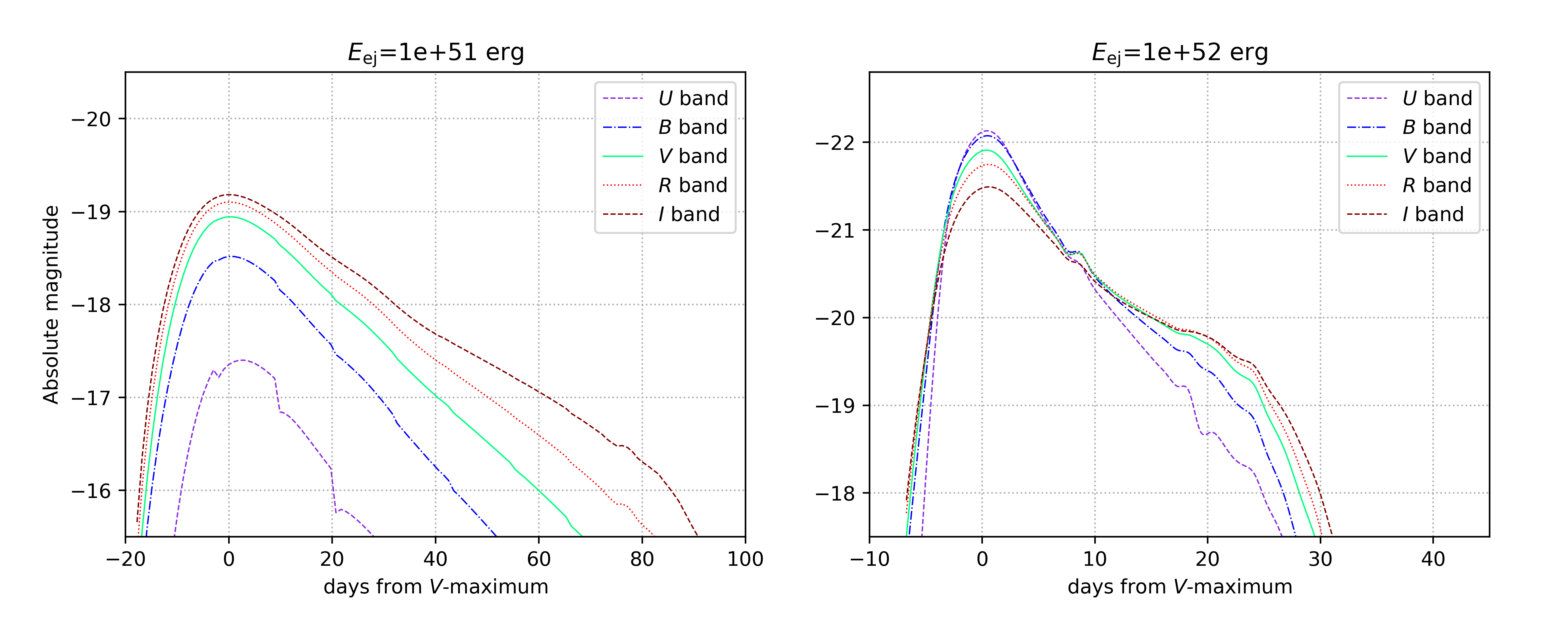
We plot in Figure 12 absolute magnitudes in $U,\,B,\,V,\,R,\,I$ bands. As seen from absolute magnitudes of the model shown in the left panel, $U>B>V\gtrsim R\gtrsim I$ at around their peaks. Since the color $V-R\sim 0.1$ around the peak, the temperature of the model is estimated to be $\sim 4,500\,{\rm K}$. Changing $E_{\mathrm{ej}}$ from $10^{51}\,{\rm erg}$ to $10^{52}\,{\rm erg}$ with fixed other parameters, multi-band LCs are plotted in the right panel. Compared to the model with lower explosion energy, the color becomes bluer (corresponding to the color temperature of $\sim 14,000\ {\rm K}$.). This is caused by the higher radiative flux than that of the lower explosion energy model.

Multi-band LC modelling can be a tool to additionally constraint the parameters jointly with the $t_{\mathrm{rise}}$–$L_{\mathrm{peak}}$ relation.

We compare CHIPS results with photometric data of SN IIn 1998S. This SN was discovered on 1998 March 2.68 UT in NGC 3877 by Z. Wan (Li et al. 1998). The nickel mass is estimated to be $0.15\pm 0.05M_{\odot}$ from the tail of the bolometric light curve (Fassia et al. 2000). The left panel of Figure 13 shows the bolometric LC of SN 1998S constructed by Fassia et al. 2000 and the CHIPS result for parameters $E_{\mathrm{ej}}=2.5\times 10^{51}\,{\rm erg},\,f_{\mathrm{inj}}=0.7,\,t_{\mathrm{inj}}=11\,{\rm yrs},\,M_{*}=20M_{\odot}$. While we can successfully reproduce the bolometric LC for the first $\sim 60$ days, the CHIPS model LC is fainter than the observed LC in the later epochs. This is because the energy input due to the radioactive decays of ⁵⁶Ni and ⁵⁶Co is not implemented in the CHIPS code (see also section V.2). The large explosion energy of $E_{\mathrm{ej}}=2.5\times 10^{51}\,{\rm erg}$, which is necessary to reproduce the observed LC, is consistent with the production of the large nickel mass of $0.15M_{\odot}$ (Hamuy 2003; Müller et al. 2017, e.g.,). The multi-band LCs obtained by Fassia et al. 2000; Liu et al. 2000 are plotted in the right panel, together with those of the same CHIPS model. As can be seen from the panel, each light curve in the early-middle epochs can be reproduced by CHIPS code as well.

In the following, we discuss the dependence of the characteristic observable quantities $L_{\mathrm{peak}},\,t_{\mathrm{rise}}$ on our results. Thanks to the enormous observations of interaction-powered transients, we know the following features:

• •

  SNe IIn: $L_{\mathrm{peak}}\sim(\mathrm{a\,few}-10)\times 10^{42}\,{\rm erg/s}$, $t_{\mathrm{rise}}\sim(1-\mathrm{a\,few})\times 10\,\mathrm{days}$ (Ofek et al. 2014b)

• •

  RETs: $L_{\mathrm{peak}}\sim(1-\mathrm{a\,few})\times 10^{43}\,{\rm erg/s}$, $t_{\mathrm{rise}}\sim(\mathrm{a\,few}-10)\,\mathrm{days}$ (Pursiainen et al. 2018)

• •

  FBOTs: $L_{\mathrm{peak}}\sim(1-\mathrm{a\,few})\times 10^{44}\,{\rm erg/s}$, $t_{\mathrm{rise}}\sim(1-\mathrm{a\,few})\,\mathrm{days}$ (Arcavi et al. 2016)

We can successfully obtain parameter spaces that are consistent the above observed regions in Figures 9, 10, and 11. The parameter spaces that give $t_{\mathrm{inj}},\,L_{\mathrm{peak}}$ of SNe IIn can be inferred as $f_{\mathrm{inj}}>0.8,\,E_{\mathrm{ej}}<10^{51}\,{\rm erg},\,t_{\mathrm{inj}}\sim 10\,{\rm yrs}$, for example. The indicated lower explosion energies are consistent with the small amount of ${}^{56}\mathrm{Ni}$ compared to that of typical SNe (Smith 2014; Elias-Rosa et al. 2018, e.g.,). $t_{\mathrm{inj}}$ has to be selected so that $t_{\mathrm{rise}}$ takes a maximum for given other parameters. Meanwhile, there is a degeneracy in parameters which give a shorter rise time and higher peak luminosity, typical observables of RETs and FBOTs. Fitting the multi-color LCs to these observed quantities may break this degeneracy, which we will explore in a forthcoming study.

References

- Arcavi et al. (2016) Arcavi, I., Wolf, W. M., Howell, D. A., et al. 2016, ApJ, 819, 35, doi: 10.3847/0004-637X/819/1/35
- Arnett (1980) Arnett, W. D. 1980, ApJ, 237, 541, doi: 10.1086/157898
- Arnett (1982) —. 1982, ApJ, 253, 785, doi: 10.1086/159681
- Asplund et al. (2009) Asplund, M., Grevesse, N., Sauval, A. J., & Scott, P. 2009, ARA&A, 47, 481, doi: 10.1146/annurev.astro.46.060407.145222
- Bessell (1990) Bessell, M. S. 1990, PASP, 102, 1181, doi: 10.1086/132749
- Castor et al. (1975) Castor, J. I., Abbott, D. C., & Klein, R. I. 1975, ApJ, 195, 157, doi: 10.1086/153315
- Chatzopoulos et al. (2012) Chatzopoulos, E., Wheeler, J. C., & Vinko, J. 2012, ApJ, 746, 121, doi: 10.1088/0004-637X/746/2/121
- Chevalier (1982) Chevalier, R. A. 1982, ApJ, 258, 790, doi: 10.1086/160126
- Chevalier & Irwin (2011) Chevalier, R. A., & Irwin, C. M. 2011, ApJ, 729, L6, doi: 10.1088/2041-8205/729/1/L6
- Chevalier & Irwin (2012) —. 2012, ApJ, 747, L17, doi: 10.1088/2041-8205/747/1/L17
- Chugai et al. (2004) Chugai, N. N., Blinnikov, S. I., Cumming, R. J., et al. 2004, MNRAS, 352, 1213, doi: 10.1111/j.1365-2966.2004.08011.x
- Das & Ray (2017) Das, S., & Ray, A. 2017, ApJ, 851, 138, doi: 10.3847/1538-4357/aa97e1
- Dessart et al. (2015) Dessart, L., Audit, E., & Hillier, D. J. 2015, MNRAS, 449, 4304, doi: 10.1093/mnras/stv609
- Dessart et al. (2010) Dessart, L., Livne, E., & Waldman, R. 2010, MNRAS, 405, 2113, doi: 10.1111/j.1365-2966.2010.16626.x
- Drout et al. (2014) Drout, M. R., Chornock, R., Soderberg, A. M., et al. 2014, ApJ, 794, 23, doi: 10.1088/0004-637X/794/1/23
- Elias-Rosa et al. (2018) Elias-Rosa, N., Van Dyk, S. D., Benetti, S., et al. 2018, ApJ, 860, 68, doi: 10.3847/1538-4357/aac510
- Fassia et al. (2000) Fassia, A., Meikle, W. P. S., Vacca, W. D., et al. 2000, MNRAS, 318, 1093, doi: 10.1046/j.1365-8711.2000.03797.x
- Fernández et al. (2018) Fernández, R., Quataert, E., Kashiyama, K., & Coughlin, E. R. 2018, MNRAS, 476, 2366, doi: 10.1093/mnras/sty306
- Ginzburg & Balberg (2012) Ginzburg, S., & Balberg, S. 2012, ApJ, 757, 178, doi: 10.1088/0004-637X/757/2/178
- Hamuy (2003) Hamuy, M. 2003, ApJ, 582, 905, doi: 10.1086/344689
- Harris et al. (2020) Harris, C. R., Millman, K. J., van der Walt, S. J., et al. 2020, Nature, 585, 357, doi: 10.1038/s41586-020-2649-2
- Ho et al. (2020) Ho, A. Y. Q., Perley, D. A., Kulkarni, S. R., et al. 2020, ApJ, 895, 49, doi: 10.3847/1538-4357/ab8bcf
- Horiuchi et al. (2011) Horiuchi, S., Beacom, J. F., Kochanek, C. S., et al. 2011, ApJ, 738, 154, doi: 10.1088/0004-637X/738/2/154
- Hunter (2007) Hunter, J. D. 2007, Computing in Science & Engineering, 9, 90, doi: 10.1109/MCSE.2007.55
- Iglesias & Rogers (1996) Iglesias, C. A., & Rogers, F. J. 1996, ApJ, 464, 943, doi: 10.1086/177381
- Ivanov & Fernández (2021) Ivanov, M., & Fernández, R. 2021, ApJ, 911, 6, doi: 10.3847/1538-4357/abe59e
- Kankare et al. (2012) Kankare, E., Ergon, M., Bufano, F., et al. 2012, MNRAS, 424, 855, doi: 10.1111/j.1365-2966.2012.21224.x
- Kashiyama & Quataert (2015) Kashiyama, K., & Quataert, E. 2015, MNRAS, 451, 2656, doi: 10.1093/mnras/stv1164
- Kiewe et al. (2012) Kiewe, M., Gal-Yam, A., Arcavi, I., et al. 2012, ApJ, 744, 10, doi: 10.1088/0004-637X/744/1/10
- Ko et al. (2021) Ko, T., Tsuna, D., Takei, Y., & Shigeyama, T. 2021, arXiv e-prints, arXiv:2112.14909. https://arxiv.org/abs/2112.14909
- Kochanek (2014) Kochanek, C. S. 2014, ApJ, 785, 28, doi: 10.1088/0004-637X/785/1/28
- Kuriyama & Shigeyama (2020) Kuriyama, N., & Shigeyama, T. 2020, A&A, 635, A127, doi: 10.1051/0004-6361/201937226
- Kuriyama & Shigeyama (2021) —. 2021, A&A, 646, A118, doi: 10.1051/0004-6361/202038637
- Kutsuna & Shigeyama (2015) Kutsuna, M., & Shigeyama, T. 2015, PASJ, 67, 54, doi: 10.1093/pasj/psv028
- Levermore & Pomraning (1981) Levermore, C. D., & Pomraning, G. C. 1981, ApJ, 248, 321, doi: 10.1086/159157
- Li & Morozova (2021) Li, C., & Morozova, V. 2021, arXiv e-prints, arXiv:2112.15181. https://arxiv.org/abs/2112.15181
- Li et al. (1998) Li, W. D., Li, C., Filippenko, A. V., & Moran, E. C. 1998, IAU Circ., 6829, 1
- Liu et al. (2000) Liu, Q. Z., Hu, J. Y., Hang, H. R., et al. 2000, A&AS, 144, 219, doi: 10.1051/aas:2000208
- Lovegrove & Woosley (2013) Lovegrove, E., & Woosley, S. E. 2013, ApJ, 769, 109, doi: 10.1088/0004-637X/769/2/109
- MacFadyen & Woosley (1999) MacFadyen, A. I., & Woosley, S. E. 1999, ApJ, 524, 262, doi: 10.1086/307790
- Magee et al. (1995) Magee, N. H., Abdallah, J., J., Clark, R. E. H., et al. 1995, in Astronomical Society of the Pacific Conference Series, Vol. 78, Astrophysical Applications of Powerful New Databases, ed. S. J. Adelman & W. L. Wiese, 51
- Matzner & McKee (1999) Matzner, C. D., & McKee, C. F. 1999, ApJ, 510, 379, doi: 10.1086/306571
- Mauerhan et al. (2013) Mauerhan, J. C., Smith, N., Silverman, J. M., et al. 2013, MNRAS, 431, 2599, doi: 10.1093/mnras/stt360
- Mauron & Josselin (2011) Mauron, N., & Josselin, E. 2011, A&A, 526, A156, doi: 10.1051/0004-6361/201013993
- Moriya et al. (2011) Moriya, T., Tominaga, N., Blinnikov, S. I., Baklanov, P. V., & Sorokina, E. I. 2011, MNRAS, 415, 199, doi: 10.1111/j.1365-2966.2011.18689.x
- Moriya (2014) Moriya, T. J. 2014, A&A, 564, A83, doi: 10.1051/0004-6361/201322992
- Moriya et al. (2013) Moriya, T. J., Maeda, K., Taddia, F., et al. 2013, MNRAS, 435, 1520, doi: 10.1093/mnras/stt1392
- Morozova et al. (2020) Morozova, V., Piro, A. L., Fuller, J., & Van Dyk, S. D. 2020, ApJ, 891, L32, doi: 10.3847/2041-8213/ab77c8
- Morozova et al. (2015) Morozova, V., Piro, A. L., Renzo, M., et al. 2015, ApJ, 814, 63, doi: 10.1088/0004-637X/814/1/63
- Morozova et al. (2017) Morozova, V., Piro, A. L., & Valenti, S. 2017, ApJ, 838, 28, doi: 10.3847/1538-4357/aa6251
- Müller et al. (2017) Müller, T., Prieto, J. L., Pejcha, O., & Clocchiatti, A. 2017, ApJ, 841, 127, doi: 10.3847/1538-4357/aa72f1
- Nadezhin (1980) Nadezhin, D. K. 1980, Ap&SS, 69, 115, doi: 10.1007/BF00638971
- Nieuwenhuijzen & de Jager (1990) Nieuwenhuijzen, H., & de Jager, C. 1990, A&A, 231, 134
- Ofek et al. (2014a) Ofek, E. O., Sullivan, M., Shaviv, N. J., et al. 2014a, ApJ, 789, 104, doi: 10.1088/0004-637X/789/2/104
- Ofek et al. (2014b) Ofek, E. O., Arcavi, I., Tal, D., et al. 2014b, ApJ, 788, 154, doi: 10.1088/0004-637X/788/2/154
- Owocki et al. (2019) Owocki, S. P., Hirai, R., Podsiadlowski, P., & Schneider, F. R. N. 2019, MNRAS, 485, 988, doi: 10.1093/mnras/stz461
- Pastorello et al. (2007) Pastorello, A., Smartt, S. J., Mattila, S., et al. 2007, Nature, 447, 829, doi: 10.1038/nature05825
- Pastorello et al. (2013) Pastorello, A., Cappellaro, E., Inserra, C., et al. 2013, ApJ, 767, 1, doi: 10.1088/0004-637X/767/1/1
- Paxton et al. (2011) Paxton, B., Bildsten, L., Dotter, A., et al. 2011, ApJS, 192, 3, doi: 10.1088/0067-0049/192/1/3
- Paxton et al. (2013) Paxton, B., Cantiello, M., Arras, P., et al. 2013, ApJS, 208, 4, doi: 10.1088/0067-0049/208/1/4
- Paxton et al. (2015) Paxton, B., Marchant, P., Schwab, J., et al. 2015, ApJS, 220, 15, doi: 10.1088/0067-0049/220/1/15
- Paxton et al. (2018) Paxton, B., Schwab, J., Bauer, E. B., et al. 2018, ApJS, 234, 34, doi: 10.3847/1538-4365/aaa5a8
- Paxton et al. (2019) Paxton, B., Smolec, R., Schwab, J., et al. 2019, ApJS, 243, 10, doi: 10.3847/1538-4365/ab2241
- Perley et al. (2019) Perley, D. A., Mazzali, P. A., Yan, L., et al. 2019, MNRAS, 484, 1031, doi: 10.1093/mnras/sty3420
- Perley et al. (2021) Perley, D. A., Ho, A. Y. Q., Yao, Y., et al. 2021, arXiv e-prints, arXiv:2103.01968. https://arxiv.org/abs/2103.01968
- Popov (1993) Popov, D. V. 1993, ApJ, 414, 712, doi: 10.1086/173117
- Prentice et al. (2018) Prentice, S. J., Maguire, K., Smartt, S. J., et al. 2018, ApJ, 865, L3, doi: 10.3847/2041-8213/aadd90
- Pursiainen et al. (2018) Pursiainen, M., Childress, M., Smith, M., et al. 2018, MNRAS, 481, 894, doi: 10.1093/mnras/sty2309
- Quataert et al. (2019) Quataert, E., Lecoanet, D., & Coughlin, E. R. 2019, MNRAS, 485, L83, doi: 10.1093/mnrasl/slz031
- Quataert & Shiode (2012) Quataert, E., & Shiode, J. 2012, MNRAS, 423, L92, doi: 10.1111/j.1745-3933.2012.01264.x
- Richardson et al. (2014) Richardson, D., Jenkins, Robert L., I., Wright, J., & Maddox, L. 2014, AJ, 147, 118, doi: 10.1088/0004-6256/147/5/118
- Savage & Mathis (1979) Savage, B. D., & Mathis, J. S. 1979, ARA&A, 17, 73, doi: 10.1146/annurev.aa.17.090179.000445
- Schlegel (1990) Schlegel, E. M. 1990, MNRAS, 244, 269
- Schneider et al. (2021) Schneider, F. R. N., Podsiadlowski, P., & Müller, B. 2021, A&A, 645, A5, doi: 10.1051/0004-6361/202039219
- Smartt et al. (2009) Smartt, S. J., Eldridge, J. J., Crockett, R. M., & Maund, J. R. 2009, MNRAS, 395, 1409, doi: 10.1111/j.1365-2966.2009.14506.x
- Smith (2014) Smith, N. 2014, ARA&A, 52, 487, doi: 10.1146/annurev-astro-081913-040025
- Smith & Arnett (2014) Smith, N., & Arnett, W. D. 2014, ApJ, 785, 82, doi: 10.1088/0004-637X/785/2/82
- Smith & McCray (2007) Smith, N., & McCray, R. 2007, ApJ, 671, L17, doi: 10.1086/524681
- Soker & Gilkis (2017) Soker, N., & Gilkis, A. 2017, MNRAS, 464, 3249, doi: 10.1093/mnras/stw2546
- Suzuki et al. (2020) Suzuki, A., Moriya, T. J., & Takiwaki, T. 2020, ApJ, 899, 56, doi: 10.3847/1538-4357/aba0ba
- Suzuki et al. (2021) Suzuki, A., Nicholl, M., Moriya, T. J., & Takiwaki, T. 2021, ApJ, 908, 99, doi: 10.3847/1538-4357/abd6ce
- Svirski et al. (2012) Svirski, G., Nakar, E., & Sari, R. 2012, ApJ, 759, 108, doi: 10.1088/0004-637X/759/2/108
- Takei & Shigeyama (2020) Takei, Y., & Shigeyama, T. 2020, PASJ, 72, 67, doi: 10.1093/pasj/psaa050
- Takei et al. (2021) Takei, Y., Tsuna, D., Kuriyama, N., Ko, T., & Shigeyama, T. 2021, CHIPS: Complete History of Interaction-Powered Supernovae, 1.0.1, Zenodo, doi: 10.5281/zenodo.6336653
- Tsuna et al. (2020) Tsuna, D., Ishii, A., Kuriyama, N., Kashiyama, K., & Shigeyama, T. 2020, ApJ, 897, L44, doi: 10.3847/2041-8213/aba0ac
- Tsuna et al. (2019) Tsuna, D., Kashiyama, K., & Shigeyama, T. 2019, ApJ, 884, 87, doi: 10.3847/1538-4357/ab40ba
- Tsuna et al. (2021a) —. 2021a, ApJ, 914, 64, doi: 10.3847/1538-4357/abfaf8
- Tsuna et al. (2021b) —. 2021b, ApJ, 922, L34, doi: 10.3847/2041-8213/ac3997
- Tsuna et al. (2021c) Tsuna, D., Takei, Y., Kuriyama, N., & Shigeyama, T. 2021c, PASJ, 73, 1128, doi: 10.1093/pasj/psab063
- van Marle et al. (2010) van Marle, A. J., Smith, N., Owocki, S. P., & van Veelen, B. 2010, MNRAS, 407, 2305, doi: 10.1111/j.1365-2966.2010.16851.x
- Vink et al. (2001) Vink, J. S., de Koter, A., & Lamers, H. J. G. L. M. 2001, A&A, 369, 574, doi: 10.1051/0004-6361:20010127
- Woosley (1993) Woosley, S. E. 1993, ApJ, 405, 273, doi: 10.1086/172359
- Woosley et al. (2007) Woosley, S. E., Blinnikov, S., & Heger, A. 2007, Nature, 450, 390, doi: 10.1038/nature06333
- Woosley & Heger (2015) Woosley, S. E., & Heger, A. 2015, ApJ, 810, 34, doi: 10.1088/0004-637X/810/1/34