Whittle Index Based Scheduling Policy for Minimizing the Cost of Age of InformationThanks: This work was funded by the Australian Research Council Discovery Project (DP180104062).Thanks: Z. Tang, N. Yang, and X. Zhou are with the School of Engineering, Australian National University, Canberra, ACT 2600, Australia (Email: {zhifeng.tang, nan.yang, xiangyun.zhou}@anu.edu.au). Z. Sun is with the School of Computer Science, Northwestern Polytechnical University, Xi’an, Shaanxi 710072, China. She was with the School of Engineering, Australian National University, Canberra, ACT 2600, Australia (Email: zsun@nwpu.edu.cn).
Abstract
We design a new scheduling policy to minimize the general non-decreasing cost function of age of information (AoI) in a multiuser system. In this system, the base station stochastically generates time-sensitive packets and transmits them to corresponding user equipments via an unreliable channel. We first formulate the transmission scheduling problem as an average cost constrained Markov decision process problem. Through introducing the service charge, we derive the closed-form expression for the Whittle index, based on which we design the scheduling policy. Using numerical results, we demonstrate the performance gain of our designed scheduling policy compared to the existing policies, such as the optimal policy, the on-demand Whittle index policy, and the age greedy policy.
Index Terms:
Age of information, Markov decision process problem, scheduling policy, Whittle index.I Introduction
Ultra-reliable and low-latency communication (URLLC) has been acknowledged as one of the enabling communication paradigms for the fifth generation (5G) networks [1]. As many real-time URLLC applications emerge [2], e.g., intelligent transportation and factory automation, the timeliness of information becomes increasingly critical. In order to fully characterize the freshness of delivered information, a new performance metric – Age of Information (AoI) – was proposed [3]. In particular, the AoI is defined as the time elapsed since the latest successfully received information was generated by the transmitter, which captures both the latency and the generation time of each information update.
Since being introduced in [3], the concept of AoI has reaped a wide range of attention. Starting from analyzing the AoI performance in [4, 5, 6, 7, 8], some transmission policies were designed to effectively improve the AoI performance [9, 10, 11, 12, 13, 14, 15, 16]. Among them, the transmission scheduling policy was optimized to minimize the average AoI for multiple-source systems in [14, 15, 16]. In particular, [14] proposed a Whittle index based scheduling policy to minimize the average AoI, where both a deterministic packet generation model and a reliable link were considered. [15] extended it to a stochastic packet generation model, while considering a system without buffer. In [16], buffers were introduced and a Whittle index based scheduling policy was designed to minimize the average AoI under an unreliable link.
In the aforementioned studies, the performance metric employed to design the scheduling policy is the average AoI. Recently, the general function of the AoI has been introduced as a natural extension to the average AoI [17, 18, 19, 20], which characterizes how the level of dissatisfaction depends on data staleness. In [17], the weighted sum of the AoI of all sources was adopted as the performance metric to optimize the scheduling policy. Then the non-linear functions of the AoI were proposed in [18, 19, 20]. In [18], the average cost of AoI was derived for three sample functions in an M/M/1 queue model with a first-come-first-served (FCFS) queue discipline. In [19], a threshold based scheduling policy was proposed to optimize a general average cost of AoI in network control systems. Considering a general non-decreasing functions of the AoI, [20] designed the Whittle index based scheduling policy. However, only the deterministic packet generation model was considered in [20], while the stochastic packet generation model remains unexplored. This motivates our work.
In this paper, we design a new scheduling policy that minimizes the general non-deceasing cost function of AoI in a multiuser system with stochastic packet arrivals and unreliable channels. Comparing with [12] and [13], we analyze the impact of stochastic packet arrivals on the scheduling policy design to minimize the general non-deceasing cost function of AoI, instead of AoI itself. In particular, we first derive the closed-form expression for Whittle index and establish the corresponding indexability. Comparing with [20], which considered deterministic packet generation, the index derivation is more challenging since we analyze the impact of the stochastic packet arrival on the scheduling policy design. By considering stochastic packet generation, the queuing delay forms the second-dimension of the system state. The one-dimensional analysis in [20] cannot be applied to the two-dimensional system. Based on the closed-form expression for Whittle index, we propose a scheduling policy to minimize the general non-deceasing cost function of AoI. Aided by numerical results, we show that our proposed policy achieves profound AoI performance improvement compared to the existing policies, for given non-decreasing functions. We also show that our proposed policy achieves a larger AoI performance gain in the heterogeneous case where user equipments (UEs) have different packet generation probabilities than the homogeneous case where UEs have the same packet generation probability.
II System Model and Problem Formulation
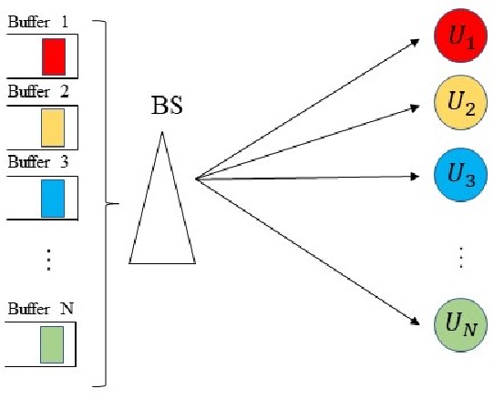
We consider a time-slotted multiuser system, as depicted in Fig. 1, where the base station (BS) transmits packets to different UEs, denoted by . We assume that there are buffers at the BS, each of which corresponds to one UE. At the beginning of each time slot, the BS generates the packet of with a probability , 11 1 We assume that the packet generation process is independent but not identical among UEs.. When the packet of is generated, it is stored in its corresponding buffer. We further assume that each buffer stores one packet such that the newly generated packet replaces the previous one in the buffer.
We assume that the BS schedules at most one packet transmission in each time slot, and hence, only the packet of one UE can be transmitted at a time. We denote a binary variable as the scheduling indicator of during time slot . If is scheduled for transmission during time slot , . Otherwise, . Thus, we obtain
| (1) |
We assume that during each time slot, packet transmission occurs prior to new packet generation. Thus, only the packets generated in previous time slots can be transmitted by the BS.
By considering practical signal propagation between the BS and UEs, the transmitted packets may not be successfully detected by UEs. We denote a binary variable as an indicator of whether or not successfully detects its packet transmitted by the BS during time slot . If the packet is successfully detected by during time slot , . Otherwise, . The transmission error probability of is denoted by , i.e., . When successfully detects a packet, it immediately sends back an acknowledgement (ACK) to the BS via an error-free control channel. The feedback overhead is assumed to be negligible as the ACK length is much smaller than the packet length. Once an ACK is received from , the BS empties the corresponding buffer by dropping the successfully received packet. Otherwise, this packet is held in the buffer.
We denote as the generation time of the last successfully detected packet at during time slot . Then, the AoI of during time slot is given by
| (2) |
Let us define as the generation time of the newest generated packet of . Until time slot , the queuing delay of this packet is computed as . The duration between the generation time of the last successfully detected packet and that of the newest generated packet is . Then, we express the AoI of as . Thus, the evolution of the AoI of is given by
| (3) |
It is noted that when the BS successfully transmits a packet to but does not generate a new packet, this successfully transmitted packet is considered as the newest generated packet. When this happens, we have and .
Based on (2), we define the average cost of AoI as
| (4) |
where is a general non-decreasing function of AoI, characterizing the importance level of packet freshness. We observe from (3) that the AoI is determined by the adopted transmission scheduling policy, i.e., . Thus, we can optimize the transmission scheduling policy to minimize the average cost of AoI in (4). The optimization problem is formulated as
| (5) |
where denotes the set of all potential transmission scheduling policies. In fact, this optimization problem is an infinite time horizon average cost constrained Markov decision process (CMDP) problem, with the state space . We note that, due to the countably infinite state space of (II), it is infeasible to obtain the optimal scheduling policy by using conventional CMDP methods, e.g., value iteration and policy iteration. To address this infeasibility, we exploit the Whittle index method to obtain a sub-optimal scheduling policy. In particular, we introduce a constant service charge as the minimum service charge of the system to schedule transmission [21]. Based on this introduction, we decouple the original CMDP problem into sub-problems with a smaller state space, where each sub-problem only involves one UE. Therefore, in order to solve the problem in (II), we optimize the average cost of AoI of each UE individually by a Lagrange function with a multiplier , given by
| (6) |
Since the AoI analysis for each UE is identical, we omit the index from , , , and in (II) to allow easy readability. Finally, to guarantee the existence of a finite average cost of AoI, we clarify that the cost function of AoI, , needs to satisfy and . Otherwise, the average cost of AoI goes to infinity.
III Index Policies
In this section, we derive the Whittle index and propose a Whittle index based scheduling policy. To derive the Whittle index, we first obtain the minimum average cost of AoI by solving (II). Here, we omit the time index and present the Bellman equation as
| (7) |
where
| (8) | ||||
| (9) |
and is the differential cost-to-go function with . We assume that given , in (7) is non-decreasing with , i.e., . Based on this, the optimal policy in (II) is proven to be threshold-based [22], denoted by . In particular, the action of state is to idle when , and to schedule when , where is the threshold and satisfies . In addition, both idle and schedule actions are equally appealing for state . Thus, the design of this threshold-based policy is equivalent to obtain the threshold . We next derive the threshold in the following Theorem.
Theorem 1
For the threshold-based policy , the threshold satisfies
| (10) |
for , and
| (11) |
for , where , , and if ; otherwise, .
Proof:
See Appendix A. ∎
Theorem 2
Considering the decoupled model, the scheduling policy in Theorem 1 is indexable.
Proof:
When , we obtain the thresholds in Theorem 1 for all as zero and hence, the idle state space is empty. When goes to infinity, the thresholds go to infinity. Hence, the idle state space is the entire space. In addition, for any cost , it is clear that any state is the idle state for if it is the idle state for . Hence, the idle state space for is a subset of the idle state space for . ∎
The Whittle index is defined as the minimum auxiliary service charge to ensure that both the action of being scheduled and the action of being idle are equally appealing for the current state [21]. In other words, the Whittle index is obtained as the minimum to obtain for the state . Based on this, we derive the Whittle index in Theorem 3.
Theorem 3
Let us consider one UE has a packet generation probability and a transmission error probability . When this UE is in the state , its Whittle index is given by
| (12) |
where is the minimum positive number satisfying
| (13) |
Proof:
See Appendix B. ∎
We remark that when considering the special case with a deterministic packet generation model, i.e., , the Whittle index in (3) coincides with the results in [20]. Furthermore, when considering the average cost of AoI being given by the average AoI, i.e., , the derived Whittle index in (3) matches the result in [16]. Therefore, the derived Whittle index in (3) is a general result for stochastic packet generation models and any cost function of AoI.
Based on the derived Whittle index in (3), we propose the optimal transmission scheduling policy that minimizes the average cost of AoI. In particular, for each time slot, the BS schedules the UE with the highest values of Whittle index for transmission. This is because that for the UE with a larger Whittle index, the transmission of its packet makes more contributions to reducing the average cost of AoI in the system.
IV Numerical Result and Discussion
In this section, we present numerical results to demonstrate the effectiveness of our proposed Whittle index based scheduling policy in Section III. For comparison, we first compare our scheduling policy with the optimal scheduling policy. We then employ the on-demand Whittle Index policy [20] and age greedy scheduling policy [16] as the benchmark policies.


In Fig. 2, we compare the proposed scheduling policy with the optimal scheduling policy for two users with an AoI violation function as the cost function such that if ; otherwise, . It turns out that the designed scheduling policy almost achieves the minimum average cost of AoI, which shows the optimality of our designed scheduling policy.
Fig. 3. plots the average cost of AoI versus the packet generation probability, , for the homogeneous case where all UEs share the same packet generation pattern and the same transmission error probability, i.e, , and for . We employ an AoI violation function as the cost function such that if ; otherwise, . We observe that for all , the designed scheduling policy achieves a lower average cost of AoI than the benchmark policies, especially for small , which shows the advantage of the designed scheduling policy over existing policies. This is due to the fact that the impact of packet freshness on the average cost of AoI increases when decreases and our proposed policy design is forward-looking instead of myopic, i.e., it evaluates the long term payoff.
Fig. 4. plots the average cost of AoI versus the packet generation probability, , for the heterogeneous case where half UEs have the same cost function such that if ; otherwise, . The other half UEs have another cost function such that if ; otherwise, . Given different cost functions among UEs, we observe that compared to the benchmark policies, our proposed policy achieves a larger AoI performance gain for the heterogeneous case than for the homogeneous case. This is due to the fact that UEs have different dissatisfaction levels of data staleness, which results in different impacts of UEs’ successful packet transmission on the reduction in the average cost of AoI. Importantly, such impacts are addressed in our proposed policy.
V Conclusion
This paper considered a multiuser system where a BS generates time-sensitive packets and transmits them to UEs under an unreliable channel. We employed the average cost of AoI as the metric to characterize the freshness of transmitted packets. By introducing a constant service charge, we derived the closed-form expression for the Whittle index. Based on this expression, we proposed a Whittle index based scheduling policy. Under this proposed scheduling policy, Whittle index reveals the value of each packet and the BS intends to send the most valuable packet to reduce the average cost of AoI. Using simulations, we showed that the performance gain of our proposed policy.
Appendix A Proof for Theorem 1
We first give the expression of as
| (14) |
Since the threshold can be obtained by computing , we derive for and , separately.
We first derive for . For the threshold-based policy with the threshold , the optimal action of state is to schedule, when . Then we define . Given , we obtain in (A).
| (15) |
Since (A) holds for any , we obtain
| (16) |
where . We find that is a valid solution to (16). Thus, we obtain for as (14).
We then derive for . For the threshold-based policy with the threshold , the optimal action of state is to idle, when . Then, we obtain as
| (17) |
for any , , and satisfying and . Expanding the last term recursively, we obtain
| (18) |
From (A), we obtain as
| (19) |
for . In addition, we observe from (A) that for any , , , and . By combining (7) with , we obtain
| (20) |
for . We clarify that both actions for the state are optimal and formulate it as
| (21) |
Based on (21), we obtain
| (22) |
Hence, we obtain as
| (23) |
Moreover, based on , we obtain
| (24) |
By substituting (24) into (A) and combining (A) with (A), we obtain the solution of for as the first and the second cases in (14). Furthermore, by combining (14) with , we express the optimal AoI, , as a function of the threshold and the service charge , given by
| (25) |
We then show that is non-decreasing with . Since are given for three cases in (14), we first prove that is non-decreasing with for these three cases separately. We note that , , and are non-decreasing functions with , since is a non-decreasing function with . Based on the expression for in (14), we obtainBased on the expression for in (14), we obtain
| (26) |
if . Differently, if and , we obtain
| (27) |
Based on (26) and (A), we have proved that is non-decreasing with for the second case, i.e., and , and the third case, i.e., , in (14), respectively. We then prove that is non-decreasing with for the first case, i.e., , in (14). Since , by substituting into (A), we obtain
| (28) |
We note that
| (29) |
Hence, we obtain
| (30) |
Based on the expression of in (14), we obtain
| (31) |
if . Hence, we have proved that is non-decreasing function with for three cases in (14).
We note that for the first case and the second case in (14) are equal to each other when , i.e.,
| (32) |
Combining (A), (31), with (A), we obtain that is non-decreasing for .
Moreover, we note that
| (33) |
and
| (34) |
when . Combining (33), (34), (26), with the fact that is non-decreasing for , we obtain that is a non-decreasing function with .
Based on the cost-to-go function obtained in (14), we next derive the threshold of the policy . Then, based on (21), we express (21) as
| (35) |
when . By substituting (25) into (A), we obtain (1). It is noted that since both and monotonically increase with , there is at most one possible number satisfying (1).
Appendix B Proof for Theorem 3
References
- [1] C. Li, N. Yang, and S. Yan, “Optimal transmission of short-packet communications in multiple-input single-output systems,” IEEE Trans. Veh. Technol., vol. 68, no. 7, pp. 7199–7203, Jul. 2019.
- [2] M. Simsek, A. Aijaz, M. Dohler, J. Sachs, and G. Fettweis, “5G-enabled tactile Internet,” IEEE J. Select. Areas Commun., vol. 34, no. 3, pp. 460–473, Mar. 2016.
- [3] S. Kaul, M. Gruteser, V. Rai, and J. Kenney, “Minimizing age of information in vehicular networks,” in Proc. IEEE Conf. Sensor Ad Hoc Commun. Netw., Salt Lake City, UT, Jun. 2011, pp. 350–358.
- [4] R. D. Yates and S. Kaul, “Real-time status updating: Multiple sources,” in Proc. IEEE Intern. Sympos. Inf. Theory, Cambridge, MA, Jul. 2012, pp. 2666–2670.
- [5] S. Kaul, R. Yates, and M. Gruteser, “Real-time status: How often should one update?” in Proc. IEEE Intern. Conf. Comput. Commun., Orlando, FL, Mar. 2012, pp. 2731–2735.
- [6] R. Wang, Y. Gu, H. Chen, Y. Li, and B. Vucetic, “On the age of information of short-packet communications with packet management,” in Proc. IEEE Global Commun. Conf., Waikoloa, HI, Dec. 2019, pp. 1–6.
- [7] H. Chen, Q. Wang, Z. Dong, and N. Zhang, “Multiuser scheduling for minimizing age of information in uplink MIMO systems,” Feb. 2020. [Online]. Available: https://arxiv.org/pdf/2002.00403.pdf
- [8] Q. Wang, H. Chen, C. Zhao, Y. Li, P. Popovski, and B. Vucetic, “Optimizing information freshness via multiuser scheduling with adaptive NOMA/OMA,” IEEE Intern. of Things J., vol. 7, no. 9, pp. 8178–8191, Sep. 2020.
- [9] Z. Jiang, B. Krishnamachari, X. Zheng, S. Zhou, and Z. Niu, “Timely status update in wireless uplinks: Analytical solutions with asymptotic optimality,” IEEE Intern. of Things J., vol. 6, no. 2, pp. 3885–3898, Apr. 2019.
- [10] Q. Wang, H. Chen, Y. Li, Z. Pang, and B. Vucetic, “Minimizing age of information for real-time monitoring in resource-constrained industrial IoT networks,” in Proc. IEEE Intern. Conf. Industr. Inform., Helsinki, Finland, Jul. 2019, pp. 1766–1771.
- [11] I. Kadota, A. Sinha, E. Uysal-Biyikoglu, R. Singh, and E. Modiano, “Scheduling policies for minimizing age of information in broadcast wireless networks,” IEEE/ACM Trans. Netw., vol. 26, no. 6, pp. 2637–2650, Oct. 2018.
- [12] H. Tang, J. Wang, L. Song, and J. Song, “Minimizing age of information with power constraints: Multi-user opportunistic scheduling in multi-state time-varying channels,” IEEE J. Select. Areas Commun., vol. 38, no. 5, pp. 854–868, May 2020.
- [13] M. A. Abd-Elmagid, H. S. Dhillon, and N. Pappas, “A reinforcement learning framework for optimizing age of information in RF-powered communication systems,” IEEE Trans. Commun., vol. 68, no. 8, pp. 4747–4760, Aug. 2020.
- [14] I. Kadota, E. Uysal-Biyikoglu, R. Singh, and E. Modiano, “Minimizing the age of information in broadcast wireless networks,” in Proc. Allerton Conf. on Commun. Control, and Comput., Monticello, IL, Sep. 2016, pp. 844–851.
- [15] Y. Hsu, “Age of information: Whittle index for scheduling stochastic arrivals,” in Proc. IEEE Intern. Sympos. Inf. Theory, Vail, CO, Jun. 2018, pp. 2634–2638.
- [16] J. Sun, Z. Jiang, S. Zhou, and Z. Niu, “Optimizing information freshness in broadcast network with unreliable links and random arrivals: An approximate index policy,” in Proc. IEEE Intern. Conf. Comput. Commun., Paris, France, May 2019, pp. 115–120.
- [17] J. Sun, Z. Jiang, B. Krishnamachari, S. Zhou, and Z. Niu, “Closed-form Whittle’s index-enabled random access for timely status update,” IEEE Trans. Commun., vol. 68, no. 3, pp. 1538–1551, Dec. 2020.
- [18] A. Kosta, N. Pappas, A. Ephremides, and V. Angelakis, “The cost of delay in status updates and their value: Non-linear ageing,” IEEE Trans. Commun., vol. 68, no. 8, pp. 4905 – 4918, Apr. 2020.
- [19] M. Klgel, M. H. Mamduhi, S. Hirche, and W. Kellerer, “AoI-penalty minimization for networked control systems with packet loss,” in Proc. IEEE Intern. Conf. Comput. Commun., Paris, France, May 2019, pp. 189–196.
- [20] V. Tripathi and E. Modiano, “A Whittle index approach to minimizing functions of age of information,” in Proc. Allerton Conf. on Commun. Control, and Comput., Monticello, IL, Sep. 2019, pp. 1160–1167.
- [21] P. Whittle, “Restless bandits: activity allocation in a changing world,” J. Appl. Probab., vol. 25, no. 1, pp. 287–298, Jan. 1988.
- [22] D. P. Bertsekas, Dynamic programming and optimal control. Belmont, MA: Athena Scientific, 2000.