Applied Regression Analysis of Correlations for Correlated Data

Correlated data arise in a variety of forms in many applied fields including epidemiology, social science, biology, public health, psychology, and economics. This paper is motivated by the insufficiency of existing approaches for analyzing two such datasets. The first, as detailed in Section 3.1, is a highly unbalanced multilevel clustered classroom dataset with within-class and within-school correlations, together with subject-related covariates such as race, gender, socioeconomic status, and more. The second, with full detail provided in Section S.4 of the Supplementary Material, comes from a longitudinal study where multiple sequential observations are collected on individuals over time, together with a collection of associated covariates. The observations in these two examples are not independent. Understanding, accounting for, modelling, and utilizing the correlations in datasets like these are fundamental for valid inference in statistical analysis. Equally importantly, there are numerous occasions where correlations can be of central scientific interest to draw insightful inferential conclusions. Regression type of models that can fully exploit covariate information for the analysis of correlations however are underdeveloped.

For analyzing clustered data, one of the most celebrated approaches is the mixed-effects model approach (Laird and Ware 1982) that incorporates random effects, typically additive to the fixed effects. As a result, the marginal variance of the response scales quadratically with the random effects; and the between-observations correlations are also implicitly determined. This intrinsic tie between the marginal variances and the correlations may restrict the capacity to adequately accommodate a broad range of correlation structures. While mixed-effects models are suitable for fitting categorical random effects such as grouping variables, they have limited ability to incorporate heterogeneity in variance caused by continuous random effects. In a great many applications, it is more reasonable to allow for the investigation of these components – mean, variance, and correlation – separately; see our informative comparisons with the mixed-effects model in a real data analysis in Section 3.1.

While the versatility of the mixed-effects model has been increasingly recognized in many applied fields, there are several challenging issues, including specifying and fitting complex correlation models, identifying the number of parameters involved, determining the degrees of freedom for various statistics, and quantifying their asymptotic distributions under the null hypothesis when the parameter lies on the boundary of its support (Müller, Scealy and Welsh 2013; Barr et al. 2013; Bates et al. 2015a, cf.). This sometimes gives rise to confusing, and even contradictory recommendations about what tests to use, and how and when, not only by applied workers but also by professional statisticians (Bolker et al. 2020; Luke 2017).

In the area of analyzing longitudinal data, numerous approaches have been developed for modeling the covariances; see the monograph Fitzmaurice et al. 2008, among the abundant literature. Related to the effort of this paper for incorporating covariates, there is a line of research on explicitly and parsimoniously modelling the covariances with an unconstrained parametrization via Cholesky-type decompositions. The recipe is to transform the restricted supports of the covariance matrices to unrestricted ones; then regression modelling approaches are exploited by utilizing the transformed parameters; see Pourahmadi 1999; Pourahmadi 2000; Pan and Mackenzie 2003; Ye and Pan 2006; Leng, Zhang and Pan 2010; Zhang and Leng 2012. For explicit regression analysis of correlations in longitudinal data, Zhang, Leng and Tang 2015 explored the use of hyperspherical coordinates to parametrize a correlation matrix via angles. Since these Cholesky-type decompositions are tied to the known ordering of the observations, they are unfortunately unsuitable for general correlated data such as clustered data where no ordering information is available. Indeed, as demonstrated in our real data example in Section S.4, missing or erroneous ordering of the longitudinal data may lead to inadequate model fitting for the approaches of this type.

Naturally, a statistician’s take on modeling the correlations is to apply a regression technique accounting for the potential contributions from covariates. However, there are several major interrelated challenges to doing so:

• 1.

  The matrix containing all the pairwise correlations is inherently positive definite and has ones on its main diagonal; thus the parameters lie in a highly constrained space;

• 2.

  The number of correlations is related to that of the observations in each subject/cluster; as a result, the correlation matrices for all the subjects/clusters have different dimensions when the data are unbalanced;

• 3.

  Correlated data are not necessarily ordered.

To meet the challenges, this paper makes a dedicated effort to propose and establish a novel, simple, flexible, unified inferential tool for applied regression modelling of correlations for general correlated data, regardless of whether they are ordered. As a regression model, our approach relates the entries in correlation matrices to any covariates via a new unrestricted parametrization of parameters and thus simultaneously addresses the three aforementioned challenges. Analogous to extending the support of the correlation coefficient from the unit interval to the whole real line, the new parametrization extends the support of a correlation matrix from a restricted space to an unrestricted one. A remarkable advantage of the new parametrization is its order-invariance: re-ordering the variables in the correlation matrix results in the same re-ordering of the components in the new parametrization. The two merits – unrestricted support and order-invariance – make the new parametrization an ideal device for modelling the correlation structures of generic correlated data.

This new framework enables unparalleled convenience in applications for correlation model building, as we establish new tools for both exploratory analysis (see the graphical tool in Section 2.3) and statistical inference. It not only provides a framework for multiple layers of random effects, similar to that of various mixed-effects models - see Section 2.2, but also offers opportunities for new discoveries, as we have demonstrated through our data examples. In Section 3.1 for analyzing the classroom data of Hill, Rowan and Ball 2005, which aims at finding factors affecting the math performance of elementary school students, our study reveals interesting new insights on the between-students correlations: there is significant evidence that the co-movement of their performances is affected by their social-economic status, besides the benchmarking scores of their earlier performances. We believe that this finding provides a new and fresh perspective on understanding the impact of different factors on the progress of students’ math performance. Apart from clustered data, our framework provides competitive, sometimes much better, performance when it comes to analyzing ordered observations, such as longitudinal data, as we have demonstrated by real data analysis and simulation studies presented in the Supplementary Material. In particular, our approach is competitive to existing regression tools using Cholesky-type decompositions when the ordering of the data is properly incorporated, while it substantially outperforms them when the ordering is not available or erroneous.

Our framework conveniently bridges clustered data analysis and the golden standard statistical inference built upon likelihood. Our approach to model correlations via an explicit regression model is rooted in the likelihood functions where the regularity conditions are easily satisfied in our setting, eliminating any ambiguity in specifying quantities such as the limiting distributions of test statistics and their degrees of freedom. For instance, the approach proposed in this paper makes the likelihood ratio test extremely easy and accessible in applications, as we have demonstrated in the real data example in Section 3.1. We remark further that although only linear models for correlations are studied in this paper, our framework allows viable extensions to generalized linear models, semi-parametric and non-parametric models. Therefore, we advocate our framework for its great flexibility and substantial potential as an applied tool.

The rest of the paper is organized as follows. Section 2 introduces the generalized z-transformation, outlines the correlation model and compares it to the mixed-effects model, presents maximum likelihood for parameter estimation, and provides the theoretical justification. We present two data analyses in Section 3 to illustrate the advantages of our framework over mixed-effects models when observations are not ordered, and over Cholesky-type decompositions when analyzing ordered data. A brief conclusion is made in Section 4. All technical details, one more real data analysis, and simulation examples are found in the Supplementary Material.

We introduce some notation first. For a symmetric matrix $\mathbf{A}\in\mathbb{R}^{m\times m}$, the operator $\operatorname{vecl}(\mathbf{A})\in\mathbb{R}^{m\times(m-1)/2}$ stacks the lower off-diagonal elements of $\mathbf{A}$ into a vector. The operator $\operatorname{diag}(\cdot)$ is used in two ways. When applied to a vector $\bm{v}=(v_{1},\ldots,v_{m})^{\prime}\in\mathbb{R}^{m}$, $\operatorname{diag}(\bm{v})$ becomes a diagonal matrix with diagonal terms being $v_{1},\ldots,v_{m}$. When applied to $\mathbf{A}$, $\operatorname{diag}(\mathbf{A})$ extracts the diagonals of $\mathbf{A}$ to return a length-$m$ vector. We use $e^{\mathbf{A}}$ to represent the matrix exponential of $\mathbf{A}$, and use $\log\mathbf{A}$ to denote the matrix logarithm of $\mathbf{A}$, assuming $\mathbf{A}$ is positive definite, defined respectively as $e^{\mathbf{A}}=\mathbf{Q}\operatorname{diag}(e^{\lambda_{1}},\ldots,e^{\lambda_{m}})\mathbf{Q}^{\prime}$ and $\log\mathbf{A}=\mathbf{Q}\operatorname{diag}(\log\lambda_{1},...,\log\lambda_{m})\mathbf{Q}^{\prime}$, where $\mathbf{A}=\mathbf{Q}\operatorname{diag}(\lambda_{1},\ldots,\lambda_{m})\mathbf{Q}^{\prime}$ is the eigen-decomposition of $\mathbf{A}$, with $\mathbf{Q}$ being an orthonormal matrix.

For a correlation $\rho\in(-1,1)$, the Fisher’s z-transformation is $z=\frac{1}{2}\log\frac{1+\rho}{1-\rho}\in\mathbb{R}$, transforming a restricted parameter to an unrestricted one. Archakov and Hansen 2021 recently discovered a matrix operation in the same spirit, transforming the restricted support of a correlation matrix to an unrestricted one. The transformation defines a mapping $f$ from a correlation matrix $\mathbf{R}\in\mathbb{R}^{m\times m}$ to an $m(m-1)/2$-dimensional vector denoted as $\bm{\gamma}$ via

Hereafter, we refer to this transformation as generalized z-transformation. It has the following remarkable properties.

• (a)

  One-to-one mapping between $\mathbf{R}$ and $\bm{\gamma}=f(\mathbf{R})$. Archakov and Hansen 2021 show that for any real symmetric matrix $\mathbf{G}\in\mathbb{R}^{m\times m}$, there exists a unique vector $\mathbf{x}^{*}\in\mathbb{R}^{m}$, such that $e^{\mathbf{G}[\mathbf{x}^{*}]}$ is a correlation matrix, where $\mathbf{G}[\mathbf{x}^{*}]$ denotes the matrix $\mathbf{G}$ with $\mathbf{x}^{*}$ replacing its diagonal. This ensures the existence and uniqueness of the inverse mapping in (1). To find $\mathbf{x}^{*}$, Archakov and Hansen 2021 show that the sequence $\mathbf{x}_{(k)}=\mathbf{x}_{(k-1)}-\log\operatorname{diag}\left(e^{\mathbf{G}[\mathbf{x}_{(k-1)}]}\right)$ converges to $\mathbf{x}^{*}$ as $k\to\infty$ with arbitrary $\mathbf{x}_{(0)}\in\mathbb{R}^{m}$.

  This suggests that to find $\mathbf{R}=f^{-1}(\bm{\gamma})$ from a $\bm{\gamma}$, whose support is contraint-free, one starts from a symmetric matrix $\mathbf{G}$ = $\operatorname{vecl}^{-1}(\bm{\gamma})$ with arbitrary diagonals. Then upon determining $\mathbf{x}^{*}$ with the above algorithm, the corresponding correlation matrix is $\mathbf{R}=e^{\mathbf{G}[\mathbf{x}^{*}]}$.

• (b)

  Order-invariance. Let $\bm{y}=(y_{1},\dots,y_{m})^{\prime}$ and $\bm{x}=(x_{1},\dots,x_{m})^{\prime}$ be random vectors such that $\bm{y}=\mathbf{P}\bm{x}$ where $\mathbf{P}$ is a permutation matrix. The correlations of these two vectors satisfy $\operatorname{corr}(\bm{y})=\mathbf{R}_{y}=\mathbf{P}\operatorname{corr}(\bm{x})\mathbf{P}^{\prime}=\mathbf{P}\mathbf{R}_{x}\mathbf{P}^{\prime}$. Hence, the correlations are order-invariant in the sense that if the $i$th and $j$th components of $\bm{y}$ are the $k$th and $l$th components of $\bm{x}$ before the permutation, then $\operatorname{corr}(y_{i},y_{j})=\operatorname{corr}(x_{k},x_{l})$. Following simple calculations, the corresponding generalized z-transformations, in their matrix forms, are also order-invariant since $\log(\mathbf{R}_{y})=\mathbf{P}\log(\mathbf{R}_{x})\mathbf{P}^{\prime}$.

We assume $n$ generic groups of dependent data, each consisting of $m_{i}$ observations for the $i$th group $(i=1,\ldots,n)$. The correlation matrix of each group is $\mathbf{R}_{i}=(\rho_{ijk})$, and its generalized z-transformation leads to $\bm{\gamma}_{i}=(\gamma_{ijk})$ $(i=1,\ldots,n;1\leq k<j\leq m_{i})$. Let $y_{ij}$ be the $j$th observation of group $i$ associated with covariate $\mathbf{x}_{ij}$; then given $\mathbf{x}_{ij}$ and $\mathbf{x}_{ik}$, ${\rho}_{ijk}=\text{corr}(y_{ij},y_{ik})$. Our proposal for the correlation model is simply

where $\bm{\alpha}$ is an unknown parameter which will be referred to as the matrix log-correlation parameter, and $\mathbf{w}_{ijk}\in{\mathbb{R}}^{d}$ are observations or constructions of covariates associated with $y_{j}$ and $y_{k}$ that used to model the correlation. For example, a reasonable choice of constructing $\mathbf{w}_{ijk}$ is to take the difference of the covariates at observations $j$ and $k$ for subject $i$. This ensures that the resulting correlation matrix is stationary if the covariate is time. For more general continuous covariates other than time, this choice is advantageous in avoiding concerns when extrapolation is needed. Our correlation model enables a highly parsimonious device – one parameter $\bm{\alpha}$ accounts for $n$ correlation matrices of arbitrary sizes for modelling general dependent data.

We would like to highlight that the linearity in (2) is inspired by and analogous to similar ideas in many widely used statistical models, most notably the generalized linear model. In the latter, it is achieved by relating the mean via a link function to a linear function of the covariates. In ours, linearity is attained via a matrix-log transformation.

Of course, the construction of $\mathbf{w}_{ijk}$ is flexible and can be tailor-made to suit practical scenarios; a few examples are provided below and more can be found in Section 3. In some of these examples, with some abuse of notations, we use the indices $i,j$ and $k$ differently from those in (2) in to highlight the structures of intended correlated data under discussion.

Example 1: The device in (2) can conveniently handle the correlation structure of temporally dependent data. For example, for modelling longitudinal data, the covariates $\mathbf{w}_{ijk}$ can be simply taken from the $j$th and $k$th measurements of the $i$th subject ($i\in\{1,\dots,n\};j,k\in\{1,\dots,m_{i}\}$) including their observed time $t_{ij}$ and $t_{ik}$ and other time-dependent variables. In this case, (2) can be applied in a similar spirit as in Pourahmadi 1999 and Zhang, Leng and Tang 2015.

Example 2: For clustered data with nested random effects, a typical mixed-effects model can be denoted as $y_{ijk}=g(\mathbf{x}_{ijk})+u_{i}+v_{ij}+\epsilon_{ijk}$, where three indices $i,j$ and $k$ are needed for the notation to maintain the usual interpretations of the indices in the context of mixed-effects models. Here $g(\mathbf{x}_{ijk})$ is the fixed effects properly specified as a function of covariates $\mathbf{x}_{ijk}$. The additive random errors are independent and satisfy $u_{i}\sim N(0,\sigma^{2}_{u})$, $v_{ij}\sim N(0,\sigma^{2}_{v})$, and $\epsilon_{ijk}\sim N(0,\sigma^{2})$. Then $\operatorname{cov}(y_{ijk},y_{ijk^{\prime}})=\sigma_{u}^{2}+\sigma_{v}^{2}$ for two observations sharing two common random effects, and $\operatorname{cov}(y_{ijk},y_{ij^{\prime}k^{\prime}})=\sigma_{u}^{2}$ for two observations sharing one common random effect. All the other cases are uncorrelated.

The correlation structure from this mixed-effects model can be modelled via the device in (2) by taking $\mathbf{w}_{ijk}=(w_{ijk,0},w_{ijk,1})^{\prime}$ where $w_{ijk,0}=1$ corresponds to the intercept coefficient, and $w_{ijk,1}=1$ if the $j$th and the $k$th observations are in the same group sharing two common random effects, and $w_{ijk,1}=0$ otherwise. By construction, $\gamma_{ijk}=\alpha_{0}+\alpha_{1}$ or $\gamma_{ijk}=\alpha_{0}$.

Example 3: As a generalization of Example 2, one may consider $v_{ij_{l}}\sim N(0,\sigma_{v_{l}}^{2}),l=1,\ldots,L$ in $y_{ij_{l}k}=g(\mathbf{x}_{ij_{l}k})+u_{i}+v_{ij_{l}}+\epsilon_{ijk}$ to allow heterogeneous random effects in $v$. Then $\operatorname{cov}(y_{ij_{l}k},y_{ij_{l}k^{\prime}})=\sigma_{u}^{2}+\sigma_{v_{l}}^{2}$ for two observations sharing two common random effects, and other covariances remain the same as in Example 2.

The correlation structure from this mixed-effects model can be modelled via the device in (2) by taking $\mathbf{w}_{ijk}=(w_{ijk,0},w_{ijk,1},\ldots,w_{ijk,L})^{\prime}$ where $w_{ijk,0}=1$ is the intercept, and $w_{ijk,l}$ is the dummy variable defined as $w_{ijk,l}=1$ if the $j$th and the $k$th observations are in the same group sharing the same $v_{ij_{l}}$ and $w_{ijk,l}=0$ otherwise.

Example 4: For multiple-level clustered data with $L+1$ levels, a linear mixed-effects model is

where additive random effects are independent, satisfying $u_{i_{0}\ldots i_{l}}\sim N(0,\sigma^{2}_{u_{l}})$ for $l=0,\ldots,L-1$. Then $\operatorname{cov}(y_{i_{0}\ldots i_{l}i_{l+1}\ldots i_{L}},y_{i_{0}\ldots i_{l}i^{\prime}_{l+1}\ldots i^{\prime}_{L}})=\sum_{i=0}^{l}\sigma_{u_{l}}^{2}$ for two observations sharing common $l+1$ levels of random effects.

Analogously, by appropriate coding in (2), one can set $\gamma_{ijk}=\sum_{i=0}^{l}\alpha_{l}$ for two observations sharing common $l+1$ levels of random effects.

Example 5: In crossed random-effects models, the units at the same level of a hierarchy are simultaneously classified by more than one factor. For example, a two-level additive variance components model can be denoted as $y_{i(jk)}=g(\mathbf{x}_{i(jk)})+u_{j}+v_{k}+\epsilon_{i(jk)}$, where additive random effects are independent and satisfy $u_{j}\sim N(0,\sigma^{2}_{u})$, $v_{k}\sim N(0,\sigma^{2}_{v})$ and $\epsilon_{i(jk)}\sim N(0,\sigma^{2})$. Then $\operatorname{cov}(y_{i(jk)},y^{\prime}_{i(jk)})=\sigma_{u}^{2}+\sigma_{v}^{2}$, $\operatorname{cov}(y_{i(jk)},y^{\prime}_{i(jk^{\prime})})=\sigma_{u}^{2}$ and $\operatorname{cov}(y_{i(jk)},y^{\prime}_{i(j^{\prime}k)})=\sigma_{v}^{2}$.

The correlation structure from this mixed-effects model can be modelled via the device in (2) by taking $\mathbf{w}_{ijk}=(w_{ijk,0},w_{ijk,1},w_{ijk,2})^{\prime}$ where $w_{ijk,0}=1$ is the intercept. The two dummy variables are defined as $w_{ijk,1}=1$ if the two individuals share the same $u$ effect and $w_{ijk,1}=0$ otherwise, and $w_{ijk,2}=1$ if the two individuals share the same $v$ effect and $w_{ijk,2}=0$ otherwise.

Examples 2-5 belong to a class of blocked correlation matrices arising from various clustered data structures. We remark that although our approach can characterize block-structured correlation matrices, the resulting models are not necessarily equivalent to the linear mixed effect models; we refer to Section 3.1 for an example. Therefore, caution should be exercised when making comparisons between the two classes of approaches, and we recommend that researchers be mindful of this distinction.

In the full generality of the proposed framework, the form of the correlation model in (2) can be of ANOVA or ANCOVA type, similar to analogous mean models, to deal with categorical and continuous variables that may influence the correlations in a unified fashion; see our real data examples in Section 3.

While categorical variables may easily be included in our correlation models, exploring and deciding possible continuous variables for the model is more challenging in applications, especially when data are highly unbalanced across groups and not ordered. Below we establish a key property – whose proof is given in the Supplementary Material – of the generalized z-transformation that facilitates a convenient descriptive tool to visually examine the relevance of a continuous variable.

Proposition 1 establishes a monotonic relationship between the correlations $\rho_{jk}$ and the corresponding $\gamma_{jk}$: each pair of them moves in the same direction, when all the other parameters are fixed. For those off-diagonal elements, the relationships between $\rho_{jk}$ and $\gamma_{lm}$ are case by case; see the examples Section S.2 of the Supplementary Material after the proof of Proposition 1. The monotonicity established in Proposition 1 is valuable to gain insight and guide exploratory analysis. However, the parameters in $\bm{\gamma}$ are only equivalent to the correlations after a non-linear matrix transformation and their analytical expressions in matrix form are not generally intuitive. Therefore, we recommend conducting numerical comparison between the original correlations and the transformed parameters based on individual settings and models when the need arises. For examples of such comparison, please refer to Section S.2 of the Supplementary Material.

To examine the relevance of some covariates $\mathbf{w}$ for modelling correlations, a straightforward approach is to plot some empirical estimate of $\bm{\gamma}$ versus those variables – an approach sharing the same spirit of the commonly used scatterplots in multiple regressions for assessing the pairwise associations between variables. However, for highly unbalanced data, obtaining an estimate of $\bm{\gamma}$ is difficult. Proposition 1 suggests the inspection of the association between some empirical estimate of $\bm{\rho}$, which is more readily available, and the covariates $\mathbf{w}$. We call a plot towards this purpose a generalized z-transformation correlogram, or GZT-correlogram hereinafter, as an analogue to the variogram in analyzing longitudinal data for examining the pattern in variances.

For balanced ordered data, empirical correlation matrices of the residuals can be computed after fitting a suitable mean model. From there the corresponding GZT-correlogram can be constructed in a straightforward manner. For handling more difficult situations including highly unbalanced data, we outline the following procedure.

• Step 1.

  Fit a suitable mean and variance model and obtain (standardized) residuals;

• Step 2.

  For a given continuous covariate, create sub-groups of the data by stratification;

• Step 3.

  Calculate the averaged pairwise correlations within each sub-group. While there are other choices that one can use for the same purpose, for this paper, we will explore the use of local-averaging after stratification.

• Step 4.

  Visually examine the pattern of the resulting correlations from Step 3 against the sub-groups obtained in Step 2.

If we see a systematic or monotonic trend in Step 4, according to Proposition 1, it will manifest itself in the relationship between $\gamma_{ijk}$ and the corresponding covariates. An example is shown in Figure 1, where plots depict decreasing patterns in the strength of correlations with two continuous variables, leading us to investigate the usefulness of these variables in modelling correlations.

Having developed a regression model for the transformed correlations, we complement it by including the following regression models of the mean and the log-variances

where $\mu_{ij}$ and $\sigma_{ij}^{2}\left(i=1,\ldots,n;j=1,\ldots,m_{i}\right)$ are respectively the conditional mean and variance for the $j$th measurement of the $i$th subject, $\mathbf{x}_{ij}$ and $\mathbf{z}_{ij}$ are $p\times 1$ and $q\times 1$ vectors of generic covariates for modelling the mean and the log-variances respectively. The specification of the three models for the mean, variance and correlation structures in (2) and (3) stipulates the number of parameters unequivocally as $p+q+d$, which can then be easily utilized to decide the degrees of freedoms for various statistics of interest. In contrast, in the mixed-effects type of models, it is not clear what one should regard as the degrees of freedom for random effects terms (Bates 2006; Baayen, Davidson and Bates 2008; Faraway 2015).

Let $\bm{\mu}_{i}=\left(\mu_{i1},\ldots,\mu_{im_{i}}\right)^{\prime},\mathbf{D}_{i}=\operatorname{diag}\left(\sigma_{i1},\ldots,\sigma_{im_{i}}\right)$ and $\bm{\omega}=\left(\bm{\beta}^{\prime},\bm{\alpha}^{\prime},\bm{\lambda}^{\prime}\right)^{\prime}$. Write $\bm{\nu}_{i}=\mathbf{y}_{i}-\bm{\mu}_{i}$ as the random error associated with the $i$th subject. Then $\bm{\Sigma}_{i}=\operatorname{cov}(\bm{\nu}_{i})=\mathbf{D}_{i}\mathbf{R}_{i}\mathbf{D}_{i}$. If $\mathbf{y}_{i}$ follows Gaussian distribution, the log-likelihood is given by

Let $\widehat{\bm{\omega}}=\left(\widehat{\bm{\beta}}^{\prime},\widehat{\bm{\alpha}}^{\prime},\widehat{\bm{\lambda}}^{\prime}\right)^{\prime}$ be the maximum likelihood estimator. An algorithm for obtaining $\widehat{\bm{\omega}}$ is provided in detail in the Supplementary Material.

In establishing the properties of $\widehat{\bm{\omega}}$, we assume the following regularity conditions.

• (A1)

  The dimensions $p,q$ and $d$ of covariates $\mathbf{x}_{ij}$, $\mathbf{z}_{ij}$ and $\mathbf{w}_{ijk}$ are fixed, and $\max_{1\leqslant i\leqslant n}m_{i}$ is bounded.

• (A2)

  The parameter space $\bm{\Omega}$ of $\left(\bm{\beta}^{\prime},\bm{\alpha}^{\prime},\bm{\lambda}^{\prime}\right)^{\prime}$ is a compact set in $\mathbb{R}^{p+d+q}$, and the true value $\bm{\omega}_{0}=\left(\bm{\beta}_{0}^{\prime},\bm{\alpha}_{0}^{\prime},\bm{\lambda}_{0}^{\prime}\right)^{\prime}$ is in the interior of $\bm{\Omega}$.

• (A3)

  As $n\rightarrow\infty,n^{-1}\mathbf{I}\left(\bm{\omega}_{0}\right)$ converges to a positive definite matrix $\mathcal{I}\left(\bm{\omega}_{0}\right)$, where $\mathbf{I}\left(\bm{\omega}_{0}\right)$ is the Fisher information matrix at $\bm{\omega}_{0}$.

Assumption (A1) is routinely made in the analysis of correlated data. Assumption (A2) is a conventional assumption for theoretical analysis of the maximum likelihood approach. Notably, given our model formulation, it is natural to assume that the true values of the parameters are not on the boundary of the parameter space. Assumption (A3) is a natural requirement for regression analysis in unbalanced longitudinal data modelling. We establish the following asymptotic results for the maximum likelihood estimator, which support statistical inference associated with the model parameters.

Here $\widehat{\bm{\beta}}$ is asymptotically independent of $\widehat{\bm{\alpha}}$ and $\widehat{\bm{\lambda}}$, because $\bm{\beta}$ concerns the mean and $\bm{\alpha}$ and $\bm{\lambda}$ are parameters of the covariances. A consistent estimator of $\mathcal{I}(\bm{\omega}_{0})$ is $\mathcal{I}(\widehat{\bm{\omega}})$ which can be used for inference. Details containing the calculations and relevant intermediate results, and an algorithm for evaluating the maximum likelihood estimator are provided in the Supplementary Material.

From Theorem 2.1 and Chernoff 1954, we establish Corollary 1, an essential result for statistical inference in applications.

Thanks to our new modelling framework, there is no ambiguity regarding the number of parameters in the model, and thus deriving the distributions of various likelihood ratio test (LRT) statistics is straightforward. We advocate the use of our approach as an appealing competitor to the mixed-effects model approach for analyzing correlated data in practice.

In this paper, we mainly illustrate our framework with a correctly specified model to avoid digression from the main message that we want to convey. If this assumption is reasonable, the maximum likelihood estimation method provides a natural approach for parameter estimation with desirable properties as we have shown. On the other hand, when this assumption is questionable, a considerable amount of research has been conducted on the properties of likelihood-based approaches, most notably along the line of the foundational work of White 1982. In Section S.5 of the Supplementary Material, we provide additional simulation studies of the impact of model misspecification. Our conclusion is that caution should be exercised in interpreting results and that there is a clear need for model diagnosis if misspecification is a concern. We recommend the use of robust alternatives when evidence of assumption violation is detected.

We analyze the classroom dataset from a study evaluating math achievement scores conducted by researchers at the University of Michigan (Hill, Rowan and Ball 2005). The primary goal of this study is to assess the improvement in math, measured by a variable called Mathgain, for kids in their early ages in relation to multiple factors. Since this is a dataset with an interesting clustering structure, elucidating the effects of the covariates on the correlation of Mathgain measures is also of great interest, not only to better model the response of interest but also for understanding the correlation pattern. In a new finding that was not revealed before, we demonstrate via our analysis some interesting co-movements of Mathgain for students with some similar conditions, which may shed light on further studies of this kind.

In this dataset, first- and third-grade students were randomly selected from classrooms in a national U.S. sample of elementary schools. Hence, there are within-class and within-school clusters, where the former are nested within the latter. After omitting items with missing values, the dataset has 1081 students from 285 classrooms in 105 schools. The number of students in each school varies from 2 to 31, making this dataset highly unbalanced. We consider Mathgain as the response variable, which measures the change in a student’s math achievement scores from the spring of kindergarten to the spring of first grade. There are eight covariates including individual-level, classroom-level, and school-level variables with a mixture of categorical and continuous ones as detailed in Table 1.

As a demonstration of linear mixed-effects models, West, Welch and Galecki 2006 recommended the following model:

where $i,j$, and $k$ index schools, classes, and individuals respectively, $s_{i}\sim N(0,\sigma_{s}^{2})$ and $c_{ij}\sim N(0,\sigma_{c}^{2})$ are independent random effects with a nested structure respectively capturing the within-school effect and within-class effect nested in schools, and $\varepsilon_{ijk}\sim N(0,\sigma^{2})$ incorporates all the remaining variations. This model serves as a benchmark in our analysis. Fitting this linear mixed-effects models via function ${\verb+lmer+}()$ in R package ${\verb+lme4+}$ gives a log-likelihood $-5160.1$ which has a Akaike information criterion (AIC) value $98.50$.

The correlations in this case are said to be blocked, a class of structures that broadly applies in analyzing clustered data. For example, if school $i$ has two classrooms with the first classroom having two observations and the second three, model (3.1) implies that

where the within-block correlation is $\rho_{1}={(\sigma_{s}^{2}+\sigma_{c}^{2})}/{(\sigma_{s}^{2}+\sigma_{c}^{2}+\sigma^{2})}$ and the between-block correlation is $\rho_{2}={\sigma_{s}^{2}}/{(\sigma_{s}^{2}+\sigma_{c}^{2}+\sigma^{2}})$.

To compare with the benchmark linear mixed-effects model in (3.1), we will take the same mean model as in (3.1), and model the log-variances as $\log\sigma^{2}=\lambda_{0}$ as in (3). For the correlation model, we set

where $i$ is the index of the schools, $j,k$ are the $j$th and $k$th individuals therein, $w_{ijk,1}=1$ if student $j$ and student $k$ come from the same classroom and $w_{ijk,1}=0$ otherwise. Thus, in our correlation model, $\alpha_{0}$ captures the between-school variability and $\alpha_{1}$ captures the additional variability between classrooms. This gives rise to the same blocked structure as in (3.1) for $\bm{\gamma}_{i}$:

and subsequently $\tilde{\mathbf{R}}_{i}=f^{-1}(\bm{\gamma}_{i})$ is also block-structured. This actually indicates that the generalized z-transformation maintains the blocked structure of the correlation matrix; see also Archakov and Hansen 2021. We note here that though model (3.1) implies a block-structured correlation matrix, $\tilde{\mathbf{R}}_{i}$ is not exactly equivalent to $\mathbf{R}_{i}$ in (3.1) for unbalanced case with unequal block sizes. Specifically, the within-block correlations of $\tilde{\mathbf{R}}_{i}$ may vary depending on the block size, whereas ${\mathbf{R}}_{i}$ assumes a common within-block correlation uniformly for all blocks as a result from the linear mixed-effect models. This is a notable consideration to keep in mind when interpreting and comparing results between the two models.

We report the results for testing the school and classroom effects for modelling correlations by applying likelihood ratio tests (LRT) for both models. As can be seen in the first three columns of Table 2, both the LRTs produce very small $p$-values for testing the school effect and the class effect within school, indicating significant statistical evidence for the school and classroom’s contribution to the correlations.

While the linear mixed-effects model (3.1) offers an effective mechanism to model classroom and school effects – the two grouping factors – as random effects, an important yet previously unaddressed question arises: are there other variables that play a role in influencing the correlations? In this application, among others of the same kind, investigating the impact of students’ math score in the spring of their kindergarten year (Mathkind) and socioeconomic status (Ses) – two continuous variables – is of particular interest. Intuitively, it would seem that students in the same class, especially those with similar math scores in their kindergarten and/or similar socioeconomic statuses, should tend to perform similarly in the future. This is simply because students with similar backgrounds may tend to undertake similar educational paths and interact more with each other. To test this out in an exploratory analysis, we obtain the residuals $\widehat{\epsilon}_{ijk}$ of each student by subtracting the fixed effects estimated from model (3.1). We standardize $\widehat{\epsilon}_{ijk}$ by dividing it by the fitted standard deviation of model (3.1), obtaining standardized residuals as $\widetilde{\epsilon}_{ijk}$. Then we calculate the empirical correlations confined to pre-defined subgroup $S$ as

where $V$ is used as a generic variable, standing for Mathkind or Ses that we are concerned about, $S$ is created by stratifying their difference, and $N_{ij}^{S}$ is the total number of different pairs in the subgroup. We examine the data by creating three subgroups – small difference: $S=(0,40]$ for Mathkind or $S=(0,0.3]$ for Ses; mid difference: $S=(40,120]$ for Mathkind or $S=(0.3,0.6]$ for Ses, and large difference: $S=(120,240]$ for Mathkind or $S=(0.6,0.9]$ for Ses. The empirical distributions of $\widehat{\rho}_{ij}^{S}$ are shown by boxplots in Figure 1, where clear decreasing trends are seen, indicating that the mathgains are indeed more correlated among students whose Mathkind or socioeconomic statuses differ relatively less.

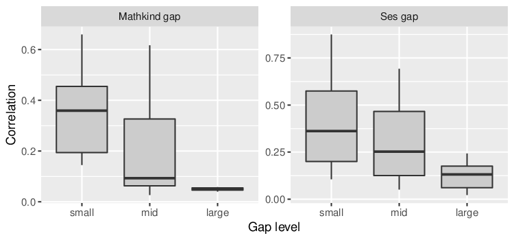
Motivated by the GZT-correlogram in Figure 1, we examine the effects of the four student-level variables for modelling correlations by expanding (11) as

In this specification, each of these variables – Sex, Minority, Mathkind, Ses – is assessed individually by varying, respectively, the definition of the dummy variable $w_{ijk,2}$ as the difference between the corresponding values of student $j$ and student $k$. We then implement the LRT for testing $H_{0}:\alpha_{2}=0$, whose $p$-values are reported in the second part of Table 2.

To make a fair comparison, we also attempt a setting for the mixed-effect models comparable to (17). Since including a continuous variable in the mixed-effects model typically means a random slope, which is different from that in (17), we do not report the results when Mathkind or Ses is included. Instead, we focus on the two categorical variables Sex and Minority by adding one more layer of random effects to (3.1) as

where the subscript $i$ indicates school, $j$ represents class, $k$ is the level of the categorical variable – Sex or Minority, and $l$ indexes the subjects in the respective group. Here the random effects are assumed independent following $s_{i}\sim N(0,\sigma^{2}_{s})$, $c_{ij}\sim N(0,\sigma^{2}_{c})$, $v_{ik}\sim N(0,\sigma^{2}_{v})$, and $\varepsilon_{ijkl}\sim N(0,\sigma^{2})$. We test the added random effect by validating $H_{0}:\sigma^{2}_{v}=0$ with the results found in Table 2.

The results in Table 2 are quite interesting. While both approaches see adding Sex as a random effect as not necessary, the linear mixed-effects model approach finds Minority marginally significant in modelling random effects, while our approach does not. We remark again from the previous discussion that for the former, testing the existence of random effects has known issues deeply rooted in the nature of such tests - the value under the null hypothesis lies on the boundary of the parameter space and thus the existing LRT is problematic. On the other hand, for our approach, the parameter value under the null in the LRT lies in the interior of its parameter space and thus our test can be easily carried out. More remarkably, this statement carries over easily to the inclusion of continuous variables in modelling correlations. As we can see from Table 2, it is found that Mathkind is a highly useful variable for depicting correlations. In contrast, the mixed-effects model does not have a natural way of incorporating continuous variables in modelling correlations, unless they are included to have random slopes, which drastically changes the question to be addressed. We further note that the student-level variables do not have to be included in a way nested in school, and the examinations in other ways are equally applicable by varying the specifications in (17) and (18). Such assessments, not reported here, do not change the conclusions on the effects of those variables.

After examining the potential impact of the variables, we conduct a model selection exercise in the context of our framework by using the Akaike information criterion (AIC): $\operatorname{AIC}=-2\widehat{l}_{\max}/n+2(p+q+d)/n,$ where $\widehat{l}_{\max}$ is the maximum of the corresponding log-likelihood. For ease in our demonstration and considering the finding from Table (2) , we narrow the full model for the correlations to:

where $w_{ijk,2}$ and $w_{ijk,3}$ are the differences between students $j$ and $k$ in their respective Mathkind and Ses variables. For the full model on the mean and log-variance as in (3), we include all the variables. The full model gives a log-likelihood $-4153.88$ and AIC value $79.50$; and the optimal model of our framework chosen by minimizing AIC gives a log-likelihood $-4156.30$ and AIC value $79.45$. These values are better than those of the benchmark model (3.1), indicating the improvement of our modelling approach due to the effective inclusion of the Mathkind or Ses as covariates for the correlations.

For completeness, we show the parameter estimates and their standard errors in Table 3. For the mean model part, all the results are similar. For the linear mixed-effects model, we are unable to report the standard errors of the random effects parameters as they are not available in the package ${\verb+lme4+}$ used in our implementation.

There are interesting results from our analysis that may be relevant in answering important questions related to assessing the improvement in math for kids in their early ages, the primary goal of this study. First, the coefficients of both Mathkind and Ses are found negative in our correlation model, which is consistent with our empirical observation from Figure 1. In particular, the negative coefficients suggest that for the kids who had similar initial performance, or similar socioeconomic backgrounds, their later math improvements tend to move in the same direction, provided that all their other conditions are controlled at the same level. Thus, these variables, especially Mathkind, may help to estimate math performance and quantify its uncertainty more faithfully to the data. Though seemingly intuitive, this finding was not discovered via other existing approaches. Moreover, there are also interesting observations from the log-variance model part. The coefficient of Mathkind is negative, suggesting that kids with higher math scores in kindergarten show lower level of variation in their later math improvement. In contrast, the coefficient of Ses is positive, implying that higher socioeconomic status score is associated with higher variance in measuring the math improvement.

We report another real data example with analyzing longitudinal data, upon applying our framework to a malaria immune response data set studied by Adjakossa et al. 2016, whose detail is provided in Section S.4 of the Supplementary Material.

First, recall that the log-likelihood is given by

Let $\bm{\Delta}_{i}=\bm{\Delta}_{i}\left(\mathbf{X}_{i}\bm{\beta}\right)=\operatorname{diag}\left\{\dot{g}^{-1}\left(\mathbf{x}_{i1}^{\prime}\bm{\beta}\right),\ldots,\dot{g}^{-1}\left(\mathbf{x}_{im_{i}}^{\prime}\bm{\beta}\right)\right\}$ where $\dot{g}^{-1}(\cdot)$ is the derivative of the inverse link function $g^{-1}(\cdot)$ and we note that $\mu(\cdot)=g^{-1}(\cdot)$. Define $\widehat{\mathbf{R}}_{i}=\mathbf{D}_{i}^{-1}\bm{\nu}_{i}\bm{\nu}_{i}^{\prime}\mathbf{D}_{i}^{-1}$, and $\mathbf{h}_{i}=\operatorname{diag}(\mathbf{R}_{i}^{-1}\widehat{\mathbf{R}}_{i})$. Then the following score equations based on the log-likelihood (20) can be obtained by direct calculation:

where $\mathbf{X}_{i},\mathbf{W}_{i}$ and $\mathbf{Z}_{i}$ are respectively the $m_{i}\times p,m_{i}(m_{i}-1)/2\times d$ and $m_{i}\times q$ matrices that contain the relevant observed covariates, and $\mathbf{1}_{m_{i}}$ is the $m_{i}\times 1$ vector with elements 1.

We define the negative expected Hessian matrix $\mathbf{I}(\bm{\omega})=-\mathbb{E}(\frac{\partial^{2}l}{\partial\bm{\omega}\partial\bm{\omega}^{\prime}})$. Following (S.1), the block expression of $\mathbf{I}(\bm{\omega})$ satisfy

where $\circ$ denotes the Hadamard product. Denote by $\bm{\eta}_{i}=\operatorname{vecl}(\mathbf{R}_{i}^{-1}\widehat{\mathbf{R}}_{i}\mathbf{R}_{i}^{-1}-\mathbf{R}_{i}^{-1})=(\eta_{ijk}),1\leq k<j\leq m_{i}$ and $\bm{\phi}_{i}=\mathbf{h}_{i}-\mathbf{1}_{m_{i}}=(\phi_{il}),1\leq l\leq m_{i}$ for $i=1,\dots,n$. Then, the $\frac{m_{i}(m_{i}-1)}{2}\times\frac{m_{i}(m_{i}-1)}{2}$ matrix $\mathbf{J}_{i}$ in $\mathbf{I}_{22}(\bm{\omega})$ and $\frac{m_{i}(m_{i}-1)}{2}\times m_{i}$ matrix $\mathbf{H}_{i}$ in $\mathbf{I}_{23}(\bm{\omega})$ can be respectively expressed as $\mathbf{J}_{i}=\mathbb{E}(\bm{\eta}_{i}\bm{\eta}_{i}^{\prime})$ and $\mathbf{H}_{i}=\mathbb{E}(\bm{\eta}_{i}\bm{\phi}_{i}^{\prime})$, since the negative expected Hessian matrix is equate to the Fisher information matrix $\mathbf{I}(\bm{\omega})=\mathbb{E}(\frac{\partial l}{\partial\bm{\omega}}\frac{\partial l}{\partial\bm{\omega}}^{\prime})$. The calculation of each element of $\mathbf{J}_{i}$ and $\bm{H}_{i}$ is given in Lemma S.1 below.

We then estimate $\bm{\omega}$ by maximizing the log-likelihood (20) via an iterative Newton-Raphson algorithm. An application of the quasi-Fisher scoring algorithm on Equation (S.1) directly yields the numerical solutions for these parameters. Since the negative expected Hessian matrix $\mathbf{I}(\bm{\omega})$ is block diagonal consisting of one block corresponding to $\bm{\beta}$ and the other to $\bm{\alpha}$ and $\bm{\lambda}$, it is natural to iterate between updating $\bm{\beta}$ and $(\bm{\alpha}^{\prime},\bm{\lambda}^{\prime})^{\prime}$. The computation needed to find the solution is summarized in Algorithm 1.

Since the likelihood function is not a global convex function of the parameters on their support, it can only be guaranteed that the algorithm converges to a local optimum. Similar to the conventional theory for the MLE, strictly speaking, the properties in Theorem 2.1 are established for the so-called consistent root of the likelihood score equation. In practice, we advocate using multiple initial values to ensure that the algorithm find an optimal solution.

To choose one reasonable initial value, we can take $\bm{\Sigma}_{i}$ as identity matrices initially and use the least-squares estimator as the initial value of $\bm{\beta}$ in the first equation of (20). Then we initiate $\bm{\alpha}$ and $\bm{\lambda}$ using the least-squares estimation based on the residuals. Our numerical experience shows that this iterative algorithm converges very quickly if we stop the iteration when $\parallel\omega^{(k+1)}-\omega^{(k)}\parallel<1e^{-7}$, usually in a few iterations. In addition, we also tried using different initial values and found that the results were not affected, unless extreme initial values that are far away from the true parameters were used.

We summarize the computation of $\mathbf{J}_{i}$ and $\bm{H}_{i}$ in the negative expected Hessian matrix in the following lemma:

References

- Adjakossa et al. (2016) [author] Adjakossa, Eric HounglaE. H., Sadissou, IbrahimI., Hounkonnou, Mahouton NorbertM. N. and Nuel, GregoryG. (2016). Multivariate longitudinal analysis with bivariate correlation test. PloS one 11 e0159649.
- Archakov and Hansen (2021) [author] Archakov, IlyaI. and Hansen, Peter ReinhardP. R. (2021). A new parametrization of correlation matrices. Econometrica 89 1699–1715.
- Baayen, Davidson and Bates (2008) [author] Baayen, R HaraldR. H., Davidson, Douglas JD. J. and Bates, Douglas MD. M. (2008). Mixed-effects modeling with crossed random effects for subjects and items. Journal of memory and language 59 390–412.
- Barr et al. (2013) [author] Barr, Dale JD. J., Levy, RogerR., Scheepers, ChristophC. and Tily, Harry JH. J. (2013). Random effects structure for confirmatory hypothesis testing: Keep it maximal. Journal of memory and language 68 255–278.
- Bates (2006) [author] Bates, DouglasD. (2006). lmer, p-values and all that.
- Bates et al. (2015a) [author] Bates, DouglasD., Kliegl, ReinholdR., Vasishth, ShravanS. and Baayen, HaraldH. (2015a). Parsimonious mixed models. arXiv preprint arXiv:1506.04967.
- Bates et al. (2015b) [author] Bates, DouglasD., Mächler, MartinM., Bolker, BenB. and Walker, SteveS. (2015b). Fitting linear mixed-effects models using lme4. Journal of Statistical Software 67 1–48.
- Bolker et al. (2020) [author] Bolker, BenB. et al. (2020). GLMM FAQ.
- Chen and Liang (2010) [author] Chen, YongY. and Liang, Kung-YeeK.-Y. (2010). On the asymptotic behaviour of the pseudolikelihood ratio test statistic with boundary problems. Biometrika 97 603–620.
- Chernoff (1954) [author] Chernoff, HermanH. (1954). On the distribution of the likelihood ratio. The Annals of Mathematical Statistics 573–578.
- Crainiceanu and Ruppert (2004) [author] Crainiceanu, Ciprian MC. M. and Ruppert, DavidD. (2004). Likelihood ratio tests in linear mixed models with one variance component. Journal of the Royal Statistical Society: Series B 66 165–185.
- Faraway (2015) [author] Faraway, Julian JJ. J. (2015). Document Accompanying “Extending the Linear Model with R”.
- Fitzmaurice et al. (2008) [author] Fitzmaurice, Garrett M.G. M., Davidian, M.M., Verbeke, G.G. and Molenberghs, G.G., eds. (2008). Longitudinal Data Analysis. Chapman & Hall/CRC.
- Hill, Rowan and Ball (2005) [author] Hill, Heather CH. C., Rowan, BrianB. and Ball, Deborah LoewenbergD. L. (2005). Effects of teachers’ mathematical knowledge for teaching on student achievement. American educational research journal 42 371–406.
- Laird and Ware (1982) [author] Laird, Nan MN. M. and Ware, James HJ. H. (1982). Random-effects models for longitudinal data. Biometrics 963–974.
- Leng, Zhang and Pan (2010) [author] Leng, ChenleiC., Zhang, WeipingW. and Pan, JianxinJ. (2010). Semiparametric mean–covariance regression analysis for longitudinal data. Journal of the American Statistical Association 105 181–193.
- Linton and McCrorie (1995) [author] Linton, OliverO. and McCrorie, J RoderickJ. R. (1995). Differentiation of an exponential matrix function. Econometric Theory 11 1182–1185.
- Luke (2017) [author] Luke, Steven GS. G. (2017). Evaluating significance in linear mixed-effects models in R. Behavior research methods 49 1494–1502.
- Mandel, Ghosh and Barnett (2022) [author] Mandel, FrancescaF., Ghosh, Riddhi PratimR. P. and Barnett, IanI. (2022). Neural networks for clustered and longitudinal data using mixed effects models. Biometrics to appear. 10.1111/biom.13615
- Müller, Scealy and Welsh (2013) [author] Müller, SamuelS., Scealy, Janice LJ. L. and Welsh, Alan HA. H. (2013). Model selection in linear mixed models. Statistical Science 28 135–167.
- Pan and Mackenzie (2003) [author] Pan, JianxinJ. and Mackenzie, GilbertG. (2003). On modelling mean-covariance structures in longitudinal studies. Biometrika 90 239–244.
- Pourahmadi (1999) [author] Pourahmadi, MohsenM. (1999). Joint mean-covariance models with applications to longitudinal data: Unconstrained parameterisation. Biometrika 86 677–690.
- Pourahmadi (2000) [author] Pourahmadi, MohsenM. (2000). Maximum likelihood estimation of generalised linear models for multivariate normal covariance matrix. Biometrika 87 425–435.
- Self and Liang (1987) [author] Self, Steven GS. G. and Liang, Kung-YeeK.-Y. (1987). Asymptotic properties of maximum likelihood estimators and likelihood ratio tests under nonstandard conditions. Journal of the American Statistical Association 82 605–610.
- West, Welch and Galecki (2006) [author] West, Brady TB. T., Welch, Kathleen BK. B. and Galecki, Andrzej TA. T. (2006). Linear Mixed Models: A Practical Guide Using Statistical Software. CRC Press.
- White (1982) [author] White, HalbertH. (1982). Maximum likelihood estimation of misspecified models. Econometrica 50 1–25. 10.2307/1912526
- Ye and Pan (2006) [author] Ye, HuajunH. and Pan, JianxinJ. (2006). Modelling covariance structures in generalized estimating equations for longitudinal data. Biometrika 93 927–941.
- Zhang and Leng (2012) [author] Zhang, WeipingW. and Leng, ChenleiC. (2012). A moving average Cholesky factor model in covariance modelling for longitudinal data. Biometrika 99 141–150.
- Zhang, Leng and Tang (2015) [author] Zhang, WeipingW., Leng, ChenleiC. and Tang, Cheng YongC. Y. (2015). A joint modelling approach for longitudinal studies. Journal of the Royal Statistical Society: Series B 77 219–238.
Supplementary Material
This Supplementary Material contains the algorithm for fitting our model, technical proofs, an application of malaria immune response data in Benin, and simulation.
S.1 The algorithm