Improving Robustness of Adversarial Attacks Using an Affine-Invariant Gradient Estimator
Abstract
As designers of artificial intelligence try to outwit hackers, both sides continue to hone in on AI’s inherent vulnerabilities. Designed and trained from certain statistical distributions of data, AI’s deep neural networks (DNNs) remain vulnerable to deceptive inputs that violate a DNN’s statistical, predictive assumptions. Before being fed into a neural network, however, most existing adversarial examples cannot maintain malicious functionality when applied to an affine transformation. For practical purposes, maintaining that malicious functionality serves as an important measure of the robustness of adversarial attacks. To help DNNs learn to defend themselves more thoroughly against attacks, we propose an affine-invariant adversarial attack, which can consistently produce more robust adversarial examples over affine transformations. For efficiency, we propose to disentangle current affine-transformation strategies from the Euclidean geometry coordinate plane with its geometric translations, rotations and dilations; we reformulate the latter two in polar coordinates. Afterwards, we construct an affine-invariant gradient estimator by convolving the gradient at the original image with derived kernels, which can be integrated with any gradient-based attack methods. Extensive experiments on ImageNet, including some experiments under physical condition, demonstrate that our method can significantly improve the affine invariance of adversarial examples and, as a byproduct, improve the transferability of adversarial examples, compared with alternative state-of-the-art methods. 11 1 The paper is under consideration at Computer Vision and Image Understanding.
1 Introduction
Deep neural networks have been widely used in image recognition [18, 33], medical image analysis [32, 25], autonomous driving [1, 17], etc. However, recent research shows that deep neural networks remain highly vulnerable to adversarial examples [36, 4, 16], since the accuracy of image recognition may degenerate significantly with the addition of small perturbations. No wonder then that more and more attention is being paid to the existence of adversarial examples that may cause safety problems.

Various adversarial attack methods have been proposed to generate robust and imperceptible adversarial examples, including the Fast Gradient Sign Method (FGSM) [16], Projected Gradient Descent (PGD) [26], and Carlini & Wagner’s method (C&W) [6], etc. However, most of these algorithms have not considered the affine transformation to the input images, which may influence the robustness of attacks [3]. As shown in Fig. 1, the resultant adversarial images generally fail to evade the classifier under affine transformation, which limits the classifier’s relevance to more practical risks. Therefore, it is imperative to generate adversarial examples that can maintain the malicious functionality required to fool the classifier under affine transformation, serving as a good measurement for the robustness of adversarial attacks.
Previous works, such as Expectation Over Transformation (EOT) [3] and Robust Physical Perturbations (RP2) [14], sample from the preset transformation distribution for estimation to make adversarial examples more robust. However, most of these works did not formally build a generic affine model, which may degrade the performance of attack methods. Besides, the sampling process adds high computational complexity, yielding low generation efficiency of adversarial examples.
1.1 Our Proposal
To address the aforementioned issues, we propose a novel method with an affine-invariant gradient estimator to generate more robust adversarial examples against a general affine transformation. Specifically, we formulate the attack problem as an optimization to maximize the expectation of adversarial loss over the affine transformation. We generate the adversarial perturbations through an ensemble of images composed of a legitimate one and its affine-transformed versions. Afterwards, we decompose the affine transformation into translation, rotation, and scaling, and derive their transformation invariance.
To improve the calculation efficiency of the gradient estimator, we derive a kernel-based estimator to approximate the affine-invariant gradient by convolving the original gradient with the specific kernels. As to the translation transformation, we implement the convolution operation referred to as the Translation-Invariant Method (TI) [10]. For rotation and scaling with higher complexity, we transfer the expectation of different rotation and scaling transformations into convolution in polar space. Theoretical analysis shows that the rotation and scaling invariance can be approximately equivalent to the translation invariance in polar space. By combining our method with any of the gradient-based attack methods (e.g., FGSM [16], PGD [26], etc.), we can obtain adversarial examples that are more robust and transferable to affine transformation, and with relatively lower computational cost.
Additionally, as an enhancement of TI [10], the proposed attack further improves the input diversity, which means better transferability for defense models according to [40, 10]. Therefore, when set as the initialization for query-based black-box attacks, the proposed method can further improve the attack success rate and reduce the required queries.
Experiments on the ImageNet dataset [30] validate the effectiveness of the proposed method. Our best method improves the attack success rate by and saves about on the computation cost, compared to EOT [3]. To verify that our method performs better when facing complex transformations in the physical world, we design physical experiments on the ImageNet classification task, and exhibit the effectiveness of our method under physical conditions. As a byproduct, we improve the transferability of the generated adversarial examples, with a higher success rate than the state-of-the-art transfer-based black-box attack against six defense models. Specifically, when set as the initialization for black-box attacks, our method can improve the attack success rate and greatly reduce the required queries by up to 95%.
In summary, we make several technical contributions:
- •
We introduce an affine-invariant attack framework to generate adversarial examples with better robustness for affine transformations, and propose a kernel-based gradient estimator to greatly improve the efficiency of our algorithm;
- •
The affine-invariant adversarial examples show great transferability for defense models and can serve as a good initialization for the black-box attacks, which improves the attack success rate and greatly reduces the queries;
- •
We design physical experiments on the Imagenet classification task, in which we print all test images and introduce transformations in the physical world, and we first statistically verified that our attacks exhibit better robustness to the complex transformations in the physical world.
The remainder of this paper is organized as follows. In Section 2, we review the background of adversarial attacks and defenses. In Section 3, we explain how the proposed affine-invariant gradient estimator works to enhance the basic attacks. In Section 4, we give a detailed analysis of gradient approximation error. Furthermore, we conduct extensive experiments and have a short discussion about the relationship between affine-invariance and transferability of adversarial examples in Section 5. Finally, we summarize the entire paper in Section 6.
2 Background
In this section, we give a detailed description of the background of adversarial attacks and defenses. Let denote the original image; denote the ground-truth label of the corresponding ; and denote an adversarial example for . A classifier can be denoted as , where is the input image, and is the class label with being the total number of classes. Our goal is to generate an adversarial example , which is not visually different from the original image , but can fool the classifier. Therefore, we often require the -norm of perturbation to be smaller than a threshold . It is expressed as , where is the budget of adversarial perturbation. With denoted as the loss function, e.g. cross entropy loss, the goal for untargeted attacks22 2 In this paper, we focus on the untargeted attacks. The attack methods can be easily extended to the targeted attacks. is to maximize the loss , which is expressed as
| (1) |
Next, we introduce some typical adversarial attacks and defenses.
2.1 White-box Attack
A white-box attack can fully access the target models. One of the most important white-box attacks is gradient-based. FGSM [16] is a common gradient-based attack algorithm, which proves that the linear features of deep neural networks in high-dimensional space are sufficient to generate adversarial examples. It performs a one-step update as
| (2) |
where is the gradient of the loss function with respect to , is the threshold of the adversarial perturbation, and is the sign function. PGD [26] extends FGSM to an iterative version. It iteratively applies gradient updates with a small step size for multiple times, and clips the adversarial examples at the end of each step as
| (3) |
where is the projection operation; is the ball centered at with radius ; and is the step size.
The optimization-based attacks aim to generate adversarial examples with minimum perturbation. Deepfool [27] is an iterative attack method based on the idea of hyper-plane classification. In each iteration, the algorithm adds a small perturbation to the image, gradually making the image cross the classification boundary, until the image is misclassified. The final perturbation is the accumulation of perturbations for each iteration. Carlini & Wagner’s method (C&W) [6] is a powerful optimization-based method. It takes a Lagrangian form and adopts Adam [22] for optimization, which is written as
| (4) |
C&W is a very effective white-box attack method, but it lacks transferability to black-box models.
2.2 Black-box Attack
Black-box attacks cannot access the parameters and gradients of the target model, and can generally be divided into transfer-based, scored-based and decision-based attacks.
Transfer-based attacks generate adversarial examples with a source model, then transfer it to the target model with the adversarial transferability [28] of the adversarial examples. MIM [9] improve the transferability by integrating a momentum term into the generation of adversarial examples. DIM [40] proposes to improve the transferability of adversarial examples by increasing the diversity of input. It applies random resizing and padding with a given probability to the inputs at each attack iteration, and feeds the outputs to the network for the gradient calculation. To further improve the transferability on some defense models, Dong et al. [10] proposed Translation-Invariant Attacks (TI). This method reduces the computational complexity by convolving untranslated gradient maps with a pre-defined kernel.
Score-based attacks can only access the output scores of the target model for each input. The attacks under this setting estimate the gradient of the target model with gradient-free methods through a set of queries. NES [20] and SPSA [38] use sampling methods to completely approximate the true gradient. Prior-guided Random Gradient-free (P-RGF) [7] improves the accuracy of estimating the gradient with a transfer-based prior. ATTACK[23] learns a probability density distribution centered around the input, and samples from the distribution to generate adversarial examples.
2.3 Defense Methods
A large variety of adversarial defense methods have been proposed to resist the increasing threat of adversarial attacks. One of the important ways is to transform the input before feeding it to the network, to reduce the influence of the adversarial perturbation; such methods include JPEG Compression [12], Bit-depth Reduction [41], and denoising methods with auto-encoder or other generative models [24, 31]. Randomization-based defenses introduce randomness to the networks to mitigate the effect of adversarial perturbation. Previous works mostly added randomness to the input [39] or the model [13]. Adversarial training [26, 37, 21, 42] is another popular defense method, which expands adversarial examples into training data to make the networks more robust against the adversarial perturbation. Certified defenses [29, 43] provide a certificate that guarantees the robustness of defense models under some threat models, and play an increasingly important role in defense methods.
3 Methodology
In this section, we give a detailed description of our proposed affine-invariant gradient estimator. In Sec. 3.1, we formulate our method as maximizing the expectation of adversarial loss for affine transformation, which is decomposed into translation and scaling-rotation transformations. In Sec. 3.2, we show how to estimate the gradient of the loss function in the convolution form. In Sec. 3.3, we formulate the solution of kernel matrices in our estimator. In Sec. 3.4, we show the attack algorithms of our method.
3.1 Problem Formulation
In order to generate more robust adversarial examples, we propose an affine-invariant attack method, which optimizes the to maximize the expectation of adversarial loss in the preset affine transformation space domain as
| (5) |
where is the random variable to affine transformation; is the probability distribution of ; and is the transformation function of , which returns the transformed image.
Considering subtle camera movement in a long distance, we can approximately decompose an affine transformation as translation, rotation, and uniform scaling transformations, while ignoring shear and flip in our method. Therefore, for any 2-D affine transformation matrix , we have:
| (6) |
where is the rotation angle; is the scaling factor; is the translation length in the x-axis, is the translation length in the y-axis; and are the random variables of the decomposed translation and scaling-rotation transformations; and and are the transformation matrices of and . According to Eq. (6), the affine transformation function should be a composition of both the translation function and the scaling-rotation function, which means:
| (7) |
where is the translation function of ; is the scaling-rotation function of ; and is the composition function of and . The decomposition process is shown in Fig. 2.

In this way, the affine transformation in the optimization problem is decomposed into two simple transformations as:
| (8) |
In order to obtain the optimal solution, we need to calculate the expectation of the gradient in Eq. (8).
3.2 Gradient Calculation
In this section, we provide a detailed calculation of the objective gradient, which is the core of gradient-based attacks. The gradient of weighted loss to the input image is expressed as:
| (9) |
where is replaced with in the final step.
In order to analyze the gradient in terms of the original images, we introduce two assumptions. The first one is that satisfies the gradient Lipschitz condition, which means smoothness of the gradient function . The second one is that the weighted sum of the distance between the transformed images and the original one is upper-bounded. With these two assumptions, we can approximate the gradient of the transformed image, by basing that approximation on the gradient of the original. We provide a detailed analysis of the gradient approximation error in Sec. 4. Accordingly, is simplified as:
| (10) |
where the approximated expectation is denoted as .
For convenience in the following steps, we assume that and are two independent random variables, which can be represented with detailed parameters and separately. Then, the gradient is expressed as:
| (11) |
where is split into , and is split into . In the final equation, we denote as , and the two expectations functions as and .
In actual implementation, sampling a series of transformed images for gradient calculation is a feasible but inefficient method [3]. In our method, we discretize the four random variables to simplify the calculation of Eq. (11). The overall framework of affine transformation decomposition and equivalence of the decomposed transformations is shown in Fig. 2. In the following part, we provide the equivalent convolution forms.
3.2.1 Equivalence of Translation
Since images are discrete 2D grids, to simplify the calculation we discretize the translation into pixel-wise shifts. Furthermore, we can set the value of and to be the moving step size in basic directions. Referring to [10], the translation part can be equivalent to convolving the gradient with a kernel composed of all weights as:
| (12) |
where and also represent the shifting step size in two basic directions; is the probability function of the translation transformation; and is the equivalent translation kernel matrix. Taking a finite number of translation transformations, i.e., and , the size of is , with .
3.2.2 Equivalence of Rotation and Scaling
For rotation and scaling, normal convolution operation does not work to simplify the calculations. However, scaling can be linearized and approximated as radial shifts in polar space, when it comes to subtle transformation. We can project the original gradient image into polar space, as shown in Fig. 2. Then, rotation and scaling can be approximated as translation in the polar space. We replace the scaling factor with a radial shift distance , such that is expressed as:
| (13) |
where and are the polar transformation and inverse polar transformation, while and are the corresponding random variables in polar space. Similarly, by discretizing the translation in polar space into pixel-wise shifts, we can get:
| (14) |
where is the translation kernel matrix of size in polar space.
Finally, the total gradient calculation is equivalent to some simple operations such that:
| (15) |
where is first convolved with a translation kernel , then convolved with another translation kernel in polar space.
3.3 Kernel Matrix
For the translation part, we set the translation step size in a limited range, with and . To ensure the attack performance on the untransformed images, we follow the basic principle that the more the input image changes, the lower the weight that should be assigned. Therefore, we empirically set matrix to follow Gaussian distribution, i.e. , where and . To ensure that the convolved gradients are at the same level as the original ones, we need to set as a normalized matrix:
| (16) |
As for the rotation and scaling parts, we can define the kernel matrix directly in polar space just as with the translation part. Following the same principle, we set , where , and , . Then the kernel is defined as:
| (17) |
The normalized convolution kernels in Eq. (16) and in Eq. (17) are used to enhance the affine invariance of the gradient map.
3.4 Attack Algorithms
In Sec. 3.2 and Sec. 3.3, we show how to calculate the gradient and corresponding kernel matrix. Here, we introduce the updating strategy of our attack method for generating adversarial examples. Essentially, our method is also related to the gradient, so it can be easily integrated into other gradient-based attack methods introduced in Sec. 2, such as FGSM [16], PGD [26], etc. For gradient-based attack methods such as PGD, we need to calculate the gradient of the current solution in each step. In our method, however, we just need to replace the normal gradient with the result of obtained by our proposed affine-invariant gradient estimator in Sec. 3.2.
For example, when combined with one-step methods such as FGSM [16] (AI-FGSM), the updating strategy is written as:
| (18) |
When combined with the iterative methods such as PGD [26] (AI-PGD), the updating strategy is written as:
| (19) |
The detailed algorithm of AI-PGD is summarized in Algorithm 1. Our method can be similarly integrated into other gradient-based attack methods such as MIM [9] and DIM [40] as AI-MIM and AI-DIM.
4 Analysis of Gradient Approximation Error
In Sec. 3.2, we introduce a gradient approximation to simplify the gradient calculation in Eq. (10) as:
| (20) |
In this section, we give a detailed analysis of the gradient approximation error to show the rationality of using gradient approximation in our method.
We let and for convenience. Furthermore, we introduce the two main assumptions used in our analysis.
DNNs introduce ReLU activation function into the structure, so the loss function of the neural networks does not satisfy the Lipschitz condition. However, recent studies [2, 15] have shown that the optimization landscape is almost-convex and semi-smooth with over-parameterized neural networks, showing the semi-smoothness of the loss function. Therefore, we can strengthen this conclusion into the first assumption.
Assumption 1.
The loss function satisfies the gradient Lipschitz condition , which means smoothness of the gradient function . A subtle affine transformation will not affect its smoothness, which is expressed as:
| (21) | |||
where is a positive constant.
For natural images, the values of two adjacent pixels are usually continuous and gradual. Therefore, when the affine transformation we perform on the image is smaller, the Euclidean distance between the transformed image and the original image is also smaller. Now we can lay out our second assumption.
Assumption 2.
The expectation of the distance between the affine transformed image and the original one is upper-bounded as:
| (22) |
where is a positive constant.
With the two assumptions, we can get Corollary 1 that the Euclidean distance between and is upper-bounded. The detailed proof is shown in Appendix A.
Corollary 1.
The Euclidean distance between and is upper-bounded as:
| (23) |
Now we get an upper bound of the approximation error. Since the gradients used for adversarial example generation in Sec. 3 would be normalized, we also care about the directions between and except distance. Then we analyze the cosine similarity between them with another assumption.
Assumption 3.
The norms of and are larger than a positive constant as
| (24) |
Assumption 3 can be satisfied when the model does not cause gradient vanishing, otherwise the adversarial examples cannot be generated since the gradients are zero. We then can analyze the difference of directions between and by their cosine similarity. We finally give the following corollary. The detailed proof is shown in Appendix A.
Corollary 2.
The cosine similarity of and is lower-bounded as:
| (25) |
where is the cosine similarity function.
In our method, we use Gaussian kernels, which can cause a relatively small . With Corollary 1 and Corollary 2, we can approximate the gradient calculation as Eq. (20) with a small approximation error.
| Method | |||||||||||||||
| Inc-v3 | Inc-v4 | Ens-AT | Inc-v3 | Inc-v4 | Ens-AT | Inc-v3 | Inc-v4 | Ens-AT | Inc-v3 | Inc-v4 | Ens-AT | Inc-v3 | Inc-v4 | Ens-AT | |
| FGSM | 72.6 | 65.8 | 38.6 | 71.3 | 57.3 | 34.7 | 79.9 | 35.6 | 12.1 | 70.0 | 57.2 | 34.9 | 71.3 | 65.7 | 42.0 |
| AI-FGSM | 83.0 | 81.0 | 73.1 | 78.0 | 73.4 | 59.7 | 63.2 | 44.0 | 23.6 | 77.5 | 72.9 | 58.9 | 79.9 | 80.7 | 63.9 |
| PGD | 60.0 | 37.1 | 20.4 | 75.2 | 30.8 | 14.2 | 100 | 24.8 | 6.3 | 73.1 | 31.5 | 15.0 | 56.8 | 36.8 | 17.6 |
| AI-PGD | 85.2 | 76.3 | 58.1 | 90.3 | 66.3 | 49.0 | 100 | 40.9 | 18.9 | 88.7 | 66.8 | 49.9 | 84.6 | 74.3 | 54.6 |
| MIM | 84.2 | 69.8 | 48.2 | 92.4 | 63.7 | 36.7 | 100 | 50.5 | 16.3 | 91.1 | 65.4 | 38.0 | 83.1 | 69.4 | 43.1 |
| AI-MIM | 92.4 | 85.8 | 70.5 | 96.0 | 82.4 | 64.3 | 100 | 59.0 | 33.3 | 95.7 | 80.8 | 65.0 | 90.6 | 86.6 | 70.8 |
| DIM | 94.9 | 82.8 | 50.3 | 97.3 | 79.6 | 46.0 | 100 | 75.4 | 21.8 | 97.7 | 78.8 | 46.8 | 94.6 | 83.1 | 47.5 |
| AI-DIM | 94.9 | 88.8 | 76.9 | 97.5 | 86.0 | 71.8 | 99.9 | 72.6 | 39.2 | 98.0 | 86.7 | 70.2 | 95.3 | 90.6 | 74.6 |
| EOT | 82.1 | 52.0 | 10.6 | 82.2 | 50.7 | 9.1 | 82.3 | 50.3 | 10.2 | 82.5 | 51.4 | 10.3 | 82.4 | 51.6 | 9.6 |
| Method | |||||||||||||||
| Inc-v3 | Inc-v4 | Ens-AT | Inc-v3 | Inc-v4 | Ens-AT | Inc-v3 | Inc-v4 | Ens-AT | Inc-v3 | Inc-v4 | Ens-AT | Inc-v3 | Inc-v4 | Ens-AT | |
| FGSM | 72.0 | 66.4 | 55.2 | 75.4 | 70.9 | 43.1 | 71.7 | 66.3 | 45.8 | 59.8 | 51.6 | 37.9 | 56.3 | 51.7 | 41.5 |
| AI-FGSM | 87.3 | 87.7 | 64.2 | 87.0 | 87.6 | 63.6 | 81.0 | 80.6 | 65.9 | 69.2 | 68.9 | 56.1 | 64.6 | 59.3 | 52.7 |
| PGD | 38.7 | 28.1 | 26.9 | 44.0 | 34.3 | 22.4 | 58.4 | 36.7 | 26.4 | 50.6 | 31.1 | 20.7 | 41.7 | 26.5 | 23.1 |
| AI-PGD | 82.0 | 83.4 | 62.7 | 85.8 | 82.9 | 58.8 | 85.1 | 73.6 | 57.1 | 73.6 | 59.6 | 48.1 | 61.5 | 51.6 | 44.2 |
| MIM | 66.0 | 60.0 | 44.8 | 75.6 | 72.0 | 40.3 | 83.5 | 69.4 | 46.8 | 74.3 | 59.8 | 42.6 | 67.9 | 56.9 | 44.6 |
| AI-MIM | 86.7 | 90.2 | 67.2 | 91.7 | 91.2 | 68.7 | 90.7 | 86.3 | 72.1 | 83.4 | 75.5 | 64.7 | 75.7 | 68.4 | 61.1 |
| DIM | 70.7 | 64.7 | 44.8 | 83.2 | 78.1 | 44.1 | 94.7 | 82.9 | 51.2 | 92.1 | 76.6 | 54.4 | 85.5 | 70.3 | 57.7 |
| AI-DIM | 90.0 | 91.1 | 67.2 | 93.0 | 93.1 | 70.9 | 95.6 | 90.7 | 75.2 | 90.6 | 82.6 | 71.3 | 85.5 | 77.9 | 69.1 |
| EOT | 52.6 | 36.2 | 16.8 | 74.6 | 47.0 | 14.4 | 82.4 | 51.6 | 9.6 | 83.6 | 62.1 | 24.9 | 81.9 | 61.4 | 30.9 |
5 Experiments
In this section, we introduce our experiments and prove the effectiveness of our method. In Sec. 5.1, we introduce the experimental settings. We then test the affine invariance and efficiency of our methods compared to some basic attacks and EOT[3] in Sec. 5.2. In Sec. 5.3, we further verify the robustness of our method to more complex transformations in the physical world. In Sec. 5.4, we verify the robustness of our methods to defense models under black-box settings. Next, we provide an ablation study for our methods in Sec. 5.5. Finally, we include a short discussion about the affine-invariance and transferability of adversarial examples in Sec. 5.6.
5.1 Experimental Settings
We first design experiments to show the improvement of our proposed attacks on affine invariance in the digital world, and then further introduce physical conditions to verify the robustness of our method to affine transformations. Finally, we demonstrate that our approach can also improve the transferability of adversarial attacks to defense models. Below are some details of the experimental setup.
Dataset and Models. We use an ImageNet-compatible dataset33 3 https://github.com/cleverhans-lab/cleverhans/tree/master/cleverhans_v3.1.0/examples/nips17_adversarial_competition/dataset comprised of the 1,000 images that were used in the NeurIPS 2017 adversarial competition. For models, we choose four naturally trained models and six defense models according to the RealSafe platform [8]. These models are naturally trained Inception v3 (Inc-v3) [35]; Inception v4 (Inc-v4) [34]; Inception ResNet v2 (IncRes-v2) [34] and ResNet v2-152 (Res-v2-152) [19]; Ensemble Adversarial Training (Ens-AT) [37]; Adversarial Logit Pairing (ALP) [21]; JPEG Compression [12]; Bit-depth Reduction (Bit-Red) [41]; Random Resizing and Padding (R&P) [39]; and RandMix [43]. Furthermore, we use Inc-v3 as the backbone model for defenses based on input transformations such as JPEG and Bit-Red.
Evaluation Metrics. We use the attack success rate as the evaluation metrics referring to RealSafe [8]. The attack success rate of an untargeted attack on the classifier is defined as:
| (26) |
where is the test set; ; is the indicator function; means the attack method that generates the adversarial examples with perturbation budget under the norm; and .
Hyper-parameters. We set the maximum perturbation to be with pixel value . For all iterative methods, we set the number of iteration steps to be . For methods with momentum, we use the decay factor . For methods related to DIM [40], we set the transformation probability as . For EOT [3], the number of samples and optimization steps are both set to be 50. In order to avoid influencing the performance of the attacks on untransformed images, we only consider affine transformations within a narrow range, with the settings , , . Also, we set the kernel size of , to and .

5.2 Robustness to Affine Transformation
In this section, we show the experimental results of the proposed affine-invariant method over different affine transformations. We selected FGSM, PGD, MIM and DIM as the basic attacks, and their extensions combined with our method are named with an ”AI-” prefix. EOT is also considered as a baseline of transform-based attacks. We choose Inc-v3 as the white-box model, and test the performance on Inc-v3 (white-box model), Inc-v4 (black-box model) and Ens-AT (defense model), respectively. We separately study the ASRs in three kinds of transformations: rotation, scaling and translation.
| Method | ||||||
| Inc-v3 | Inc-v4 | Ens-AT | Inc-v3 | Inc-v4 | Ens-AT | |
| FGSM | 76.1 | 71.1 | 45.1 | 76.7 | 70.9 | 45.0 |
| AI-FGSM | 87.0 | 87.8 | 66.0 | 88.1 | 87.4 | 69.6 |
| PGD | 43.8 | 32.8 | 17.1 | 46.6 | 33.7 | 21.4 |
| AI-PGD | 85.5 | 84.7 | 61.0 | 83.2 | 84.6 | 65.8 |
| MIM | 76.6 | 72.0 | 38.7 | 79.3 | 71.8 | 41.9 |
| AI-MIM | 91.6 | 90.7 | 73.3 | 91.7 | 90.5 | 70.9 |
| DIM | 85.2 | 78.1 | 43.2 | 85.5 | 76.8 | 44.4 |
| AI-DIM | 94.1 | 92.4 | 73.7 | 93.5 | 92.2 | 74.4 |
| EOT | 74.3 | 50.9 | 14.6 | 73.4 | 51.2 | 16.9 |
| Method | Avg ASRs(%) | Avg Time(s) | ||
|---|---|---|---|---|
| Inc-v3 | Inc-v4 | Ens-AT | ||
| EOT | 77.9 | 51.4 | 14.8 | 56580 |
| AI-DIM | 94.0 | 87.1 | 69.5 | 566 |
5.2.1 Rotation
As to rotation, we set and the rotation angle to be at a step of to see the performance of different methods under different angles. We report the test results in Tab. 1. In total, the ASRs increase significantly with the proposed method added to the basic models. Results on black-box models and defense models also demonstrate that our method is more transferable and resistant to defenses. In particular, our method brings the greatest improvement to PGD, which increases the ASR by on average. Furthermore, our best attack AI-DIM outperforms the EOT by a large margin, especially for black-box and defense models. For example, it improves the ASR by for the defense model compared to EOT. The results confirm the effectiveness of the specifically designed rotation-invariant kernel.

5.2.2 Scaling
As to scaling, we perform a stress test to verify the stability of our method. We set the rotation angle and translation offsets in an extreme condition as , , , and set the scaling factor as to show the performance under different scales. From the results in Tab. 2, we observe that our method still maintains better affine invariance under an extreme affine transformation, showing huge performance gains compared with the basic attacks and EOT. Taking in white-box attacks as an example, our method improves the ASRs by , , and for FGSM, PGD, MIM and DIM, respectively, and the best attack AI-DIM brings a performance gain compared to EOT. This demonstrates that our method improves the robustness to large-scale affine transformations. The results also prove that the kernel we designed in the polar space is effective for achieving scaling invariance.
5.2.3 Translation
As to translation, we randomly set the rotation angle and scaling factor as , . Due to the symmetry of translation, the translation offsets are set to positive numbers as . From the results in Tab. 3, we find that different translation offsets have little effect on the attack performance. Nevertheless, our method still performs better than the basic attacks and EOT, demonstrating that the translation kernel we construct referring to [10] also yields a good estimation of the gradient.
In summary, our best attack, AI-DIM, achieves an average ASR of against the white-box model, against the black-box model and against the defense model over the tested affine transformation domain. In order to further show the margin improved by our method, taking AI-DIM as the examples, we visualize the white-box attack-success-rate function with rotation angle and scaling factor as independent variables in Fig. 3. More results can be found in Appendix B. We set the translation offsets both as 0, since they have little effect on the performance. Fig. 3 show that our method keeps a relatively high attack success rate even under extreme affine transformations, showing better affine invariance than the basic attacks. In addition, we compare the efficiency of our method with EOT in Tab. 4. The experiment is conducted on a GTX 1080TI GPU. From the results, we conclude that our best method improves the attack success rate by and saves about on computation cost, compared to EOT.
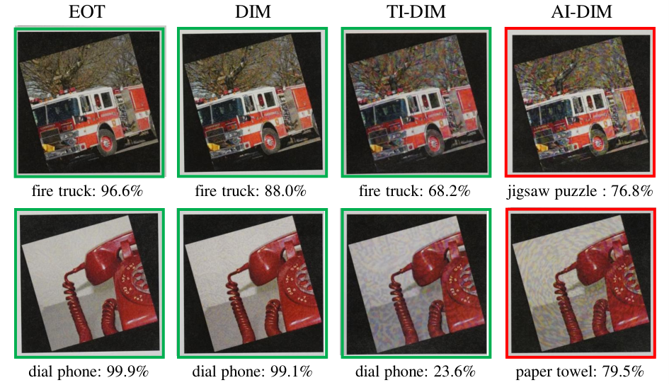
We also visualize adversarial images generated for the Inc-v3 model by DIM, and AI-DIM with different transformations in Fig. 4, respectively. More adversarial images generated by FGSM, PGD, MIM and their corresponding combinations with our method are shown in Appendix C. Due to transformation to polar space, we can see that the adversarial perturbations generated by our affine-invariant attacks exhibit circular patterns. Furthermore, the adversarial perturbations generated by our affine-invariant attacks are smoother than those generated by DIM, due to the smooth effect of kernel convolution. We further show the predicted labels and probabilities for the images with different affine transformations, and the results show that the adversarial examples generated by our method are more robust to affine transformations.
5.3 Robustness under Physical Condition
| Method | setting 1 | setting 2 | setting 3 |
|---|---|---|---|
| EOT | 24.3 | 21.6 | 18.0 |
| DIM | 11.8 | 12.7 | 15.3 |
| TI-DIM | 10.7 | 8.5 | 7.6 |
| AI-DIM | 10.5 | 5.5 | 5.6 |
| Method | Single-model attacks | Ensemble-based attacks | ||||||||||
| Ens-AT | ALP | JPEG | Bit-Red | R&P | RandMix | Ens-AT | ALP | JPEG | Bit-Red | R&P | RandMix | |
| FGSM | 16.1 | 6.4 | 37.6 | 30.0 | 48.7 | 35.0 | 27.1 | 11.1 | 49.1 | 41.8 | 58.7 | 40.7 |
| TI-FGSM | 26.1 | 21.6 | 46.9 | 40.7 | 56.5 | 42.2 | 34.2 | 22.8 | 53.9 | 47.4 | 60.2 | 44.8 |
| AI-FGSM | 31.7 | 30.7 | 48.6 | 43.8 | 57.2 | 42.0 | 34.9 | 31.7 | 49.8 | 47.8 | 59.4 | 40.2 |
| PGD | 8.4 | 0.4 | 26.7 | 19.4 | 36.6 | 12.7 | 25.8 | 0.4 | 58.0 | 32.8 | 66.8 | 23.7 |
| TI-PGD | 18.8 | 9.7 | 29.3 | 19.9 | 36.2 | 18.5 | 41.4 | 10.1 | 56.0 | 31.9 | 59.4 | 23.2 |
| AI-PGD | 31.2 | 21.8 | 48.0 | 40.4 | 57.4 | 35.2 | 54.6 | 27.6 | 72.9 | 53.2 | 75.8 | 41.5 |
| MIM | 34.5 | 5.1 | 60.3 | 44.6 | 68.6 | 40.2 | 59.1 | 10.3 | 80.6 | 62.8 | 83.4 | 51.8 |
| TI-MIM | 46.7 | 33.7 | 56.9 | 45.5 | 61.6 | 38.0 | 65.3 | 35.2 | 73.6 | 56.1 | 76.4 | 42.7 |
| AI-MIM | 49.4 | 31.9 | 65.8 | 52.0 | 70.1 | 48.5 | 69.6 | 33.7 | 81.4 | 63.9 | 84.9 | 54.3 |
| DIM | 54.7 | 8.6 | 71.3 | 58.1 | 77.1 | 50.0 | 80.2 | 14.2 | 83.4 | 69.8 | 83.8 | 52.5 |
| TI-DIM | 60.9 | 35.0 | 70.1 | 53.3 | 72.9 | 43.2 | 78.0 | 39.9 | 84.5 | 65.8 | 85.8 | 51.3 |
| AI-DIM | 62.7 | 36.4 | 76.2 | 59.8 | 78.8 | 50.0 | 82.1 | 42.6 | 89.1 | 72.2 | 90.7 | 60.7 |
| Method | Ens-AT | ALP | JPEG | Bit-Red | RP | RandMix | ||||||
|---|---|---|---|---|---|---|---|---|---|---|---|---|
| ASR | Avg Q | ASR | Avg Q | ASR | Avg Q | ASR | Avg Q | ASR | Avg Q | ASR | Avg Q | |
| NES | 95.7 | 1827 | 82.7 | 1425 | 55.8 | 6126 | 96.8 | 1132 | 8.4 | 4236 | 1.5 | 3684 |
| NES-PGD | 97.3 | 1045 | 82.3 | 1377 | 90.9 | 1688 | 98.5 | 443 | 65.2 | 895 | 47.0 | 2658 |
| NES-TI-DIM | 98.9 | 315 | 88.1 | 939 | 95.5 | 670 | 99.2 | 242 | 86.2 | 499 | 52.0 | 1524 |
| NES-AI-DIM | 99.4 | 183 | 88.5 | 937 | 97.1 | 423 | 99.7 | 154 | 91.7 | 246 | 60.7 | 1069 |
| SPSA | 96.9 | 1516 | 80.5 | 1556 | 52.0 | 6001 | 96.8 | 994 | 8.8 | 3735 | 0.7 | 3682 |
| SPSA-PGD | 97.8 | 910 | 81.9 | 1441 | 87.5 | 1753 | 98.6 | 414 | 68.6 | 863 | 25.2 | 2690 |
| SPSA-TI-DIM | 99.3 | 265 | 88.1 | 1013 | 95.5 | 637 | 99.2 | 222 | 86.0 | 476 | 51.2 | 1557 |
| SPSA-AI-DIM | 99.6 | 167 | 88.7 | 1006 | 96.6 | 410 | 99.7 | 140 | 90.5 | 223 | 61.3 | 1083 |
| ATTACK | 99.1 | 805 | 98.6 | 505 | 97.5 | 1057 | 99.6 | 577 | 31.9 | 1529 | 7.8 | 2487 |
| ATTACK-PGD | 99.7 | 395 | 98.8 | 450 | 97.8 | 244 | 99.7 | 274 | 73.6 | 340 | 27.0 | 1699 |
| ATTACK-TI-DIM | 99.8 | 147 | 99.0 | 250 | 99.3 | 126 | 99.5 | 152 | 89.2 | 271 | 53.8 | 1176 |
| ATTACK-AI-DIM | 99.9 | 87 | 98.8 | 277 | 99.7 | 58 | 99.9 | 97 | 93.0 | 131 | 63.0 | 838 |
To further exhibit the performance of our method under physical experiment condition, we print all the 1,000 adversarial images and obtain the affine-transformed test data by adjusting the camera position parameters etc. With the disturbance of physical conditions such as lighting, the classifier’s recognition accuracy for recaptured images will decrease a lot. Therefore, in this part, we will narrow down the transformation ranges such as limiting rotations within 15 degrees. We show the classifier’s recognition accuracy with different attack methods and three transformation settings in Tab. 5, which are denoted as setting 1: , setting 2: and setting 3: . Here we use the recognition accuracy as the performance indicator since in ASR will be further affected under physical condition, and recognition accuracy is more objective. Due to the inevitable deviations in the shooting process, there will be some random offsets in each transformations, such as translation offset from 0 to 20 pixels. In Fig. 5, we visualize some re-captured adversarial examples by camera for setting 3. The attack hyper-parameters are the same as the previous ones, and the source model and test model are both Inc-v3. Tab. 5 shows that even under physical condition, our method outperforms the rest three attacks, which further verifies the robustness of the proposed affine-invariant attacks to affine transformations.
5.4 Robustness to Defense Models under Black-box Setting
TI [10] has shown that it can improve the transferability of adversarial examples greatly with respect to the defense models. As shown in Sec. 3, the proposed affine-invariant method is an enhancement of the TI method. Therefore, we conduct an experiment to show the transferability of adversarial examples generated by different attacks against defense models. We test the performance of single-model attacks and ensemble-based attacks [9], respectively. For single-model attacks, we set IncRes-v2 as the surrogate model to generate adversarial examples. As for ensemble-based attacks, we attack the ensemble of Inc-v4, IncRes-v2, and Res-v2-152 with equal ensemble weights. Furthermore, we choose six state-of-the-art defense models according to RealSafe [8].
From Tab. 6, we can see that, compared with the TI method and basic attacks, our method yields a significant improvement for tested defense models. In particular, combined with PGD, MIM and DIM, our method improves the ASRs by , , and , respectively, on average for ensemble-based attacks, compared to the TI method. It demonstrates that the proposed affine-invariant attacks can better improve the tranferability of the generated adversarial examples to evade the defense models. The primary reason is that our method considers a wider transformation domain, and can generate adversarial examples that are less sensitive to the discriminative regions of the white-box model, helping to evade the defense models [10].
To further verify the transferability, we set our method as the initialization of some scored-based black-box attacks, and compare its performance with PGD, TI and the original attacks. We choose NES [20], SPSA [38] and ATTACK [23] as the score-based black-box attacks; Ens-AT, ALP, JPEG, Bit-Red, RP and RandMix as the defense models; and the ensemble of Inc-v4, IncRes-v2, Res-v2-15 as the surrogate models for the initialization. The maximum number of queries and magnitude are set to be 10,000 and 16. The results in Tab. 7 demonstrate that our method not only increases the ASR, but also greatly reduces the required number of queries by up to , an outcome that undoubtedly is meaningful to black-box attacks.
| Transformation Sample | Inc-v3 | Inc-v4 | Ens-AT | ALP | JPEG | Bit-Red | RP | RandMix | ||||||||
|---|---|---|---|---|---|---|---|---|---|---|---|---|---|---|---|---|
| Uni. | Gau. | Uni. | Gau. | Uni. | Gau. | Uni. | Gau. | Uni. | Gau. | Uni. | Gau. | Uni. | Gau. | Uni. | Gau. | |
| 91.9 | 99.8 | 48.5 | 69.3 | 52.3 | 39.2 | 45.0 | 38.1 | 88.8 | 99.1 | 65.8 | 85.0 | 88.9 | 98.6 | 37.4 | 56.8 | |
| 80.9 | 95.8 | 61.1 | 76.3 | 67.0 | 64.8 | 61.6 | 44.5 | 79.6 | 93.5 | 67.5 | 77.3 | 85.8 | 96.1 | 46.2 | 62.6 | |
| 74.6 | 87.5 | 65.3 | 79.0 | 72.0 | 71.3 | 68.7 | 56.4 | 75.0 | 85.8 | 64.2 | 75.1 | 78.2 | 88.1 | 49.2 | 59.0 | |
| - | 90.7 | 95.4 | 89.0 | 91.7 | 85.2 | 73.6 | 65.1 | 57.1 | 86.9 | 90.8 | 75.6 | 79.0 | 89.9 | 93.6 | 57.4 | 72.3 |
| - | 87.1 | 87.1 | 89.6 | 91.6 | 81.9 | 66.7 | 46.7 | 46.7 | 83.2 | 82.6 | 71.3 | 72.1 | 88.0 | 88.8 | 25.0 | 42.9 |
5.5 Ablation Study
In this section, we delve into the proposed affine-invariant gradient estimator to explore the effect of each component. Overall, our proposed affine-invariant attack can be regarded as an enhancement of the basic attack and TI attack. From the experimental results in Sec. 5.2 and Sec. 5.4, the affine-invariant gradient estimator can undoubtedly improve the affine invariance and black-box ASRs on defense models of the generated adversarial examples. Delving into detailed components, we focus on the effect of convolutional kernel type and size.
5.5.1 Kernel Type
In order to verify the principle we have adopted that the more the input image changes, the lower weight it should be assigned, we design another Uniform kernel to compare with the Gaussian kernel, meaning that we set the same weight for each transformed image. Tab. 8 shows the performance of AI-DIM under five random selected affine transformations to one white-box model, one black-box model and six defense models. From the results, we can see that, except for very few defense models, the Gaussian kernel performs better on most models. The results also confirm our analysis in Sec. 4.
5.5.2 Kernel Size
We set the kernel type as Gaussian, and further investigate the effect of kernel size. To ensure the simplicity of the experiment, we keep the size of the two kernels equal. Fig. 6 shows the results obtained under the same experimental settings as the experiment concerning kernel type. From the results, we find that at first the attack success rates are positively correlated to the kernel size, but gradually tend to be stable or even descend after the kernel size reaches 15. Nonetheless, there exist some models such as Ens-AT on which the attack success rates keep increasing when the kernel size increases. In general, our method performs better when the kernel size is around 15. Therefore, the kernel size is also set to be in our main experiments.
5.6 Discussion
From a traditional perspective, affine invariance and black-box transferability of adversarial examples are two completely unrelated concepts. In our method, we only make use of the gradients of untransformed images, instead of other transformed ones. Considering the affine transformation module as part of the target model, we can regard the situation without affine transformation as the white-box setting and others as the black-box setting. Therefore, this type of affine invariance can actually be regarded as the transferability on the affine transformation. We collectively refer to these two transferabilities as the generalized transferability, referring to the generalization and robustness of adversarial attacks when facing unknown environments. With our method, the proposed affine-invariant attacks improve not only the transferability over black-box models, but also that over affine transformation. Therefore, we declare that the affine-invariant attacks further enhance the generalized transferability of adversarial examples.
6 Conclusion
In this paper, we propose an affine-invariant attack method to improve affine-invariance and transferability of adversarial examples. Our method optimizes adversarial perturbations by a gradient estimator, providing an estimation of the affine-invariant gradient, accelerated with convolution operations. Additionally, we provide an analysis of the gradient approximation error. Our method can be integrated into any gradient-based attack methods. We conducted extensive experiments to validate the effectiveness of the proposed method. Our best attack, AI-DIM, achieves an average success rate of against the white-box model, against the black-box model, and against the defense model under the tested affine transformations. Compared with EOT, our method yields a higher ASR with only about of the computation cost. Also, we design physical experiments and statistically show our method is more robust to complex transformations in the physical world. Furthermore, our method improves the success rate by an average of over the state-of-the-art transfer-based black-box attack on six defense models. Notably, the best method reduces the number of queries by up to for the tested score-based black-box attack.
References
- [1] Mohammed Al-Qizwini, Iman Barjasteh, Hothaifa Al-Qassab, and Hayder Radha. Deep learning algorithm for autonomous driving using googlenet. In 2017 IEEE Intelligent Vehicles Symposium (IV), pages 89–96. IEEE, 2017.
- [2] Zeyuan Allen-Zhu, Yuanzhi Li, and Zhao Song. A convergence theory for deep learning via over-parameterization. In International Conference on Machine Learning, pages 242–252. PMLR, 2019.
- [3] Anish Athalye, Logan Engstrom, Andrew Ilyas, and Kevin Kwok. Synthesizing robust adversarial examples. In International Conference on Machine Learning, pages 284–293. PMLR, 2018.
- [4] Battista Biggio, Igino Corona, Davide Maiorca, Blaine Nelson, Nedim Šrndić, Pavel Laskov, Giorgio Giacinto, and Fabio Roli. Evasion attacks against machine learning at test time. In Joint European Conference on Machine Learning and Knowledge Discovery in Databases, pages 387–402. Springer, 2013.
- [5] Wieland Brendel, Jonas Rauber, and Matthias Bethge. Decision-based adversarial attacks: Reliable attacks against black-box machine learning models. arXiv preprint arXiv:1712.04248, 2017.
- [6] Nicholas Carlini and David Wagner. Towards evaluating the robustness of neural networks. In 2017 IEEE Symposium on Security and Privacy (SP), pages 39–57. IEEE, 2017.
- [7] Shuyu Cheng, Yinpeng Dong, Tianyu Pang, Hang Su, and Jun Zhu. Improving black-box adversarial attacks with a transfer-based prior. In Proceedings of the 33rd International Conference on Neural Information Processing Systems, pages 10934–10944, 2019.
- [8] Yinpeng Dong, Qi-An Fu, Xiao Yang, Tianyu Pang, Hang Su, Zihao Xiao, and Jun Zhu. Benchmarking adversarial robustness on image classification. In Proceedings of the IEEE/CVF Conference on Computer Vision and Pattern Recognition, pages 321–331, 2020.
- [9] Yinpeng Dong, Fangzhou Liao, Tianyu Pang, Hang Su, Jun Zhu, Xiaolin Hu, and Jianguo Li. Boosting adversarial attacks with momentum. In Proceedings of the IEEE Conference on Computer Vision and Pattern Recognition, pages 9185–9193, 2018.
- [10] Yinpeng Dong, Tianyu Pang, Hang Su, and Jun Zhu. Evading defenses to transferable adversarial examples by translation-invariant attacks. In Proceedings of the IEEE Conference on Computer Vision and Pattern Recognition, pages 4312–4321, 2019.
- [11] Yinpeng Dong, Hang Su, Baoyuan Wu, Zhifeng Li, Wei Liu, Tong Zhang, and Jun Zhu. Efficient decision-based black-box adversarial attacks on face recognition. In Proceedings of the IEEE/CVF Conference on Computer Vision and Pattern Recognition, pages 7714–7722, 2019.
- [12] Gintare Karolina Dziugaite, Zoubin Ghahramani, and Daniel M Roy. A study of the effect of jpg compression on adversarial images. arXiv preprint arXiv:1608.00853, 2016.
- [13] Logan Engstrom, Brandon Tran, Dimitris Tsipras, Ludwig Schmidt, and Aleksander Madry. Exploring the landscape of spatial robustness. In International Conference on Machine Learning, pages 1802–1811. PMLR, 2019.
- [14] Kevin Eykholt, Ivan Evtimov, Earlence Fernandes, Bo Li, Amir Rahmati, Chaowei Xiao, Atul Prakash, Tadayoshi Kohno, and Dawn Song. Robust physical-world attacks on deep learning visual classification. In Proceedings of the IEEE Conference on Computer Vision and Pattern Recognition, pages 1625–1634, 2018.
- [15] Ruiqi Gao, Tianle Cai, Haochuan Li, Cho-Jui Hsieh, Liwei Wang, and Jason D Lee. Convergence of adversarial training in overparametrized neural networks. In Advances in Neural Information Processing Systems, pages 13029–13040, 2019.
- [16] Ian J Goodfellow, Jonathon Shlens, and Christian Szegedy. Explaining and harnessing adversarial examples. arXiv preprint arXiv:1412.6572, 2014.
- [17] Sorin Grigorescu, Bogdan Trasnea, Tiberiu Cocias, and Gigel Macesanu. A survey of deep learning techniques for autonomous driving. Journal of Field Robotics, 37(3):362–386, 2020.
- [18] Kaiming He, Xiangyu Zhang, Shaoqing Ren, and Jian Sun. Deep residual learning for image recognition. In Proceedings of the IEEE Conference on Computer Vision and Pattern Recognition, pages 770–778, 2016.
- [19] Kaiming He, Xiangyu Zhang, Shaoqing Ren, and Jian Sun. Identity mappings in deep residual networks. In European Conference on Computer Vision, pages 630–645. Springer, 2016.
- [20] Andrew Ilyas, Logan Engstrom, Anish Athalye, and Jessy Lin. Black-box adversarial attacks with limited queries and information. In International Conference on Machine Learning, pages 2137–2146. PMLR, 2018.
- [21] Harini Kannan, Alexey Kurakin, and Ian Goodfellow. Adversarial logit pairing. arXiv preprint arXiv:1803.06373, 2018.
- [22] Diederik P Kingma and Jimmy Ba. Adam: A method for stochastic optimization. arXiv preprint arXiv:1412.6980, 2014.
- [23] Yandong Li, Lijun Li, Liqiang Wang, Tong Zhang, and Boqing Gong. Nattack: Learning the distributions of adversarial examples for an improved black-box attack on deep neural networks. In International Conference on Machine Learning, pages 3866–3876. PMLR, 2019.
- [24] Fangzhou Liao, Ming Liang, Yinpeng Dong, Tianyu Pang, Xiaolin Hu, and Jun Zhu. Defense against adversarial attacks using high-level representation guided denoiser. In Proceedings of the IEEE Conference on Computer Vision and Pattern Recognition, pages 1778–1787, 2018.
- [25] Geert Litjens, Thijs Kooi, Babak Ehteshami Bejnordi, Arnaud Arindra Adiyoso Setio, Francesco Ciompi, Mohsen Ghafoorian, Jeroen Awm Van Der Laak, Bram Van Ginneken, and Clara I Sánchez. A survey on deep learning in medical image analysis. Medical Image Analysis, 42:60–88, 2017.
- [26] Aleksander Madry, Aleksandar Makelov, Ludwig Schmidt, Dimitris Tsipras, and Adrian Vladu. Towards deep learning models resistant to adversarial attacks. arXiv preprint arXiv:1706.06083, 2017.
- [27] Seyed-Mohsen Moosavi-Dezfooli, Alhussein Fawzi, and Pascal Frossard. Deepfool: a simple and accurate method to fool deep neural networks. In Proceedings of the IEEE Conference on Computer Vision and Pattern Recognition, pages 2574–2582, 2016.
- [28] Nicolas Papernot, Patrick McDaniel, Ian Goodfellow, Somesh Jha, Z Berkay Celik, and Ananthram Swami. Practical black-box attacks against deep learning systems using adversarial examples. arXiv preprint arXiv:1602.02697, 1(2):3, 2016.
- [29] Aditi Raghunathan, Jacob Steinhardt, and Percy Liang. Certified defenses against adversarial examples. arXiv preprint arXiv:1801.09344, 2018.
- [30] Olga Russakovsky, Jia Deng, Hao Su, Jonathan Krause, Sanjeev Satheesh, Sean Ma, Zhiheng Huang, Andrej Karpathy, Aditya Khosla, Michael Bernstein, et al. Imagenet large scale visual recognition challenge. International Journal of Computer Vision, 115(3):211–252, 2015.
- [31] Pouya Samangouei, Maya Kabkab, and Rama Chellappa. Defense-gan: Protecting classifiers against adversarial attacks using generative models. arXiv preprint arXiv:1805.06605, 2018.
- [32] Dinggang Shen, Guorong Wu, and Heung-Il Suk. Deep learning in medical image analysis. Annual Review of Biomedical Engineering, 19:221–248, 2017.
- [33] Karen Simonyan and Andrew Zisserman. Very deep convolutional networks for large-scale image recognition. arXiv preprint arXiv:1409.1556, 2014.
- [34] Christian Szegedy, Sergey Ioffe, Vincent Vanhoucke, and Alex Alemi. Inception-v4, inception-resnet and the impact of residual connections on learning. arXiv preprint arXiv:1602.07261, 2016.
- [35] Christian Szegedy, Vincent Vanhoucke, Sergey Ioffe, Jon Shlens, and Zbigniew Wojna. Rethinking the inception architecture for computer vision. In Proceedings of the IEEE Conference on Computer Vision and Pattern Recognition, pages 2818–2826, 2016.
- [36] Christian Szegedy, Wojciech Zaremba, Ilya Sutskever, Joan Bruna, Dumitru Erhan, Ian Goodfellow, and Rob Fergus. Intriguing properties of neural networks. arXiv preprint arXiv:1312.6199, 2013.
- [37] Florian Tramèr, Alexey Kurakin, Nicolas Papernot, Ian Goodfellow, Dan Boneh, and Patrick McDaniel. Ensemble adversarial training: Attacks and defenses. arXiv preprint arXiv:1705.07204, 2017.
- [38] Jonathan Uesato, Brendan O’donoghue, Pushmeet Kohli, and Aaron Oord. Adversarial risk and the dangers of evaluating against weak attacks. In International Conference on Machine Learning, pages 5025–5034. PMLR, 2018.
- [39] Cihang Xie, Jianyu Wang, Zhishuai Zhang, Zhou Ren, and Alan Yuille. Mitigating adversarial effects through randomization. arXiv preprint arXiv:1711.01991, 2017.
- [40] Cihang Xie, Zhishuai Zhang, Yuyin Zhou, Song Bai, Jianyu Wang, Zhou Ren, and Alan L Yuille. Improving transferability of adversarial examples with input diversity. In Proceedings of the IEEE Conference on Computer Vision and Pattern Recognition, pages 2730–2739, 2019.
- [41] Weilin Xu, David Evans, and Yanjun Qi. Feature squeezing: Detecting adversarial examples in deep neural networks. arXiv preprint arXiv:1704.01155, 2017.
- [42] Hongyang Zhang, Yaodong Yu, Jiantao Jiao, Eric Xing, Laurent El Ghaoui, and Michael Jordan. Theoretically principled trade-off between robustness and accuracy. In International Conference on Machine Learning, pages 7472–7482. PMLR, 2019.
- [43] Yuchen Zhang and Percy Liang. Defending against whitebox adversarial attacks via randomized discretization. arXiv preprint arXiv:1903.10586, 2019.
Appendix


Appendix A Detailed Proof for Gradient Approximation
Note that and .
Corollary 1.
The Euclidean distance between and is upper-bounded as:
| (27) |
Proof.
| (28) |
∎
Corollary 2.
The cosine similarity of and is lower-bounded as:
| (29) |
where is the cosine similarity function.
Proof.
We first denote the normalized gradients as and . From the definition of cosine similarity, we have:
| (30) |
With Eq. (24) in Sec. IV, we assume . Then we have:
| (31) |
We can get a similar corollary for the case of . Therefore, we finally have:
| (32) |
∎
Appendix B Full Results For the Robustness to Affine Transformation
In this section, we further visualize the white-box attack-success-rate function with rotation angle and scaling factor as independent variables for FGSM, AI-FGSM, PGD, AI-PGD and MIM, AI-MIM. Results are shown in Fig. 7 for FGSM and AI-FGSM, Fig. 8 for PGD and AI-PGD, and Fig. 9 for MIM and AI-MIM. The results show that our method greatly improves the attack success rate under different affine transformations, compared with the other two basic attack methods.
Appendix C Full Visualization Results for transformed examples
In this section, we further show adversarial images generated for the Inc-v3 model by FGSM, MIM and their extensions AI-FGSM and AI-MIM with different affine transformations. We present the visualization results of FGSM and AI-FGSM in Fig. 10, PGD and AI-PGD in Fig. 11, and MIM and AI-MIM in Fig. 12.