A growth-fragmentation-isolation process on random recursive trees and contact tracing
We consider a random process on recursive trees, with three types of events. Vertices give birth at a constant rate (growth), each edge may be removed independently (fragmentation of the tree) and clusters (or trees) are frozen with a rate proportional to their sizes (isolation of connected component). A phase transition occurs when the isolation is able to stop the growth fragmentation process and cause extinction. When the process survives, the number of clusters increases exponentially and we prove that the normalized empirical measure of clusters a.s. converges to a limit law on recursive trees. We exploit the branching structure associated to the size of clusters, which is inherited from the splitting property of random recursive trees. This work is motivated by the control of epidemics and contact tracing where clusters correspond to trees of infected individuals that can be identified and isolated. We complement this work by providing results on the Malthusian exponent to describe the effect of control policies on epidemics.
, and
??CMAP, Ecole polytechnique, IPP, ??
??Mathematics Department, NYU Shanghai & NYU-ECNU Institute of Mathematical Sciences,
??Yau Mathematical Sciences Center, Tsinghua University, ??
??Department of Mathematical Sciences, University of Liverpool, ??
1 Introduction
The evolution of random trees is motivated by various fields: algorithms, queuing systems, population modeling, etc. The random deletion of edges of a tree has been studied in particular by [31, 10]. Initially, Meir and Moon [31] were interested in the number of steps needed to isolate a distinguished vertex in a random recursive tree, when every deleted edge is chosen uniformly. Bertoin [11] and Marzouk [30] have then studied processes where sets of vertices can be burnt. More precisely, a connected component of the graph is removed (i.e. isolated) at each step. This component is determined by a uniform choice among the vertices. Such dynamics combine the fragmentation of the tree (when an edge is deleted) and the isolation of connected components of the tree (when a vertex provokes a fire).
In this work, we are interested in the long-time behavior of similar dynamics when the random recursive tree grows, following a binary branching process. Our original motivation is to study the effects of control policies of an epidemic. The growth of the infected population is modeled by a Yule process in this work, i.e. a binary Markov branching process. The discrete structure of the Yule process is a random recursive tree. The connected new vertices are the new infected individuals. The fragmentation occurs when one edge is removed, interpreted as the loss of infector-infectee information: tracing of this contact becomes impossible. Various reasons may explain the loss or absence of information on contacts, including memory and storage of information or the fact that the contact is not accessible. We restrict ourselves here to a simple model with a single parameter accounting for a rate at which contacts (edges) get lost (removed) independently. Growth and fragmentation will generate connected components, called clusters. Each cluster is a set of connected infected individuals that can be isolated all together as soon as one individual in the cluster is detected. An isolated cluster is frozen, in the sense that no more event will happen to it. It is interpreted as that all the individuals in the cluster are either under treatment or self-isolating. This is the contact tracing strategy which has been for decades the central public health response to control infectious disease outbreaks.
Numerous research papers highlight the importance of contact-tracing for controlling epidemics, using either simulations or real data, and we mention [25, 19, 17] for Covid-19. For mathematical modeling, we refer to [28, 1, 9, 13] for related studies which are motivated by contact tracing and exploit a branching structure. Let us describe the main differences. In [28], the author provides explosion criterion (threshold for , the reproduction number), for different levels of tracing. The work [1] is more general regarding the characteristics of epidemics but does not allow for backward tracing (i.e. tracing and isolation of ancestors when a descendant is identified and isolated). In [9], a discrete-time model is studied and a Malthusian behavior is exhibited, with different methods and results. Here we exploit random recursive trees and the growth fragmentation structure. Our model allows to study the effect of tracing along time, in a Markovian dynamical way. It allows to keep a simple description of the probabilistic structure at any time, to achieve fine asymptotic analysis and to make emerge tractable key quantities for epidemics (by theory or simulations). In particular, we will exhibit a Malthusian coefficient which drives the main features of the epidemics, more precisely the speed of explosion or extinction (depending on its sign). We will see how it changes with the three parameters of the model, which allows to see the respective effect of social distancing measures (increase of infection rate), detection effort (increase of ) and tracing effort (decrease of ). The role of happens to be quite surprising for us and somewhat reinforce the interest of “isolation-tracing” strategy compared to social distancing. Finally, in [13] a model related to ours is considered, where the contact information can be lost when infection occurs (and not later). In this model, fragmentation disappears and more explicit eigenelements and criterion for explosion are given. Combining both effects (instantaneous or continuous loss of contact) would be interesting.

Our growth-fragmentation-isolation model is thus a branching process to study the effect of identification-tracing-isolation strategy in the context of simple epidemics, with loss of contact information along time. The second author also considered a similar model with numerical simulations in [20] to study the propagation of Covid-19. The approximation of the outbreak by a branching process is classical in the early stages of an epidemic, when the whole population is large and the proportion of susceptible individuals is close to one, see for instance [5]. We also obtain in this work estimations on the speed of convergence of infected profiles, which allow to control in which time window the Malthusian exponential growth indeed captures the dynamics of the epidemics. There are more epidemiological and control features that could be incorporated to reflect epidemics like Covid-19. In particular, no recovery happens in our setting, and we consider only large homogeneously mixed populations. We expect some extensions of our results on the long-time behavior of infected population which would take into account these features, even if the probabilistic structure of clusters becomes more complex. We give a more detailed discussion in Section 8.3.
Random recursive trees (RRT) have a nice splitting property that allows us to characterize a cluster by its size. More precisely, considering the collection of active (non-isolated) clusters, the size process turns out to be a branching process with a countable set of types (i.e. type being the size). At fixed time, conditionally on the sizes of the clusters, the collection of clusters are independent RRTs. We then study the ergodic properties of the first moment semigroup of this branching process and obtain a phase transition depending on the sign of the maximal eigenvalue (Malthusian growth rate). We describe the a.s. behavior of the process when the active clusters survive, proving a strong law of large numbers for the empirical measure of sizes and a Kesten–Stigum type result for the growth of the population. With the knowledge on the size process, we can deduce the a.s. behavior of the process of active clusters conditioned on survival. We can also characterize the a.s. behavior of the process of isolated clusters when the active clusters survive, which is by itself non-Markovian.
The asymptotic analysis of the mean behavior, the weak convergence and the estimation of the speed of convergence uses now well developed techniques for branching processes with possibly infinitely many types. We refer to [12, 14, 7, 29, 34, 23] and references therein for related works on the asymptotic analysis of growth fragmentation processes. Roughly, it relies on the ergodic properties of the size of a typical cluster, and the fact that the common ancestor of two clusters uniformly chosen at large times is found at small times, see for instance Theorem 2 in [3], see also [22]. More precisely, we exploit the fact that large clusters fragment fast, and with high probability give one small cluster and one large cluster at fragmentation. Together with isolation, it allows one to control the size of a typical cluster and the eigenelements of the first moment semigroup. In particular, we prove that the harmonic function is bounded and large clusters have no major impact on the growth of epidemics. Indeed, large clusters are isolated before creating too many small clusters, since isolation occurs at the same scale as fragmentation. Once active clusters are well described, we can treat the isolated clusters using an additive functional.
Besides, the fact that the number of types is infinite and the loss of Markov property for the isolated clusters raise some technical difficulties to get a.s. limits (strong convergence). We refer to [4, 2, 18] for classical references on strong law of large numbers of some classes of multi-type branching processes. We adapt here the argument of [4] for strong convergence. In the context of growth fragmentation, let us mention respectively [15] and [21, 23] for and strong convergence.
Let us describe the model more formally. We introduce a stochastic process on a dynamic tree with two functions
- •
We identify the vertex set as the set of patients (individuals infected up to time ), and label them with the infection time . The function tells us the state of a vertex at time , where vertex is active if and is inactive if . Only active vertices can infect new ones.
- •
We identify the edge set as the set of (direct) infection links between patients, and the function tells us the state of an edge at time . For an edge , we say is open if which means the infection link can still be retrieved (i.e. it can be found who infected the infectee), otherwise and it is closed (i.e. it is not possible to know who infected the infectee). A set of vertices connected by open edges is called a cluster.
The growth-fragmentation-isolation model (GFI) process is a Markov jump process, starting from an active vertex as patient zero , governed by three positive parameters representing three types of events, with the notation for the probability and for the associated expectation.
- •
Infection (growth): every active vertex independently attaches a new vertex in an exponential waiting time with parameter . When a new vertex is created and attached to , it is active (i.e. ) and the edge is open (i.e. ).
- •
Information decay (fragmentation): every open edge independently becomes closed in an exponential waiting time with parameter .
- •
Confirmation and contact tracing (isolation): every active vertex independently gets “confirmed” in an exponential waiting time with parameter , and once a vertex is confirmed, the associated cluster is isolated and every vertex in this cluster becomes inactive.
See Figure 2 for an illustration of this model. If , this is the well-known Yule tree process. As vertices are indexed by infection times, every cluster is a labeled recursive tree (see Section 3.2 for a rigorous definition).


Because the vertices in a cluster have the same state, it is very natural to decompose the dynamical tree into clusters of individuals connected by open edges: for an isolated cluster, we call it inactive cluster; otherwise, it is an active cluster. In this paper, we use isolated and inactive interchangeably for clusters and also for vertices/patients/infected individuals. We denote by the associated cluster process, where is the set of active clusters and is the set of inactive clusters:
The process stops evolving when is empty. We denote by the corresponding stopping time:
| (1) |
and the event is called extinction, while is called survival.
In this paper, we are motivated by the following questions. For what values of the parameters does the epidemic reach extinction almost surely ? If the epidemic survives (with positive probability), what is the long-time behavior of the population of active and inactive clusters ? We give some answers to these questions by first determining the asymptotic behavior of the first moment semigroup associated to the active clusters. It depends on the maximal eigenvalue of this semigroup, which is called Malthusian exponent. When this exponent is negative (subcritical case) or zero (critical case), the population of active clusters reaches extinction almost surely. It corresponds to the fact that the isolation process is strong enough to stop the epidemic. When this exponent is positive (supercritical case), survival occurs with positive probability and on this event, the growth of the population is exponential with rate given by this Malthusian exponent. In that case, we also shed some light on the genealogical structure of clusters and describe the asymptotic behavior of the empirical distribution. We prove that a.s. we get a collection of recursive trees whose sizes are distributed following the left eigenvector associated to the maximal eigenvalue of the semigroup, i.e. the Malthusian exponent. We also show similar asymptotic behaviors for the inactive clusters on the survival event.
We give the main results and the outline of the paper in the next section. The rest of the paper is dedicated to proofs and some additional results and comments.
2 Main results
We first introduce the Malthusian exponent which describes the (mean) exponential growth (or decay) of the number of clusters. This growth rate coincides for the active and inactive clusters, whose numbers at time are respectively denoted by and . As expected in branching structures, its sign gives the global extinction and survival criterion, leading to the classification of subcritical, critical and supercritical phases.
Theorem 2.1 (Malthusian exponent).
The following limits exist and coincide and are finite
If , then extinction occurs a.s., i.e. . Otherwise, survival occurs with positive probability, i.e. .
The Malthusian exponent corresponds to the maximal eigenvalue of the first moment semigroup of and is also called Perron’s root. The fact that the cluster size can be any positive integer leads us to use techniques for ergodic behavior in infinite dimension, where the control of large sizes is crucial. As usual, irreducibility on the state of sizes ensures that the value does not depend on the initial condition (although the model starts with a single patient, i.e. a cluster of size , the setting of initial condition with a single random recursive tree of size will be used later, especially in the size processes). The diagram of these different phases is illustrated in Figure 3, for fixed . Note that implies a.s. extinction since in the case , individuals are isolated faster than they contaminate and in the case , isolation is faster than fragmentation.
We want to emphasize that Theorem 2.1 and the forthcoming results do not depend on the initial condition (random or deterministic), see the discussion in Section 8.2. We also refer to Section 8.3 for other possible generalizations with additional epidemic features.

To go further in the analysis of the model, we introduce the following size process , where the two empirical measures count the clusters of different sizes
| (2) |
Here is the number of vertices in the cluster , and we call it the size of cluster. The process is still a branching Markov process with respect to its natural filtration. This comes from the splitting property of RRT, which allows to preserve RRT clusters when fragmentation occurs, see the forthcoming Proposition 3.1. Moreover, for any fixed time, conditionally on cluster sizes, all (active and inactive) clusters are independent, see Proposition 3.2. We can thus reduce the study of our GFI process to that of the size process ; see Figure 4.
We prove the following strong law of large numbers in the supercritical case. This provides the asymptotic behavior of , where has at most polynomial growth, i.e. there exists such that . In particular, yields the number of active clusters of size , while the identity function provides the number of active individuals.
Theorem 2.2 (Law of large numbers for ).
Assume that . Then there exists a probability distribution on and a random variable , such that for any function of at most polynomial growth, we have and
| (3) |
Besides, a.s. and on this event
| (4) |
Recall that is defined in Theorem 2.1. It gives the a.s. exponential growth of the number of active clusters and active individuals. The probability distribution gives the distribution of the size of clusters for large times. This distribution is the (positive normalized) left eigenvector of the first moment semigroup associated to the size process . Equivalently, it can be characterized as the positive normalized left eigenvector of the generator of , i.e. , where
for real valued functions and . Thus satisfies a linear system given by the dual operator of . We refer to Section 4.1 for rigorous statements and details on the semigroup and generator. The fact that will also be given in Proposition 4.1.
The random variable in the statement is the limit of the Malthusian martingale , where is the right eigenvector of the semigroup: , for any ; again see Proposition 4.1. Because the cluster size can be arbitrarily large, the classical finite-dimensional Perron–Frobenius theorem does not apply and we need a more precise analysis on the semigroup and its generator to ensure the properties of eigenvectors; see Section 4.
Note that the above results hold for functions of at most polynomial growth. This is inherited from our Lyapunov functions which are polynomial; see Lemma 4.2 and Proposition 4.1.
A similar result about the inactive clusters can be derived.
Corollary 1 (Law of large numbers for ).
For any function of at most polynomial growth, we have that
and
where is a probability law on given by
| (5) |
We observe that interestingly, is a size-biased version of . It means that the isolated clusters are of larger size than the active clusters. This phenomenon is also recorded in the recent work of Jean Bertoin [13, Corollary 4.3]. The reason for this phenomenon is that every active cluster gets isolated at a rate proportional to its size.

Recall that every vertex is labeled by its infection time and every cluster is a tree. We consider these clusters up to an equivalence relation, which consists in keeping the order between vertices but forgetting their infection times, see Section 3.2 for a rigorous definition. We denote by the space of equivalence classes of trees of all sizes. We denote by the random tree whose size is distributed as , and conditionally on its size the tree is a RRT. With a slight abuse of notation, for any recursive tree , we write for its equivalence class and for any function we let . We also write for the number of vertices in the equivalence class
Using the splitting property, we derive the long-time behavior of the empirical measures on (active and inactive) clusters from the results on the size processes obtained above.
Theorem 2.3 (Limit of the empirical measure of clusters).
Consider any such that there exists satisfying
Then on the event ,
The Malthusian exponent is the key characteristic of the model and is fully determined by the model parameters . For both mathematical and practical purposes, it is highly important to understand how depends on The main results are presented below.
Theorem 2.4.
The mapping is continuous, and the sets of parameters resulting in respectively are non-empty. The Malthusian exponent depends on the three parameters monotonically that
- 1.
is decreasing;
- 2.
is increasing;
- 3.
is increasing if , constant if , and decreasing if .
In the above statements, the continuity, the existence of phases, and also the monotonicity with respect to and , are not surprising. However, the change of monotonicity of seems not obvious. Indeed, the increment of makes the clusters grow faster, thus the clusters will split (fragmentation) or be detected (isolation) faster. Faster fragmentation makes the number of clusters increase while faster detection has the opposite effect. The complex competition between the two forces leads to the simple Statement 3 in Theorem thm:Regularity surprisingly. At the end, the increment of the infection rate will not necessarily speed up the epidemics, but does make the epidemics weaker when . In practical terms, in this regime, if the contact tracing policy is effective so that the population is in the subcritical regime, the emergence of a more contagious variant will make the epidemic decay faster, even if and are unchanged (it means we use the same contact tracing practice as before).
The rest of the paper is organized as follows. In Section 3 we introduce notations and we recall the key splitting property of the random recursive trees and derive the size process. The study of the first moment semigroup of and the associated martingale and estimates is carried out in Section 4, using in particular Lyapunov functions. We can then prove Theorem 2.1. Section 5 is devoted to the strong convergences and we prove Theorem 2.2, Corollary 1 and Theorem 2.3. Then we prove Theorem 2.4 in Section 6 and present related simulations in Section 7. Finally we discuss possible extensions and generalizations of the model in Section 8.
3 Preliminaries
In this section, we introduce notations and explain why the size process captures the essential information of the cluster process.

3.1 Ulam-Harris-Neveu labeling of clusters
We introduce the notation for the genealogical tree of clusters (active and inactive). Recall that every vertex is labeled by its infection time. For any cluster (active or inactive), we call the vertex with the minimum label the root of , and denote it by . We label every cluster using the Ulam-Harris-Neveu (UHN) notation:
where an element is called a label or word. For the initial cluster, we use the label as convention. Then by induction, for any cluster labeled by a word : this label is unchanged during the growth of the cluster (infection); this label becomes inactive when the cluster is isolated; this label is replaced by two labels and when fragmentation occurs. By convention, is the label of the subcluster containing and is called the first child, while is for the other subcluster that we call the second child.
Every cluster except the initial one has a unique parent. There exists a partial order on defined by the genealogy, i.e. for two words and with , the former is an ancestor of the latter, while the latter is a descendant of the former, and we denote . For two words , we denote by the most recent common ancestor of and .

We denote by the collection of labels of active clusters at time , while gathers the labels of inactive clusters at this time. For , we use to represent the genealogical tree rooted at
We also use (resp. ) to denote the set of labels of clusters in which are active (resp. inactive) at time . One should notice that can be either the set of labels of active descendants of at time , or itself if it is still alive at that moment, or empty if it encounters isolation first at a time no later than , so we consider as the “set of labels of active clusters at issued from the cluster of the label ”. Finally, if (resp. ), we denote by (resp. ) for its associated cluster, and (resp. ) its size, i.e. (resp. ); we write for . We also use (resp. ) for the number of active clusters (resp. inactive clusters) of size at time . With these notations, we have and for any function from to :
3.2 Random recursive trees
The genealogy in a cluster is given by a recursive tree and here we define some notations related to the latter. Given with increasing order , a recursive tree on is a rooted tree with as the set of vertices, such that for any , the path from to is increasing. Thus, a descendant has a larger label than that of the parent. The minimal element is called the root of . The collection of all the recursive trees on has cardinality .
We define the equivalence relation between recursive trees on different ordering sets. Denoting by a recursive tree on and a recursive tree on , then if and only if there exists an order-preserving function , which induces a bijection between the trees and . We denote by the set of recursive trees of size up to the equivalence relation , and use the recursive trees defined on to represent equivalence classes (canonical representation); see Figure 5 for an example of . Finally, we define the space of finite recursive trees up to equivalence relation
| (6) |
A (uniform) random recursive tree (RRT) of size is a random element chosen uniformly in . We denote by this random equivalence class. With a slight abuse, RRT can refer both to the equivalence class or a specific labeling (for instance with the first integers). Since defined in (6) contains only countably many elements, the space is a Polish space under the trivial distance. We can construct more general probability measures than uniform random recursive tree on . For example, for any a probability measure on , we use the notation to represent a random variable on , such that we sample first the size by , then sample an equivalence class uniformly given its size, i.e. for any bounded function on ,
| (7) |
This gives the rigorous definition for and in Theorem 2.3.
There are many ways to construct . One classical construction is the recursive approach: let be the tree with the single vertex , and construct by attaching the vertex labeled uniformly onto a vertex of . This construction explains why our infection process (Yule process), conditioned on its size, is a RRT. Indeed
each individual contaminates a new individual
with the same rate, which amounts to attaching a new vertex
to a uniformly chosen vertex of the tree, independent of the history of construction given the current state.
The key property of RRT that we need is the splitting property. We state this property below and its proof can be found in [31] and [10]. We will explain what role this property plays in our model in the next section.
Proposition 3.1 (Splitting property).
Let and the canonical random recursive tree of size . We choose uniformly one edge in and remove it. Then is split into two subtrees and , corresponding to two connected components, where contains the root of and does not. Then
| (8) |
Furthermore, conditionally on , and are two independent RRTs of size respectively and .
3.3 Reduction to the size process
Let us explain more explicitly how the study of can be reduced to that of the size process , with the help of the splitting property. We denote by the finite point measures on and endow it with the weak topology and corresponding Borel algebra. Then is a -valued process and we denote by its natural filtration. In fact, is also the natural filtration of since is a deterministic function of for any .
Proposition 3.2.
Fix arbitrary . Conditionally on and , the clusters in are independent RRTs whose sizes are given by and . Moreover, is a measure-valued Markov branching process in .
The RRT-distribution of clusters and conditional independence is obvious at the initial time when there is only one single vertex. Let us check that this property remains valid along time and at the same time that the size process satisfies the Markov property. The branching property of the size process is a direct consequence of the branching property of the cluster process.
We need to consider three events and their corresponding rates. First, a cluster is isolated with a rate depending only on its size, and then becomes inactive. Second, the growth rate of a cluster also only depends on its size, and the new vertex is added independently of the state of other clusters. Thus, after a growth, the new cluster remains independent from the other ones (conditionally on the sizes). Moreover, by the construction of RRT by adding a vertex uniformly at random, we know that the new cluster is also distributed as a RRT. Third, for fragmentation, we invoke the splitting property (Proposition 3.1), which guarantees that the two new clusters are independent RRTs conditionally on their sizes. This also ensures the Markov property thanks to the absence of memory for each event. ∎
Let us sum up the dynamics of active clusters and the transition for the size process. Independently, each active cluster of size
- i)
becomes an inactive cluster of size at rate
(death of the active cluster and birth of an inactive cluster); - ii)
becomes a RRT of size at rate (cluster size increases by 1);
- iii)
splits into two RRTs of sizes at rate , for
(fragmentation). Here is the size of the first child (containing the root) and is the size of the second child.
Thus, each active cluster of size lives an exponential time of parameter . We introduce now the infinitesimal generator of the Markov process for sizes. It is defined on a suitable subspace of measurable bounded functions on . Consider two functions and a bounded Borel function. We set
and define
| (9) |
Although we start from one single active individual to define our model for convenience (see Section 8.2 for a discussion on the initial condition), we remark that the size process can be defined from any finite initial state since it is a measure-valued process on integers.
4 First moment semigroup of and Perron’s root
In this part, we study the first moment semigroup associated to the process . We will establish the existence of Perron’s eigenelements and speed of convergence and prove Theorem 2.1.
4.1 Semigroup and generator
Thanks to Section 3.2, the study of the model is reduced to the long-time behavior of the measure-valued Markov branching process . We denote the first moment semigroup associated to by . It is defined for any non-negative function by
| (10) |
where stands for the size process with initial condition and is its associated expectation. In particular we consider for any ,
which is the mean number of clusters of size at time descending from one single RRT of size at time .
We use the notation for the polynomial function such that . When it is just the identity function . We introduce the set of functions from to with at most polynomial growth:
| (11) |
Let be the set of functions with fixed
| (12) |
Notice that for , and We then extend now the first moment semigroup to the space .
Lemma 4.1.
- (i)
For any , we have
- (ii)
For any , setting (resp. ) to be the positive part (resp. negative part) of , the functions and are well defined and finite. We can thus set for any and ,
- (iii)
is a positive semigroup on and for any , we have for and
(13) where the linear operator is defined for any by
(14)
Linear operator yields the generator of the first moment semigroup of the size process. We focus on and study at first . Notice that for and any , , so the contribution of the fragmentation term in is negative. Thus we have
We then apply convexity for
It gives us
| (15) |
Here we use simply the fact that for all for the isolation term.
The rest of the proof follows classical arguments of localization, see e.g. Theorem 1 in [32], and we give here the main lines only. We assume that for any given We consider the stopped process defined by , where
Notice that on the event , we have and The process lives on a finite state space and has bounded transition rates. Consider three functions and a bounded Borel function and recall that . We get by Dynkin’s formula
where is defined in (9). We apply this equation with and and to obtain
| (16) |
Using the above display and (15) yields
Since the process is non explosive, tends a.s. to infinity as tends to infinity. Moreover, is increasing in . Applying Fatou’s lemma on the left hand side and monotone convergence on the right hand side, the above inequality yields
Grönwall’s lemma then ensures that and are immediate consequences.
For , thanks to the fact for any , we only need to show that for any with , we have
| (17) |
Let be such that for all . Similarly to (16), we have
| (18) |
We will show the limits of the left and right terms in above display. We first study the left term which is the sum of the two terms below
| (19) |
For the first term in (19), we have
and
By , the last term in the above display has a finite mean. Using dominated convergence theorem, we obtain
We prove now that the second term in (19) vanishes. We use a coupling argument below
where is the size process with only growth term (i.e. ) and . Then is a Yule process with initial value . Thus for fixed , follows the negative binomial distribution with parameters . Using the above display, we get
Combining the analysis of the two terms in (19), the term on the left hand side in (18) converges to as
4.2 Perron’s root and eigenvectors
In this part, we study the asymptotic behavior of the first moment semigroup of Under general assumptions extending the Perron–Frobenius theory in finite dimension, the ergodic behavior of the positive semigroup is given by the unique triplet of eigenelements corresponding to the maximal eigenvalue. We refer in particular to [7, 33] and references therein for general statements and applications to growth fragmentation. In this work, we apply a general statement of [7] on the ergodic behavior of positive semigroups. It allows us to exploit practical sufficient conditions which are satisfied by our process: irreducibility properties of the dynamic of the cluster sizes (22), and the fast splitting or isolation of large clusters which provides a Lyapunov function for a typical cluster (21). The fact that splitting is very asymmetric (such that one child cluster is close to the parent in size) and the fact that a typical active cluster at a given time has avoided isolation make the proof of the required lower bound delicate. It involves a subtle compensation of fragmentation and isolation terms. Moreover, we will show the exponential speed of convergence of the semigroup. This will be useful in particular for the proof of the a.s. convergences in the next section.
In what follows, notation “” means the point-wise comparison for functions (including constants). In this case, we say is upper bounded by or is lower bounded by . We also use to denote the fact that . We prove at first Lemma 4.2, the key technical ingredient for Proposition 4.1, the latter is the main result of this subsection. The following space of sublinear functions is useful to control the harmonic function of the semigroup:
| (20) |
Lemma 4.2.
There exists a positive function defined on , such that
and for every :
- (i)
There exist real constants and such that
(21) - (ii)
For large enough, the set is a non-empty finite set and for any and ,
(22)
To find the Lyapunov-type functions in , the main difficulty is to find the lower bound of in (21). As we can see in (14), the isolation term cannot be bounded from below uniformly in by times a constant. The strategy is to use the growth term and fragmentation term to compensate the isolation term.
Step 1: Construction of - setup. We set
| (23) |
with and to be chosen later. Then is bounded between and and . We decompose as follows
| (24) |
Firstly
| (25) |
for some , since . Secondly, we observe that
Here we used and . Moreover,
since goes to as . Combining the above two displays, we obtain
Step 2: Construction of - choice of parameters. We add and subtract the term and reformulate (24) as
where the term is the remainder term and
| (26) |
We choose such that the term is (i.e. ) and (then ). More precisely, we distinguish three cases:
- •
If , we can choose .
- •
If , we can choose close to such that and then choose such that .
- •
If , it suffices to fix some and then choose such that .
Besides, the convergences in Step 1 ensure that there exists such that
| (27) |
Together with (25), we obtain that
This guarantees that the last two inequalities of (21) hold with the following choice of parameters:
Step 3: Find . For with , we pick a real number such that
Using the first inequality in (15) and distinguishing if is larger than or not, we can write
with . The above result holds because is bounded and there exist only finitely many satisfying . This ends the proof of for . Besides, for any large , the set is finite and non-empty. The combination of growth, fragmentation and isolation ensures the irreducibility of which allows one to end the proof of . So both and are proved for with
Now we treat the case and verify the condition and with given in Step 1. For condition , we only have to show that is non-empty and finite, which is straightforward to see since is increasing to infinity while is a bounded function. For condition , we only have to show the first half of (21). We calculate and use the decomposition in (14). Note that implies for the growth term that
Then the fact that increases and in (20) is finite yields for the fragmentation term :
The above two displays entail that
| (28) |
Now we pick a real number such that Using , we notice that is a non-empty finite set. Then distinguishing the cases whether belongs to or not in (28) yields
Here the constant is defined by
We conclude that both conditions and are verified. The whole proof is complete and finished. ∎
Now we come to the main result of this subsection which gives the existence of eigenelements and asymptotic behavior of the semigroup, based on Theorem 2.1 in [7].
Proposition 4.1.
There exists a unique triplet where and is a positive vector of probability distribution and is a positive function, such that for all ,
and and
Besides, for every there exists such that for any , ,
| (29) |
Lemma 4.2 together with Lemma 4.1 (iii) ensures that the semigroup satisfies the drift and irreducibility conditions given in [7] (Propositions 2.2 and 2.3 therein). More precisely, these conditions are met with for and (defined in (23)), while is guaranteed by the fact that . Using these conditions, we can apply Theorem 2.1 in [7], which yields the proposition, except the boundedness of . In particular, (29) is obtained by specifying the initial condition and using the test function .
We prove at first that is upper bounded. Lemma 3.4 in [7] ensures that is upper bounded by times a constant (i.e. in their notation). Adding that Lemma 4.2 guarantees that we can pick a that increases arbitrarily slowly, we obtain that is upper bounded. Finally, we justify that is lower bounded. Indeed for all , where . This is because, due to (8), the probability that a cluster of size produces (by fragmentation) a cluster of size one before unit time and that this latter stays unchanged in the remaining time within the unit time is lower bounded by a positive constant independent of its size . ∎Equation (29) ensures that for any
| (30) |
where . This result will be useful later.
The fact that the eigenvector is lower and upper bounded in ensures that the impact of the size of the initial cluster on the first order approximation of the profile
remains bounded.
Furthermore, we expect that restricting the set of test functions to bounded functions, the current result (29) can be enhanced as uniform ergodic convergence.
Indeed, we may apply
Theorem 3.5 in [6] with
, using again that large clusters produce with high probability clusters of small sizes at fragmentation and are fast isolated. The remaining difficulty lies in controlling uniformly in time and size.
At this point one may want to apply [2] to prove strong convergence using the asymptotic behavior of the first moment semigroup . But [2] requires stronger assumptions than what is obtained in (29), in particular in terms of the stationary distribution . Besides, we are interested in finer and more quantitative estimates, with motivations coming from inference and epidemiology. We thus follow another approach via estimates and control of fluctuations.
4.3 martingale
Using the first moment semigroup, we can compute the second moment of for , which consists in the so-called formula for forks or many-to-two formula, see e.g. [8, 29] and references therein. The idea is to use the most recent common ancestor of two individuals to decouple their values.
Lemma 4.3.
For any and , we have
where is the rate at which a cluster of size breaks into two clusters of sizes (first child) and (second child).
Remark 1.
Combining this identity with the estimates on the semigroup obtained in the previous subsection gives convergence of the empirical measure of clusters, with exponential speed and size dependency; see next section.
Recalling notations in Section 3.1, we have
Recall also that, for any , is the label of the most recent common ancestor of and , and as the active clusters at issued from . We first notice that
| (31) |
where for any , is the time at which the cluster labeled by branches (i.e. the time when it splits into two clusters, labeled and ; potentially infinite if that does not happen due to isolation) and
Thus is the cross term between the active clusters on the two genealogical subtrees rooted at and .
Concerning the equation (31), we have firstly
Secondly, we deal with . For any and for any , we use strong Markov property to get
For any , the branching property then yields
Combining these identities, we obtain
where we introduce
This function involves the fragmentation event and can be written explicitly by recalling that, when a cluster of size splits, the probability that the size of the first child is and the second child is is . That is, we can obtain
| (32) |
Adding that the branching rate of a cluster of size is , we obtain
This equation and (32) give us the expression of . The proof is thus completed. ∎
With the help of this expression, we can deal with the martingale associated to the harmonic function .
Proposition 4.2.
The process defined as
| (33) |
is a non-negative martingale, which converges almost surely to a non-negative finite random variable as tends to infinity. Moreover, if , converges in the norm to .
The martingale property is classical and the proof is given for the sake of completeness. Recall the notation and introduced in Section 3.1. For any recall that is the set of labels of all the clusters active at time issued from the cluster labeled by active at time . Then we have
since . As is non-negative, it converges almost surely to a finite random variable.
Let us now prove the convergence. We apply Lemma 4.3 with and obtain
where
Using that for all and and that is bounded given in Proposition 4.1, we get that grows at most linearly with . Moreover we can apply (30) to control the gap between and . Combining these estimates ensures that for any , there exists such that
which is uniformly upper bounded for all . Adding that decreases to faster than ensures that Finally
and we apply (30) to conclude that Then by the martingale convergence theorem, we obtain that and converges in the norm to . ∎
4.4 Proof of Theorem 2.1
We use the classical notation and respectively for the limit inferior and limit superior of a sequence defined on discrete or continuous time. We notice that and we apply (30) with (constant function) and . This ensures that .
To study the limit of , we use Kolmogorov’s equation. More precisely, following the localization argument in the proof of Lemma 4.1 , we check that belongs to the domain of the extended generator of (see (9)). Then we get
and we conclude using (30).
Lastly, we study the the survival probability .
- •
In the subcritical phase , (30) and the classical first moment estimate prove that extinction is almost sure.
- •
- •
In the critical phase , we first observe that the probability of extinction starting from one cluster, within a unit time, is greater than a positive constant (uniformly with respect to the cluster size that we started with). Besides, a.s. since Fatou’s lemma ensures that
This ensures that extinction occurs a.s. in finite time by a classical argument for Markov processes with accessible absorbing points. Indeed, for any , on the event , extinction occurs a.s. since we can construct an infinite sequence of stopping times (separated at least by a unit time) such that and for each , extinction occurs with a positive (lower bounded) probability during .
∎
5 Strong convergences
The Perron’s root and associated eigenelements have been characterized in Proposition 4.1. The sign of determines if the first moment semigroup goes to or infinity. We turn now to trajectorial results and find first an equivalent statement of being extinct (Kesten–Stigum). Then we focus on the supercritical regime and prove strong law of large numbers for the distribution of clusters.
5.1 Kesten–Stigum limit theorem
A fundamental and classical question is whether coincides with survival event or not. This is one part of the Kesten–Stigum theorem in branching processes, see e.g. [26, 27]. In our case, the computation ensures that and we will get a positive answer to the question posed.
Proposition 5.1.
Assume . Then , and .
The fact that comes from the martingale convergence in Proposition 4.2. Besides, it is straightforward to see that . Thus if , the proof is done. The lines of the proof are classical, even though the sizes of clusters being unbounded requires some specific arguments.
First, we use the fact that any cluster can be isolated (before any other event happening to it) during a unit time interval, with the isolation probability lower bounded by a positive value for all sizes. As a result, the number of clusters has to tend to infinity to survive:
Second, we deduce from the above result that the number of clusters of size tends to infinity on the survival event. Indeed, during a unit time interval, clusters of size one have a positive probability to stay unchanged and other clusters have a positive probability to create (by fragmentation) one cluster of size one, and the latter probability is lower bounded uniformly with respect to the size . By independence of clusters and Markov inequality, this ensures that
On the event , we can thus define a sequence of stopping times for
We obtain for
where By Proposition 4.2, converges to a non-negative random variable denoted by which is equal in law to . Besides, are i.i.d. random variables. Thus we have
As a result, or (by letting ). Only the latter is possible since we know that The proof is thus finished. ∎
5.2 Strong law of large numbers for the size process of active clusters
In this part, we prove Theorem 2.2 using the estimates of the first moment semigroup, the estimates and the martingale associated to the harmonic function. The estimates ensure weak convergence, and the convergence speed obtained entails strong convergence of subsequences. The strategy is then to control fluctuations to prove the strong convergence along . To that purpose, we follow the idea from [4]. We divide the proof into three steps.
Step 1: convergence. We prove first the convergence of to for any with . We develop the difference as follows
| (34) |
The second term is nothing but , which converges in to by Proposition 4.2. We only have to prove the convergence of the term to . Denoting , Lemma 4.3 yields
| (35) |
where
Recall that . Observe that and let . By (30), there exists such that for any and
Since and , using the above two displays, there exists such that
Using the second statement in (29) and , the sum in the above display is finite and there exists such that
Moreover, by (30), for any Plugging in these estimates to (35), we see that there exists such that
| (36) |
Note that do not depend on and . Then step 1 is finished.
Remark 3.
Step 2: Almost sure convergence for one type. The main idea is to extend an elegant argument from [4] to our countable-type branching process.
First, we establish an almost sure convergence for a discrete scheme, using the speed of convergence obtained from the estimates. We can pick a step size and apply the decomposition (34). Then the martingale part converges to almost surely, and for the term , (36) yields
| (38) |
By Borel–Cantelli lemma, we get
| (39) |
Recall that on the event , by Proposition 5.1, the extinction occurs a.s.. So we focus on the event . Let us first prove that
| (40) |
Given the almost sure convergence in discrete times, we need to control the fluctuations in the intervals . A nice observation in [4] is that we only need to prove the following sufficient (and necessary) condition
| (41) |
We first show that (41) implies (40) using that the martingale convergence controls the dissipation of mass. To this purpose, for any fixed , consider any sequence of (random) times such that . Proposition 4.2 and Fatou’s lemma and (41) ensure
| (42) |
We need now to prove (41) following the argument in [4]. Recall is the time step size. The proof relies on the following lower bound:
| (43) |
where is the number of active clusters of size at time that will encounter at least one event within . Indeed, to prove (41), we can find a lower bound for using the above display. More precisely,
Using (39) for the first term on the right hand side, we obtain
It suffices to prove that a.s. and then let go to . We introduce
By branching property, we know that
where are i.i.d. Bernoulli random variables, independent of and
Indeed, is the total jump rate of an active cluster of size . Choose small such that Then,
using that decreases exponentially as grows thanks to Hoeffding inequality. Borel–Cantelli lemma then ensures that a.s. happens a finite number of times.
Recalling now from (39) that grows exponentially on the event , so also happens a.s. a finite number of times. As a result, a.s. on the event , we have for large enough. We conclude that a.s. on the event since can be arbitrarily small. This ends the proof of (41) and we obtain (40). We have thus also proved Theorem 2.2 for functions with bounded support.
Step 3: Almost surely convergence - general test function. It suffices to prove the results for functions in with , thanks to the fact . For convenience, we consider instead
| (44) |
Indeed, and for any there exists and such that
We define the cutoff operator at some level
| (45) |
First, using (40), we obtain
Second, recall the definition of and introduced above (11). Then
Combining these estimates and
it yields
for any . To show that the right hand side in the above display goes to as goes to infinity, it suffices to prove:
| (46) |
Since (39) ensures
| (47) |
we just need to control what happens on the time intervals .
For that purpose, we use a coupling argument. On every interval , we consider a size process starting at time with the same value ; we let the rates of fragmentation and isolation be zero in , while for any cluster at , the growth events occurring to it on are constructed by the common exponential clocks in and , until it gets isolated or fragmented in the latter. Notice that the isolation events make negative contribution to , so are the fragmentation events because for all . Therefore, we obtain
The term on the right hand side is monotone in and we get
As a result, setting
it suffices to prove
| (48) |
to get that a.s.. Together with (47), we can conclude that (46) holds.
To this purpose, we use a truncation technique. Define
for . We do a split
| (49) |
The second term on the right hand side has the following upper bound thanks to (39) and dominated convergence theorem
which converges to as
We now deal with the first term on the right hand side in (49). Defining
and using Markov inequality,
| (50) |
We need now to evaluate the conditional expectation and variance. We will apply the following lemma whose proof will be provided in Appendix A.
Lemma 5.1.
For any and , we have
| (51) |
where and
| (52) |
Plugging in the estimates (51) and (52) in Appendix to (50), we obtain
We pick with small enough. Then we obtain conditional on . Adding that , we obtain . By Borel–Cantelli lemma, for small enough. Therefore we have proved the term on the right hand side in (49) is equal to . This implies (48) and the proof for general test functions is finished. ∎
5.3 Strong law of large numbers for the size process of inactive clusters
We prove Corollary 1 in this part. A heuristic argument to obtain the asymptotic limit is to use the generator (9) and the convergence of in Theorem 2.2 :
with defined in (5). In the sequel, we prove the result, with a suitable set of test functions using in particular martingale analysis.
Let for some fixed throughout the proof. The proof can be divided into 3 steps. In Step 1, we control the value . In Step 2 we prove the result with a specific function which gives us a martingale. In Step 3, we generalize this result to general . Let be a constant, independent of , which may change from line to line.
Step 1: estimate. We will use again the estimation (37). We can check that belongs to the domain of extended generator of (see (9)) using the same localization argument as in the proof of Lemma 4.1. So we get
Using Young’s inequality with (to be chosen later),
Then we use Grönwall’s lemma to get
Combining the estimate of obtained in (37) and the estimate of in (30), we get
We choose and conclude that there exists such that
| (53) |
Step 2: A martingale for which tends to . We introduce the function
We can again check that it belongs to the domain of the extended generator of . It turns out to be a harmonic function: . Then we obtain that
| (54) |
is a martingale with respect to . Let us prove that converges to as and thus Corollary 1 holds for the specific test function . This vanishing property is due to the fact that the two parts in compensate each other. We prove first convergence using (9):
We develop this equation and recognize the generator defined in (14). As , we get
Since is bounded (see Proposition 4.1), we obtain
| (55) |
This implies the convergence of to as . For the almost sure convergence, we set the step size . As is a martingale, for any , we combine Markov’s inequality, Doob’s inequality for and the estimate (55) to obtain that
By Borel–Cantelli lemma, we obtain the a.s. convergence of to .
Step 3: Convergence for general test functions. Now we need to obtain the result for a general test function . The idea is similar: we define
| (56) |
where and . We apply estimates from (37) and (53) to ensure that
Here may depend on but not on (the specific choice of) By Borel–Cantelli lemma, this implies the convergence of along a subsequence with
We get
Finally, to obtain the convergence along , we decompose as the difference of two positive functions and use that is increasing in :
We obtain then
We take to get
A similar argument also works for . We combine these two terms and use to prove the almost sure convergence in Corollary 1. The convergence can be done similarly and we skip the details. ∎
5.4 Limit on recursive trees
In this part, we prove the convergence of the empirical measure on clusters.
We will prove only the convergence on active clusters , as the proof for follows in the same manner. The main idea is similar to the size process , which involves one type convergence and the cut-off argument. Without loss of generality, we suppose that for any , for some .
Step 1: Cut-off argument. We do the following decomposition on the event being not empty.
| (57) |
where, if we write ,
Theorem 2.2 implies the a.s. convergence of the second term
For the first term , we use a cut-off argument and :
| (58) |
For the first term on the right hand side in (58), we admit the following convergence (to be proved in Step 2)
| (59) |
which can also be seen as a generalized law of large numbers. By Theorem 2.2, for any , converges a.s. as . Then the above display ensures that , almost surely on . The second term on the right hand side in (58) also converges a.s. due to Theorem 2.2:
where . We put these results back in to (57) and obtain that
Then we let and prove Theorem 2.3.
Step 2: Convergence for one type. It remains to prove (59). We follow the same spirit as in Step 2 in the proof of Theorem 2.2, with some minor technical differences. We recall the space of equivalence classes of RRT of size , and denote by
the number of active clusters of type . Because the space is finite (), it suffices to prove that
| (60) |
and this can be dealt with using the same technique in the proof of Theorem 2.2: we only need to prove the following
| (61) |
This is similar to proving (42). Let be any (random) time sequence such that . Then we have
Here from the first line to the second line, we use Fatou’s lemma, and from the second line to the third line we use (61) . This equation controls the upper bound of . Using also (61), we conclude that (60) is true.
Finally, we prove (61), which requires convergence along discrete time sequences and the control of fluctuation. We calculate the moment as follows
In the first line, we use the fact that the clusters are i.i.d. RRTs of size , see Proposition 3.2. In the second line, we use (37). Notice that the moment decreases at least exponentially, we can thus take a discrete time sequence with and use Borel–Cantelli lemma to obtain that for any
Let us now control fluctuations and let be the number of active clusters of type at time , on which occurs some event during . Then like (43), we have
and it suffices to prove to conclude (61). We skip the details as it follows exactly the same lines starting from (43) in Step 2 in the proof of Theorem 2.2. ∎
6 Characterization of phases and regularity
Recall the three parameters introduced when describing the GFI process in Section 1. The Malthusian exponent allows us to define the phases in terms of the sign of (i.e. ). So far, we have not shown how many phases exist and how they are related. The main objective of this section is to justify the phase diagram shown in Figure 3 and prove Theorem 2.4. The proof strategy is organized as follows: in Section 6.1, we prove some regularity properties about the mapping . In Section 6.2, we justify Figure 3. In Section 6.3, we give a brief proof for the change of monotonicity of and finally prove Theorem 2.4.
6.1 Regularity of Perron’s root
The occurrence of different phases relies on the parameters We will study how the Perron’s root depends on the three parameters in the following proposition. Recall that
Proposition 6.1 (Regularity of Perron’s root).
For the Perron’s root associated to in (14), the mapping satisfies the following properties:
- 1.
Monotonicity: is increasing on and decreasing on .
- 2.
Regime:
- •
if , or and , then ;
- •
if and , then .
- •
- 3.
Homogeneity: for any , we have .
- 4.
Continuity: is continuous with respect to the three parameters.
Monotonicity. If the clusters split faster, then the number of active clusters will increase. If the clusters become inactive faster, then the number of active clusters will decrease. This intuition is easy to prove by providing a coupling argument for each of the parameters. Then we have the monotonicity property.
Regime. To find a regime where , we make a test with with . Jensen’s inequality implies that
This entails that
We apply the above inequality into and get that
| (62) |
Now, we distinguish two situations.
If , the condition allows us to find some
such that
for all . Consequently
. Then Proposition 4.1 entails .
If , it suffices to choose some close to such that and we get also .
To find a regime where , we consider the test function
with constant to be fixed. Recalling (14), it is clear that
For
we get for any . Taking , we obtain for all , with . It implies .
Homogeneity. This is due to the fact that the generator is linear with respect to the three parameters. Let and be respectively the generator and semigroup associated to , while we denote by the eigenelements associated to . Then by the definition of , it is clear that , so . This also implies
so are eigenelements associated to . Then by Proposition 4.1, is Perron’s root for .
Continuity. We will use three steps to prove it.
Step 1: is locally bounded. For any such that
we have
| . | ||||
The above result is due to the homogeneity of on all parameters and the monotonicity of on and . Then the local boundedness of is proved.
Step 2: is locally bounded. We prove it by contradiction. Assume that converges to . Let . Let be associated to and to . We assume that converges to infinity as . Due to homogeneity of on its parameters, we can assume without loss of generality.
By the assumption above, for any let such that for any , we have and and . By Proposition 4.1, there exist such that for any . Then using (iii) in Lemma 4.1, we have
| (63) |
Using again Proposition 4.1, as ,
| (64) |
Then for any fixed , and large enough, we have
Then we obtain that
| (65) |
The above display implies that
As can be arbitrarily large, we obtain that as , which is contradictory to the fact that is locally bounded as proved in Step 1. Therefore we conclude that is locally bounded.
Step 3: is continuous with respect to the three parameters. The approach is very similar to that in Step 2. Assume that converges to . Let be associated to and to . We use again that there exist such that for any . Due to homogeneity, we can assume that . We prove next
By the assumption above, for any let such that for any , we have
Since is locally bounded, using (64) and , there exists such that for fixed and large enough, we have
Then similarly to (65), we have
| (66) |
Since can be arbitrarily large, we obtain that The other direction can be proved similarly. Then the proof for continuity is finished. ∎
6.2 Existence of phases
The main objective of this part is to prove the following result, which describes the phases and justifies Figure 3.
Proposition 6.2 (Classification of phases).
The regime of the three phases of the GFI process depends on the parameters in the following way.
- 1.
Critical phase: the regime is a critical surface defined as
Here is a function, such that for fixed , the mapping is strictly increasing, continuous, and satisfies
- 2.
Subcritical phase: the regime stays below the critical surface
- 3.
Supercritical phase: the regimes stays above the critical surface
The key step in the proof of Proposition 6.2 relies on some strict increment estimates which are proved in the following two lemmas.
Lemma 6.1.
Perron’s root associated to the generator in (14) satisfies the following estimates
| (67) |
Let and be the generator and semigroup associated to , let be the eigenvector associated to of parameters . Using a similar development like (63) and using also , we obtain
Using Grönwall’s inequality, the above display implies that , which proves the first statement in (67). For the second, the proof is similar and we skip it. ∎
Lemma 6.2.
Let be the eigenvector of Perron’s root associated to the generator in (14). Then in the critical phase , is subadditive, i.e.
| (68) |
The proof relies on the probabilistic representation of . Let be the number of clusters at time with the initial state being a single cluster of size . Then we have
Using (30), in the case , we have
| (69) |
Then we think of a coupling as follows: consider two processes of , one with initial state being a single RRT of size , and the other one with the same initial state but has a uniformly selected edge removed which results in two smaller clusters of sizes respectively and . By Proposition 3.1, these two clusters are independent RRTs with sizes respectively . Assume that the two processes have the same random events in their life times, except that a splitting may happen in the particular edge that exists in the first process and does not exist in the second process. In this coupling, it is easy to see that the number of clusters at any time in the first process will not be larger than the number in the second process. Since the clusters evolve independently, we have
| (70) |
Combining (69) and (70), we obtain the desired result (68). ∎
Remark 4.
In the critical case, since we solve to obtain that . The criticality also implies . Therefore
So the in (68) is not always established.
We divide the proof into 4 steps. Steps 1-3 are about the critical phase, and the Step 4 proves the regime of the other phases.
Step 1: Unique critical point. Fix and . Using the regimes discovered for subcritical and critical phases in Proposition 6.1 and also the continuity and monotonicity property of therein, we know that is a non-empty closed interval. We aim to prove that this interval is a single point by contradiction. Suppose that there exist such that . Let and be the generator and semigroup associated to , while we denote by the generator and the eigenvector for Perron’s root associated to . We also define the function
Since is subadditive (Lemma 6.2) and non-negative (Proposition 4.1), we have
Moreover by Remark 4, is a non-zero positive function. Then by a similar argument like (63) and using , we have
| (71) |
By Proposition 4.1, there exist Perron’s eigenelements , and also a constant , corresponding to , and the estimate (30) holds with the corresponding terms. Then we apply (30) and to obtain
Here is a constant that does not depend on . We plug in the above display to (71) and obtain
If , then by (30), , as a vector, converges to as for every element. However since is a non-zero positive function (which implies ), the above display shows that increases at least linearly to infinity as for every element. This is a contradiction, so by the monotonicity of in , we have . We conclude that for fixed , there exists only one which makes We denote it by .
Step 2: Strictly increasing and continuous function. Using Lemma 6.1 (first inequality), we have
Since is increasing with respect to , we obtain that .
Next we prove the continuity of . By the monotonicity of in , we have for any , . Then by the continuity of on , there exists some such that for all , . This implies, using the uniqueness of and monotonicity of on , that for any
which proves the right continuity of on . The left continuity can be proved exactly in the same way.
Step 3: Asymptotic behavior. By the monotonicity property of on and regimes for subcriticality and supercriticality given in Proposition 6.1, we have:
| (72) |
Then it suffices to let and to prove the asymptotic limits.
Step 4: Regime. Once we have proved that the critical phase is the single point for fixed in an admissible domain, we apply the monotonicity about in Proposition 6.1 and justify the regime for other phases. ∎
6.3 Monotonicity of and
The dependence of in function of has been discussed in the previous subsections, while the dependence on is more complicated. Indeed, in terms of number of active clusters, isolation and fragmentation have opposite effect and increasing the cluster size accelerate both. This problem is closely related to the monotonicity of the eigenfunction . The main result in this part is the following one.
Proposition 6.3.
The monotonicity of the mappings and depends on the values of :
- •
if , the two functions are increasing;
- •
if , the two functions are constants;
- •
if , the two functions are decreasing.
The case is special: using (14), we find that is an eigenvector and . The other cases are more delicate. Roughly, increasing makes the infection progress faster and accelerates the process. If , this benefits the fragmentation more and thus makes the number of clusters and increase. Otherwise, isolation is more impacted and the converse happens.
This effect of acceleration due to the increase of can be understood via the following simplified problem. Let us consider a linear birth and death process starting from a single particle: i.e. each particle (representing a cluster) lives during an exponential time of parameter and is replaced by two particles (resp. zero) with probability (resp. ), corresponding respectively to fragmentation and isolation. This birth and death process satisfies with
The monotonicity of in function of thus depends on the sign of , i.e. on the fact that the process is subcritical or supercritical.
Such a dichotomy also exists in our model, and will be clear in a modified process, which is close to our original GFI process and the Malthusian coefficients are explicitly linked. This modification yields a simpler process, since the probability for a cluster to be isolated or fragmented does not depend on its size any longer and provides the critical case for this latter. This is the key property, which will allow us to make a coupling for the modified processes with different and then verify the monotonicities.
We divide the proof into three steps. Firstly, we introduce a modified GFI process, by slightly changing the isolation term. Secondly, we obtain coupling results for times and sizes of our modified GFI process. Finally, we use this coupling to prove Proposition 6.3. We skip some technical details in the second and the third step, which can be found in the Appendix B of the long version [bansaye2021growth] of this paper on arXiv.
6.3.1 A modified GFI process
In this part, we introduce our modified GFI process. Its dynamic of growth and fragmentation is the same as the original one. For the dynamic of isolation, we let each edge (instead of each vertex) have rate to be detected independently and then the cluster is isolated. This minor modification of the isolation rate does not change the splitting property, thus the study of the modified GFI process can also be reduced to its size process . For the parameters , the associated generator of the first moment is defined as
| (73) |
Compared to the generator defined in (14) with the same parameters, the isolation rate is instead of for a cluster of size , and it is clear that we have
| (74) |
Therefore, Lemma 4.2 also applies to . The couple associated to is also the eigenelement of , with the Perron’s root / Malthusian exponent
| (75) |
For fixed , the mapping shares the same monotonicity with , so it suffices to study the the latter one.
The modified GFI process provides some advantages. We observe that for a cluster of size , the fragmentation rate and the isolation rate are respectively and . So the probability that isolation happens before fragmentation (and conversely) does not depend on its size and is equal to (resp. . This nice property has inspired the idea of coupling in the next step.
We finish this part by proving the following lemma.
Lemma 6.3.
The modified GFI process has the following criteria of phases: it is supercritical () when , critical () when , and subcritical when .
6.3.2 Monotone coupling for the modified GFI processes
Let us fix the rates and , and consider an initial cluster of size in the modified GFI process with the infection rate . This cluster may grow by infection for a random time , called lifetime, when (independently of this time) it makes fragmentation with probability or isolation with probability . When it splits, it leaves two child clusters whose sizes are distributed as the random variable following Proposition 3.1. That is, is the size of the first child, and is for the second child. Here we write by convention if this cluster is isolated.
We say there is a coupling for two random variables and if we can find distributed as , distributed as , and are defined in a common probability space. We sometimes skip the superscripts for these coupled random variables when the context of coupling is clear. Then we have the following lemma for and defined above.
Lemma 6.4.
For any and , there exists a coupling for and such that
and in this coupling the two clusters either both reach fragmentation or both reach isolation.
This lemma implies that the larger cluster size or infection rate will result in shorter lifetime and larger sizes for child clusters. Concerning the second statement, since the probability of either event is independent of the cluster size, we can use a common Bernoulli random variable to determine whether they split or are isolated in both processes. For (6.4), it is also natural as larger cluster size or infection rate speed up the growth events.
We now consider two modified GFI processes with common but different infection rates and initial cluster sizes . We denote the active cluster processes by and their size processes by and .
We can construct a coupling of the two modified GFI processes in a common probability space as follows. Notice that Lemma 6.4 allows us to couple the lifetimes and cluster sizes of any two clusters. In particular, the lemma tells us that either fragmentation or isolation occurs to both of them. We can continue to apply the coupling to their first child clusters and second child clusters if the fragmentation takes place. If we start from the initial clusters of both process, we can couple the whole processes in a common probability space denoted by . In particular, we can use the UHN labelling to describe the one-to-one mapping or coupling between clusters from the two processes. For instance, the label , if it exists, maps the second child of the first child of the initial cluster from one process to another.
In this coupling, due to Lemma 6.4, any active cluster in has a longer lifetime and smaller child cluster sizes (if they exist) compared to the corresponding cluster in , almost surely.
6.3.3 Proof of Proposition 6.3
Let us prove the monotonicity result on the modified GFI, which will immediately give the result on the original process using the link (75) between the maximal eigenvalues.
To compare the Malthusian exponent and the eigenfunction, it suffices to compare and for a large thanks to the Malthusian behavior in (29).
We compare them in the common probability space constructed previously. It can be done using a stopping line as follows. Let us write the set of UHN labels of the active clusters in . The corresponding clusters in labeled by are active or have been active before time due to the coupling. Conversely, the active clusters in are issued from active clusters whose labels are in , which allows us to use the branching property (see Figure 7):
Here is the number of active clusters in that are issued from the cluster labeled by (either its descendants, or itself if it is still alive up to ) in , and we also notice that .
The comparison of and is reduced to that between the mean of and . For any active cluster labeled by that has evolved to time in , the coupled evolution of the corresponding active cluster in is at a random time . Thus is the number of clusters issued from the cluster labeled in that evolves for the extra time . We recall that each active cluster either fragments or be isolated with fixed probabilities whose difference is . Then, if (resp. ), as the mean number of clusters issued from the cluster labeled by during the extra time is larger than (resp. smaller than ). This finishes the proof of Proposition 6.3.

6.3.4 Proof of Theorem 2.4
7 Examples and simulations
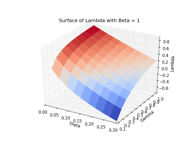
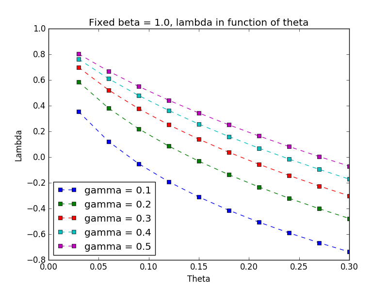
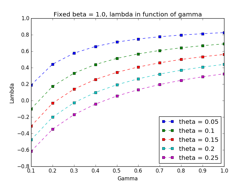
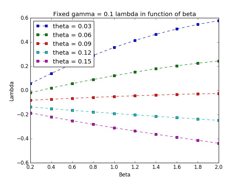
In this part, we give some examples about how our model and theorems can be applied to perform the numerical simulation of epidemics. The key quantity of our model is the Malthusian exponent . It dictates whether the infection will grow or vanish, and moreover serves as the growth or decay rate. We described how depends on in Proposition 6.1 and 6.3. However, the function is not explicit, so it is useful to investigate its values numerically. We use Finite Difference Method applied to (13) to approximate and then use (29) to approximate .
We simulated for different values of the three parameters in Figure 8. Figure 8(a) gives a surface of the function with , which confirms the monotonicity of on and (see also Figure 8(b) and Figure 8(c)). Thus to reduce infection, we should conduct more contact tracing (increase ) and avoid loss of contact information (decrease ). These two approaches are natural and intuitive.
Figure 8(d) confirms the monotonicity of on , see Proposition 6.3. When (thus ), is increasing on ; when (thus ), is a decreasing function of .
8 Complementary results and further discussions
In this part, we discuss some other properties and generalizations of our model.
8.1 Fragmentation by removing vertices
One can also consider a similar GFI process where the fragmentation is generated by removing vertices. We call the new process v-GFI process for short. More precisely, this process has the same dynamics of growth and isolation, but every vertex rings independently with an exponential clock of parameter , and once it rings, the associated vertex is removed from the cluster to generate several subclusters.
For the model of fragmentation by removing vertices on RRT (without isolation), some interesting properties about the size distribution have been discussed in [24]. Especially, a generalized splitting property should hold for our v-GFI process, so we can also follow the same strategy to study its size process . Moreover, by [24, eq.(7)] we deduce that the generator for the first moment semigroup of is
| (76) |
Compared to (14), we have , which implies that . Therefore we conclude that, quite surprisingly, and have exactly the same eigenelements given in Proposition 4.1, with a modification of Perron’s root . We can expect to recover other similar properties for the v-GFI process.
8.2 Role of the initial condition
Although the main results are proved with the initial condition (a patient zero), the proofs and results will not change much if the initial cluster is a RRT of any size. Indeed the reduction of the study to a growth fragmentation isolation process for sizes works similarly.
Besides, extension of the results to an initial condition given by a collection of RRTs can be achieved using that each initial cluster evolves independently by branching property.
Finally, one may wish to start from one (or a collection of) deterministic finite tree(s).We believe that our work can be adapted or used in that purpose. For instance using the stopping line when the clusters have size to exploit the results of this paper.
8.3 Model generalizations
We can use the same method to deal with generalizations such as allowing a cluster to lose several edges at the same time, or infect several individuals at the same time. More delicate generalizations could be interesting too:
- •
Adding recovering;
- •
Breaking the Markov property (adding an age would register the time for infection and would affect the individual rates in the epidemics: contamination, loss of contact information, and recovery);
- •
Improving and enriching the tracing procedure;
- •
Adding heterogeneity within the population (for tracing and infection).
The reduction we have exploited (from collections of trees to collection of sizes, due to the nice splitting property of RRT) should fail in general. We hope there is still some nice probabilistic constructions (even if more complex) to find but it is still speculative. We are confident on the extension of asymptotic results on the Malthusian growth and empirical measures. It could be achieved without going through a reduction of the state space and without describing the distribution of clusters at fixed times, but rather exploiting the general statement on semigroups that we have used here on a more complex state space (space of trees). In particular, the Lyapunov functions that we have exhibited here may still be relevant to deal with processes in more general state spaces.
8.4 Finite-distance contact tracing
In our model, the contact tracing is implemented for the whole cluster despite of its size, which is very rare in reality. It is natural to ask whether the properties observed in our model also hold for the finite-distance contact tracing. The answer is probably true, but the justification requires some new mathematical techniques.
A Conditional expectation and variance
We prove here Lemma 5.1 for the conditional expectation and variance estimates of
used in (50). Here , containing only growth and no fragmentation nor isolation, is a coupling of .
For the conditional expectation, we decompose it using the genealogy of clusters
| (77) |
We observe that for any ,
On the right hand side, the second term can be bounded by and the third term is zero, so we have
| (78) |
Since there is only growth in the process on , for any . So we can apply (78) with and to obtain that
| (79) |
For the first term on the right hand side in (79), we follow the proof of Lemma 4.1-(i) to get
For the second term in (79), we can control it by the total number of active clusters of size smaller than at that grow within :
For the conditional variance, we have
By branching property,
From the second line to the third line we use for any . The rest is the same as in the computation of conditional expectation and we obtain (52). ∎
B Coupling for modified GFI processes
We present here the details of the proof of Proposition 6.3. We will prove the monotone property Lemma 6.4 in Section B.1, which is divided into the part for size in Section B.1.1 and the part for waiting time in Section B.1.2. Then we apply this coupling along one cluster to the whole process in and prove Proposition 6.3 in Section B.2
Throughout this section, we fix , and two positive integers . Our object is a probability space as a coupling such that two modified GFI processes live in it: one is of parameters starting from an initial RRT of size , and the other is of parameters starting from an initial RRT of size . We denote by the size process of the former, and the size process of the latter. We will usually abuse these two notations to indicate the two modified GFI processes.
Recall the Ulam-Harris-Neveu notation defined in Section 3.1. For any cluster , its birth time is the moment when his parent makes the fragmentation, and its end of lifetime is the moment for its fragmentation or isolation event. During its lifetime, it has several growth events but the label is unchanged.
B.1 Coupling for one cluster
B.1.1 Coupling for the size distribution
As we said, the construction consists of the coupling of the event and the size distribution. We focus at first the later one, and study the passage of size domination between the generation.
Algorithm 1 (Coupling for the size distribution).
For the two modified processes and defined above and each cluster labeled appearing in , we use two independent random variables
to sample the fragmentation/isolation event when it comes to the end of lifetime. We denote by respectively for the size of in and at the end of its lifetime.
- 1.
If , the event is fragmentation in both processes. We then define
(80) and we set (resp. ) for the size of the first child cluster and the second child cluster in (resp. ).
- 2.
If , the event is isolation in both processes
We justify that this coupling of size gives us the desired passage of the size domination between the generation.
Proposition B.1.
Algorithm 1 is consistent with the fragmentation and isolation in the modified GFI process. Moreover, supposing , we also have the domination for the size of child clusters
| (81) |
As defined at the beginning of Section 6.3.1, the fragmentation and isolation are all attached to the edge in the modified GFI process. Then conditioned that an event is fragmentation or isolation, the probability to be fragmentation is , which is independent of its size. Moreover, following the splitting property 3.1, the event that a cluster of size has a second child of size can be sampled by
which is equivalent to (80). This proves the consistence of the coupling of size.
We then prove the size domination. Notice that the event type is same for the two processes, because it is determined by the common random variables . The domination thus (81) can be reduced to prove the following inequality: for every and two positive integers , we have
| (82) |
For the first inequality, we notice that
so it is increasing with respect to . For the second inequality, we have
From the second line to the third line, because , we have , , and “=” cannot be attained. Since the difference is an integer, this implies the second inequality in (82) and we finish the proof. ∎
B.1.2 Coupling for the waiting time
We now turn to the coupling of the waiting time, and aim to let larger cluster produce more growths within shorter lifetime. The main idea is a backward time-change sampling: we sample at first a pre-waiting time for the fragmentation/isolation event, which is generated by the current cluster size by supposing no growth events during its lifetime. Then we need to fill in the lifetime with the growth events, and make necessary time change with respect to the latest cluster size. After this time change, the pre-waiting time becomes the real waiting time of the fragmentation/isolation event.
Now, we give the detailed description of the backward time-change sampling in a modified GFI process of parameter .
Algorithm 2 (Backward time-change sampling).
For , we sample the events in its lifetime as following. Here all the random variables are independent. We denote by the cluster size of at birth.
- (i)
If , we apply the following steps:
- (i.1)
Set .
- (i.2)
Sample as the pre-waiting time from for the fragmentation/isolation event for . To unify the notation, we set as the pre-waiting time from .
- (i.3)
For any , suppose that we have already obtained for the -th growth event and as the pre-waiting time of the fragmentation/isolation from . We sample the -th growth event, whose waiting time from is sampled from a random variable . Then there are two cases.
- •
If , then the -th growth event happens before the fragmentation/isolation event. We set
(83) as the moment for the -th growth event. We also refresh the pre-waiting time for the fragmentation/isolation event from by
(84) - •
If , then there are only growth events before the fragmentation/isolation event. Therefore, we stop the recurrence of (i.3) and set
(85) as the length of lifetime of .
- •
- (i.1)
- (ii)
If at birth, we apply the following steps:
- (ii.1)
Sample for the waiting time of the first growth event of . Set .
- (ii.2)
Repeat step (i.2)-(i.3) for as a cluster of size .
- (ii.1)
This algorithm is also consistent with the modified GFI process thanks to the memory-less property of the exponential random variables. More precisely, we make use of Lemma B.1, which ensures that the time change in the step (i.3) gives us an new independent exponential random variable after the growth.
Lemma B.1.
For three independent random variables such that , with and , we have
It suffices to prove that, for any , we have
| (86) |
For the left-hand side, we have
By setting , we have
| (87) |
For the right-hand side of (86), we have
| (88) |
The advantage of Algorithm 2 is that the waiting time of fragmentation/isolation event largely depends on one random variable . This helps us construct a coupling to ensure the domination of lifetime length.
Algorithm 3 (Coupling of waiting time).
For any appearing in , let be respectively its size in and at birth. If , we have the following coupling for its evolution in two processes using Algorithm 2. Here for every quantity () in Algorithm 2, we keep its original notation for that in , and the notation with superscript () for that in .
- (i)
Sample two sets of random variables that
All the random variables are independent and they satisfy
The random variables in are used in both processes, while that in are only used in .
- (ii)
We use to generate the common randomness concerning the waiting time of fragmentation/isolation
(89) Here the indicator function comes from the fact that there is a supplementary growth event before sampling the fragmentation/isolation event in (ii) of Algorithm 2; we will also see them in the following paragraphs.
- (iii)
For the coupling of the growth events, we distinguish two cases.
- (iii.1)
If , then we use the random variable to generate the common randomness of growths for the two processes. That is, we set
(90) - (iii.2)
If , then our strategy is to let the growth in evolve independently until size , and then make coupling as (iii.1). That is, we let the first growth events in be sampled independently from that of using the random variables in
If all the growth events above are before the fragmentation/isolation event in , then the current cluster size of is also , and we let the rest of the the evolution of in be coupled with that in
(91) Otherwise, the number of growth is less than in and we only need the firth equation in (91) for the growth events in .
- (iii.1)
It is not hard to verify that Algorithm 3 gives a coupling of Algorithm 2. One only needs to check that all the random variables in Algorithm 3 have the proper parameters as in Algorithm 2. Meanwhile, some common random variables create correlations between the processes and this is the object of the coupling. As we said, thanks to the backward time-change sampling, we only need to sample one exponential random variable for the waiting time of fragmentation/isolation, and it is quite natural to use a common random variable to create monotonicity. It is also the idea for the growth events, but the case is a little more delicate.
Proposition B.2.
Let appearing in , and suppose two positive integers be respectively its size in and at birth. Then in Algorithm 3, the length of lifetime is shorter in than that in , and its size at the end of lifetime is also larger in the former process.
Before proving Proposition B.2, one intermediate step is to define a predicted length of lifetime after -th growth, as a generalization of (85) in Algorithm 2
| (92) |
The interpretation is that we have explored the information of events until the moment , and suppose no more growth event after it. Thus we make a sum of and . Heuristically, the more growth events we explore, the closer to this quantity is. We justify this observation.
Lemma B.2.
Let be the cluster size of at birth and be the number of growth events after in Algorithm 2, then we have an expression that for every
| (93) |
Moreover, the sequence is decreasing.
The indicator here is used to distinguish the special case in Algorithm 2. We prove (93) for the case at first by recurrence. The case is trivial by the expression that
Suppose that we have proved the case for , then for the case we apply the formula (83) and (84)
| (94) |
We then apply the recurrence of (93) at and obtain
This is the desired result of (93). For the monotonicity, we apply the recurrence (94).
By (i.3) of Algorithm 2, the existence of -th growth implies . Therefore, the difference above is negative and we finish the proof.
Then for the case , it suffice to add the first growth event at , and treat the rest term as the evolution of a cluster of size . ∎
We treat the two cases in the step (ii) of Algorithm 3.
- 1.
For the case , the coupling in (89) and (90) gives us that
(95) thanks to the fact and they use the same random variables in . This implies in Algorithm 2 that the waiting time for each growth event is always shorter in , while the pre-waiting time for the fragmentation/isolation event are same. By an induction in (84), we also establish , which ensures that we can explore more growth events in . This finishes the statement about the size in Proposition B.2 for the case .
Concerning the length of lifetime, we use the formula (93) of the -th predicted length of lifetime that
Compare it with its version in , we have
because of (95). This implies that . As we know, there exists a such that , so we have
Here the last inequality comes from the decreasing property in Lemma B.2 and the fact there are more growth events in . This finishes the statement about the length of lifetime in Proposition B.2 for the case .
- 2.
For the case , there are also two cases.
- a)
There are less than growth events for in . For this case, the statement about the size is obvious as the cluster size is less than in of at the end of lifetime. We consider the length of lifetime in that
In the last line, we make use of (89). Notice that is the cluster size of after several growth events in its lifetime, and it should be less than by assumption. Thus, we obtain
where the last inequality comes from the decreasing property in Lemma B.2. We choose as the index of the last growth event of in , and this concludes the statement about the length of lifetime.
- b)
There are at least growth events for in . From (ii).b of Algorithm 3, after growth events, has the same cluster size in two processes and the growth events are totally coupled. Equation (91) gives us
(96) thus the domination of waiting time for the growth events is also established. For the pre-waiting time of the fragmentation/isolation event, (84) gives us
So a telescope formula entails
(97) Here we use the the fact that are sampled by the same random variable in (89). Therefore, (97) also gives us a domination of the pre-waiting time that . Combining this with (96), we can make use of a similar argument like the case for the part of in after growth events, together with in from its birth. This concludes our proof.
- a)
∎
B.2 Complete proof of Proposition 6.3
We can now apply the coupling in previous sections to the whole process and , which gives us desired property in the previous discussion in Section 6.3.
Algorithm 4 (Coupling for modified GFI processes).
Recall the Ulam-Harris-Neveu notation defined in Section 3.1, where we use for the labels of the alive clusters at moment , for the one issued from and for the cluster size of label . We keep the original version for the process and for its version in . The following proposition captures the intuition that “ evolves quicker than , and for every cluster the processes are no longer coupled from a certain random time”.
Proposition B.3.
The probability space defined in Algorithm 4 satisfies the following properties.
- •
and live in it as a modified GFI process with respect to their natural filtration.
- •
Under the filtration defined as
(99) for every , there exists a stopping time with respect to such that and is Markov process with respect to the filtration .
The first statement is the result of the recurrence of Algorithm 1 and 3. In this recurrence, Proposition B.2 ensures the monotonicity of the length of lifetime and cluster size when fragmentation, while Proposition B.1 pass this monotonicity to the child clusters. Therefore, evolves quicker than .
Concerning the second statement, when a cluster of label stops its evolution at in , its trajectory translates to the information about , which then translates to its coupled one in : it is still alive at a moment . This dependence implies that is a stopping time with respect to . Naturally, for the rest of process after , because does not provide more information and then we obtain the Markov property. Thus we finish the proof of the second statement. ∎
We use respectively for the expectation on the probability space of and . Our main object is to compare and , which will illustrate Malthusian behavior for large .
We use the common probability space constructed in Algorithm 4, and we write for the associated expectation. By Proposition B.3, under , every cluster in has its coupled one in , which is still alive at the moment and produces the clusters in . Then we have
Since the modified GFI process is càdlàg, we apply the strong Markov property that
and the quantity can be seen as the mean of offspring for a modified GFI process issued from a RRT of size .
Lemma 6.3 gives us some indication about the phases of the modified GFI process, but here we need a more precise result. In fact, the mapping is increasing (resp. decreasing) when (resp. ). The idea is to use the first moment generator (73) and a constant test function that
Therefore, the sign depends on . For the case , we obtain
and from this we deduce
| (100) |
Because of the Malthusian behavior (29), for a large we have
where are the associated eigenvectors. The monotonicity (100) thus implies for the case :
- •
when , we have ;
- •
when , we have .
The case is similar. Finally, recall as discussed in Section 6.3.1, we thus obtain the desired result. ∎
References
- [1] [author] Akian, MarianneM., Ganassali, LucaL., Gaubert, StéphaneS. and Massoulié, LaurentL. (2020). Probabilistic and mean-field model of COVID-19 epidemics with user mobility and contact tracing. arXiv preprint arXiv:2009.05304.
- [2] [author] Asmussen, SorenS. and Hering, HeinrichH. (1976). Strong limit theorems for general supercritical branching processes with applications to branching diffusions. Z. Wahrscheinlichkeitstheorie und Verw. Gebiete 36 195–212. 10.1007/BF00532545 420889
- [3] [author] Athreya, K. B.K. B. (2012). Coalescence in the recent past in rapidly growing populations. Stoch. Proc. Appl. 122 3757–3766.
- [4] [author] Athreya, Krishna BalasundaramK. B. (1968). Some results on multitype continuous time Markov branching processes. Ann. Math. Statist. 39 347–357. 10.1214/aoms/1177698395 221600
- [5] [author] Ball, FrankF. and Donnelly, PeterP. (1995). Strong approximations for epidemic models. Stochastic Process. Appl. 55 1–21. 10.1016/0304-4149(94)00034-Q 1312145
- [6] [author] Bansaye, VincentV., Cloez, BertrandB. and Gabriel, PierreP. (2020). Ergodic behavior of non-conservative semigroups via generalized Doeblin’s conditions. Acta Appl. Math. 166 29–72. 10.1007/s10440-019-00253-5 4077228
- [7] [author] Bansaye, VincentV., Cloez, BertrandB., Gabriel, PierreP. and Marguet, AlineA. (2022). A non-conservative Harris’ ergodic theorem. J. London Math. Soc. 2 1–52.
- [8] [author] Bansaye, VincentV., Delmas, Jean-FrançoisJ.-F., Marsalle, LaurenceL. and Tran, Viet ChiV. C. (2011). Limit theorems for Markov processes indexed by continuous time Galton-Watson trees. Ann. Appl. Probab. 21 2263–2314. 10.1214/10-AAP757 2895416
- [9] [author] Barlow, Martin TM. T. A branching process with contact tracing. Preprint 2020 available via https://www.math.ubc.ca/ barlow/preprints/112-bpct5.pdf.
- [10] [author] Baur, ErichE. and Bertoin, JeanJ. (2014). Cutting edges at random in large recursive trees. In Stochastic analysis and applications 2014. Springer Proc. Math. Stat. 100 51–76. Springer, Cham. 10.1007/978-3-319-11292-3_3 3332709
- [11] [author] Bertoin, JeanJ. (2012). Fires on trees. Ann. Inst. Henri Poincaré Probab. Stat. 48 909–921. 10.1214/11-AIHP435 3052398
- [12] [author] Bertoin, JeanJ. (2017). Markovian growth-fragmentation processes. Bernoulli 23 1082–1101. 10.3150/15-BEJ770 3606760
- [13] [author] Bertoin, JeanJ. (2022). A model for an epidemic with contact tracing and cluster isolation, and a detection paradox. arXiv preprint arXiv:2201.01924.
- [14] [author] Bertoin, JeanJ. and Watson, Alexander RA. R. (2018). A probabilistic approach to spectral analysis of growth-fragmentation equations. J. Funct. Anal. 274 2163–2204. 10.1016/j.jfa.2018.01.014 3767431
- [15] [author] Bertoin, JeanJ. and Watson, Alexander R.A. R. (2020). The strong Malthusian behavior of growth fragmentation processes. Ann. H. Lebesgue 3 795-823.
- [16] [author] Cormen, Thomas H.T. H., Leiserson, Charles E.C. E., Rivest, Ronald L.R. L. and Stein, CliffordC. (2009). Introduction to algorithms, Third ed. MIT Press, Cambridge, MA. 2572804
- [17] [author] Du, MarvinM. (2022). Contact tracing as a measure to combat COVID-19 and other infectious diseases. American Journal of Infection Control 50 638–644.
- [18] [author] Engländer, JánosJ., Harris, Simon C.S. C. and Kyprianou, Andreas E.A. E. (2010). Strong law of large numbers for branching diffusions. Ann. Inst. Henri Poincaré Probab. Stat. 46 279–298. 10.1214/09-AIHP203 2641779
- [19] [author] Fetzer, ThiemoT. and Graeber, ThomasT. (2021). Measuring the scientific effectiveness of contact tracing: Evidence from a natural experiment. Proceedings of the National Academy of Sciences 118 e2100814118.
- [20] [author] Gu, ChenlinC., Jiang, WeiW., Zhao, TianyuanT. and Zheng, BanB. (2020). Mathematical recommendations to fight against COVID-19. Available at SSRN 3551006.
- [21] [author] Harris, SimonS., Horton, EmmaE. and Kyprianou, AndreasA. (2020). Stochastic Methods for the Neutron Transport Equation II: Almost Sure Growth. Ann. Appl. Probab. 30 2815-2845.
- [22] [author] Harris, Simon CS. C., Johnston, Samuel GGS. G. and Roberts, Matthew IM. I. (2020). The coalescent structure of continuous-time Galton–Watson trees. Ann. Appl. Probab. 30 1368–1414.
- [23] [author] Horton, EmmaE. and Watson, Alexander RA. R. (2020). Strong laws of large numbers for a growth-fragmentation process with bounded cell sizes. arXiv preprint arXiv:2012.03273.
- [24] [author] Kalay, Z.Z. and Ben-Naim, E.E. (2015). Fragmentation of random trees. J. Phys. A 48 0405001, 15. 10.1088/1751-8113/48/4/045001 3300251
- [25] [author] Keeling, Matt JM. J., Hollingsworth, T DeirdreT. D. and Read, Jonathan MJ. M. (2020). Efficacy of contact tracing for the containment of the 2019 novel coronavirus (COVID-19). J Epidemiol Community Health 74 861–866.
- [26] [author] Kesten, H.H. and Stigum, B. P.B. P. (1966). A limit theorem for multidimensional Galton-Watson processes. Ann. Math. Statist. 37 1211–1223. 10.1214/aoms/1177699266 198552
- [27] [author] Kurtz, ThomasT., Lyons, RussellR., Pemantle, RobinR. and Peres, YuvalY. (1997). A conceptual proof of the Kesten-Stigum theorem for multi-type branching processes. In Classical and modern branching processes (Minneapolis, MN, 1994). IMA Vol. Math. Appl. 84 181–185. Springer, New York. 10.1007/978-1-4612-1862-3_14 1601737
- [28] [author] Lambert, AmauryA. (2021). A mathematical assessment of the efficiency of quarantining and contact tracing in curbing the COVID-19 epidemic. Math. Mod. Nat. Phen. 16.
- [29] [author] Marguet, AlineA. (2019). A law of large numbers for branching Markov processes by the ergodicity of ancestral lineages. ESAIM Probab. Stat. 23 638–661. 10.1051/ps/2018029 4011569
- [30] [author] Marzouk, CyrilC. (2016). Fires on large recursive trees. Stochastic Process. Appl. 126 265–289. 10.1016/j.spa.2015.08.006 3426519
- [31] [author] Meir, A.A. and Moon, J.J. (1974). Cutting down recursive trees. Bellman Prize in Mathematical Biosciences 21 173-181.
- [32] [author] Meyn, Sean P.S. P. and Tweedie, R. L.R. L. (1993). Stability of Markovian processes. III. Foster-Lyapunov criteria for continuous-time processes. Adv. in Appl. Probab. 25 518–548. 10.2307/1427522 1234295
- [33] [author] Mischler, S.S. and Scher, J.J. (2016). Spectral analysis of semigroups and growth-fragmentation equations. Ann. Inst. H. Poincaré Anal. Non Linéaire 33 849–898. 10.1016/j.anihpc.2015.01.007 3489637
- [34] [author] Tomasevic, MilicaM., Véber, AmandineA. and Bansaye, VincentV. (2020). Ergodic behaviour of a multi-type growth-fragmentation process modelling the mycelial network of a filamentous fungus. Available via https://hal.inria.fr/hal-03087196.