Anomalous Magnetic Moment and Higgs Coupling of the Muon in a Sequential U(1) Gauge Model with Dark Matter
Abstract
We study an Abelian gauge extension of the standard model with fermion families having non-universal gauge charges. The gauge charges and scalar content are chosen in such an anomaly-free way that only the third generation fermions receive Dirac masses via renormalisable couplings with the Higgs boson. Incorporating additional vector like fermions and scalars with appropriate charges can lead to radiative Dirac masses of first two generations with neutral fermions going in the loop being dark matter candidates. Focusing on radiative muon mass, we constrain the model from the requirement of satisfying muon mass, recently measured muon anomalous magnetic moment by the E989 experiment at Fermilab along with other experimental bounds including the large hadron collider (LHC) limits. The anomalous Higgs coupling to muon is constrained from the LHC measurements of Higgs to dimuon decay. The singlet fermion dark matter phenomenology is discussed showing the importance of both annihilation and coannihilation effects. Incorporating all bounds lead to a constrained parameter space which can be probed at different experiments.
I Introduction
Recently, the E989 experiment at Fermilab has measured the anomalous magnetic moment (AMM) of muon, = , showing a discrepancy with respect to the theoretical prediction of the Standard Model (SM) Abi:2021gix
| (1) | |||
| (2) |
When combined with the previous Brookhaven determination
| (3) |
it leads to a 4.2 observed excess of 11 1 It should however, be noted that the latest lattice results Borsanyi:2020mff predict a larger value of muon bringing it closer to experimental value. Tension of measured muon with global electroweak fits from to hadron data was also reported in Crivellin:2020zul; Colangelo:2020lcg; Keshavarzi:2020bfy.. The theoretical status of SM calculation of muon AMM can be found in Aoyama:2020ynm. While this anomaly is known for a long time since the Brookhaven measurements Muong-2:2001kxu, the recent Fermilab measurements have also led to several recent works on updating possible theoretical models with new data, a comprehensive review of which may be found in Athron:2021iuf. Earlier reviews on this topic can be found in Jegerlehner:2009ry; Lindner:2016bgg.
In this work, we consider an anomaly free gauge extension of the SM where first two generations of charged fermions acquire masses only at radiative level. While triangle anomalies cancel due to addition of chiral fermion triplets, giving rise to type III seesaw origin of light neutrino masses, the new fields introduced for radiative charged fermion masses can also serve as a stable dark matter (DM) candidate, if it is stable and neutral. Focusing primarily on radiative muon mass and muon AMM, we constrain the model from the requirement of satisfying muon mass, latest muon data along with other relevant bounds like the Higgs coupling to muons as measured by the large hadron collider (LHC), Higgs to diphoton bound as well as direct search bounds on beyond standard model (BSM) particles. We also constrain the model from the requirement of generating the desired DM phenomenology. Radiative charged lepton mass in the context of AMM have been a topic of interest for many years and several interesting works have already appeared in the literature within supersymmetric Borzumati:1999sp; Czarnecki:2001pv; Crivellin:2010ty; Thalapillil:2014kya as well as non-supersymmetric frameworks Fraser:2014ija; Fraser:2015zed; Calibbi:2020emz; Yin:2021yqy; Chiang:2021pma; Baker:2021yli. On the other hand, connection between dark matter and muon have also been studied in several earlier works, but with tree level muon mass Calibbi:2018rzv; Kawamura:2020qxo; Chen:2020tfr; Jana:2020joi; Kowalska:2017iqv; Kowalska:2020zve; Arcadi:2021cwg; Chowdhury:2021tnm.
We provide a natural origin of muon AMM together with radiative muon mass and dark matter in a sequential gauged model that can also explain light neutrino mass from type III seesaw. The particle content and the corresponding charge assignments are chosen in such an anomaly free way that additional global symmetries are not required. The radiative muon mass leads to anomalous Higgs coupling to muon which can be probed at the LHC. In spite of having several BSM particles and free parameters, we find the model to be highly constrained from the requirements of satisfying relevant constraints.
This paper is organised as follows. In section II, we briefly discuss the model. In section III, we discuss the possible origin of muon in this model followed by discussion of electroweak precision constraints in section IV. We briefly comment upon electric dipole moment and lepton flavour violation constraints in section V followed by discussion of collider constraints in section VI. In section VII we discuss DM details and summarise our results in section VIII.
II The Model
| Particle | ||
|---|---|---|
The fermion content of the minimal model is shown in table 1. The charges correspond to anomaly-free combination with being arbitrary with . While such Abelian extension of the standard model was studied before Ma:2002pf; Barr:2005je; Adhikari:2008uc; Adhikari:2015woo; Bhat:2019yqo in different contexts, recently the possibility of having a sequential with different quantum numbers for each family was proposed Ma:2021aag. As an working example, for all three families while for first, second and third families respectively were chosen. Now, if just one scalar doublet is chosen having zero charge and responsible for electroweak symmetry breaking, only the third generation quarks and charged leptons can acquire masses at renormalisable level22 2 See Balakrishna:1987qd; Balakrishna:1988ks; Ma:1990ce; Barr:1989ta; Babu:1988fn; Weinberg:2020zba for earlier discussions on fermion mass hierarchy through sequential loop suppression.. The field content of the minimal model with such choices of is shown in table 2. As discussed in Ma:2021aag, such a minimal setup leads to tree level third generation charged fermion masses while the first and second generation masses arise only at dimension six and dimension five levels, leading to natural suppression.
| Particle | ||
|---|---|---|
Clearly, one can consider additional field content in order to provide a UV complete realisation for such higher dimensional operators for first and second generation masses. For example, muon mass can arise at one-loop level, in scotogenic fashion Ma:2006km, after introducing the particles shown in table 3. The corresponding one-loop diagram is shown in figure 1.
| Particle | ||
|---|---|---|
Similarly, additional fields can be introduced to generate other charged fermion as well as Dirac neutrino masses of first and second generations at radiative level. Here we focus only the new physics responsible for muon mass origin at one-loop in the context of dark matter, muon and LHC constraints. The relevant part of the Lagrangian for muon mass is given by
| (4) |
As noticed from the above Lagrangian, the newly introduced fields for scotogenic muon mass, always appear in pairs of the form . This is due to the chosen charge assignments of these fields. Therefore, the Lagrangian possesses a global symmetry under which the fields shown in table 3 can have non-trivial transformations while the SM fields transform trivially Ma:2021aag. As none of the scalar fields in table 3 acquire any vacuum expectation value (VEV), this symmetry remains unbroken, keeping the lightest particle with non-trivial charge stable and hence the DM candidate.
The one-loop muon mass can be estimated as
| (5) |
where are physical masses of scalars in loop, which can be derived by diagonalising the charged scalar mass matrix given in Appendix A. Here denote the VEV of the neutral component of the SM Higgs doublet and singlet scalar respectively. The physical mass eigenstates arise due to mixing of by angle given by
| (6) |
The loop function is given by
| (7) |
where , . The effective coupling of the SM Higgs to muon can be calculated from the same muon mass diagram as
| (8) |
where
For details of other fermion masses including neutrinos, one may refer to Ma:2021aag. The physical scalar spectrum and the couplings are given in Appendix A. Clearly, the muon coupling to the SM Higgs gets changed from the usual SM value to the one shown in equation (8) above. As can be seen from the full scalar potential of the model given in Appendix A, in addition to term discussed above, there exist other quartic couplings of SM Higgs with scalars like . Since also couple to muons, such additional quartic couplings can also lead to anomalous Higgs coupling to muons without contributing to muon mass at one-loop. However, we have considered such additional quartic couplings to be small so that dominant contribution to muon anomalous coupling to Higgs arises from the same quartic coupling which also gives rise to radiative muon mass as discussed above. This anomalous muon coupling to the SM Higgs can be constrained from the LHC observations as we discuss in one of the upcoming sections. While there is no role of singlet scalar in muon mass generation at one-loop, it is required to generate other fermion masses within a minimal setup as discussed in Ma:2021aag. Considering the VEV of to be , the mass of gauge boson after symmetry breaking is .
III Muon Anomalous Magnetic Moment
As mentioned before, there is a discrepancy between muon AMM predictions of theory and experimental measurements and can potentially be explained with BSM physics. In the gauge model we discuss here, there are two different contributions to muon : one from charged scalars in the loop and another where gauge boson goes in the loop. While the contribution from gauge boson loop is sub-dominant for typical TeV scale masses, the contribution from charged scalar loop can be enhanced. This is because, the same loop particles also give rise to muon mass thereby removing the additional loop factor from muon contributions Fraser:2015zed. Similar discussions on muon in radiative muon mass models have also appeared recently in Baker:2021yli. The charged scalar loop contribution to muon in our model is shown in figure 2 where are the mass eigenstates of after symmetry breaking. The corresponding contribution to muon is given by Baker:2021yli
| (9) |
The neutral gauge boson contribution to muon AMM (shown in figure 3) can be written as Brodsky:1967sr; Baek:2008nz; Queiroz:2014zfa
| (10) |
where . As shown in earlier works Bauer:2018onh; Borah:2020jzi; Borah:2021jzu; Borah:2021mri; Borah:2021khc, the only allowed region where such neutral gauge boson contribution can explain muon AMM is in the sub-GeV regime with corresponding gauge coupling smaller than . Since we consider heavy gauge boson limit, the contribution from such neutral gauge bosons remain suppressed. In fact, since gauge boson couples to electrons as well, the bounds from low energy experiments related to dark photon searches are likely to rule out the low mass regime completely Bauer:2018onh leaving us with the explanation of muon AMM from charged scalar loop only.
An important observation about muon g-2 is that if the muon mass originates at tree level, as in the SM, then a loop contribution from a scalar and a fermion is positive if the scalar (fermion) is neutral (charged), but negative if the scalar (fermion) is charged (neutral). However, if the muon mass is radiative in one-loop coming from a scalar and a fermion as in our model, then the sign reverses. Therefore, even with charged scalar loop shown in figure 2, we can still explain positive .
IV Electroweak Precision Constraints
Another constraint on the model parameters can arise due to the electroweak precision data (EWPD) encoded in Peskin-Takeuchi oblique parameters S and T. Due to the presence of new scalar doublet () and charge singlet scalar (), these oblique parameters can receive additional contributions. As shown in Grimus:2008nb; Cao:2017ffm, the charged singlet scalar () contributes to the S parameter only and does not affect the T parameter at one loop level. Also, the corresponding contribution of singlet scalar remains small, well within error bars. The contributions due to the scalar doublet () can be written asJueid:2020rek
| (11) | ||||
where is the loop function and can be expressed as
The present best fit values of and ParticleDataGroup:2018ovx can be used for deriving the constraint on the model parameters as we discuss in upcoming sections.
V Electric dipole moment and lepton flavour violation
Similar to the anomalous magnetic moment discussed above, electric dipole moment (EDM) of leptons is a flavour conserving observable which is a measure of the coupling of the lepton’s spin to an external electric field. In the SM, lepton EDMs are vanishingly small and hence any experimental observation can be a clear sign of BSM physics. While in the SM, EDM of lepton like muon arises only at four loop level, in the present model, we can have muon EDM at one-loop level itself via a diagram similar to the one-loop diagrams for muon . Since one-loop contribution to muon EDM can be sizeable, one can constrain the model parameters from experimental bound Muong-2:2008ebm
| (14) |
However, EDM is a CP violating observable and hence depends upon CP violating couplings involved in the one-loop process Borah:2017leo. Since rest of our analysis does not rely upon new sources of CP violation, we can tune them appropriately to keep the resulting EDM within experimental limit.
Another flavour observable is related to charged lepton flavour violation (CLFV) like which can naturally arise in BSM scenarios like radiative mass models. Experimental constraints on this rare decay process at confidence level MEG:2016leq can be used to constrain the parameter space of such models. In order to realise such flavour violating decays, the particles in the loop need to couple to different generations of fermions. However, due to non-universal charges in our model, the fields responsible for radiative muon mass as well as muon , do not couple to other lepton generations. Therefore, we do not have such one-loop CLFV processes and hence they do not impose any additional constraints on the parameter space.
VI Collider Constraints
Collider constraints can primarily apply on SM Higgs decay into muons as the effective coupling is changed in such radiative muon mass models. Additional constraints can apply to physical masses of charged scalars as well as other particles having electroweak interactions from direct search bounds. The modifications in Higgs decay into muons, relative to the SM can be written the corresponding ratio of branching fractions as
| (15) |
as given by the CMS collaboration Sirunyan:2020two. Similar bound has been reported by the ATLAS collaboration Aad:2020xfq as well.
Higgs to diphoton rate in the model including SM contribution and new charged scalars is given byDjouadi:2005gi
| (16) |
where is Fermi coupling constant, is fine structure constant, is the color factor of charged fermion in loop, are electromagnetic charges of fermions and scalars in loop and with running over all charged particles in loop. The form factors for fermion, vector boson and scalars are given by
The function is given by
The parameter denotes SM Higgs coupling with the charged scalar . They are given by :
where is the mixing angle for and as given by Eq. (6). The first two couplings are relevant for . The first two terms in Eq. (16) are due to SM contributions and the last term is due to charged scalars in extra gauge model. So new contributions to come from the last term and its interference with SM terms.
According to the the latest CMS results Sirunyan:2021ybb, the constraints on Higgs to diphoton ratio is which implies the new contribution should satisfy the constraint
| (17) |
Similarly, collider bounds exist on neutral gauge boson mass and corresponding gauge couplings. The limits from LEP II data constrains such additional gauge sector by imposing a lower bound on the ratio of new gauge boson mass to the new gauge coupling TeV Carena:2004xs; Cacciapaglia:2006pk. The bounds from ongoing LHC experiment have already surpassed the LEP II bounds. In particular, search for high mass dilepton resonances have put strict bounds on such additional gauge sector coupling to all generations of leptons and quarks with coupling similar to electroweak ones. The latest bounds from the ATLAS experiment Aaboud:2017buh; Aad:2019fac and the CMS experiment Sirunyan:2018exx at the LHC rule out such gauge boson masses below 4-5 TeV from analysis of 13 TeV data. Such bounds get weaker, if the corresponding gauge couplings are weaker Aaboud:2017buh than the electroweak gauge couplings. Also, if the gauge boson couples only to the third generation of leptons, all such collider bounds become much weaker, as explored in the context of DM and collider searches in a recent work Barman:2019aku. Similarly, additional scalar sector can also be constrained from collider data. While there are no dedicated LHC searches for singlet charged scalar (like in our model) yet, theoretical studies like Alcaide:2019kdr show high luminosity LHC sensitivity upto 500 GeV. For electroweak doublet like , LEP II bounds rule out some part of the parameter space below 100 GeV Lundstrom:2008ai. At colliders, if they are produced, they can decay into DM (missing energy) as well as charged leptons (say, muon). Such leptonic final states with missing energy have been studied in several earlier works Miao:2010rg; Gustafsson:2012aj; Datta:2016nfz. As a conservative lower limit, we consider all such BSM scalars to be heavier than 100 GeV in our numerical analysis.
VII Dark Matter
The neutral singlet vector like fermion is the dark matter candidate in this model. Although neutral component of the scalar doublet could also be a DM candidate, it turns out that the neutral components of are degenerate leading to a large boson mediated DM-nucleon scattering, ruled out by experiments like XENON1T Aprile:2018dbl. The situation is similar to sneutrino DM in minimal supersymmetric standard model (MSSM) Arina:2007tm. This leaves us with the only choice of fermion singlet being the DM candidate. Since it does not interact with any singlet scalar, so DM phenomenology is dictated by its annihilation via gauge boson only. While for such pure gauge mediated annihilations, the relic is likely to be satisfied near the resonance region , for small mass splitting between DM and charged scalars one can have interesting coannihilation effects which depends upon Yukawa couplings dictating both muon mass and .
The relic abundance of a dark matter particle , which was in thermal equilibrium at some earlier epoch can be calculated by solving the Boltzmann equation
| (18) |
where is the number density of the dark matter particle and is the number density when was in thermal equilibrium. is the Hubble expansion rate of the Universe and is the thermally averaged annihilation cross section of the dark matter particle . In terms of partial wave expansion . Numerical solution of the Boltzmann equation above gives Kolb:1990vq; Scherrer:1985zt
| (19) |
where , is the freeze-out temperature, is the mass of dark matter, is the number of relativistic degrees of freedom at the time of freeze-out and and GeV is the Planck mass. Dark matter particles with electroweak scale mass and couplings freeze out at temperatures approximately in the range . More generally, can be calculated from the relation
| (20) |
which can be derived from the equality condition of DM interaction rate with the rate of expansion of the Universe . The thermal averaged annihilation cross section used in Boltzmann equation of (18) is given by Gondolo:1990dk
| (21) |
where ’s are modified Bessel functions of order , is the mass of Dark Matter particle and is the temperature.
If there exists some additional particles having mass difference close to that of DM, then they can be thermally accessible during the epoch of DM freeze out. This can give rise to additional channels through which DM can coannihilate with such additional particles and produce SM particles in the final states. This type of coannihilation effects on dark matter relic abundance were studied by several authors in Griest:1990kh; Edsjo:1997bg; Bell:2013wua. As we will see while incorporating all relevant constraints, there exist regions of parameter space where DM fermion can have small mass splitting with charged scalars leading to a region of strong coannihilations. Since the corresponding Yukawa couplings are also required to be large to satisfy other bounds, such coannihilations can in fact lead to suppressed relic abundance. We use the package micrOMEGAs Belanger:2013oya to calculate DM relic abundance in the most general way and use FeynRules Alloul:2013bka package to prepare the required model files.
VIII Results and Conclusion
Let us now discuss all possible phenomenological consequences of our model. We will consider the constraints coming form the AMM of muon, muon mass, the decay of SM Higgs to and , and finally the relic abundance of DM respectively. The important parameters for these different observable are the following:
However, all the other observable are independent of and except the relic density of DM and we will discuss the role of these parameters first. In figure 4, we have shown the allowed parameter space in vs plane, from muon mass (blue line), muon (the brown band), (vertical green band) and (the grey mesh). We have fixed all the other parameters according to the BP-1 shown is table 4 and one can clearly see that all these different regions coincide with each other in a very tiny region in vs plane.
In figure 5, we have shown the allowed parameter space in the same vs plane by varying all the other parameters as mentioned in table 5. In the left panel, the color code represents the mass splitting between the and where as in the right panel, the color code shows the variation of the Yukawa coupling . For simplicity, we have assumed equality of Yukawa couplings . Any deviation from this equality is unlikely to bring substantial change in our results. In spite of the presence of many different parameters, a very small region of parameter space is allowed from all the above-mentioned constraints. One can also note that we require quite large () to satisfy all possible constraints. Finally, we have shown the constraints coming from the electroweak precision observable as discussed in section IV. A very small region of the parameter space is excluded from the EWPD constraints33 3 Note that we have made a conservative estimate by considering a pure scalar doublet contribution. The actual estimate will involve both doublet and singlet scalar contributions with possible interference, a full calculation of which is beyond the scope of present work. as shown in the black and red coloured points in the high mass regime of charged scalar in figure 5. While the band consisting of coloured points satisfy all relevant bounds, the upper half of the plane (shaded) is disfavoured as it corresponds to unstable DM candidate.


| Benchmark points | ||||||||
|---|---|---|---|---|---|---|---|---|
| (GeV) | (GeV) | (GeV) | (GeV) | |||||
| BP-1 | 200-3000 | 71.43 | 200-5000 | 0.8741 | 0.6756 | -0.8327 | ||
| BP-1/2 | + 15 | + 10 | 500-3000 | 0.887 | 0.792 | -0.862 | 0.009 | 2813 |
| BP-2/2 | + 105 | + 100 | 500-3000 | 0.887 | 0.792 | -0.862 | 0.009 | 2813 |
| BP-3/2 | + 255 | + 250 | 500-3000 | 0.887 | 0.792 | -0.862 | 0.009 | 2813 |
| BP-1/3 | + 15 | + 10 | 500-3000 | 0.9156 | 0.644 | -0.282 | 0.038 | 2447 |
| BP-2/3 | + 105 | + 100 | 500-3000 | 0.9156 | 0.644 | -0.282 | 0.038 | 2447 |
| BP-3/3 | + 605 | + 600 | 500-3000 | 0.9156 | 0.644 | -0.282 | 0.038 | 2447 |
| Parameters | Range |
|---|---|
| (100 GeV, 5 TeV) | |
| (1 GeV, 500 GeV) | |
| (1 GeV, 10 TeV) | |
| (0.01, 1) | |
| (0.01, ) | |
| (-0.001, -1) |
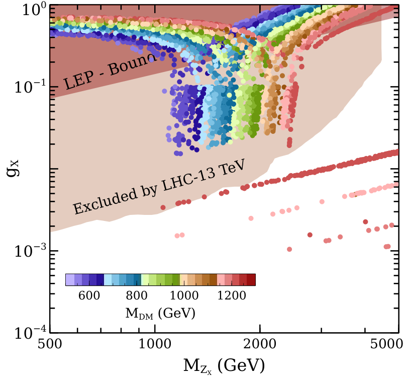
So far, we have not taken into account the constraints coming from the observed relic density of DM. As discussed earlier, the DM particles freeze-out from the thermal bath due to the annihilation and co-annihilation processes through the new Yukawa as well as gauge interactions. Figure 6 represents the relic abundance of DM as a function of its mass () and all the other parameters have been kept fixed according to the benchmark points shown is table 4. We have chosen these benchmark points from allowed region shown in figure 5 so that all other constraints are satisfied. The left panel is for very small whereas the right panel is for slightly larger . One can clearly notice the absence (presence) of resonance in the left (right) panel due to the smallness (largeness) of the gauge coupling . Finally, we have shown the role of both and in figure 7. Here, we have shown the allowed parameter space in versus plane, while other parameters are kept fixed at benchmark points allowed from all possible experimental constraints. We consider the allowed points for DM masses as shown in figure 5 and then vary randomly in the range shown in figure 7. The scattered points in figure 7 correspond to DM masses (shown in colour bar) which satisfy correct relic abundance. The effect of DM annihilation mediated by is clearly visible for masses close to resonance regime while the points away from resonance will satisfy relic due either due to large gauge coupling or coannihilation with scalars. The grey shaded region in figure 7 corresponds to the exclusion limits from the LHC searches for heavy resonances decaying into lepton pairs Aaboud:2017buh; Aad:2019fac; Sirunyan:2018exx. The brown shaded region corresponds to the LEP bound TeV. The most important point to note here is that the LHC-13 TeV data excludes a broad region of parameter space of our model. In order to implement the LHC bound we compute the dilepton production cross section at 13 TeV center of mass energy at the LHC using the package MADGRAPH Alwall:2014hca. As the first generation quarks have charges more than unity, we get a stricter bound on parameter space compared to other universal Abelian extensions like gauged . Clearly, the benchmark points shown in the last three rows of table 4 are already disallowed by the LHC bounds. In fact, only a handful of DM masses from Fig. 5 survive LHC bounds, as shown in Fig. 7. Due to constant DM mass but varying , many of these points seem to fall on a line in the allowed region of Fig. 7. With a much bigger scan size, the allowed region can be filled with more points allowed from all relevant constraints. Clearly, all these allowed points correspond to small values of gauge coupling and hence coannihilation effects play dominant role in generating correct DM relic. The mass splitting of DM and scalars are in the range of 150-500 GeV while the corresponding Yukawa couplings are of order unity leading to efficient coannihilations for DM masses in 1200-1500 GeV range falling in the allowed region. We also check that the points allowed by LHC bounds are also allowed from DM direct detection bounds from XENON1T experiment Aprile:2018dbl
To summarise, we have studied an Abelian gauge extension of the standard model with radiative muon mass leading to anomalous magnetic moment as well as anomalous Higgs coupling of muon having very interesting consequences at experiments. While a positive muon has been reported recently by the Fermilab experiment confirming the Brookhaven measurements made much earlier, the anomalous Higgs coupling to muon can be probed at the LHC. The model also predicts a stable fermion singlet dark matter candidate which goes inside radiative muon mass loop in scotogenic fashion. Taking into account of all relevant constraints related to muon mass along with its , Higgs coupling to muons, Higgs to diphoton decay, direct search bounds from colliders as well as dark matter phenomenology lead to a tiny region of parameter space that can be probed at future experiments.
Acknowledgements.
DB acknowledges the support from Early Career Research Award from the Science and Engineering Research Board (SERB), Department of Science and Technology (DST), Government of India (reference number: ECR/2017/001873). DN would like to thank Dr. Najimuddin Khan for fruitful discussions related to collider bounds.Appendix A Scalar mass spectrum and couplings
The complete scalar potential of the model can be written as
| (22) | |||||
In the last line of the above potential is an anti-symmetric tensor and are components of the doublet scalars respectively. As mentioned earlier, only the neutral components of and acquire VEVs, denoted by , respectively, leading to spontaneous breaking of SM and gauge symmetries respectively.
The minimisation conditions are
| (23) | |||||
| (24) | |||||
| (25) |
The CP even neutral scalar mass matrix, for neutral components of is
| (26) |
The CP odd neutral scalar mass matrix (for singlet scalar components) is
with vanishing determinant leading to a Goldstone mode. The charged scalar mass matrix, comprising of charged components of doublet and singlet , is
The neutral components of scalar doublet acquire masses as
| (33) |
Other relevant couplings and mass relations are summarised below.
| (34) | |||||
| (35) | |||||
| (36) | |||||
| (37) | |||||
| (38) | |||||
| (39) | |||||
| (40) | |||||
| (41) | |||||
| (42) | |||||
| (43) | |||||
In the above expressions are mixing angles of neutral CP even scalar mass matrix with mass eigenvalues denoted by respectively.
References
- (1) Muon g-2 Collaboration, B. Abi et al., Measurement of the Positive Muon Anomalous Magnetic Moment to 0.46 ppm, Phys. Rev. Lett. 126 (2021) 141801, [arXiv:2104.03281].
- (2) S. Borsanyi et al., Leading hadronic contribution to the muon 2 magnetic moment from lattice QCD, arXiv:2002.12347.
- (3) A. Crivellin, M. Hoferichter, C. A. Manzari, and M. Montull, Hadronic Vacuum Polarization: versus Global Electroweak Fits, Phys. Rev. Lett. 125 (2020), no. 9 091801, [arXiv:2003.04886].
- (4) G. Colangelo, M. Hoferichter, and P. Stoffer, Constraints on the two-pion contribution to hadronic vacuum polarization, Phys. Lett. B 814 (2021) 136073, [arXiv:2010.07943].
- (5) A. Keshavarzi, W. J. Marciano, M. Passera, and A. Sirlin, Muon and connection, Phys. Rev. D 102 (2020), no. 3 033002, [arXiv:2006.12666].
- (6) T. Aoyama et al., The anomalous magnetic moment of the muon in the Standard Model, arXiv:2006.04822.
- (7) Muon g-2 Collaboration, H. N. Brown et al., Precise measurement of the positive muon anomalous magnetic moment, Phys. Rev. Lett. 86 (2001) 2227–2231, [hep-ex/0102017].
- (8) P. Athron, C. Balázs, D. H. Jacob, W. Kotlarski, D. Stöckinger, and H. Stöckinger-Kim, New physics explanations of in light of the FNAL muon measurement, arXiv:2104.03691.
- (9) F. Jegerlehner and A. Nyffeler, The Muon g-2, Phys. Rept. 477 (2009) 1–110, [arXiv:0902.3360].
- (10) M. Lindner, M. Platscher, and F. S. Queiroz, A Call for New Physics : The Muon Anomalous Magnetic Moment and Lepton Flavor Violation, Phys. Rept. 731 (2018) 1–82, [arXiv:1610.06587].
- (11) F. Borzumati, G. R. Farrar, N. Polonsky, and S. D. Thomas, Soft Yukawa couplings in supersymmetric theories, Nucl. Phys. B 555 (1999) 53–115, [hep-ph/9902443].
- (12) A. Czarnecki and W. J. Marciano, The Muon anomalous magnetic moment: A Harbinger for ’new physics’, Phys. Rev. D 64 (2001) 013014, [hep-ph/0102122].
- (13) A. Crivellin, J. Girrbach, and U. Nierste, Yukawa coupling and anomalous magnetic moment of the muon: an update for the LHC era, Phys. Rev. D 83 (2011) 055009, [arXiv:1010.4485].
- (14) A. Thalapillil and S. Thomas, Higgs Boson Yukawa Form Factors from Supersymmetric Radiative Fermion Masses, arXiv:1411.7362.
- (15) S. Fraser and E. Ma, Anomalous Higgs Yukawa Couplings, EPL 108 (2014), no. 1 11002, [arXiv:1402.6415].
- (16) S. Fraser, E. Ma, and M. Zakeri, Verifiable Associated Processes from Radiative Lepton Masses with Dark Matter, Phys. Rev. D 93 (2016), no. 11 115019, [arXiv:1511.07458].
- (17) L. Calibbi, M. L. López-Ibáñez, A. Melis, and O. Vives, Muon and electron and lepton masses in flavor models, JHEP 06 (2020) 087, [arXiv:2003.06633].
- (18) W. Yin and W. Yin, Radiative lepton mass and muon with suppressed lepton flavor and CP violations, arXiv:2103.14234.
- (19) C.-W. Chiang and K. Yagyu, Radiative Seesaw Mechanism for Charged Leptons, Phys. Rev. D 103 (2021), no. 11 L111302, [arXiv:2104.00890].
- (20) M. J. Baker, P. Cox, and R. R. Volkas, Radiative Muon Mass Models and , arXiv:2103.13401.
- (21) L. Calibbi, R. Ziegler, and J. Zupan, Minimal models for dark matter and the muon g2 anomaly, JHEP 07 (2018) 046, [arXiv:1804.00009].
- (22) J. Kawamura, S. Okawa, and Y. Omura, Current status and muon explanation of lepton portal dark matter, JHEP 08 (2020) 042, [arXiv:2002.12534].
- (23) K.-F. Chen, C.-W. Chiang, and K. Yagyu, An explanation for the muon and electron anomalies and dark matter, JHEP 09 (2020) 119, [arXiv:2006.07929].
- (24) S. Jana, P. K. Vishnu, W. Rodejohann, and S. Saad, Dark matter assisted lepton anomalous magnetic moments and neutrino masses, Phys. Rev. D 102 (2020), no. 7 075003, [arXiv:2008.02377].
- (25) K. Kowalska and E. M. Sessolo, Expectations for the muon g-2 in simplified models with dark matter, JHEP 09 (2017) 112, [arXiv:1707.00753].
- (26) K. Kowalska and E. M. Sessolo, Minimal models for g-2 and dark matter confront asymptotic safety, Phys. Rev. D 103 (2021), no. 11 115032, [arXiv:2012.15200].
- (27) G. Arcadi, L. Calibbi, M. Fedele, and F. Mescia, Muon and -anomalies from Dark Matter, arXiv:2104.03228.
- (28) T. A. Chowdhury and S. Saad, Non-Abelian Vector Dark Matter and Lepton , arXiv:2107.11863.
- (29) E. Ma and D. P. Roy, Heavy triplet leptons and new gauge boson, Nucl. Phys. B644 (2002) 290–302, [hep-ph/0206150].
- (30) S. M. Barr and I. Dorsner, The Origin of a peculiar extra U(1), Phys. Rev. D 72 (2005) 015011, [hep-ph/0503186].
- (31) R. Adhikari, J. Erler, and E. Ma, Seesaw Neutrino Mass and New U(1) Gauge Symmetry, Phys. Lett. B 672 (2009) 136–140, [arXiv:0810.5547].
- (32) R. Adhikari, D. Borah, and E. Ma, New U(1) Gauge Model of Radiative Lepton Masses with Sterile Neutrino and Dark Matter, Phys. Lett. B 755 (2016) 414–417, [arXiv:1512.05491].
- (33) I. A. Bhat and R. Adhikari, Dark matter mass from relic abundance, an extra gauge boson, and active-sterile neutrino mixing, Phys. Rev. D 101 (2020), no. 7 075030, [arXiv:1906.10185].
- (34) E. Ma, Hierarchical quark and lepton masses with sequential U(1) gauge symmetry, Phys. Lett. B 815 (2021) 136145, [arXiv:2101.04286].
- (35) B. S. Balakrishna, Fermion Mass Hierarchy From Radiative Corrections, Phys. Rev. Lett. 60 (1988) 1602.
- (36) B. S. Balakrishna, A. L. Kagan, and R. N. Mohapatra, Quark Mixings and Mass Hierarchy From Radiative Corrections, Phys. Lett. B 205 (1988) 345–352.
- (37) E. Ma, Hierarchical Radiative Quark and Lepton Mass Matrices, Phys. Rev. Lett. 64 (1990) 2866–2869.
- (38) S. M. Barr, A Simple and Predictive Model for Quark and Lepton Masses, Phys. Rev. Lett. 64 (1990) 353.
- (39) K. S. Babu and X.-G. He, Fermion Mass Hierarchy and the Strong CP Problem, Phys. Lett. B 219 (1989) 342–346.
- (40) S. Weinberg, Models of Lepton and Quark Masses, Phys. Rev. D 101 (2020), no. 3 035020, [arXiv:2001.06582].
- (41) E. Ma, Verifiable radiative seesaw mechanism of neutrino mass and dark matter, Phys. Rev. D73 (2006) 077301, [hep-ph/0601225].
- (42) S. J. Brodsky and E. De Rafael, SUGGESTED BOSON - LEPTON PAIR COUPLINGS AND THE ANOMALOUS MAGNETIC MOMENT OF THE MUON, Phys. Rev. 168 (1968) 1620–1622.
- (43) S. Baek and P. Ko, Phenomenology of U(1)(L(mu)-L(tau)) charged dark matter at PAMELA and colliders, JCAP 10 (2009) 011, [arXiv:0811.1646].
- (44) F. S. Queiroz and W. Shepherd, New Physics Contributions to the Muon Anomalous Magnetic Moment: A Numerical Code, Phys. Rev. D 89 (2014), no. 9 095024, [arXiv:1403.2309].
- (45) M. Bauer, P. Foldenauer, and J. Jaeckel, Hunting All the Hidden Photons, JHEP 18 (2020) 094, [arXiv:1803.05466].
- (46) D. Borah, S. Mahapatra, D. Nanda, and N. Sahu, Inelastic Fermion Dark Matter Origin of XENON1T Excess with Muon and Light Neutrino Mass, arXiv:2007.10754.
- (47) D. Borah, M. Dutta, S. Mahapatra, and N. Sahu, Muon and XENON1T Excess with Boosted Dark Matter in Model, arXiv:2104.05656.
- (48) D. Borah, A. Dasgupta, and D. Mahanta, TeV Scale Resonant Leptogenesis with Gauge Symmetry in the Light of Muon , arXiv:2106.14410.
- (49) D. Borah, M. Dutta, S. Mahapatra, and N. Sahu, Lepton Anomalous Magnetic Moment with Singlet-Doublet Fermion Dark Matter in Scotogenic Model, arXiv:2109.02699.
- (50) CMS Collaboration, A. M. Sirunyan et al., Evidence for Higgs boson decay to a pair of muons, JHEP 01 (2021) 148, [arXiv:2009.04363].
- (51) ATLAS Collaboration, G. Aad et al., A search for the dimuon decay of the Standard Model Higgs boson with the ATLAS detector, Phys. Lett. B 812 (2021) 135980, [arXiv:2007.07830].
- (52) A. Djouadi, The Anatomy of electro-weak symmetry breaking. I: The Higgs boson in the standard model, Phys. Rept. 457 (2008) 1–216, [hep-ph/0503172].
- (53) CMS Collaboration, A. M. Sirunyan et al., Measurements of Higgs boson production cross sections and couplings in the diphoton decay channel at 13 TeV, arXiv:2103.06956.
- (54) M. Carena, A. Daleo, B. A. Dobrescu, and T. M. P. Tait, gauge bosons at the Tevatron, Phys. Rev. D70 (2004) 093009, [hep-ph/0408098].
- (55) G. Cacciapaglia, C. Csaki, G. Marandella, and A. Strumia, The Minimal Set of Electroweak Precision Parameters, Phys. Rev. D 74 (2006) 033011, [hep-ph/0604111].
- (56) ATLAS Collaboration, M. Aaboud et al., Search for new high-mass phenomena in the dilepton final state using 36.1 fb-1 of proton-proton collision data at = 13 TeV with the ATLAS detector, arXiv:1707.02424.
- (57) ATLAS Collaboration, G. Aad et al., Search for high-mass dilepton resonances using 139 fb-1 of collision data collected at 13 TeV with the ATLAS detector, Phys. Lett. B796 (2019) 68–87, [arXiv:1903.06248].
- (58) CMS Collaboration, A. M. Sirunyan et al., Search for high-mass resonances in dilepton final states in proton-proton collisions at 13 TeV, JHEP 06 (2018) 120, [arXiv:1803.06292].
- (59) B. Barman, D. Borah, P. Ghosh, and A. K. Saha, Flavoured gauge extension of singlet-doublet fermionic dark matter: neutrino mass, high scale validity and collider signatures, arXiv:1907.10071.
- (60) J. Alcaide and N. I. Mileo, LHC sensitivity to singly-charged scalars decaying into electrons and muons, Phys. Rev. D 102 (2020), no. 7 075030, [arXiv:1906.08685].
- (61) E. Lundstrom, M. Gustafsson, and J. Edsjo, The Inert Doublet Model and LEP II Limits, Phys. Rev. D79 (2009) 035013, [arXiv:0810.3924].
- (62) X. Miao, S. Su, and B. Thomas, Trilepton Signals in the Inert Doublet Model, Phys. Rev. D 82 (2010) 035009, [arXiv:1005.0090].
- (63) M. Gustafsson, S. Rydbeck, L. Lopez-Honorez, and E. Lundstrom, Status of the Inert Doublet Model and the Role of multileptons at the LHC, Phys. Rev. D86 (2012) 075019, [arXiv:1206.6316].
- (64) A. Datta, N. Ganguly, N. Khan, and S. Rakshit, Exploring collider signatures of the inert Higgs doublet model, Phys. Rev. D95 (2017), no. 1 015017, [arXiv:1610.00648].
- (65) E. Aprile et al., Dark Matter Search Results from a One TonneYear Exposure of XENON1T, arXiv:1805.12562.
- (66) C. Arina and N. Fornengo, Sneutrino cold dark matter, a new analysis: Relic abundance and detection rates, JHEP 11 (2007) 029, [arXiv:0709.4477].
- (67) E. W. Kolb and M. S. Turner, The Early Universe, vol. 69. 1990.
- (68) R. J. Scherrer and M. S. Turner, On the Relic, Cosmic Abundance of Stable Weakly Interacting Massive Particles, Phys. Rev. D33 (1986) 1585. [Erratum: Phys. Rev.D34,3263(1986)].
- (69) P. Gondolo and G. Gelmini, Cosmic abundances of stable particles: Improved analysis, Nucl. Phys. B360 (1991) 145–179.
- (70) K. Griest and D. Seckel, Three exceptions in the calculation of relic abundances, Phys. Rev. D43 (1991) 3191–3203.
- (71) J. Edsjo and P. Gondolo, Neutralino relic density including coannihilations, Phys. Rev. D56 (1997) 1879–1894, [hep-ph/9704361].
- (72) N. F. Bell, Y. Cai, and A. D. Medina, Co-annihilating Dark Matter: Effective Operator Analysis and Collider Phenomenology, Phys. Rev. D89 (2014), no. 11 115001, [arXiv:1311.6169].
- (73) G. Belanger, F. Boudjema, A. Pukhov, and A. Semenov, micrOMEGAs 3: A program for calculating dark matter observables, Comput. Phys. Commun. 185 (2014) 960–985, [arXiv:1305.0237].
- (74) A. Alloul, N. D. Christensen, C. Degrande, C. Duhr, and B. Fuks, FeynRules 2.0 - A complete toolbox for tree-level phenomenology, Comput. Phys. Commun. 185 (2014) 2250–2300, [arXiv:1310.1921].
- (75) J. Alwall, R. Frederix, S. Frixione, V. Hirschi, F. Maltoni, O. Mattelaer, H. S. Shao, T. Stelzer, P. Torrielli, and M. Zaro, The automated computation of tree-level and next-to-leading order differential cross sections, and their matching to parton shower simulations, JHEP 07 (2014) 079, [arXiv:1405.0301].
- (76) W. Grimus, L. Lavoura, O. M. Ogreid and P. Osland, Nucl. Phys. B 801 (2008), 81-96 [arXiv:0802.4353 [hep-ph]].
- (77) Q. H. Cao, G. Li, K. P. Xie and J. Zhang, Phys. Rev. D 97 (2018) no.11, 115036 [arXiv:1711.02113 [hep-ph]].
- (78) A. Jueid, J. Kim, S. Lee, S. Y. Shim and J. Song, Phys. Rev. D 102, no.7, 075011 (2020) [arXiv:2006.10263 [hep-ph]].
- (79) M. Tanabashi et al. [Particle Data Group], Phys. Rev. D 98, no.3, 030001 (2018)
- (80) G. W. Bennett et al. [Muon (g-2)], Phys. Rev. D 80, 052008 (2009) [arXiv:0811.1207 [hep-ex]].
- (81) D. Borah and A. Dasgupta, JCAP 06, 003 (2017) [arXiv:1702.02877 [hep-ph]].
- (82) A. M. Baldini et al. [MEG], Eur. Phys. J. C 76, no.8, 434 (2016) [arXiv:1605.05081 [hep-ex]].