Intrinsic holonomy and curved cosets of Cartan geometries

In motivating the study of Cartan geometries, we are often told that Cartan geometries resemble Lie groups in a particular way, allowing us to extend the spirit of Klein’s Erlangen program to geometric structures like Riemannian manifolds that are not necessarily homogeneous. From this, an astonishingly extensive portion of the vast menagerie of geometric structures studied in differential geometry can be brought under a single unified perspective.

The recent renaissance in the study of parabolic geometries over the past few decades bears testament to the enormous benefit of this frame of mind. For example, using this resemblance of Cartan geometries to Lie groups, sequences of natural differential operators analogous to the (dual) Bernstein-Gelfand-Gelfand resolutions in representation theory were constructed in [11] (later simplified by [7]) for parabolic geometries of arbitrary type.

And yet, in the long shadow cast by these towering achievements of differential geometry by way of representation theory, several fundamental questions still seem astoundingly unexplored. For example, if a Cartan geometry is like a Lie group, then what do its subgroups look like? Would the notion of subgroup even be useful for Cartan geometries, let alone make sense? If so, then how much like actual subgroups can we expect them to behave?

As we will see shortly, the answers to these questions come, at least in part, from holonomy reductions. These were explored for Cartan geometries in [8], but while the constructions in that paper were fairly straightforward to implement in most applications, the approach was extrinsic, relying on an extension of the Cartan connection to a principal connection on a larger bundle, and the role of the analogy between Cartan geometries and Lie groups was, in our opinion, somewhat obscured by this. Thus, the first part of this paper will be devoted to providing an intrinsic reframing of the machinery of [8]. To do this, we will give an intrinsic definition of holonomy, then use this intrinsic definition to specify “subgroups” and “cosets” of the Cartan geometry.

Excitingly, our notion of intrinsic holonomy allows us to make the analogy between Cartan geometries and Lie groups quite explicit, and to highlight this, we will attempt to fully commit to the pretense of doing “Lie theory” on Cartan geometries. Nearly all results in the main body of the paper are directly motivated by analogous results for Lie groups, and in some cases, proofs will deliberately mirror well-known proofs from elementary Lie theory. We have found that this “pretend Lie theory” perspective is quite appealing to those not already familiar with Cartan geometries, and hope that presenting our ideas in this somewhat avant-garde way both clarifies their role in the subject and encourages others to explore this area of geometry.

We have organized the paper as follows. After giving some preliminary definitions in Section 2, we start in Section 3 by giving a more natural definition of holonomy, and then show that this intrinsic holonomy is actually equivalent to the extrinsic holonomy used in [8]. In Section 4, we introduce the notion of curved cosets and demonstrate some ways in which they behave like genuine cosets of Lie groups. Section 5 deals with tractor bundles and tractor connections, and while none of the results in that section are particularly new, we think that the perspective used there is aesthetically pleasant and connects well with the machinery developed in Section 4. The way that automorphisms of Cartan geometries interact with holonomy and curved cosets is explored in Section 6. Finally, to exhibit possible applications beyond those described in [8], we end the paper in Section 7 with a generalization of the de Rham decomposition theorem for Riemannian manifolds and a new situationally useful approach to essential automorphisms of parabolic geometries.

We begin by recalling some basic definitions from the theory of Cartan geometries that will be used throughout the paper. The definitions of tractor connections, automorphisms, extension functors, and completeness, while standard aspects of the subject, have been deferred to later sections for clarity of exposition. For a more detailed introduction, the author recommends [9]. Alternatively, an intuitive but slightly less scrupulous introduction can be found in [16].

Each Cartan geometry is modeled on a homogeneous geometric structure in the sense of Klein.

If $(G,H)$ is a model, then $G$ is a principal $H$-bundle over $G/H$. The geometric information of the model is encoded by the Maurer-Cartan form $\omega_{{}_{G}}$ on $G$, which takes each $X_{g}\in T_{g}G$ to $\operatorname{L}_{g^{-1}*}X_{g}\in\mathfrak{g}$. To extend this perspective, we replace $G$ with a principal $H$-bundle over a smooth manifold $M$ and $\omega_{{}_{G}}$ with a $\mathfrak{g}$-valued $1$-form called a Cartan connection that satisfies a few similar properties.

This description of geometric structure encompasses many of the various flavors of modern differential geometry, putting them all under a common framework. As a motivating example, an $m$-dimensional Riemannian manifold $(M,\mathrm{g})$ determines a unique (torsion-free) Cartan geometry of type $(\Iso(m),\Orth(m))$ over $M$, where $\Iso(m)$ is the isometry group of $m$-dimensional Euclidean space, and a (torsion-free) Cartan geometry of type $(\Iso(m),\Orth(m))$ over $M$ determines a Riemannian metric on $M$ that is unique up to scaling.

Given a model $(G,H)$, a helpful example of a Cartan geometry of type $(G,H)$ to keep in mind is the corresponding Klein geometry $(G,\omega_{{}_{G}})$ of type $(G,H)$ over $G/H$, which gives the model as a Cartan geometry. When a Cartan geometry is not equivalent to the Klein geometry, its curvature indicates how they differ locally.

When the curvature vanishes everywhere, the Cartan geometry is locally equivalent to the model geometry. In other words, a flat Cartan geometry is equivalent to a locally homogeneous geometric structure along the lines of those used in Thurston’s geometrization conjecture.

One particularly important tool for Cartan geometries is the idea of development, which allows us to compare paths within a geometry with corresponding paths within the model.

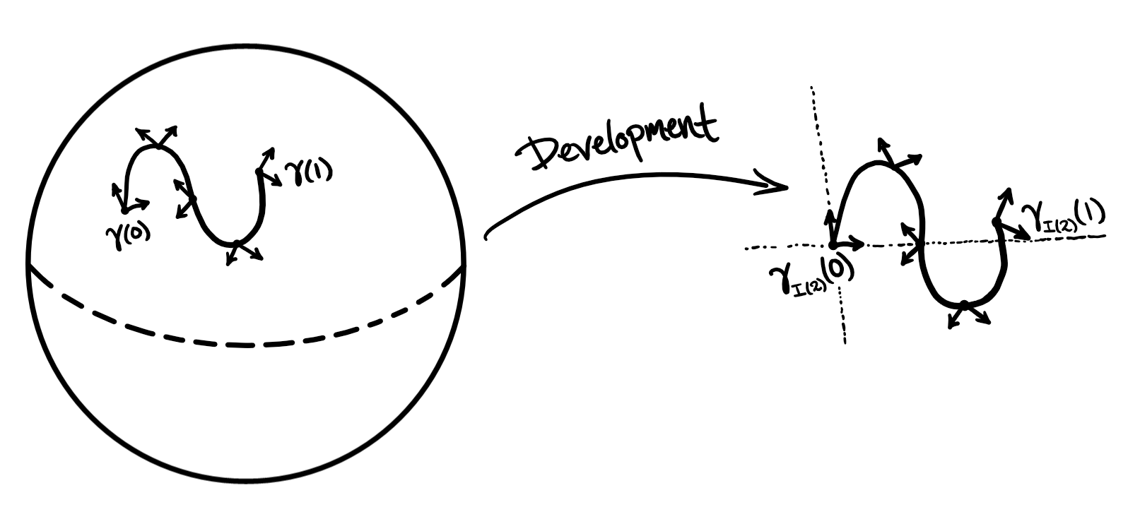
Intuitively, $\gamma$ gives us instructions for a path on ${G}$ in terms of our Cartan connection, and $\gamma_{{}_{G}}$ is the path we take if we try to follow these same instructions using the Maurer-Cartan form on $G$, starting at the identity. For example, if $\gamma$ is already a path on $G$, then $\gamma_{{}_{G}}$ is just the left-translate $\operatorname{L}_{\gamma(0)^{-1}}\circ\,\gamma$.

We now turn to the machinery described in [8]. Given a Cartan geometry $({G},\omega)$ of type $(G,H)$ over $M$, we can construct a principal $G$-bundle $\widehat{{G}}={G}\times_{H}G$ and a principal connection $\widehat{\omega}$ on $\widehat{{G}}$ that is characterized by $j^{*}\widehat{\omega}=\omega$, where $j:{G}\to\widehat{{G}},\penalty\ {g}\mapsto({g},e)$. This allows us to define an extrinsic notion of holonomy.

In [5] and [16], a more natural definition of holonomy was given, where the holonomy group was defined to be the subgroup of $G$ whose elements were developments along loops within the Cartan geometry. While this idea is on the right track, it has several issues that make it less viable than the extrinsic holonomy given above. For example, this alternative definition does not capture the orientation-reversing part of the holonomy of the locally Euclidean Klein bottle, since the corresponding loops on the Klein bottle do not lift to loops in the orthonormal frame bundle. In the next section, we will give a corrected version of this idea.

With holonomy in hand, we can define the notion of holonomy reduction used in [8].

This is called a holonomy reduction because, for $X=G/J$, it is equivalent to a reduction of structure group on $\widehat{{G}}$ from $G$ to $J$ such that $\widehat{\omega}$ pulls back to a principal $J$-connection under the corresponding inclusion, and the smallest choice of $J$ is the holonomy group. In other words, it is equivalent to a holonomy reduction of the extended principal bundle with the extended principal connection.

Of course, a section $\sigma$ of $\widehat{{G}}\times_{G}X$ is equivalent to a $G$-equivariant map $\sigma:\widehat{{G}}\to X$, and both are equivalent to an $H$-equivariant map $\sigma:{G}\to X$; we will follow the practice of not distinguishing between these maps.

We can now define curved orbits as collections of points whose fibers in ${G}$ have the same image under a holonomy reduction $\sigma$.

From this definition, it is not immediately apparent whether a curved orbit is anything more than a subset of $M$. Nevertheless, it was proved in [8] that each curved orbit is an initial submanifold of $M$, and that each of them carries a canonical geometric structure. Later, we will give an alternative perspective that makes this inherent structure obvious.

We begin with a corrected definition of holonomy.

Note that the holonomy of a loop $\gamma$ in the base manifold only depends on that loop and the chosen basepoint ${g}\in{G}$, since if $\widehat{\gamma}$ is our chosen lift starting at ${g}$, then every other lift starting at ${g}$ will be of the form $\operatorname{R}_{\beta}(\widehat{\gamma})$ for some path $\beta$ in $H$ starting at the identity, and $\operatorname{R}_{\beta}(\widehat{\gamma})_{{}_{G}}=\operatorname{R}_{\beta}(\widehat{\gamma}_{{}_{G}})$. Furthermore, this definition remains natural while still fixing the issues in the definitions given by [5] and [16]. Moreover, it is actually equivalent to the extrinsic holonomy.

The straightforwardness of this proof makes it particularly difficult for the author to believe that our small adjustment to the definition of holonomy used in [5] and [16] was not present in any of the previous literature that he could find. Nonetheless, while there are results in the literature¹¹ 1 See, for example, Proposition 2.1.1 of [5], which notes that the subgroups corresponding to holonomy from contractible loops coincide. that relate the extrinsic holonomy group to the holonomy group consisting of developments of closed loops in ${G}$ that lift from loops in $M$, our definition does not seem to have been considered before in the form presented above.

In a similar way, we can also simplify what we mean by a holonomy reduction.

Note that, if $\sigma^{-1}(eJ)$ is empty, then we can use a $g\in G$ such that $\sigma^{-1}(g^{-1}J)$ is not empty; the corresponding closed subgroup will change from $J$ to $g^{-1}Jg$.

It is well-known in the principal bundle context that a choice of closed subgroup $J$ containing the holonomy group determines a holonomy reduction, so the existence of a result like Proposition 3.3 is not particularly surprising. However, viewed through the heuristic analogy where we pretend $({G},\omega)$ is a Lie group, the idea that a holonomy reduction just amounts to specifying a basepoint and a particular closed subgroup takes on additional meaning. Indeed, if we pretend that ${e}$ is the “identity element” of $({G},\omega)$, then this allows us to specify a “subgroup” $\sigma^{-1}(eJ)$ of $({G},\omega)$, corresponding to $J\leq G$. In the next section, we will see that the “subgroup” $\sigma^{-1}(eJ)$ is an example of what we call a curved coset.

In this section, we will define curved cosets, describe some of their properties, and show how they are related to the curved orbits of [8]. To start, however, we need a way to compare elements of a Cartan geometry with elements in its corresponding model.

Unlike developments of paths, developments of points of ${G}$ are not necessarily unique. Indeed, suppose $\alpha:[0,1]\to{G}$ is a lift of a loop in $M$, so that $\alpha(0)={e}$ and $\alpha(1)={e}k$ for some $k\in H$. Then, if $\gamma:[0,1]\to{G}$ is a path with $\gamma(0)={e}$ and $\gamma(1)h={g}$ for some $h\in H$, then concatenating $\alpha$ with the right-translate $\operatorname{R}_{k}(\gamma)$ gives a path from ${e}$ to ${g}h^{-1}k$, so both $\gamma_{{}_{G}}(1)h$ and $\alpha_{{}_{G}}(1)(k^{-1}\gamma_{{}_{G}}(1)k)(h^{-1}k)^{-1}=(\alpha_{{}_{G}}(1)k^{-1})(\gamma_{{}_{G}}(1)h)$ are developments of ${g}$ from ${e}$. More succinctly, if $g$ is a development of ${g}$ from ${e}$, then so is every element of $\Hol_{e}({G},\omega)g$.

Thus, in the heuristic analogy between $({G},\omega)$ and $G$, if we think of ${e}$ as the “identity element”, then elements of ${G}$ correspond to elements of $G$, the elements of $G$ to which they correspond are given by their developments from ${e}$, and the holonomy group $\Hol_{e}({G},\omega)$ tells us exactly if and how this correspondence fails to assign a unique group element.

In the Klein geometry $(G,\omega_{{}_{G}})$ of type $(G,H)$, where the holonomy group is always trivial, the unique development of $g_{1}\in G$ from $g_{0}\in G$ is $g_{0}^{-1}g_{1}$, so the (left) coset $g_{0}J$ is precisely the set of all $g_{1}$ with development from $g_{0}$ contained in $J$. Analogously, we define curved (left) cosets of a Cartan geometry to be sets of points with developments contained in a given subgroup of $G$.

While the above definition works without the assumption that $J$ contains $\Hol_{g}({G},\omega)$, $\Hol_{g}({G},\omega)$ is the smallest sensible candidate for a choice of $J$, since by the considerations above, ${g}\bullet\{e\}={g}\bullet\Hol_{g}({G},\omega)$. Therefore, unless we indicate otherwise, we will assume that curved (left) cosets ${g}\bullet J$ are well-defined, meaning that $\Hol_{g}({G},\omega)\leq J$.

For a given ${g}\in{G}$, ${g}\bullet J$ being well-defined does not necessarily imply that ${g^{\prime}}\bullet J$ is well-defined for ${g}^{\prime}\not\in{g}\bullet J$. For $\gamma:[0,1]\to{G}$ a path starting at ${g}$ such that $\gamma(1)h^{\prime}={g}^{\prime}$, the curved coset ${g}^{\prime}\bullet J$ is well-defined if and only if $J$ contains $\Hol_{{g}^{\prime}}({G},\omega)=(\gamma_{{}_{G}}(1)h^{\prime})^{-1}\Hol_{g}({G},\omega)\gamma_{{}_{G}}(1)h^{\prime}$. In other words, ${g}^{\prime}\bullet J$ is well-defined for all ${g}^{\prime}\in{G}$ if and only if $\Hol_{g}({G},\omega)$ is contained in every subgroup that is conjugate to $J$ by an element of the form $\gamma_{{}_{G}}(1)h^{\prime}$. Because such conditions on the holonomy can be quite restrictive, we will also introduce a weaker notion of curved coset.

Similar to the above, we will say that ${g}\circ J$ is well-defined if and only if every path component of $J$ intersects $H$ and $\Omega^{\omega}_{{g}^{\prime}}(\mathfrak{j}\wedge\mathfrak{j})\subseteq\mathfrak{j}$ for all ${g^{\prime}}\in{g}\circ J$, where $\Omega^{\omega}$ is the curvature of $({G},\omega)$. Again, we could do without this assumption, but there is no real benefit to doing so: for $J^{\prime}$ the subgroup of $J$ generated by $J\cap H$ and the identity path component $J^{\circ}$, ${g}\circ J={g}\circ J^{\prime}$, and since $\Omega^{\omega}(X\wedge Y)=[X,Y]-\omega([\omega^{-1}(X),\omega^{-1}(Y)])$, the condition $\Omega^{\omega}_{{g}^{\prime}}(\mathfrak{j}\wedge\mathfrak{j})\subseteq\mathfrak{j}$ for all ${g}^{\prime}\in{g}\circ J$ just says that ${g}\circ J$ is a union of integral manifolds for the distribution $\omega^{-1}(\mathfrak{j})$. Thus, unless we indicate otherwise, we will assume that our geometric leaves are well-defined whenever we refer to them.

As an example, for every $K\leq H$, ${g}\circ K={g}K=\{{g}h:h\in K\}$ is always well-defined. Moreover, if we are working over the Klein geometry $(G,\omega_{{}_{G}})$, then the geometric leaf $g\circ J$ will be the coset $gJ^{\prime}$, where $J^{\prime}$ is the subgroup generated by the identity path component $J^{\circ}$ and $J\cap H$, so since we assume $g\circ J$ is well-defined, $J^{\prime}=J$ and $g\circ J=gJ=\{gj:j\in J\}$.

From their definitions, it is clear that ${g}\bullet J$ and ${g}\circ J$ are initial submanifolds of ${G}$ when they are well-defined and $J$ is a closed subgroup of $G$, and they inherit the structure of a Cartan geometry of type $(J,H\cap J)$ over the initial submanifolds $q_{{}_{H\cap J}}({g}\bullet J)$ and $q_{{}_{H\cap J}}({g}\circ J)$ of ${G}/(H\cap J)$, respectively, by pulling back by the inclusion map. Moreover, if ${g}h\in{g}\bullet J$ for some $h\in H$, then by definition developments of ${g}h$ from ${g}$ are contained in $J$, so $h\in H\cap J$. Thus, we can naturally identify $q_{{}_{H\cap J}}({g}\bullet J)$ with $q_{{}_{H}}({g}\bullet J)$.

We can actually say a bit more about the topology of ${g}\bullet J$.

If we fix a point ${e}\in{G}$ that we think of as the “identity element”, then both ${e}\bullet J$ and ${e}\circ J$ can reasonably be thought of as “subgroups” of $({G},\omega)$ when they are well-defined. Moreover, once we have chosen an “identity element” for $({G},\omega)$, we can assign developments from that point, and using this, we can define curved right cosets by analogy to $Jg=g(g^{-1}Jg)$.

Here, again, we might as well always require that $g^{-1}Jg$ contains $\Hol_{g}({G},\omega)$, since nothing is gained by assuming otherwise. However, since $\Hol_{e}({G},\omega)=g\Hol_{g}({G},\omega)g^{-1}$, this just means that $J$ has to contain the holonomy group at ${e}$, and if this holds, then curved right cosets through ${g}$ are well-defined independent of any condition on ${g}$.

Note that, in order to define these curved right cosets, we must choose a basepoint ${e}\in{G}$, so by Proposition 3.3, if $J$ is closed, then the data needed to define a curved right coset is precisely the data needed to define a holonomy reduction. In terms of the holonomy reduction $\sigma:{G}\to G/J$ induced by the choice of basepoint, if $g$ is a development of ${g}$, then

Moreover, $q_{{}_{H}}(J\bullet{g})=q_{{}_{H}}((J\bullet{g})H)=q_{{}_{H}}(\sigma^{-1}(Hg^{-1}J))$, and $q_{{}_{H}}(\sigma^{-1}(Hg^{-1}J))$ is the set of all points on the base manifold with $H$-type $Hg^{-1}J$, so curved orbits are just the projections of curved right cosets to the base manifold.

Interestingly, curved cosets are so well-behaved that we can even consider the corresponding quotient manifolds.

In particular, if $({G},\omega)$ is a Cartan geometry of type $(G,H)$, ${e}\in{G}$, and $J$ is a closed normal subgroup of $G$ containing $\Hol_{e}({G},\omega)$, then $J\backslash{G}$ is a principal $(H\cap J)\backslash H$-bundle and naturally inherits a Cartan connection $\bar{\omega}$ of type $(J\backslash G,(H\cap J)\backslash H)$ with trivial holonomy, given by $\pi_{{}_{J}}^{*}\bar{\omega}=\omega+\mathfrak{j}$.

When we want to study Lie groups, it is often useful to look at their representations. Naturally, then, when we want to study Cartan geometries, it might be useful to have a corresponding notion of representation. To that end, suppose we are given a Cartan geometry $({G},\omega)$ of type $(G,H)$ over a manifold $M$ and a finite-dimensional representation $\rho:G\to\GLin(V)$.

We would like to find a “representation” for $({G},\omega)$ corresponding to $\rho$. If we fix an “identity element” ${e}\in{G}$ and $\Hol_{e}({G},\omega)\leq\ker(\rho)$, then we have a convenient answer: define $\rho({g}):=\rho(g)$ for each ${g}\in{G}$, where $g\in G$ is some development of ${g}$ from ${e}$. Unfortunately, this is generally not a useful assumption to make for $({G},\omega)$; if $G$ is a connected centerless simple Lie group, for example, then the only normal subgroups of $G$ are $\{e\}$ and $G$ itself, so if $\Hol_{e}({G},\omega)$ is nontrivial, then this will only get us the trivial representation. Thus, while this is a good answer when it works, we would like something more general that does not have such stringent requirements on the holonomy.

Of course, the restriction $\rho|_{H}$ of $\rho$ to $H$ is still a representation. Thus, identifying $H$ with the “subgroup” ${e}\circ H={e}H$, we can try to form the “(co)induced representation” of $\rho|_{H}$ to $({G},\omega)$, given by the space $\Gamma({G}\times_{H}V)$ of sections of the associated bundle ${G}\times_{H}V$ over $M$, which we identify with the space of $H$-equivariant functions from ${G}$ to $V$. In the model case, $G$ acts on $\Gamma(G\times_{H}V)$ by $g\cdot\sigma:=\sigma\circ\operatorname{L}_{g^{-1}}$, and an isomorphic copy of the representation $\rho$ is contained in $\Gamma(G\times_{H}V)$, given by the subspace of sections of the form $\widetilde{v}:G\to V,g\mapsto\rho(g)^{-1}v$ with $v\in V$. This gives an identification of $G\times_{H}V$ with the trivial bundle $G/H\times V$, where the copy of $\rho$ in $\Gamma(G\times_{H}V)$ is precisely the subspace that is identified with the constant sections of $G/H\times V$.

In the general case, we lack a meaningful notion of action of $({G},\omega)$ on $\Gamma({G}\times_{H}V)$, and we do not necessarily have an isomorphism between ${G}\times_{H}V$ and $M\times V$. However, under the identification of $G/H\times V$ and $G\times_{H}V$ in the model case, the exterior derivative for $G/H\times V$ determines a corresponding differential operator $\nabla^{\rho}:\Gamma(G\times_{H}V)\to\Gamma(T^{\vee}(G/H)\otimes(G\times_{H}V))$ given by, for $X\in T(G/H)$ and $\sigma\in\Gamma(G\times_{H}V)$,

References

- [1] Alt, J.: Essential parabolic structures and their infinitesimal automorphisms. SIGMA Symmetry Integrability Geom. Methods Appl., vol. 7 (2011) arXiv:1011.0288v2
- [2] Armstrong, S.: Definite signature conformal holonomy: a complete classification. Journal of Geometry and Physics, vol. 57, issue 10, 2024-2048 (2007)
- [3] Armstrong, S.: Projective Holonomy I: Principles and Properties. (2007) arXiv:math/0602620v4
- [4] Armstrong, S.: Projective Holonomy II: Cones and Complete Classifications. (2007) arXiv:math/0602621v4
- [5] Baum, H., Juhl, A.: Conformal Differential Geometry: Q-curvature and Conformal Holonomy. Oberwolfach Seminars, vol. 40. Birkhäuser, Berlin (2010)
- [6] Blumenthal, R. A., Hebda, J. J.: The generalized Cartan-Ambrose-Hicks theorem. Geometriae Dedicata, vol. 29, 163-175 (1989)
- [7] Calderbank, D. M. J., Diemer, T.: Differential invariants and curved Bernstein-Gelfand-Gelfand sequences. J. reine angew. Math., issue 537, 67-103 (2001)
- [8] Čap, A., Gover, A. R., Hammerl, M.: Holonomy reductions of Cartan geometries and curved orbit decompositions. Duke Mathematical Journal, vol. 163, 1035-1070 (2014)
- [9] Čap, A., Slovák, J.: Parabolic Geometries I: Background and General Theory. Mathematical Surveys and Monographs, vol. 154. Amer. Math. Soc., Providence, RI (2009)
- [10] Čap, A., Slovák, J.: Weyl structures for parabolic geometries. Mathematica Scandinavica, vol. 93, no. 1, 53-90 (2003)
- [11] Čap, A., Slovák, J., Souček, V.: Bernstein-Gelfand-Gelfand sequences. Ann. of Math., vol. 154, no. 1, 97-113 (2001)
- [12] Frances, C.: Essential conformal structures in Riemannian and Lorentzian geometry, in Recent Developments in Pseudo-Riemannian Geometry. ESI Lectures in Mathematics and Physics, Eur. Math. Soc., Zürich, 231–260 (2008)
- [13] Frances, C.: Local dynamics of conformal vector fields. (2010) arXiv:0909.0044v2
- [14] Kobayashi, S., Nomizu, K.: Foundations of Differential Geometry. Interscience Tracts in Pure and Applied Mathematics, no. 15, vol 1, Wiley & Sons (1963)
- [15] McKay, B.: Complete Cartan connections on complex manifolds. (2005) arXiv:math/0409559v4
- [16] Sharpe, R. W.: Differential Geometry: Cartan’s Generalization of Klein’s Erlangen Program. Graduate Texts in Mathematics, vol. 166, Springer-Verlag, New York (1997)
- [17] Wu, H.: On the de Rham decomposition theorem. Illinois J. Math. vol. 8, no. 2, 291-311 (1964) https://projecteuclid.org/euclid.ijm/1256059674