An Efficient High-order Numerical Solver for Diffusion Equations with Strong AnisotropyJournal: Computer Physics Communications
Abstract
In this paper, we present an interior penalty discontinuous Galerkin finite element scheme for solving diffusion problems with strong anisotropy arising in magnetized plasmas for fusion applications. We demonstrate the accuracy produced by the high-order scheme and develop an efficient preconditioning technique to solve the corresponding linear system, which is robust to the mesh size and anisotropy of the problem. Several numerical tests are provided to validate the accuracy and efficiency of the proposed algorithm.
Keywords:
Anisotropic diffusion equation, Interior penalty discontinuous Galerkin, High-order method, Subspace correction methods, Iterative methods1 Introduction
Anisotropic diffusion is a common physical phenomenon and describes processes where the diffusion of some scalar quantity is direction dependent. In fusion plasmas diffusion tensors can be extremely anisotropic due to the high temperature and large magnetic field strength. For example, in plasma magnetic fusion devices, the electron heat conductivity along the magnetic field can be greater than that across the magnetic field by a factor of or even may reach the order of [39]. This anisotropy is due to the fact that the gryomotion of charged particles in a magnetic field results in slow transport perpendicular to the field while particles can travel comparatively long distances parallel to the field before undergoing a collision.
Strongly anisotropic diffusion problems present a numerical challenge, because errors in the direction parallel to the magnetic field may have significant effect on transport in the perpendicular direction. The widely used strategy to solve the anisotropic diffusion equations is to use finite-difference schemes with meshes aligned with the magnetic field direction. Flux aligned coordinates are used in the fusion community to obtain accurate diffusion simulations [11]. However, the generation of aligned meshes is still limited to comparably simple magnetic field topologies. For practical geometries, aligned mesh generation is still an open problem, particularly for fusion confinement devices with complicated magnetic topologies and plasma-facing component geometries. Alternative discretization schemes which do not rely on a magnetic field aligned grid have also been studied [30, 39], and such a discretization is the focus of this paper.
In order to relax the difficulties in generating the aligned mesh, there is increasing interest in non-aligned mesh schemes. These methods must overcome recognized difficulties arising for strongly anisotropic diffusion problems with non-aligned meshes, which include numerical perpendicular pollution, non-positivity, and loss of convergence [39]. Finite difference methods adopting interpolations aligned to the parallel diffusion direction have been proposed in [36]. Proper flux construction and high order finite difference schemes on the non-aligned meshes have been proposed in [17, 16]. Due to the flexibility in the geometry, the finite volume methods on the non-aligned meshes have also been investigated for example in [20] and the high order finite volume schemes has been studied in [7]. In the finite element community, the continuous linear finite element coupled with M-matrix adaption has been studied in [24]. Jardin [22] applies a finite element method with reduced quintic triangular finite elements where the quintic basis functions are constrained to enforce continuity across element boundaries.
Compared with other finite element methods, discontinuous Galerkin methods have many advantages, including flexibility in mesh generation, adopting hp-adaptive refinement, and preserving the essential conservation properties. Such methods have also been used to discretize the anisotropic diffusion operator by a discontinuous Galerkin scheme in [18] and a hybrid discontinuous Galerkin scheme in [14] for the non-aligned meshes. Both of these two approaches are able to achieve high order approximation by increasing the polynomial order which usually results in a similarly accurate solution with fewer total degrees of freedom than lower-order elements. In this paper, we shall also employ a high order scheme and additionally demonstrate the advantages in the interior penalty discontinuous Galerkin method. More details on the different types of discontinuous Galerkin methods can be found in [3].
However, the discontinuous Galerkin method will result in even a larger number of degrees of freedom than continuous finite element method and the computational cost can be higher due to the resulting ill-conditioned linear system. In fact, the condition number is even worse in the strong anisotropic diffusion case. As a result, an efficient implementation requires the use of advanced iterative methods for solving the resulting linear systems. Efficient solvers arising from the discontinuous Galerkin method can be found in [1] (Schwarz method), [10] (multilevel method) and [6] (multigrid methods). The subspace correction method [43] and auxiliary space preconditioning method [44] have also been used to construct an efficient linear solvers for the discontinuous Galerkin methods, see [8, 2]. In this paper, we will use the auxiliary space method to construct a robust preconditioner.
Our particular application focus for this paper is magnetized plasmas for fusion applications, where the scale separation induced by the magnetic field produces conduction coefficients that are several orders of magnitude larger in the parallel direction (denoted as ) than in the perpendicular direction (denoted as ). This work demonstrates that a high-order method is able to provide satisfactory numerical solutions on non-aligned meshes. We shall also construct an effective and robust preconditioner to solve the corresponding linear system. The remainder of this paper is organized as follows. Section 2 reviews the notation and proposes the numerical schemes for the anisotropic diffusion equations. The numerical experiments are reported in Section 3 to validate the accuracy tests for our proposed schemes. Then Section 4 and Section 5 are contributed to develop and verify the efficient linear solver and numerical tests for problems with strong anisotropy. The concluding remarks and future research plans will be discussed in Section 6.
2 Finite Element Spaces and Finite Element Schemes
In this section, we will review the notations in the continuous Galerkin (CG) and discontinuous Galerkin (DG) finite element scheme in the later sections. The DG methods will be used to discretize the given equations and the CG methods will be used in constructing the preconditioner.
2.1 Preliminaries
The problem under consideration is the following two-dimensional equation with anisotropic diffusivity. Let be a bounded connected domain in with Lipschitz boundary and let . We consider the following steady state anisotropic diffusion equation:
| (1) | |||||
| (2) |
where the diffusion coefficient tensor is given by
| (3) |
The direction of the anisotropy, or the magnetic field, is given by a unit vector . Here and represent the parallel and the perpendicular diffusion coefficient. Moreover, the anisotropy level is such that is several orders of magnitude larger than
Throughout this paper, the standard notations for Sobolev spaces will be adopted. For example, for a bounded domain , we denote by the standard Sobolev space of order with norm and semi-norms and respectively. If and/or , we shall omit and/or in the norm notations.
Partition: Denote a shape-regular partition of domain into two-dimensional simplices (triangles or quadrilaterals) as . Denote as the interfaces for all the elements with denoting the interior edges. Let , where denotes the diameter of element .
Trace Operators: For piecewise functions, we further introduce the jumps and averages as follows. For any edge , with as the outward unit normal to , the jumps of a scalar valued function across are defined as
and the averages of a scalar valued function is defined as
On the boundary , when , the jump and average operators are defined as , .
Continuous Finite Element Space: Let
| (4) |
where , , denotes the polynomials with degree less than or equal to .
Discontinuous Finite Element Space: Let
| (5) |
2.2 Continuous Galerkin Finite Element Method
In this section, we shall introduce the -finite element method (FEM). The -FEM is to find the numerical solution , such that
| (6) |
where the bilinear form
| (7) |
Remark 1
Well-posedness of CG for isotropic diffusion equations can be found in the many literatures, for example [5]. It is noted that the CG scheme can produce a symmetric positive definite linear system.
Remark 2
As with the traditional analysis for the isotropic diffusion equation, we can expect the optimal convergence rate for -error at the order if . However, in the strong anisotropic case, the optimal rate of convergence is usually hard to obtain with low order schemes due to spurious numerical diffusion. Some benchmark tests can be found in [19].
Remark 3
The following condition number estimation result for two dimensional anisotropic diffusion equations discretized by the linear CG method can be found in [23]. The condition number of the stiffness matrix for is bounded by
Here denotes a constant, denotes the minimum eigenvalue of on , denotes the number of elements, is the element patch associated with the th vertex, is the average of over , is the Jacobian matrix of the affine mapping from the reference element to the physical element , and denotes the average element size. In this conditioning estimate, the first factor corresponds to the condition number of the stiffness matrix for the Laplacian operator. The second factor reflects the effects of the volume weighted, combined alignment and equidistribution quality measure of the mesh with respect to anisotropic diffusion tensor . The third term measures the mesh volume-nonuniformity. We also note that there are many references (e.g., [24, 21, 25]) developing the anisotropy-adaptive (-adaptive) meshing techniques in the continuous linear finite element framework. However, it is not a focus for this paper.
2.3 Discontinuous Galerkin Finite Element Method
Now, we are ready to introduce the numerical algorithm for solving anisotropic diffusion equation by using piecewise polynomials without any continuous constraints. The interior penalty discontinuous Galerkin (IPDG) numerical algorithm is to find such that
| (8) |
where
If , we obtain the symmetric IPDG scheme and , we obtain the non-symmetric IPDG scheme. The parameter has to be chosen to ensure stability.
Remark 4
The well-posedness of DG can be found in [41]. Briefly speaking, in the case of symmetric IPDG scheme, the penalty parameter is required to be large enough to ensure stability; however, in the case of non-symmetric IPDG scheme, we only need the penalty parameter to be positive.
Remark 5
For two-dimensional simulation, the penalty parameter for symmetric IPDG schemes with is widely chosen as
In the remainder of this paper, we shall only focus on the symmetric IPDG scheme with the penalty parameter below,
| (9) |
In the above parameter setting, is weighted with the nodal distance in each element and is based on the modulation of the stabilization with respect to the actual strength of the parallel diffusion in the normal direction of each face.
Remark 6
Let , where indicates the maximum eigenvalue of on . Let denotes the minimum eigenvalue of on . Suppose and the numerical scheme is wellposed, then the following error estimate [12] holds,
| (10) |
The above inequality also demonstrates that in the case of strong anisotropy, there may be large numerical pollution in the low order schemes due to the term.
3 Numerical Experiments for Testing Accuracy
In this section, we first study the accuracy of the above IPDG numerical schemes. We demonstrating that:
- 1.
The simulation on the aligned meshes can resolve the anisotropy to some level and is able to provide the satisfactory numerical solutions.
- 2.
The high-order IPDG schemes on the un-aligned meshes are still able to produce reliable numerical simulations.
Errors are measured in -norm to validate our results, with the optimal rates in convergence being at the order , where denotes the polynomial degree in the IPDG scheme.
3.1 Aligned Mesh
In this section we demonstrate the IPDG scheme on a series of aligned meshes of increasing resolution for three problems of increasing solution variability in the perpendicular direction. Section 3.2 examines the scheme’s performance for the non-aligned meshes.
3.1.1 Test: Error versus for varying mesh and penalty parameters
 |
 |
 |
| (a) | (b) | (c) |
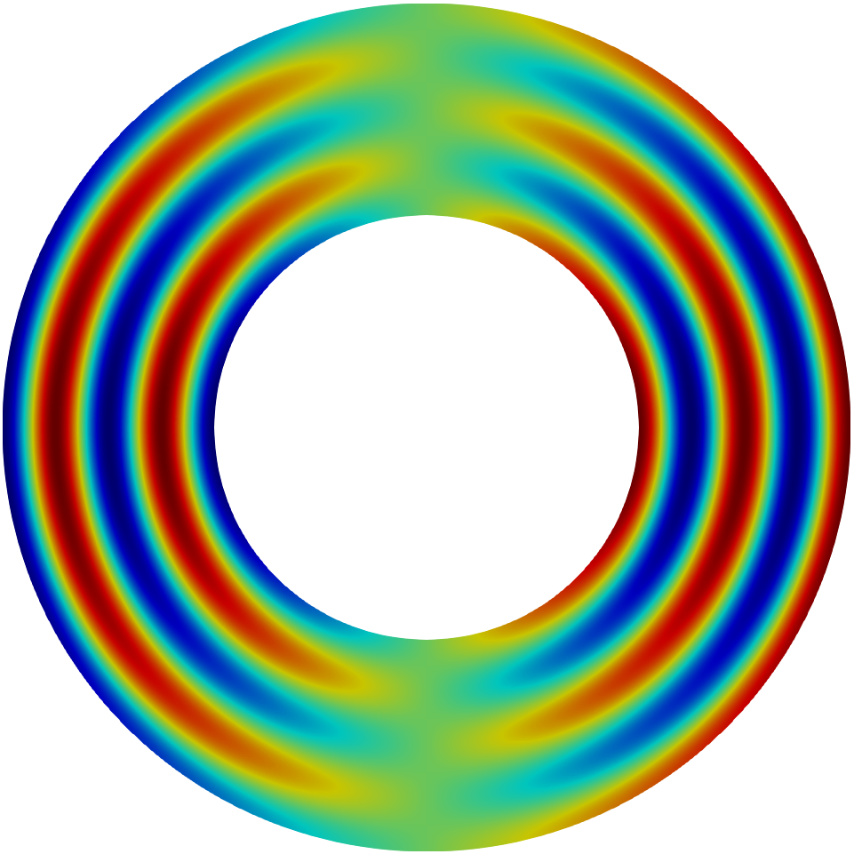
Problem Setting: In this test, the computational domain is an annulus with exterior radius and interior radius , and the magnetic field direction is circular with the following expression
| (11) |
The diffusion tensor (3) is set with and varying values of . Here, is the frequency of oscillation in the perpendicular direction.
The manufactured solutions are plotted in Figure 1 for and the discretizations are based on the quadrilateral meshes shown in Figure 2. For , we utilize the mesh with (Figure 2a); for , (Figure 2b); and for , (Figure 2c).
 |
 |
 |
| (a) | (b) | (c) |
The numerical performance for on the Mesh with (Figure 2a) is summarized in Figure 3. The corresponding linear system is solved directly with package “sparsecholesky" [15]. The 1D plots show the values of the -error for varying between and . With both penalty parameters and , the value of the -error remains constant whatever the value of , except for where it finishes by increasing at large values (). This behavior has to be related to the constant increase of the condition number of the matrix with when solving the linear system with a direct solver. As long as the anisotropy remains moderate in our test case, the -error remains dominated by the polynomial interpolation errors. However, in the case with strong anisotropy, the error from the linear solver dominates over the interpolation error, and thus leads to an increase of the -error. The error behavior in the high-order scheme may be solved by employing other direct solvers. For either value of (), the behavior is very similar when comparing the -error. For simplicity, we shall choose the penalty parameter in all of the following tests.
 |
 |
| (a) | (b) |
Next, we shall test the performance for and with . Since our direct solver can handle the condition numbers in these linear systems, we can expect flat behavior in the error with . Because of the increase in perpendicular frequency we partition the domain with more divisions in the radial direction as shown in Figure 2a-b. The -errors with respect to the values in are plotted in Figure 4. Again, we obtain the expected performance that the -errors remain almost constant with and thus validate our stabilization conclusions in the parameter .


3.2 Non-Aligned Mesh
In this section, we shall demonstrate the performance of the high-order scheme on the non-aligned mesh and show that satisfactory numerical solutions can be obtained.
3.2.1 Test: Constant magnetic field
 |
 |
| (a) | (b) |
Problem Setting: The computational domain is chosen as , with a Dirichlet boundary condition at the vertical boundary , where the solution is imposed. The rest of the boundaries are with homogeneous Neumann conditions. The magnetic field is vertical with components and . The perpendicular diffusion is set as , and a source is imposed with the form
The analytical solution is . Since the value of the parallel diffusion does not affect the analytical solution, the effect on the numerical solution is entirely due to the numerical diffusion introduced by the scheme on a given discretization. Results from the aligned quadrilateral mesh (Figure 5a) and non-aligned triangular mesh (Figure 5b) are compared below.
 |
 |
| (a) | (b) |
We plot the numerical solution on the trace and compare it with the analytical solution in Figure 6. For the isotropic case with , the linear () solutions on the non-aligned and aligned meshes agree with the analytical solution. In the strongly anisotropic case with , the linear () numerical solution on the aligned mesh matches the exact solution. However, the low order numerical schemes on the non-aligned triangular mesh () produce polluted numerical solutions. As we increase the polynomial degree up to , the numerical solution on the non-aligned triangular mesh matches the analytical solution. Thus, when the aligned mesh challenging to generate or use in a simulation, we may need to adopt high-order computational scheme to obtain satisfactory numerical solutions.
3.2.2 Test: Diffusion of a Gaussian Source
 |
 |
| (a) | (b) |
Problem Setting: Let the computational domain be an annulus with exterior radius and interior radius . In this test, a Gaussian source is diffused towards an identical sink. The source and sink are defined as
where and . The magnetic field direction is chosen as . In this test, we shall choose and .
The source is plotted in Figure 7a. The numerical solution for , on the quadrilateral aligned mesh is shown in Figure 7b.
Since , the solution is expected to be diffused only in the parallel direction. This means that the normalized profiles (with respect to the maximum on each radial line) should overlap the plot of . Therefore, the difference between normalized profiles and the expected profile is from the error introduced via polluted numerical diffusion. In Figure: 8 we show the trace plot along the four lines illustrated in Figure 7b calculated using the quadrilateral aligned mesh for the angles . For all the trace locations, the figures show that the aligned discretizations provide satisfied solutions at any polynomial degree .
 |
 |
 |
| (a) | (b) | (c) |
 |
 |
 |
| (a) | (b) | (c) |
However, Figure 9 shows that the non-aligned triangular mesh does not behave well when the scheme order is low. As we can see from this figure, a significant spreading of the solution is visible for the low order elements ( and ) but for high-order elements a satisfactory numerical solution is obtained. Again, it suggests we adopt a high-order scheme for the non-aligned mesh.
3.2.3 Test: Two Magnetic Islands
 | |
| (a) | (b) |
Problem Setting: Let the computational domain be and the exact solution be
| (12) |
Let and
| (13) |
The perpendicular diffusion is set as with varying values of for the diffusion tensor (3). The magnetic field and the exact solution are plotted in Figure 10. It is noted that the magnetic field shows two islands.
Due to the complexity of the magnetic direction, it is almost impossible to generate an aligned mesh for resolving the problem’s anisotropy. Here we shall investigate the performance of the high order scheme on the Cartesian grid with partitions in both and directions.
| = 1E1 | = 1E2 | = 1E4 | = 1E6 | = 1E8 | ||||||
|---|---|---|---|---|---|---|---|---|---|---|
| order | order | order | order | order | ||||||
| 8 | 2.44E-02 | 5.54E-02 | 7.12E-02 | 7.14E-02 | 7.14E-02 | |||||
| 16 | 8.31E-03 | 1.56 | 3.26E-02 | 0.77 | 5.66E-02 | 0.33 | 5.70E-02 | 0.33 | 5.70E-02 | 0.33 |
| 32 | 2.39E-03 | 1.80 | 1.40E-02 | 1.22 | 4.73E-02 | 0.26 | 4.85E-02 | 0.23 | 4.85E-02 | 0.23 |
| 64 | 6.33E-04 | 1.92 | 4.50E-03 | 1.64 | 3.90E-02 | 0.28 | 4.27E-02 | 0.18 | 4.28E-02 | 0.18 |
| 128 | 1.62E-04 | 1.97 | 1.24E-03 | 1.86 | 2.84E-02 | 0.46 | 3.86E-02 | 0.15 | 3.87E-02 | 0.14 |
| 256 | 4.10E-05 | 1.99 | 3.23E-04 | 1.94 | 1.51E-02 | 0.91 | 3.54E-02 | 0.12 | 3.59E-02 | 0.11 |
| 4 | 5.68E-03 | 1.20E-02 | 1.73E-02 | 1.74E-02 | 1.74E-02 | |||||
| 8 | 6.01E-04 | 3.24 | 1.36E-03 | 3.14 | 7.80E-03 | 1.15 | 8.26E-03 | 1.08 | 8.26E-03 | 1.07 |
| 16 | 7.16E-05 | 3.07 | 1.22E-04 | 3.49 | 3.22E-03 | 1.28 | 4.91E-03 | 0.75 | 4.94E-03 | 0.74 |
| 32 | 8.84E-06 | 3.02 | 1.11E-05 | 3.45 | 4.93E-04 | 2.71 | 3.35E-03 | 0.55 | 3.56E-03 | 0.47 |
| 64 | 1.10E-06 | 3.00 | 1.19E-06 | 3.23 | 3.67E-05 | 3.75 | 1.56E-03 | 1.11 | 2.85E-03 | 0.32 |
| 128 | 1.38E-07 | 3.00 | 1.40E-07 | 3.08 | 2.42E-06 | 3.92 | 1.95E-04 | 3.00 | 2.23E-03 | 0.35 |
| 4 | 7.04E-04 | 1.15E-03 | 6.65E-03 | 7.34E-03 | 7.35E-03 | |||||
| 8 | 4.48E-05 | 3.98 | 6.43E-05 | 4.16 | 5.26E-04 | 3.66 | 9.12E-04 | 3.01 | 9.41E-04 | 2.96 |
| 16 | 2.78E-06 | 4.01 | 3.16E-06 | 4.35 | 5.17E-05 | 3.35 | 1.05E-03 | -0.21 | 1.33E-03 | -0.50 |
| 32 | 1.74E-07 | 4.00 | 1.80E-07 | 4.13 | 1.36E-06 | 5.25 | 8.98E-05 | 3.55 | 8.84E-04 | 0.59 |
| 64 | 1.09E-08 | 4.00 | 1.10E-08 | 4.03 | 3.79E-08 | 5.16 | 2.32E-06 | 5.27 | 1.32E-04 | 2.74 |
| 128 | 6.83E-10 | 4.00 | 6.83E-10 | 4.01 | 1.25E-09 | 4.92 | 6.45E-08 | 5.17 | 3.37E-06 | 5.29 |
| 4 | 3.64E-05 | 5.19E-05 | 9.96E-04 | 3.08E-03 | 3.14E-03 | |||||
| 8 | 1.03E-06 | 5.15 | 1.50E-06 | 5.11 | 1.70E-05 | 5.88 | 9.21E-05 | 5.06 | 9.92E-05 | 4.99 |
| 16 | 3.04E-08 | 5.08 | 3.76E-08 | 5.32 | 1.34E-07 | 6.99 | 1.31E-06 | 6.14 | 8.19E-06 | 3.60 |
| 32 | 9.16E-10 | 5.05 | 1.02E-09 | 5.20 | 2.45E-09 | 5.77 | 9.02E-09 | 7.18 | 5.38E-07 | 3.93 |
| 64 | 2.81E-11 | 5.03 | 2.96E-11 | 5.11 | 5.56E-11 | 5.46 | 4.43E-10 | 4.35 | 6.52E-08 | 3.04 |
| 2 | 2.62E-04 | 3.71E-04 | 4.12E-03 | 5.22E-03 | 5.23E-03 | |||||
| 4 | 3.12E-06 | 6.39 | 4.81E-06 | 6.27 | 9.10E-05 | 5.50 | 3.43E-04 | 3.93 | 3.53E-04 | 3.89 |
| 8 | 7.58E-08 | 5.36 | 8.81E-08 | 5.77 | 5.14E-07 | 7.47 | 1.59E-05 | 4.43 | 9.97E-05 | 1.82 |
| 16 | 1.09E-09 | 6.12 | 1.14E-09 | 6.27 | 5.62E-09 | 6.52 | 9.92E-08 | 7.32 | 2.01E-06 | 5.63 |
| 32 | 1.66E-11 | 6.03 | 1.68E-11 | 6.09 | 3.92E-11 | 7.16 | 4.08E-10 | 7.93 | 1.42E-08 | 7.15 |
| 1 | 1.50E-03 | 3.18E-03 | 2.83E-02 | 5.24E-02 | 5.29E-02 | |||||
| 2 | 1.70E-05 | 6.46 | 3.72E-05 | 6.42 | 7.55E-04 | 5.23 | 1.35E-03 | 5.28 | 1.36E-03 | 5.28 |
| 4 | 3.18E-07 | 5.74 | 5.40E-07 | 6.11 | 5.49E-06 | 7.10 | 1.10E-04 | 3.61 | 1.73E-04 | 2.97 |
| 8 | 1.91E-09 | 7.38 | 2.67E-09 | 7.66 | 2.84E-08 | 7.60 | 5.60E-07 | 7.62 | 9.63E-06 | 4.17 |
| 16 | 1.37E-11 | 7.12 | 1.63E-11 | 7.36 | 7.90E-11 | 8.49 | 2.53E-09 | 7.79 | 1.57E-08 | 9.26 |
Table 1 shows the error profiles and the convergence results for varying values of and polynomial degrees by using the uniform rectangular meshes. It shows that with small anisotropy (1 and 1E2), the scheme can still produce the optimal rate of convergence, which is at the order . As expected, increasing the values of also increases the -error. However, for low order schemes (1 and 2) we do not observe the correct convergence rates. When the mesh is fine enough, the use of cubic elements is able to produce satisfactory numerical solutions with the numerical errors at the order below . In addition, one can observe that by increasing the polynomials’ degree further, we obtain the desired numerical results with the extreme anisotropic ratios .
3.3 Test: Convergence Test for Aligned and Non-aligned Meshes
 |
 |
| (a) | (b) |
In this test, we shall choose the manufactured solutions in (11) to test the numerical performance on the aligned quadrilateral mesh and non-aligned triangular meshes (as illustrated in Figure 11).
Results are shown in Figure 12 and Figure 13 for an isotropic case () and an anisotropic case (), respectively. We summarize our conclusions as below.
| (a) | (b) |
For the isotropic case (Figure 12), the convergence of -error is nearly independent of the features of the mesh. The theoretical convergence rate is achieved for all the polynomial approximations.
| (a) | (b) |
For the strongly anisotropic case, the convergence results of the -error depends on the nature of the mesh type for low order elements. In the aligned quadrilateral mesh, the optimal rate of convergence can still be obtained, as indicated by the slope plots in Figure 13a. In the triangular mesh, by using linear elements, we barely observe any convergence order with respect to mesh size . In the case of quadratic elements, we can can obtain second order convergence but it should be third order. When the polynomial’s degree is increased up to and , the correct convergence results are recovered by the simulation. As such, the general conclusion of this section is that as we increase the polynomial degree, the impact on the non-alignment of the mesh is reduced and we recover the expected convergence behavior.
3.4 Conditioning of the Corresponding Linear System
This sub-section is contributed to investigate the conditioning results of the derived IPDG schemes in the strong anisotropy cases. The problem setting is chosen the same as Test 3.1.1. In the following, we shall demonstrate the performance (in terms of condition number) of the aligned and non-aligned meshes.
| (a) | (b) |
In Figure 14 we test the performance on the quadrilateral and triangular meshes (from Figure 11) in the condition number sense for accuracy. The performance is very similar for both mesh types. The computed condition numbers (computed by the command “condest" in PyAMG). It is noted that the conditional number is increasing almost at the order of except when where it appears bounded as we keep increasing the values in . We are still not clear about this phenomenon and will leave it for interested readers to investigate. Thus in the scheme with , the derived linear systems may have extremely large condition numbers in the strong anisotropic diffusion case. In such cases, an effective preconditioner is needed for an accurate and efficient numerical solver.
4 Auxiliary Space Preconditioners
In this section, we introduce auxiliary space preconditioners (ASP) [29, 44] for solving the IPDG discretization (8). The IPDG method (8) can be written in the following operator form: given , find such that
where is the dual of and is the operator corresponding to the bilinear form . In order to design preconditioners using the auxiliary space preconditioning framework, as suggested in [2], we consider the following product of auxiliary spaces:
Note that, since , this product of the auxiliary spaces can also be considered as a special subspace decomposition of , i.e., . Naturally, is endowed with inner product whose operator form is with being the dual of . In addition, the transfor operator is the natrual inclusion in this case and its transpose, , is the usual projection.
Now, we can introduce the auxiliary space preconditioner, , as follows,
| (14) |
where the operator is the so-called smoother operator, which usually handles the oscillatory high frequency components in . In this work, we simply use the Jacobi smoother. Other smoothers, such as the Gauss-Seidel method, could be used here as well.
As we can see, to implement the preconditioner (14) in practice, we need to invert exactly. However, this might be challenging or even impractical when the problem size is large, polynomal degree is high, and/or the anisotropicity is strong. Therefore, in practice, we usually replace by a robust preconditioner and , i.e., we solve the auxiliary problem in approximately. This results in the following inexact version auxiliary space preconditioner,
Next we discuss our choices of . Notice that is the linear system obtained by using -FEM for solving the anisotropic diffusion equation (1)-(2). When , i.e., the linear FEM method, it is well-known that tailored multigrid (MG) methods and their algebriac variants, algebraic multigrid (AMG) methods, can be used [26, 28, 34, 13, 35, 4, 42, 45]. Therefore, we use when . In general, many existing efficient solvers for solving anisotropic diffusion problem discretized using linear elements can be applied here.
For high-order elements, i.e. , we again use auxiliary space preconditioning framework to develop an efficient solver by considering the following product of auxiliary spaces for ,
where is the linear finite element space, i.e., with . Since , this again can be considered as a subspace decomposition . The transfer operator here is just the inclusion and its transpose is the usual projection . To solve the auxiliary problem in , i.e., with , as we discussed before, we simply apply MG methods . Therefore, the overall auxiliary space preconditioner can be defined as where denotes some smoother in which we will discus later. Overall, the choice of in our implementation is
Since we are dealing with anisotropic problems and high-order elements are used, the choice of the smoother is crucial to achieve a good performance. As suggested in [31, 32, 2], when using high-order to solve isotropic problems, Schwarz-type block smoothers should be used and the blocks should be the blocks corresponding to the vertex patchs. On the other hand, for anisotropic problems, line smoothers should be applied when the standard coarsening strategy is used in the MG methods [42, 45, 37, 33]. Therefore, we use Schwarz-type block line smoothers as and each block includes all the elements sharing vertices along a line, which is usually orthogonal to the anisotropic direction.
To summarize, the inexact version auxiliary space preconditioner is
| (15) |
We will specify our implementations of , , and for the test problems in the numerical experiments later.
5 Numerical Experiment for Testing the Preconditioners
 |
|
| (a) | (b) |
Problem Setting. Test 5. In this test, let the computational domain be an annulus with exterior radius and interior radius . We shall choose the annulus test with following exact solution, diffusion coefficient, and external source as
The exact solution and the magnetic field are plotted in Figure 15. The diffusion tensor is of the form (3). We shall test the numerical performance with varying values in and . In the following, we shall demonstrate
- 1.
The high order scheme has an advantage in the both degrees of freedom and conditioning.
- 2.
5.1 Examination of conditioning of the high order schemes for fixed accuracy
 |
 |
 |
| (a) | (b) | (c) |
While in Section 3.4 it was seen that the condition number of the resulting linear system increases with scheme order, that test did not hold the accuracy constant and so the as the order was increased, so was the accuracy. In this section we examine the condition number (ConNum) while holding the accuracy as measured by -error (L2Err) approximately constant, and additionally compare the required degrees of freedom (DoFs). Figure 16 plots the absolute errors on different meshes with varying polynomial degrees for the anisotropic ratio 1E6. We observe that for linear DG elements, and in order to obtain the -errorE-2, a very fine mesh with and is required. The DoFs of the corresponding linear system are around E7. By using quadratic polynomials, we only need and , which requires DoFsE5 to achieve a similar -error. As we increase the degree to , there is a reductions in DoFs to achieve similar accuracy. Examining the condition numbers, we observe a significant reduction from 5.3E4 for linear elements, to 2.3E4 for quadratic elements, and to 8.0E3 for cubic elements. This suggests that employing high-order methods not only obtains the required accuracy, but also achieves significant computational savings.
5.2 Performance of the preconditioner
In this section we perform three tests to demonstrate the performance of our proposed preconditioner. In Sec. 5.2.1 we use different meshes with varying values in anisotropy to examine the preconditioner performance using applied to the linear finite element problem and solving system exactly; in Sec. 5.2.2 we look at performance as a function of scheme order, but still using to give an exact solution to the system; and finally in Sec. 5.2.3 we present preconditioner performance for varying order while using to solve the system approximately. In all three cases, our proposed preconditioner is effective.
| Cond() | PCG Iter() | Cond() | CG Iter() | |
| 1 | 1.93E+01 | 19 | 6.92E+02 | 129 |
| 1E+2 | 3.33E+01 | 28 | 1.95E+04 | 596 |
| 1E+4 | 3.28E+01 | 32 | 4.16E+04 | 1411 |
| 1E+6 | 3.35E+01 | 33 | 4.80E+04 | 1453 |
| 1E+8 | 3.30E+01 | 33 | 4.46E+04 | 1375 |
| 1E+10 | 3.37E+01 | 36 | 4.29E+04 | 1289 |
| 1 | 2.16E+01 | 17 | 2.66E+03 | 215 |
| 1E+2 | 3.50E+01 | 26 | 2.66E+04 | 1152 |
| 1E+4 | 3.41E+01 | 33 | 4.85E+04 | 4922 |
| 1E+6 | 3.81E+01 | 35 | 4.87E+04 | 5000+ |
| 1E+8 | 3.79E+01 | 35 | 5.39E+04 | 5000+ |
| 1E+10 | 3.72E+01 | 35 | 4.74E+04 | 5000+ |
| 1 | 2.28E+01 | 25 | 7.19E+03 | 336 |
| 1E+2 | 3.44E+01 | 37 | 3.66E+04 | 1965 |
| 1E+4 | 3.76E+01 | 40 | 5.11E+04 | 5000+ |
| 1E+6 | 4.11E+01 | 39 | 5.14E+04 | 5000+ |
| 1E+8 | 4.19E+01 | 41 | 5.14E+04 | 5000+ |
| 1E+10 | 4.40E+01 | 42 | 5.14E+04 | 5000+ |
5.2.1 Conditioning Results for Linear Finite Elements
Here we demonstrate the effectiveness of our proposed preconditioner for linear finite elements with varying mesh size spanning with . The conditioning results are reported in Table 2. The condition numbers are again computed by the command “condest” in PyAMG and the conjugate gradient (CG) method with stopping criterion (1E-6) has been applied for validating the effectiveness of our preconditioner. Here, we use Jacobi method for and, for the -problem, the action of in (14) is obtained by adopting the direct solver. The results show that the condition number for the stiffness matrix is related to the mesh size and the value of . When refining the mesh, the condition number usually increases at about . However, the results show that the condition number from a fixed mesh with increasing values in is bounded by the order . We do not know the reason for this behaviour. In contrast to the results for original stiffness matrix, the pre-conditioned system has a bounded condition number, which is around . When the CG iterative solver is applied to solve the problem, the pre-conditioned system needs around 40 iterations to achieve the required accuracy 1E-6. We observe that the iteration numbers for CG (with tol = 1E-6) for the preconditioned system are almost independent with the values in and . However, the required iteration numbers in the CG for the original linear system are significantly larger where when the mesh is finer or the value in is large, the CG solver fails to converge within 5000 iterations. This validates the efficiency and effectiveness of our proposed preconditioner.
5.2.2 Solve problem exactly for varying scheme order: .
For varying degree of the numerical schemes, here we test the performance of (14) where the -problem, is solved exactly via a direct solver. In addition, we use the Jacobi method for . The numerical results are shown in Table 3 and Table 5 for two different mesh sizes. We used the generalized minimal residual method (GMRES) with stopping tolerance 1E-6 to solve the pre-conditioned system in order to achieve more robust performance since in practice the linear system becomes ill-conditioned and CG may suffer loss of orthogonality due to numerical instability. As shown in these two tables, the required number of iterations is almost constant and independent of polynomial degree , values of , or the mesh size . The convergence results for the relative residual in the iterative solver for are plotted in Figure 17a and Figure 18a. The reduction rates in this plot is at the rate . Therefore, our results demonstrate that the -problem can provide an effective and robust preconditioner which controls the condition number in the DG system. However, in the cases of finer mesh size, high order schemes, and/or extreme anisotropy, the direct solver for the corresponding -problem may still be infeasible. Hence, the inexact version , in which the same -problem is solved approximately, is adopted below.
5.2.3 Solve problem inexactly for varying scheme order: .
In our implementation of , we again use the Jacobi method for . We use the smoothed aggregation AMG method for when solving the auxiliary problem in the linear finite element space as suggested in [35]. As we discussed, should be a Schwarz-type block line smoother. To be more precise, for this test problem, and since the computational domain is an annulus and the anisotropicity is along the circular direction, the blocks for the line smoother should be constructed along the radial direction. In practice, we first find the vertices along each radial direction on the mesh and then use all the unknowns (which can be found by looking at the nonzeros in the stiffness matrix ) that are connected to those vertices to form line blocks along the radial direction. We refer to the block line smoother using those blocks as . In addition, due to the fact the domain is an annulus, our test problem is periodic in the circular direction which leads to extra high-frequency components along the circular direction. Therefore, we also use block line smoothers along the circular direction. The line smoother in the circular direction is more precisely described by the following procedure: we find the vertices along each circular direction on the mesh and use all the unknowns (which, again, can be found by looking at the nonzeros in ) that are connected to those vertices to form line blocks along the circular direction. We refer to the block line smoother using those blocks as . Overall, we use and in a multiplicative fashion to define , i.e., . In addition, to further improve the robustness of the preconditioner, we use as a preconditioner for GMRES to solve inexactly with a tolerance of and switch the outer Krylov method for solving to a flexible version of GMRES with a tolerance of . The numerical results are presented in Table 4 and 6 for mesh size of and , respectively. As we can see, the number of iterations roughly stay the same for the different polynomials degrees and anisotropic diffusion coefficient . In addition, since we solve the auxiliary problem inexactly, the Krylov method takes slightly more iterations to converge than when the problem is solved exactly, which is expected. The convergence results for the relative residual of the iterative solve for are plotted in Figure 17b and Figure 18b. Overall, the numerical results demonstrate that the inexact preconditioner is robust and effective for this test problem.
| 1 | 23 | 27 | 22 | 24 | 23 | 28 | 26 | 30 |
|---|---|---|---|---|---|---|---|---|
| 1E+2 | 39 | 47 | 39 | 40 | 34 | 38 | 37 | 42 |
| 1E+4 | 47 | 64 | 52 | 55 | 51 | 53 | 54 | 56 |
| 1E+6 | 46 | 73 | 56 | 58 | 53 | 54 | 55 | 56 |
| 1E+8 | 39 | 62 | 59 | 58 | 53 | 54 | 55 | 56 |
| 1E+10 | 35 | 59 | 52 | 54 | 53 | 54 | 55 | 56 |
| 1 | 25 | 27 | 23 | 25 | 27 | 30 | 32 | 35 |
|---|---|---|---|---|---|---|---|---|
| 1E+2 | 39 | 47 | 39 | 40 | 38 | 43 | 46 | 49 |
| 1E+4 | 47 | 64 | 53 | 56 | 53 | 57 | 60 | 62 |
| 1E+6 | 46 | 73 | 57 | 58 | 54 | 54 | 55 | 57 |
| 1E+8 | 39 | 62 | 63 | 58 | 53 | 54 | 55 | 56 |
| 1E+10 | 35 | 59 | 56 | 60 | 60 | 54 | 55 | 56 |
| (a) | (b) |
| 1 | 22 | 26 | 20 | 23 | 21 | 25 | 22 | 27 |
|---|---|---|---|---|---|---|---|---|
| 1E+2 | 40 | 48 | 35 | 35 | 27 | 36 | 29 | 37 |
| 1E+4 | 52 | 64 | 49 | 51 | 42 | 45 | 47 | 50 |
| 1E+6 | 54 | 109 | 60 | 62 | 53 | 55 | 55 | 57 |
| 1E+8 | 53 | 90 | 60 | 62 | 53 | 55 | 55 | 56 |
| 1E+10 | 43 | 80 | 75 | 62 | 53 | 55 | 55 | 56 |
| 1 | 22 | 26 | 23 | 25 | 28 | 31 | 33 | 35 |
|---|---|---|---|---|---|---|---|---|
| 1E+2 | 40 | 48 | 35 | 36 | 35 | 40 | 41 | 45 |
| 1E+4 | 52 | 64 | 50 | 52 | 50 | 61 | 65 | 69 |
| 1E+6 | 54 | 109 | 60 | 63 | 61 | 58 | 58 | 62 |
| 1E+8 | 53 | 90 | 65 | 63 | 57 | 60 | 64 | 64 |
| 1E+10 | 43 | 80 | 80 | 80 | 61 | 69 | 69 | 69 |
| (a) | (b) |
6 Conclusions
In this paper, an interior penalty discontinuous Galerkin finite element scheme has been presented for the discretization of diffusion equations with strong anisotropy. With a high order scheme, the method is potentially able to discretize problems of relevance to magnetized plasma physics where complex magnetic topologies and plasma-facing component geometries (which describe the domain boundary) make the generation of magnetic field aligned meshes difficult or impossible. The preconditioner, constructed by the -problem together with the Jacobi smoother, has been demonstrated to solve the corresponding linear systems efficiently. Future applications of our proposed algorithm will include more complicated geometries, including three dimensional domains and Tokamak device shapes.
References
- [1] P.F. Antonietti, B. Ayuso, Schwarz domain decomposition preconditioners for discontinuous Galerkin approximations of elliptic problems: non-overlapping case. ESAIM: Mathematical Modelling and Numerical Analysis, 41(2007): 21-54.
- [2] P.F. Antonietti, M. Sarti, M. Verani, and L.T. Zikatanov, A uniform additive Schwarz preconditioner for high-order discontinuous Galerkin approximations of elliptic problems. Journal of Scientific Computing,70(2017): 608–630.
- [3] D.N. Arnold, F. Brezzi, B. Cockburn, and L.D. Marini, Unified analysis of discontinuous Galerkin methods for elliptic problems. SIAM journal on numerical analysis, 39(2002): 1749-1779.
- [4] J. Brannick, Y. Chen, and L.T. Zikatanov, An algebraic multilevel method for anisotropic elliptic equations based on subgraph matching. Numerical Linear Algebra with Applications 19(2012): 279-295.
- [5] S.C. Brenner, L.R. Scott, L.R, 2008. The mathematical theory of finite element methods (Vol. 3). New York: Springer.
- [6] S.C. Brenner, and J. Zhao, Convergence of multigrid algorithms for interior penalty methods. Applied Numerical Analysis & Computational Mathematics, 2(2005): 3-18.
- [7] N. Crouseilles, M. Kuhn, and C. Latu, Comparison of numerical solvers for anisotropic diffusion equations arising in plasma physics. Journal of Scientific Computing, 65(2015): 1091-1128.
- [8] B.A. De Dios, and L. Zikatanov, Uniformly convergent iterative methods for discontinuous Galerkin discretizations. Journal of Scientific Computing, 40(2009): 4-36.
- [9] B. Dingfelder, and F.J. Hindenlang, A locally field-aligned discontinuous Galerkin method for anisotropic wave equations. Journal of Computational Physics, 408(2020): 109273.
- [10] V.A. Dobrev, R.D. Lazarov, P.S. Vassilevski, and L.T. Zikatanov, Two-level preconditioning of discontinuous Galerkin approximations of second-order elliptic equations. Numerical Linear Algebra with Applications, 13(2006): 753-770.
- [11] B.D. Dudson, M.V. Umansky, X.Q. Xu, P.B. Snyder, and H.R. Wilson, BOUT++: A framework for parallel plasma fluid simulations. Computer Physics Communications, 180(2009), pp.1467-1480.
- [12] A. Ern, A.F. Stephansen, and P. Zunino, A discontinuous Galerkin method with weighted averages for advection–diffusion equations with locally small and anisotropic diffusivity. IMA Journal of Numerical Analysis, 29(2009): 235-256.
- [13] M. Gee, J. Hu, and R.S. Tuminaro. A new smoothed aggregation multigrid method for anisotropic problems. Numerical Linear Algebra with Applications 16(2009): 19-37.
- [14] G. Giorgiani, H. Bufferand, F. Schwander, E. Serre, P. Tamain, A high-order non field-aligned approach for the discretization of strongly anisotropic diffusion operators in magnetic fusion, Computer Physics Communications, 254(2020):107375.
- [15] G. Guennebaud, B. Jacob, and others, Eigen v3. URL http://eigen.tuxfamily.org., 2010.
- [16] S.Günter, K. Lackner, C. Tichmann, Finite element and higher order difference formulations for modelling heat transport in magnetised plasmas. Journal of Computational Physics, 226(2007): 2306-2316.
- [17] S. Günter, Q. Yu, J. Krüger, and K. Lackner, Modelling of heat transport in magnetised plasmas using non-aligned coordinates. Journal of Computational Physics, 209(2005), pp.354-370.
- [18] M. Held, M. Wiesenberger, A. and Stegmeir, Three discontinuous Galerkin schemes for the anisotropic heat conduction equation on non-aligned grids. Computer Physics Communications, 199(2016): 29-39.
- [19] R. Herbin and F. Hubert, Benchmark on discretization schemes for anisotropic diffusion problems on general grids. 2008.
- [20] R. Holleman, O. B. Fringer, and M. T. Stacey, Numerical diffusion for flow-aligned unstructured grids with application to estuarine modeling, Int. J. Numer. Meth. Fl., 72 (2013), 1117-1145.
- [21] W. Huang. Discrete maximum principle and a delaunay-type mesh condition for linear finite element approximations of two-dimensional anisotropic diffusion problems. Numer. Math. Theory Meth. Appl., 4(2011): 319–334.
- [22] S.C. Jardin. A triangular finite element with first-derivative continuity applied to fusion MHD applications. J. Comput. Phys., 200(2004): 133 – 152.
- [23] L. Kamenski, W. Huang, and H. Xu. Conditioning of finite element equations with arbitrary anisotropic meshes. Mathematics of computation. 83(2014): 2187-211.
- [24] X. Li and W. Huang, W., An anisotropic mesh adaptation method for the finite element solution of heterogeneous anisotropic diffusion problems. Journal of Computational Physics, 229(2010): 8072-8094.
- [25] X. Li, and W. Huang, Maximum principle for the finite element solution of time-dependent anisotropic diffusion problems. Numerical Methods for Partial Differential Equations, 29 (2013):1963-1985.
- [26] S.D. Margenov and P.S. Vassilevski, Algebraic multilevel preconditioning of anisotropic elliptic problems. SIAM Journal on Scientific Computing 15(1994): 1026-1037.
- [27] E.T. Meier, V.S. Lukin, and U. Shumlak, Spectral element spatial discretization error in solving highly anisotropic heat conduction equation. Computer Physics Communications, 181(2010): 837-841.
- [28] M. Griebel and P. Oswald, Tensor product type subspace splittings and multilevel iterative methods for anisotropic problems. Advances in Computational Mathematics 4(1995): 171.
- [29] S.D. Nepomnyaschikh, Decomposition and fictitious domains methods for elliptic boundary value problems. In: Fifth International Symposium on Domain Decomposition Methods for Partial Differential Equations. Philadephia, PA: SIAM, 1992, 62-72.
- [30] M. Ottaviani, An alternative approach to field-aligned coordinates for plasma turbulence simulations. Physics Letters A, 375(2011): 1677-1685.
- [31] L.F. Pavarino, Domain decomposition algorithms for the p-version finite element method for elliptic problems. PhD thesis, Courant Institute, New York University, September (1992)
- [32] L.F. Pavarino, Additive Schwarz methods for the p-version finite element method. Numerische Mathematik 66(1994): 493–515.
- [33] B. Philip and R.P. Chartier, Adaptive algebraic smoothers. Journal of Computational and Applied Mathematics, 236 (2012), pp.2277-2297.
- [34] S. Schaffer, A semicoarsening multigrid method for elliptic partial differential equations with highly discontinuous and anisotropic coefficients. SIAM Journal on Scientific Computing 20(1998): 228-242.
- [35] J.B. Schroder, Smoothed aggregation solvers for anisotropic diffusion. Numerical Linear Algebra with Applications 19(2012): 296-312.
- [36] J.A. Soler, F. Schwander, G. Giorgiani, J. Liandrat, P. Tamain, and E. Serre, A new conservative finite-difference scheme for anisotropic elliptic problems in bounded domain. Journal of Computational Physics, 405(2020): p.109093.
- [37] U. Trottenberg, C.W. Oosterlee, and A.Schuller. Multigrid. Elsevier, 2000.
- [38] M.V. Umansky, M.S. Day, T.D. Rognlien. On numerical solution of strongly anisotropic diffusion equation on misaligned grids. Numerical Heat Transfer, Part B: Fundamentals, 47(2005):533-554.
- [39] B. van Es, B. Koren, and H.J. de Blank, 2014. Finite-difference schemes for anisotropic diffusion. Journal of Computational Physics, 272(2014): 526-549.
- [40] Y. Wang, W. Ying, and M. Tang. Uniformly convergent scheme for strongly anisotropic diffusion equations with closed field lines. SIAM Journal on Scientific Computing, 40(2018): B1253-B1276.
- [41] T.P. Wihler and B. Rivière, Discontinuous Galerkin methods for second-order elliptic PDE with low-regularity solutions, Journal of scientific computing, 46(2011): 151-165.
- [42] Y. Wu, L. Chen, X. Xie, and J. Xu, Convergence analysis of V-cycle multigrid methods for anisotropic elliptic equations. IMA Journal of Numerical Analysis 32(2012): 1329-1347.
- [43] J. Xu, Iterative methods by space decomposition and subspace correction. SIAM review, 34(1992): 581-613.
- [44] J. Xu. The auxiliary space method and optimal multigrid preconditioning techniques for unstructured grids. Computing, (56)1996: 215–235.
- [45] G. Yu, J. Xu, and L.T. Zikatanov. Analysis of a two-level method for anisotropic diffusion equations on aligned and nonaligned grids. Numerical Linear Algebra with Applications 20.5 (2013): 832-851.