Kerr–Schild perturbations in General Relativity provide a fruitful way of constructing new exact solutions starting from known ones, elucidating also the structure of the spacetimes. We initiate such a study in the context of string theory and supergravity. Specifically, we explicitly construct Kerr–Schild perturbations of coset CFTs based on low dimensionality orthogonal groups. We show that these give rise to scale, but not Weyl, invariant integrable $\sigma$ -models. We explicitly demonstrate that these models can also be derived from a particular limiting procedure of $\lambda$ -deformed coset CFTs based on non-compact groups. The target space of the simplest $\sigma$ -model describes a two-dimensional scale invariant black hole for which we also provide two different embeddings to type-II supergravity.

1 Introduction

In General Relativity the Kerr–Schild perturbation and its generalizations provide a rather powerful technique in generating new distinct solutions from known ones [1, 2, 3, 4, 5, 6] (for a review see ch. 32 in [7]). Most of the exact solutions to Einstein’s equations can be obtained by using this procedure, including the Schwarzschild, Reissner–Nordström, Kerr and Kerr–Neumann black hole solutions by perturbing a flat/dS/AdS metric.

The Kerr–Schild deformation is defined in terms of a null geodesic vector $\ell^{\mu}$ as

g_{\mu\nu}=g^{(0)}_{\mu\nu}+V\ell_{\mu}\ell_{\nu}\,,\quad g^{(0)}_{\mu\nu}\ell^{\mu}\ell^{\nu}=0\,,\quad\ell^{\mu}\nabla^{(0)}_{\mu}\ell_{\nu}=0\,,

(1.1)

where $V$ is the Kerr–Schild potential and the covariant derivatives are constructed using the Levi–Civita connection of the $g^{(0)}_{\mu\nu}$ . We note that the same conditions also hold for the metric $g_{\mu\nu}$ . The above procedure was initiated for Minkowski space-time $\eta_{\mu\nu}$ in [1, 2, 3] and later extended for general metrics $g^{(0)}_{\mu\nu}$ in [4, 5, 6]. The advantage of this special type of rank-1 perturbations to the metric is that the linearized form of the Einstein equations is also exact [1, 4, 5]. In addition, the demand for a null vector $\ell^{\mu}$ to exist restricts the Kerr–Schild formulation to spaces with Minkowskian signature.

The simplest example is the static Ricci flat Schwarzschild black hole which is obtained by taking the Minkowski space as the original seed solution. Specifically, we have that

\text{d}s_{(0)}^{2}=-\text{d}t^{2}+\text{d}r^{2}+r^{2}(\text{d}\theta^{2}+\sin^{2}\theta\text{d}\phi^{2})\,,\quad V=\frac{2GM}{r}\,,\quad\ell=-\text{d}t+\text{d}r

(1.2)

and we may also include rotation, charges and cosmological constant. Much to our surprise the Kerr–Schild procedure has not been applied in a string theoretical context. We undertake this task by focusing on some low dimensionality CFTs with an interesting spacetime interpretation. We will provide exact results in the perturbative Kerr–Schild term. In order to emphasize that aspect we will freely call such perturbations as deformations as well.

As a concrete example we work out such deformations for the $\nicefrac{{SL(2,\mathbb{R})_{-k}}}{{SO(2)}}$ coset CFT [8]. The resulting model turns out to be classically integrable and its charges are in involution. In addition, its $\beta$ -function is vanishing and the corresponding diffeomorphism cannot be written in terms of a scalar (dilaton). This type of model is scale invariant rather than conformal [9]. In fact, it becomes Weyl invariant after a correlated asymptotic limit is taken. Interestingly, we found that this type of deformations could be also obtained from a particular limit in the corresponding $\lambda$ -deformed $\sigma$ -models, constructed in [10]. Moreover, this model can be embedded in type IIA/IIB SUGRA using appropriately the results of [11]. Finally, we extend our results in a higher dimensional model with a non-compact target spacetime, such as the $\nicefrac{{SO(2,2)_{-k}}}{{SO(1,2)_{-k}}}$ coset CFT [12]. The derived $\sigma$ -model is again scale invariant and classically integrable with the corresponding conserved charges in involution.

This work is structured as follows: In Section 2, we consider the $\nicefrac{{SL(2,\mathbb{R})_{-k}}}{{SO(2)}}$ coset CFT [8] which we perturb with a Kerr–Schild deformation and we obtain a classically integrable scale invariant $\sigma$ -model. In addition, we derive the scale invariant model as an asymptotic-like limit of the $\lambda$ -deformed $\nicefrac{{SL(2,\mathbb{R})_{-k}}}{{SO(2)}}$ model and we study its embedding in type IIA/IIB-supergravity. In Section 3, we consider the $\lambda$ -deformed $\nicefrac{{SO(2,2)_{-k}}}{{SO(1,2)_{-k}}}$ $\sigma$ -model and we apply an analogue asymptotic-like limit yielding a Kerr–Schild deformation of the underlying coset CFT, in its asymptotic region. This deformation corresponds to a classically integrable and scale invariant $\sigma$ -model as well. Finally, Appendix A provides an exposure of the Kerr–Schild deformation, some relevant results and the presentation, as an important example, of the renowned Kerr solution in the presence of a cosmological constant.

2 Kerr–Schild deformation of a 2-dim target space CFT

In this section we will consider a Kerr–Schild deformation of the $\nicefrac{{SL(2,\mathbb{R})_{-k}}}{{SO(2)}}$ coset CFT [8] and we will obtain a scale invariant $\sigma$ -model. This model can be also derived from a correlated asymptotic type limit of the $\lambda$ -deformed $\sigma$ -model constructed in [10].

2.1 Scale invariance

The simplest non-trivial example arises by considering the $\nicefrac{{SL(2,\mathbb{R})_{-k}}}{{SO(2)}}$ coset CFT with a non-compact two-dimensional target space [8]. The corresponding $\sigma$ -model action is

S_{(0)}=\frac{k}{\pi}\int\text{d}^{2}\sigma\big(\partial_{+}\rho\partial_{-}\rho-\coth^{2}\rho\,\partial_{+}\tau\partial_{-}\tau\big)\,.

(2.1)

In addition, there is the dilaton field

\Phi=-\ln\sinh\rho\,.

(2.2)

The above spacetime is obtained in the vector gauging of $SO(2)$ in $SL(2,\mathbb{R})$ and represents the region of a black hole beyond the singularity [8]. The above target space in the action (2.1) is quite simple and allows for the generic null and geodesic vector

\ell=\text{d}\tau+\tanh\rho\,\text{d}\rho\,.

(2.3)

The function $V(\tau,\rho)$ appearing in the analogue of (1.1)

g_{\mu\nu}=g^{(0)}_{\mu\nu}+\lambda V\ell_{\mu}\ell_{\nu}\,,\quad X^{\mu}=(\tau,\rho)\,,

(2.4)

remains still undetermined and will be fixed by demanding the one-loop renormalizability of the $\sigma$ -model. As we will see all the renormalization effects will be absorbed in the multiplicative real parameter $\lambda$ appearing in (2.4).

For a $\sigma$ -model with a general metric

S=\frac{1}{2\pi}\int\text{d}^{2}\sigma\,g_{\mu\nu}\partial_{+}X^{\mu}\partial_{-}X^{\nu}\,,

(2.5)

the RG flows at one-loop order are given by [13, 14]

\frac{\text{d}g_{\mu\nu}}{\text{d}t}=R_{\mu\nu}+\nabla_{\mu}\xi_{\nu}+\nabla_{\nu}\xi_{\mu}\,,

(2.6)

where $t=\ln\mu^{2}$ and $\mu$ is the energy scale. At present, we will consider a diffeomorphism of the type (it turns out to be the only consistent choice)

\xi=g^{\mu\nu}\partial_{\nu}\Phi\partial_{\mu}+\eta\,,\quad\eta=-\frac{c}{2k}\partial_{\tau}\,,

(2.7)

with $c$ being an arbitrary parameter. In the second term, $\eta$ cannot be written in terms of a new scalar since

\partial_{\mu}\eta_{\nu}-\partial_{\nu}\eta_{\mu}\neq 0\ .

(2.8)

It turns out that its Lie derivative satisfies

\nabla_{\mu}\eta_{\nu}+\nabla_{\nu}\eta_{\mu}=-\lambda\frac{c}{k}V\ell_{\mu}\ell_{\nu}\,,

(2.9)

demonstrating that $\eta$ is a Killing vector at the conformal point $\lambda=0$ , as it can be clearly seen from (2.1). Inserting (2.1), (2.2), (2.3) and (2.7) into (2.6) we find that consistency requires that

V(\tau,\rho)=2k\left(\text{e}^{\tau}\cosh\rho\right)^{\frac{2f(\lambda)}{(1-c)\lambda}}(c_{1}+\coth^{2}\rho)\,,

(2.10)

where $c_{1}$ is an integration constant. In addition, the function $f(\lambda)$ parameterizes the one-loop RG flow of the parameter $\lambda$ as

\frac{\text{d}\lambda}{\text{d}t}=\frac{f(\lambda)}{k}\,

(2.11)

and $k$ does not flow. To constrain the parameter $c_{1}$ we will demand that the function $V(\tau,\rho)$ stays finite as $\rho\gg 1$ , similarly to the coset CFT $\sigma$ -model action (2.1) and moreover it remains non-trivial. This demand uniquely sets $c_{1}=-1$ ⁴⁴ 4 This is in agreement with the Weyl anomaly coefficient (playing a rôle of a c-function) $W=2-3(R+4\nabla^{2}\Phi-4(\nabla\Phi)^{2})=2+\frac{6}{k}-\frac{3}{k}\lambda(1+c_{1})\left(\text{e}^{\tau}\cosh\rho\right)^{\frac{2f(\lambda)}{\lambda}}\,,$ which is independent of $\tau$ and $\rho$ only for $c_{1}=-1$ . and the function $f(\lambda)=(1-c)\lambda$ . Using the latter we find that

V(\tau,\rho)=2k\,\text{e}^{2\tau}\coth^{2}\rho

(2.12)

and the corresponding action reads

\begin{split}S&={k\over\pi}\int\text{d}^{2}\sigma\left\{\partial_{+}\rho\partial_{-}\rho-\coth^{2}\rho\partial_{+}\tau\partial_{-}\tau\right.\\ &\left.+\lambda\,\text{e}^{2\tau}\coth^{2}\rho(\tanh\rho\,\partial_{+}\rho+\partial_{+}\tau)(\tanh\rho\,\partial_{-}\rho+\partial_{-}\tau)\right\}\,,\end{split}

(2.13)

whereas the scalar $\Phi$ is still given by (2.2). For $\lambda\neq 0$ , we may introduce new coordinates as

u=\left(\sqrt{\lambda}\text{e}^{\tau}+\frac{1}{\sqrt{\lambda}}\text{e}^{-\tau}\right)\cosh\rho\,,\quad v=\sqrt{\lambda}\text{e}^{\tau}\cosh\rho\,,

(2.14)

so that the $\sigma$ -model action reads

S=\frac{k}{\pi}\int\text{d}^{2}\sigma\frac{\partial_{+}u\partial_{-}v}{uv-v^{2}-1}\,.

(2.15)

Clearly, the above change of variables shows that $u$ and $v$ have a restricted range, which may be extended so that they become global coordinates.

Finally, we comment on the RG flow of $\lambda$ in (2.11) which, after choosing the function $f(\lambda)$ as above, depends explicitly on the parameter $c$

\frac{\text{d}\lambda}{\text{d}t}=(1-c)\frac{\lambda}{k}\,.

(2.16)

Observe that the parameter $\lambda$ in (2.13) can be absorbed by a shift of $\tau$ , generated by the $\eta$ diffeomorphism in (2.7). Therefore, on physical grounds its $\beta$ -function cannot explicitly depend on the parameter $c$ appearing in the latter diffeomorphism. Hence, we should pick $c=1$ corresponding to a scale invariant $\sigma$ -model rather than a Weyl invariant one.⁵⁵ 5 This property does not contradict the results of [15] where it was shown that for any unitary two-dimensional model with a compact target space, scale invariance implies Weyl invariance. The models at hand have non-compact target spaces. One may readily verify that any analytic continuation that makes the target space compact gives rise to imaginary, manifestly non-unitary actions. The reason is that the diffeomorphism cannot be written in terms of a scalar [9] as it was noted in (2.8).

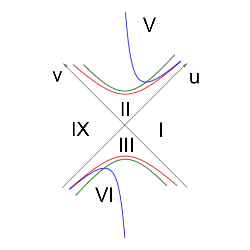
The physical interpretation of (2.15) is that of a scale invariant black hole. The corresponding Kruskal–Szekeres diagram is drawn in Figure 1 appearing later in subsection 2.4 and further comments will be presented there. This will be done in relation and comparison with that for the conformal case of [8] and as well as with that corresponding to the spacetime of the $\lambda$ -deformed model for the $\nicefrac{{SL(2,\mathbb{R})_{-k}}}{{SO(2)}}$ coset CFT.

2.2 Integrability

To prove the classical integrability of the action (2.13) we need to show that its equations of motion take the form of a Lax connection. For this purpose, we define

\begin{split}&{\cal L}_{\pm}^{1}=\frac{i}{2}\,\text{e}^{\tau}\,\zeta^{\pm 1}\sqrt{\lambda}\left(\partial_{\pm}\rho+\coth\rho\partial_{\pm}\tau\right)\,,\\ &{\cal L}_{\pm}^{2}=\pm\frac{1}{2}\text{e}^{\tau}\,\zeta^{\pm 1}\sqrt{\lambda}\left(\partial_{\pm}\rho+\coth\rho\partial_{\pm}\tau\right)\,,\\ &{\cal L}_{\pm}^{3}=\mp\frac{1}{2}\text{e}^{2\tau}\lambda\coth\rho\partial_{\pm}\rho\pm\frac{1}{2}\coth^{2}\rho(1-\lambda\text{e}^{2\tau})\partial_{\pm}\tau\,,\end{split}

(2.17)

where $\zeta$ is a complex parameter and we also introduce the matrix valued components

{\cal L}_{\pm}=\sum_{a=1}^{3}{\cal L}_{\pm}^{a}\sigma_{a}\,,

(2.18)

with $\sigma_{a}$ being the Pauli matrices. We have indeed checked that, the ${\cal L}_{\pm}$ ’s satisfy the flatness condition

\partial_{+}{\cal L}_{-}-\partial_{-}{\cal L}_{+}=[{\cal L}_{+},{\cal L}_{-}]\,,

(2.19)

provided that the equations of motion of the action (2.13) are satisfied. The existence of the Lax connection ensures integrability of (2.13), where $\zeta$ plays the rôle of a spectral parameter, in the weak sense. To prove integrability in the Hamiltonian sense we need to show that the conserved charges are in involution. In particular, we need to show that the spatial part of the Lax components (2.17), obeys the Maillet r/s-form [16, 17, 18]. This property is inherited from the $\lambda$ -deformed $\nicefrac{{SL(2,\mathbb{R})_{-k}}}{{SO(2)}}$ $\sigma$ -model, whose integrability in the weak and Hamiltonian sense were showed, respectively, in [19] and [20]. Its connection to (2.13) will be established later in the subsection 2.4.

2.3 Asymptotic limit and conformal invariance

Let now consider the large- $\rho$ limit of (2.13) and (2.2), yielding

\begin{split}S={k\over\pi}\int\text{d}^{2}\sigma\left(\partial_{+}\rho\partial_{-}\rho-\partial_{+}\tau\partial_{-}\tau+\lambda\,\text{e}^{2\tau}\partial_{+}(\rho+\tau)\partial_{-}(\rho+\tau)\right)\,,\end{split}

(2.20)

with the scalar $\Phi$ being equal to

\Phi=-\rho\,.

(2.21)

The corresponding target space geometry (in the normalization of (2.5)) is given by

\text{d}s^{2}=2k(\text{d}\rho^{2}-\text{d}\tau^{2})+\lambda V\ell_{\mu}\ell_{\nu}\text{d}X^{\mu}\text{d}X^{\nu}\,,

(2.22)

where

V=2k\text{e}^{2\tau}\,,\quad\ell_{\mu}\text{d}X^{\mu}=\text{d}\rho+\text{d}\tau\,,\quad X^{\mu}=(\rho,\tau)

(2.23)

and $\ell^{\mu}$ is a null and geodesic vector (1.1). Note that the line element (2.22) remains invariant under translations of $\rho$ and it is flat for $\lambda=0$ . Let us now work out the one-loop RG flows (2.6) for the target space metric (2.22) and the diffeomorphism

\xi^{\mu}\partial_{\mu}=g^{\mu\nu}\partial_{\nu}\Phi\partial_{\mu}+\frac{c}{2k}(\partial_{\rho}-\partial_{\tau})\quad\Longrightarrow\quad\xi_{\mu}\text{d}X^{\mu}=\text{d}\widehat{\Phi}\,,\quad\widehat{\Phi}=\Phi+c(\tau+\rho)\,,

(2.24)

where the scalar $\Phi$ is given by (2.21). The end result is given again by (2.16), where the parameter $\lambda$ can be absorbed in shifts of $\tau$ . Hence, we should pick $c=1$ corresponding to a conformal invariant $\sigma$ -model as the diffeomorphism can be written in terms of the dilaton field $\widehat{\Phi}=\tau$ .

In what follows, we will show that this model coincides with the $\nicefrac{{SL(2,\mathbb{R})_{k}}}{{SO(2)}}$ coset CFT by rewriting (2.20). To do so we perform the coordinate transformation

u=\text{e}^{-\rho-\tau}\,,\quad v=\frac{1}{\lambda}\text{e}^{\rho-\tau}+\text{e}^{\rho+\tau}

(2.25)

and we find the $\nicefrac{{SL(2,\mathbb{R})_{k}}}{{SO(2)}}$ coset CFT in global coordinates

S=\frac{k}{\pi}\int\text{d}^{2}\sigma\frac{\partial_{+}u\partial_{-}v}{1-uv}\,,\quad\Phi=-\frac{1}{2}\ln(1-uv)\,.

(2.26)

Finally, the target space of the aforementioned model has a cosmological interpretation [21], as we can see using the coordinate transformation

u=\cosh t\,\text{e}^{-r}\,,\quad v=\cosh t\,\text{e}^{r}\,,

(2.27)

leading to

S=\frac{k}{\pi}\int\text{d}^{2}\sigma\left(-\partial_{+}t\partial_{-}t+\coth^{2}t\partial_{+}r\partial_{-}r\right)\,.

(2.28)

2.4 Connection to the $\lambda$ -deformed integrable models

In this subsection, we will show that the action (2.13) can be derived from the $\lambda$ -deformed model based on the $\nicefrac{{SL(2,\mathbb{R})_{-k}}}{{SO(2)}}$ exact CFT [10]

	$\displaystyle S={k\over\pi}\int\text{d}^{2}\sigma\,\left\{\frac{1-\lambda}{1+\lambda}\big(\partial_{+}\rho\partial_{-}\rho-\coth^{2}\rho\,\partial_{+}\tau\partial_{-}\tau\big)\right.$		(2.29)
	$\displaystyle+\left.\frac{4\lambda}{1-\lambda^{2}}\big(\cosh\tau\,\partial_{+}\rho+\sinh\tau\,\coth\rho\,\partial_{+}\tau\big)\big(\cosh\tau\,\partial_{-}\rho+\sinh\tau\,\coth\rho\,\partial_{-}\tau\big)\right\}\ ,$

and the scalar

\Phi=-\ln\sinh\rho\,,

(2.30)

via a limiting procedure. Before that, let us first list some properties of (2.29). Inserting into (2.6) the target space of the action (2.29) and the diffeomorphism $\xi_{\mu}=\partial_{\mu}\Phi$ , with $\Phi$ being the dilaton (2.30), leads to the one-loop RG flow [22]

\frac{\text{d}\lambda}{\text{d}t}=\frac{\lambda}{k}\,,

(2.31)

where the level $k$ does not flow and the coset CFT $\nicefrac{{SL(2,\mathbb{R})_{-k}}}{{SO(2)}}$ is an IR fixed point at $\lambda=0$ . The action (2.29) describes irrelevant perturbations around the conformal point $\lambda=0$ , whose target space describes the black hole of [8] beyond the singularity. This is consistent with the Weyl anomaly coefficient

W=2-3(R+4\nabla^{2}\Phi-4(\nabla\Phi)^{2})=2+\frac{6}{k}\frac{1+\lambda^{2}}{1-\lambda^{2}}\,,

(2.32)

matching Zamolodchikov’s $C$ -function [23, 24] and it satisfies the $c$ -theorem [25]. In addition, the model (2.29) is classically integrable as its equations of motion take the form of a Lax connection [19] and it is also integrable in the Hamiltonian sense as its conserved charges are in involution [20]. Finally, (2.29) may be rewritten in a conformally flat form in global coordinates [11]

S=k\frac{1-\lambda^{2}}{\pi}\int\text{d}^{2}\sigma\frac{\partial_{+}u\partial_{-}v}{(u-\lambda v)(v-\lambda u)-(1-\lambda^{2})^{2}}\,,

(2.33)

after the transformation

u=\cosh\rho\left(\text{e}^{-\tau}+\lambda\text{e}^{\tau}\right)\,,\quad v=\cosh\rho\left(\text{e}^{\tau}+\lambda\text{e}^{-\tau}\right)\,

(2.34)

and a subsequent extension of the range of the new variables $u$ and $v$ .

As advertized above the Kerr–Schild deformation of the coset CFT $\nicefrac{{SL(2,\mathbb{R})_{-k}}}{{SO(2)}}$ (2.13) can be obtained from the $\lambda$ -deformed corresponding coset CFT (2.29) using a limiting procedure. The appropriate limit, asymptotic and simultaneously taking the deformation parameter to zero in a correlated way, is

\tau\to\tau-\frac{1}{2}\ln\varepsilon\,,\quad\lambda\to\varepsilon\lambda\quad\text{with}\quad\varepsilon\to 0\,.

(2.35)

Equivalently, (2.15) could be reached from (2.33) in the limit

u\to\sqrt{\varepsilon\lambda}u\,,\quad v\to\frac{v}{\sqrt{\varepsilon\lambda}}\,,\quad\lambda\to\varepsilon\lambda\quad\text{with}\quad\varepsilon\to 0\,.

(2.36)

The Lax connections of the actions (2.13) and (2.29) coincide in the limit (2.35).⁶⁶ 6 More precisely the Lax connection of the $\lambda$ -deformed action (2.29), as it was constructed in [19], turns out to depend on all three group parameters of the original $SL(2,\mathbb{R})$ element. One of them can be absorbed in a gauge transformation of the Lax connection, that is ${\cal L}_{\pm}\to h^{-1}{\cal L}_{\pm}h-h^{-1}\partial_{\pm}h$ with $h\in SO(2)$ . Alternatively, one may fix one of the parameters thanks to the $SO(2)$ gauge invariance. This property also proves the integrability of the action (2.13) in the Hamiltonian sense.

Finally, we would like to consider the large- $\rho$ limit in (2.29) and (2.30) and to make contact with the results of [26]. Doing so we find

	$\displaystyle S={k\over\pi}\int\text{d}^{2}\sigma\,\left\{\frac{1-\lambda}{1+\lambda}\big(\partial_{+}\rho\partial_{-}\rho-\,\partial_{+}\tau\partial_{-}\tau\big)\right.$		(2.37)
	$\displaystyle+\left.\frac{4\lambda}{1-\lambda^{2}}\big(\cosh\tau\,\partial_{+}\rho+\sinh\tau\,\partial_{+}\tau\big)\big(\cosh\tau\,\partial_{-}\rho+\sinh\tau\,\partial_{-}\tau\big)\right\}$

and the scalar $\Phi=-\rho$ . The latter background interpolates between a free scalar times a linear dilaton background in the IR and the $\text{AdS}_{2}$ space towards the UV [26].⁷⁷ 7 Upon taking the large- $\tau$ limit (2.35) yields again (2.20). Hence, the large- $\rho$ and - $\tau$ limits commute.

For completeness, we also present the conformally flat form of (2.37)

S=k\frac{1-\lambda^{2}}{\pi}\int\text{d}^{2}\sigma\frac{\partial_{+}u\partial_{-}v}{(u-\lambda v)(v-\lambda u)}.

(2.38)

where

u=\frac{\text{e}^{\rho}}{2}\left(\text{e}^{-\tau}+\lambda\text{e}^{\tau}\right)\,,\quad v=\frac{\text{e}^{\rho}}{2}\left(\text{e}^{\tau}+\lambda\text{e}^{-\tau}\right)\,,

(2.39)

which can be viewed as the large- $\rho$ limit of (2.33) and (2.34), respectively.⁸⁸ 8 The limit of $\lambda=1-\nicefrac{{\kappa^{2}}}{{k}}$ as $k\gg 1$ towards the UV, can be easily taken in (2.38) leading to the $\text{AdS}_{2}$ metric expressed in Poincaré coordinates $S=\frac{\kappa^{2}}{2\pi}\int\text{d}^{2}\sigma\,\frac{1}{z^{2}}\left(\partial_{+}z\partial_{-}z-\partial_{+}t\partial_{-}t\right)\,.$ A similar conclusion, with a slightly different reasoning, has been reached in [11].

We have drawn the Kruskal–Szekeres diagrams in Figure 1 for the actions (2.15) and (2.33) (for generic $\lambda$ and for $\lambda=0$ ) depicting the positions of the horizons at $u=0$ and at $v=0$ , as well as of the singularity curves corresponding to the vanishing of the functions in the denominators in the corresponding $\sigma$ -model actions. Defining $v=T-X$ and $u=T+X$ , in regions I-IV the time $T$ flows upwards whereas in the regions V and VI sideways. The discussion is completely analogous to that in [8].

Refer to caption — Figure 1: The Kruskal–Szekeres diagrams of the scale invariant (2.15) and the $\lambda$ -deformed model (2.33) (for $\lambda\neq 0$ ), showing the location of the singularity, in blue and green colors, respectively. In red is the singularity at $uv=1$ in the CFT case (for $\lambda=0$ ) of [8]. The blue curve is not left-right symmetric since the limit (2.36) breaks that symmetry.

2.5 Embedding to supergravity

The embedding to supergravity can be found by taking the asymptotic limit (2.35) in the solution corresponding to the embedding of the $\lambda$ -deformed $\nicefrac{{SL(2,\mathbb{R})_{-k}}}{{SO(2)}}$ non-compact CFT times the $\lambda$ -deformed $\nicefrac{{SU(2)_{k}}}{{U(1)}}$ compact CFT backgrounds. This was done in Section 5.3 of [11] and we emphasize that it is necessary to consider both $\lambda$ -deformed spaces in order for the embedding to be achieved. Upon applying the asymptotic limit (2.35) its NS sector is given by

\small\begin{split}&\text{d}s^{2}=2k\left\{\text{d}\rho^{2}-\coth^{2}\rho\text{d}\tau^{2}+\text{d}\omega^{2}+\cot^{2}\omega\text{d}\phi^{2}+\lambda\text{e}^{2\tau}\,(\text{d}\rho+\coth\rho\text{d}\tau)^{2}\right\}+\sum_{i=1}^{6}\text{d}x_{i}^{2}\,,\\ &\text{e}^{-2\Phi}=\sin^{2}\omega\sinh^{2}\rho\,.\end{split}

(2.40)

These fields have to be supported by RR-flux forms in order to satisfy the type-II supergravity equations.

The embedding to type-IIA supergravity requires the two- and four-forms

\begin{split}&F_{2}=\sqrt{2k\lambda}\,\text{e}^{\tau}(\cosh\rho\text{d}\tau+\sinh\rho\text{d}\rho)\wedge(\cos\omega\sin\phi\,\text{d}\phi+\cos\phi\sin\omega\,\text{d}\omega)\,,\\ &F_{4}=\sqrt{2k\lambda}\,\text{e}^{\tau}(\cosh\rho\text{d}\tau+\sinh\rho\text{d}\rho)\wedge(\cos\omega\cos\phi\,\text{d}\phi-\sin\phi\sin\omega\,\text{d}\omega)\wedge J_{2}\,,\\ &J_{2}=\text{d}x_{12}+\text{d}x_{34}+\text{d}x_{56}\,,\end{split}

(2.41)

where we have used the standard notation $\text{d}x_{12}=\text{d}x_{1}\wedge\text{d}x_{2}$ , etc.

Similarly, the embedding to type-IIB supergravity requires the five-form

\begin{split}&F_{5}=(1+\ast)f_{5}\,,\\ &f_{5}=\sqrt{2k\lambda}\,\text{e}^{\tau}(\cosh\rho\text{d}\tau+\sinh\rho\text{d}\rho)\wedge(\cos\omega\sin\phi\text{d}\phi+\cos\phi\sin\omega\,\text{d}\omega)\wedge J_{3}\,,\\ &J_{3}=\text{d}x_{135}-\text{d}x_{146}-\text{d}x_{245}-\text{d}x_{236}\,.\end{split}

(2.42)

These supergravity backgrounds turn out to be non-supersymmetric as one can easily see by analyzing the dilatino variation.

3 Kerr–Schild deformation of a 3-dim target space CFT

We would like to extend the results of the previous section to higher dimensional examples. However, a brut force analysis turns out to be rather tedious and for this reason we will consider analogue asymptotic limits of $\lambda$ -deformed orthogonal coset CFTs, along the lines of Subsection 2.4.

Let us first consider the three-dimensional gauged WZW models for orthogonal groups. The target space consists of a metric and a dilaton given in terms of [12]

\text{d}s^{2}=2k\left(\frac{\text{d}b^{2}}{b^{2}-1}+\frac{b-1}{b+1}\frac{\text{d}u^{2}}{u(v-u-2)}-\frac{b+1}{b-1}\frac{\text{d}v^{2}}{v(v-u-2)}\right)

(3.1)

and

\text{e}^{-2\Phi}=(b^{2}-1)(v-u-2)\,,

(3.2)

which are valid for large $k$ . The various cosets appear for different ranges of the global coordinates $(u,v,b)$ and are summarized in Eq. (30) of [27], see also below for the reader’s convenience

•

$\text{CAdS}_{3,k}=\nicefrac{{SO(2,2)_{-k}}}{{SO(2,1)_{-k}}}$

$\left\{|b|>1,uv>0\right\}\quad\text{or}\quad\left\{|b|<1,uv<0\ \text{excluding}\ 0<v<u+2<2\right\};$ (3.3)
•

$\text{CdS}_{3,k}=\nicefrac{{SO(3,1)_{k}}}{{SO(2,1)_{k}}}$

$\left\{|b|<1,uv>0\right\}\quad\text{or}\quad\left\{|b|>1,uv<0\ \text{excluding}\ 0<v<u+2<2\right\};$ (3.4)
•

$\text{CH}_{3,k}=\nicefrac{{SO(3,1)_{-k}}}{{SO(3)_{-k}}}$

$\left\{|b|>1,0<v<u+2<2\right\};$ (3.5)
•

$\text{CS}_{3,k}=\nicefrac{{SO(4)_{k}}}{{SO(3)_{k}}}$

$\left\{|b|<1,0<v<u+2<2\right\}.$ (3.6)

The first two have Minkowskian signature and the remaining ones Euclidean. Also, note that, none of these spaces enjoys any Killing vector.

3.1 The integrable $\lambda$ -deformation of the $\nicefrac{{SO(2,2)_{-k}}}{{SO(2,1)_{-k}}}$ coset CFT

The $\lambda$ -deformed version of (3.1) was constructed in [28]. In our global coordinates the metric is given by

	$\displaystyle\text{d}s_{\lambda}^{2}=2k\bigg(\frac{1+\lambda^{2}+2\lambda(v-u-1)}{1-\lambda^{2}}\frac{\text{d}b^{2}}{b^{2}-1}+\frac{1+b}{1-b}\frac{1+\lambda^{2}+2\lambda(1-v)}{1-\lambda^{2}}\frac{\text{d}v^{2}}{v(v-u-2)}$
	$\displaystyle\qquad-\frac{1-b}{1+b}\frac{1+\lambda^{2}+2\lambda(1+u)}{1-\lambda^{2}}\frac{\text{d}u^{2}}{u(v-u-2)}-\frac{4\lambda}{1-\lambda^{2}}\frac{\text{d}u\,\text{d}v}{v-u-2}$		(3.7)
	$\displaystyle\qquad-\frac{4\lambda}{1-\lambda^{2}}\frac{\text{d}b\,\text{d}u}{1+b}-\frac{4\lambda}{1-\lambda^{2}}\frac{\text{d}b\,\text{d}v}{1-b}\bigg)\,,$

where the dilaton is still given by (3.2). This model is classically integrable since the equations of motion can be written in terms of a Lax connection [19] and its conserved charges are in involution [20]. The $\sigma$ -model (3.1) is renormalizable at one-loop order in the $\nicefrac{{1}}{{k}}$ expansion. Indeed, inserting (3.1), (3.2) into (2.6), leads to the one-loop RG flow [29, 30]

\beta^{\lambda}=\frac{\text{d}\lambda}{\text{d}t}=\frac{\lambda}{2k}\,,

(3.8)

where the CFT point $\lambda=0$ is an IR fixed point. In addition, the Weyl anomaly coefficient in the case at hand reads [23, 24]

W=3-3(R+4\nabla^{2}\Phi-4(\nabla\Phi)^{2})=3+\frac{9}{2k}\frac{1+\lambda^{2}}{1-\lambda^{2}}\,,

(3.9)

which is identified with the Zamolodchikov’s c-function [25].

3.2 The Kerr–Schild asymptotic limit

Let us now consider the metric (3.1) in the parametric region of (3.3) or (3.4) and take a variant of the limit considered in [31], followed by taking the parameter $\lambda$ to zero. Specifically,

(u,v)\to\frac{1}{\varepsilon}(u,v)\,,\quad\lambda\to\varepsilon\lambda\quad\text{with}\quad\varepsilon\to 0\,.

(3.10)

Applying this limit to (3.1) we find that

\small\begin{split}&\text{d}s^{2}=2k\left(\frac{\text{d}b^{2}}{b^{2}-1}+\frac{b-1}{b+1}\frac{\text{d}u^{2}}{u(v-u)}-\frac{b+1}{b-1}\frac{\text{d}v^{2}}{v(v-u)}\right)+\lambda\,V\ell_{\mu}\ell_{\nu}\text{d}X^{\mu}\text{d}X^{\nu}\,,\\ &\ell=\text{d}\left[(b+1)v-(b-1)u\right]\,,\hskip 9.24994ptV=\frac{4\,k}{(b^{2}-1)(v-u)}\,,\hskip 9.24994ptX^{\mu}=(b,u,v)\,.\end{split}

(3.11)

The vector $\ell^{\mu}$ is null and geodesic obeying (1.1). The dilaton is obtained from (3.2) and equals to

\text{e}^{-2\Phi}=(b^{2}-1)(v-u)\,,

(3.12)

where an $\varepsilon$ -depended constant has been disregarded by redefining the additive constant that we may always add to the dilaton. Note that the $\lambda$ -independent term in (3.11) develops an invariance involving the same scaling of the variables $u$ and $v$ , which is not present in the original metric (3.1). This invariance is broken by the dilaton field (3.12),⁹⁹ 9 This property was used in [32], where the authors performed an Abelian T-duality in the background (3.11) (for $\lambda=0$ ), but for the range of variables corresponding to the $CH_{3,k}$ coset CFT in (3.4), with respect to the aforementioned scaling symmetry. Due to the non-invariance of the dilaton the result is not expected to be and in fact it is not, a conformal background. Nevertheless, it turns out to be scale invariant. but also by the $\lambda$ -dependent term in (3.11).

We note that this is a different limit than the one taken in [26]. In that work we considered (3.1) in the parametric region of (3.5) and took the asymptotic limit $b\to\infty$ leaving the parameter $\lambda$ intact. The derived $\sigma$ -model interpolates under RG flow between the $\nicefrac{{SO(3)_{k}}}{{SO(2)}}$ coset CFT times a linear dilaton in the IR [27] towards an $H_{3}$ hyperbolic space in the UV as $\lambda\to 1$ [26].

3.3 Scale invariance

Let us now study the one-loop RG flows (2.6) for the target space (3.11), where we consider the diffeomorphism

\xi^{\mu}\partial_{\mu}=g^{\mu\nu}\partial_{\nu}\Phi\,\partial_{\mu}+\eta\,,\quad\eta=-\frac{c}{2k}\left(u\,\partial_{u}+v\,\partial_{v}\right),

(3.13)

with $c$ being an arbitrary parameter. Similarly to (2.7) the second term involves a diffeomorphism corresponding to the scale invariance of the $\lambda$ -independent term in (3.11). This $\eta$ diffeomorphism cannot be written in terms of a new scalar and its Lie derivative is given by

\nabla_{\mu}\eta_{\nu}+\nabla_{\nu}\eta_{\mu}=-\frac{2\lambda c}{(b^{2}-1)(v-u)}\ell_{\mu}\ell_{\nu}\,,

(3.14)

which is similar to (2.9). Employing the one-loop RG flows (2.6) and the diffeomorphism (3.13), one finds

\frac{\text{d}\lambda}{\text{d}t}=(1-c)\frac{\lambda}{2k}\,,

(3.15)

whereas the level $k$ does not flow at this order. Following a similar reasoning as in the two-dimensional case we choose $c=1$ . Hence, (3.11) corresponds to a scale invariant $\sigma$ -model for $\lambda$ different than zero and to a Weyl invariant one for $\lambda$ equal to zero.

3.4 Asymptotic limit and conformal invariance

Let us now consider the large- $b$ limit of (3.11) and (3.12), yielding

\begin{split}\text{d}s^{2}&=2k\left(\frac{\text{d}b^{2}}{b^{2}}+\frac{\text{d}u^{2}}{u(v-u)}-\frac{\text{d}v^{2}}{v(v-u)}\right)+\frac{4k\lambda}{b^{2}(v-u)}\ell_{\mu}\ell_{\nu}\text{d}X^{\mu}\text{d}X^{\nu}\,,\end{split}

(3.16)

where $\ell_{\mu}\text{d}X^{\mu}=\text{d}[b(v-u)]$ , with $X^{\mu}=(b,u,v)$ and

\text{e}^{-2\Phi}=b^{2}(v-u)\,.

(3.17)

The latter line element remains invariant under rescalings of $b$ as well and it is flat for $\lambda=0$ . Let us now work out the one-loop RG flows (2.6) for the above metric with the diffeomorphism

\xi^{\mu}\partial_{\mu}=g^{\mu\nu}\partial_{\nu}\Phi\,\partial_{\mu}-\frac{c}{2k}\left(-b\partial_{b}+u\,\partial_{u}+v\,\partial_{v}\right)\quad\Longrightarrow\quad\xi_{\mu}\text{d}X^{\mu}=\text{d}\widehat{\Phi}\,,

(3.18)

where $\widehat{\Phi}=\Phi+c\ln[b(v-u)]$ . The above diffeomorphism yields the RG flow (3.15) and the parameter $\lambda$ can be also absorbed in (unphysical) rescalings of $(u,v)$ . Hence, we should pick $c=1$ corresponding to a conformal invariant $\sigma$ -model since the diffeomorphism is expressed in terms of a new dilaton field $\widehat{\Phi}=\nicefrac{{1}}{{2}}\ln(v-u)$ .

We conclude by identifying the corresponding CFT. To do so, we perform the following coordinate transformation in (3.16)

v=\text{e}^{2\tau}\cosh^{2}y\,,\quad u=\text{e}^{2\tau}\sinh^{2}y\,,\quad b=\text{e}^{2\rho}\,.

(3.19)

The corresponding $\sigma$ -model (in the normalization of (2.5)) reads

S={4k\over\pi}\int\text{d}^{2}\sigma\left(\partial_{+}\rho\partial_{-}\rho-\partial_{+}\tau\partial_{-}\tau+\partial_{+}y\partial_{-}y+4\lambda\,\text{e}^{2\tau}\partial_{+}(\rho+\tau)\partial_{-}(\rho+\tau)\right)

(3.20)

and the dilaton equals to $\widehat{\Phi}=\tau$ . Following the discussion in Subsection 2.3 we find that the model (3.20) describes the $\nicefrac{{SL(2,\mathbb{R})_{4k}}}{{SO(2)}}\times\mathbb{R}$ CFT.

4 Conclusions

In the present work we studied Kerr–Schild deformation of coset CFTs of a non-compact target spacetime. Firstly, we considered deformations of the two-dimensional coset CFT $\nicefrac{{SL(2,\mathbb{R})_{-k}}}{{SO(2)}}$ [8]. The derived $\sigma$ -model is classically integrable and scale rather than Weyl invariant. The target spacetime of this model has the interpretation of a scale invariant black hole which we embed in type-IIA and -IIB supergravity. We show that this type of deformation can be obtained from the corresponding $\lambda$ -deformed model by performing a particular limiting procedure. Finally, in an asymptotic limit the model becomes Weyl invariant, in particular the coset CFT $\nicefrac{{SL(2,\mathbb{R})_{k}}}{{SO(2)}}$ .

We extended the above results in a three-dimensional model where we considered a similar limiting procedure of the $\lambda$ -deformed $\nicefrac{{SO(2,2)_{-k}}}{{SO(2,1)_{-k}}}$ coset CFT. The derived model can be viewed again as a Kerr–Schild deformation of an asymptotic limit of the underlying $\nicefrac{{SO(2,2)_{-k}}}{{SO(2,1)_{-k}}}$ coset CFT. As in the two-dimensional case, the model is classically integrable and in addition scale invariant. Weyl invariance is restored in an asymptotic limit, yielding the $\nicefrac{{SL(2,\mathbb{R})_{4k}}}{{SO(2)}}\times\mathbb{R}$ CFT.

The results of the present work could be extended for higher dimensional symmetric coset CFTs by taking appropriate limiting procedures of the corresponding $\lambda$ -deformed models. In fact we have explicitly checked the four- and five-dimensional cases, namely the $\lambda$ -deformed $\nicefrac{{SO(3,2)_{-k}}}{{SO(3,1)_{-k}}}$ and $\nicefrac{{SO(4,2)_{-k}}}{{SO(4,1)_{-k}}}$ $\sigma$ -models. We will not present any details of this technically involved analysis since the results are identical to the two- and three-dimensional cases.

A natural question is whether scale invariance persists beyond one-loop. The simplest such exact background corresponds to the coset CFT $\nicefrac{{SL(2,\mathbb{R})_{-k}}}{{SO(2)}}$ and it was found in [33, 34]. We have studied its two-loop renormalizability [35, 36, 37, 38, 39] under Kerr–Schild deformation and indeed we have found that scale invariance persists. We refrain from presenting the details of the intermediate steps as they are complicated and its conceptual core remains intact.

Another potential extension would be to consider Kerr–Schild deformation of Yang–Baxter symmetric cosets which were constructed in [40, 41]. These types of $\sigma$ -models are related to the $\lambda$ -deformed ones by a Poisson–Lie T-duality and an analytic continuation of the coordinates and parameters of the underlying $\sigma$ -model [42, 43, 44, 45, 46].

Acknowledgements

We would like to thank Nat Levine and Arcady Tseytlin for a useful correspondence and Andreas Stergiou for related discussions.
We also thank the organizers and the participants of the conference “Integrability, Dualities and Deformations" (Santiago de Compostela, Spain, 30 August – 3 September 2021) for the stimulating atmosphere, where results of this work were presented by K. Siampos.
The research work of G. Itsios is supported by the Einstein Stiftung Berlin via the Einstein International Postdoctoral Fellowship program “Generalised dualities and their holographic applications to condensed matter physics” (project number IPF-2020-604). G. Itsios is also supported by the Deutsche Forschungsgemeinschaft (DFG, German Research Foundation) via the Emmy Noether program “Exploring the landscape of string theory flux vacua using exceptional field theory” (project number 426510644).
The research work of K. Sfetsos was supported by the Hellenic Foundation for Research and Innovation (H.F.R.I.) under the “First Call for H.F.R.I. Research Projects to support Faculty members and Researchers and the procurement of high-cost research equipment grant” (MIS 1857, Project Number: 16519).
The research work of K. Siampos has received funding from the Hellenic Foundation for Research and Innovation (H.F.R.I.) and the General Secretariat for Research and Technology (G.S.R.T.), under grant agreement No 15425.

Appendix A Essentials of Kerr–Schild perturbations

In this section we will consider metric perturbations of the Kerr–Schild form [1, 2, 3, 4, 5, 6]

g_{\mu\nu}=g^{(0)}_{\mu\nu}+\lambda\,h_{\mu\nu}\,,\quad h_{\mu\nu}=V\ell_{\mu}\ell_{\nu}\,,\quad\mu=1,2,\dots,D\,,

(A.1)

where $\lambda$ is a booking keeping (expansion) parameter and $V$ is the Kerr–Schild potential. In addition, the vector $\ell^{\mu}$ is null and geodesic

g^{(0)}_{\mu\nu}\ell^{\mu}\ell^{\nu}=0=g_{\mu\nu}\ell^{\mu}\ell^{\nu}\,,\quad\ell^{\mu}\nabla^{(0)}_{\mu}\ell_{\nu}=0\,.

(A.2)

From the above it can be easily seen that the inverse of the metric (A.1) is given by

g^{\mu\nu}=g_{(0)}^{\mu\nu}-\lambda h^{\mu\nu}\,,\quad h^{\mu\nu}=V\ell^{\mu}\ell^{\nu}\,.

(A.3)

Using the latter and (A.2), we find the Christoffel symbols

\Gamma_{\kappa\lambda}{}^{\mu}=\Gamma^{(0)}_{\kappa\lambda}{}^{\mu}+S_{\kappa\lambda}{}^{\mu}\,,

(A.4)

where

\begin{split}S_{\kappa\lambda}{}^{\mu}&=\lambda S^{(1)}_{\kappa\lambda}{}^{\mu}+\lambda^{2}S^{(2)}_{\kappa\lambda}{}^{\mu}\,,\\ S^{(1)}_{\kappa\lambda}{}^{\mu}&=\frac{1}{2}g^{\mu\rho}\left(\nabla^{(0)}_{\kappa}h_{\lambda\rho}+\nabla^{(0)}_{\lambda}h_{\kappa\rho}-\nabla^{(0)}_{\rho}h_{\kappa\lambda}\right)\,,\\ S^{(2)}_{\kappa\lambda}{}^{\mu}&=\frac{1}{2}h^{\mu\rho}\nabla^{(0)}_{\rho}h_{\kappa\lambda}=\frac{1}{2}h^{\mu\rho}h_{\kappa\lambda}\partial_{\rho}\ln V\,.\end{split}

(A.5)

Using the above one may easily demonstrate that the geodesic property of the vector holds for the metric $g_{\mu\nu}$ as well, i.e.

\ell^{\mu}\nabla_{\mu}\ell_{\nu}=0\,.

(A.6)

We also note the property

S^{(i)}_{\kappa\lambda}{}^{\lambda}=0\,,\quad i=1,2.

(A.7)

Next we evaluate the Riemann tensor, which takes the form

R^{\mu}{}_{\rho\kappa\lambda}=R^{(0)\mu}{}_{\rho\kappa\lambda}+\nabla^{(0)}_{\kappa}S_{\lambda\rho}{}^{\mu}-\nabla^{(0)}_{\lambda}S_{\kappa\rho}{}^{\mu}+S_{\kappa\sigma}{}^{\mu}S_{\lambda\rho}{}^{\sigma}-S_{\lambda\sigma}{}^{\mu}S_{\kappa\rho}{}^{\sigma}\,,

(A.8)

implying that the corresponding Ricci tensor could be at most fourth order in $\lambda$ . Using (A.2), we find after some algebra that the Ricci tensor truncates at second order in $\lambda$ and it is given by

R_{\mu\nu}=R^{(0)}_{\mu\nu}+\lambda R^{(1)}_{\mu\nu}+\lambda^{2}R^{(2)}_{\mu\nu}\,,

(A.9)

where

\begin{split}R_{\mu\nu}^{(1)}&=\frac{1}{2}\nabla^{(0)\rho}\left(\nabla^{(0)}_{\mu}h_{\nu\rho}+\nabla^{(0)}_{\nu}h_{\mu\rho}-\nabla^{(0)}_{\rho}h_{\mu\nu}\right)\,,\\ R_{\mu\nu}^{(2)}&=\frac{1}{2}\left(\nabla^{(0)}_{k}(\ell^{k}\ell^{\lambda}\partial_{\lambda}V)+V\,\big(\nabla^{(0)}_{\kappa}\ell_{\lambda}\big)(\nabla^{(0)\kappa}\ell^{\lambda}-\nabla^{(0)\lambda}\ell^{\kappa})\right)h_{\mu\nu}\,.\end{split}

(A.10)

The above can be rewritten as¹⁰¹⁰ 10 Where we have used the identity $V\left(\nabla^{(0)}_{\kappa}(\ell^{\kappa}\ell^{\lambda}\partial_{\lambda}V)+V(\nabla^{(0)}_{\kappa}\ell_{\sigma}-\nabla^{(0)}_{\kappa}\ell_{\sigma})\nabla^{(0)\sigma}\ell^{\kappa}\right)=h_{\mu}{}^{\sigma}\nabla^{(0)\rho}\left(\nabla^{(0)}_{\nu}h_{\sigma\rho}+\nabla^{(0)}_{\sigma}h_{\rho\nu}-\nabla^{(0)}_{\rho}h_{\sigma\nu}\right)\,.$

\begin{split}R_{\mu\nu}&=R^{(0)}_{\mu\nu}+\frac{\lambda}{2}\nabla^{(0)\rho}\left(\nabla^{(0)}_{\mu}h_{\nu\rho}+\nabla^{(0)}_{\nu}h_{\mu\rho}-\nabla^{(0)}_{\rho}h_{\mu\nu}\right)\\ &+\frac{\lambda^{2}}{2}h_{\mu}{}^{\sigma}\nabla^{(0)\rho}\left(\nabla^{(0)}_{\nu}h_{\sigma\rho}+\nabla^{(0)}_{\sigma}h_{\rho\nu}-\nabla^{(0)}_{\rho}h_{\sigma\nu}\right)\,.\end{split}

(A.11)

or in the suggestive form

R^{\mu}{}_{\nu}=R^{(0)\mu}{}_{\nu}-\lambda h^{\mu}{}_{\rho}R^{(0)\rho}{}_{\nu}+\frac{\lambda}{2}\nabla^{(0)}_{\rho}\left(\nabla^{(0)}_{\nu}h^{\mu\rho}+\nabla^{(0)\mu}h_{\nu}{}^{\rho}-\nabla^{(0)\rho}h^{\mu}{}_{\nu}\right)\,.

(A.12)

This unveils that in this case the linearized approximation is also an exact,¹¹¹¹ 11 This property is realized in the mixed components form (A.12); with one index up and one down. where the metric $g_{\mu\nu}$ is given by (A.1) and $\ell^{\mu}$ satisfies (A.2). This has been observed in [5]. Finally, we can also compute the Ricci tensor

R=R^{(0)}-\lambda h^{\mu\nu}R^{(0)}_{\mu\nu}+\lambda\nabla^{(0)}_{\mu}\left(\nabla^{(0)}_{\nu}\left(V\ell^{\nu}\right)\ell^{\mu}\right)\,.

(A.13)

As a non-trivial example of the Kerr–Schild formulation [1] we present the renowned Kerr solution of mass $M$ and rotation parameter $a$ , in the presence of a cosmological constant $\Lambda$ . The first step is to rewrite the (A)dS metric, which will be the seed solution, in a rotating form using spheroidal coordinates[47] and in the conventions of [48]

\begin{split}g^{(0)}_{\mu\nu}\text{d}x^{\mu}\text{d}x^{\nu}&=-\frac{\Delta}{\Omega}\left(1+\frac{\Lambda r^{2}}{3}\right)\text{d}t^{2}+\frac{r^{2}+a^{2}\cos^{2}\theta}{r^{2}+a^{2}}\frac{\text{d}r^{2}}{1+\frac{\Lambda r^{2}}{3}}\\ &+\frac{r^{2}+a^{2}\cos^{2}\theta}{\Delta}\text{d}\theta^{2}+\frac{(r^{2}+a^{2})\sin^{2}\theta}{\Omega}\text{d}\phi^{2}\,,\end{split}

(A.14)

where

\Delta=1-\frac{\Lambda}{3}a^{2}\cos^{2}\theta\,,\quad\Omega=1-\frac{\Lambda}{3}a^{2}\,.

(A.15)

It turns out that the Kerr–Schild potential $V$ and the null and geodesic vector $\ell^{\mu}$ read

V=\frac{2GMr}{r^{2}+a^{2}\cos^{2}\theta}\,,\quad\ell=-\frac{\Delta}{\Omega}\text{d}t+\frac{r^{2}+a^{2}\cos^{2}\theta}{r^{2}+a^{2}}\frac{\text{d}r}{1+\frac{\Lambda r^{2}}{3}}-\frac{a\sin^{2}\theta}{\Omega}\text{d}\phi\,,

(A.16)

such that $R_{\mu\nu}=\Lambda g_{\mu\nu}$ .

Further investigations and examples concerning Kerr–Schild perturbations can found in [49, 50, 51].

References

[1] R. P. Kerr, A. Schild, A new class of vacuum solutions of the Einstein field equations, Atti del Convegno sulla Relativita Generale: Problemi dell’Energia e Onde Gravitazionali, G. Barbèra Editore, Firenze (1965), 1-12 and
General Relativity and Gravitation. 41 (2009), 2485-2499.
Some algebraically degenerate solutions of Einstein’s gravitational field equations,
Proc. Symp. Appl. Math. 17 (1965), 199-209.
[2] M. Gürses and F. Gürsey, Lorentz covariant treatment of the Kerr-Schild geometry,
J. Math. Phys. 16 (1975), 2385-2390.
[3] B. C. Xanthopoulos, Exact vacuum solutions of Einstein’s equation from linearized solutions, J. Math. Phys. 19 (1978), 1607-1609.
[4] A. H. Taub, Generalised Kerr-Schild space-times,
Ann. Phys. 134 Issue 2 (1981), 326-372.
[5] T. Dereli and M. Gürses, The Generalized Kerr-schild Transform in Eleven-dimensional Supergravity, Phys. Lett. B171 (1986), 209-211.
[6] B. C. Xanthopoulos, Linear superposition of solutions of the Einstein-Maxwell equations, Class. Quant. Grav. 3 (1986), 157-167.
[7] H. Stephani, D. Kramer, M. MacCallum, C. Hoenselaers and E. Herlt,
Exact solutions to Einstein’s field equations, (2nd ed., Cambridge Monographs on Mathematical Physics). Cambridge: Cambridge University Press, doi:10.1017/CBO9780511535185.
[8] E. Witten, On string theory and black holes, Phys. Rev. D44 (1991), 314-324.
[9] C. M. Hull and P. K. Townsend, Finiteness and Conformal Invariance in Nonlinear $\sigma$ -Models, Nucl. Phys. B274 (1986), 349-362.
[10] K. Sfetsos, Integrable interpolations: From exact CFTs to non-Abelian T-duals, Nucl. Phys. B880 (2014), 225-246, [1312.4560].
[11] K. Sfetsos and D. C. Thompson, Spacetimes for $\lambda$ -deformations,
JHEP 12 (2014), 164 (26pp), [1410.1886].
[12] I. Bars and K. Sfetsos, Global analysis of new gravitational singularities in string and particle theories, Phys. Rev. D46 (1992), 4495-4509, [hep-th/9205037].
[13] G. Ecker and J. Honerkamp, Application of invariant renormalization to the nonlinear chiral invariant pion Lagrangian in the one-loop approximation, Nucl. Phys. B35 (1971), 481-492. J. Honerkamp, Chiral multiloops, Nucl. Phys. B36 (1972), 130-140.
[14] D. Friedan, Nonlinear models in two epsilon dimensions, Phys. Rev. Lett. 45 (1980), 1057-1060 and Nonlinear models in $2+\varepsilon$ dimensions, Annals Phys. 163 (1985), 318-419.
[15] J. Polchinski, Scale and conformal invariance in quantum field theory,
Nucl.Phys. B303 (1988), 226-236.
[16] E. K. Sklyanin, Quantum version of the method of inverse scattering problem,
J. Sov. Math. 19 (1982), 1546-1596, Zap. Nauchn. Semin. 95 (1980), 55-128.
[17] J. M. Maillet, New Integrable Canonical Structures in Two-dimensional Models,
Nucl. Phys. B269 (1986), 54-76.
[18] J. M. Maillet, Hamiltonian Structures for Integrable Classical Theories From Graded Kac-moody Algebras, Phys. Lett. B167 (1986), 401-405.
[19] T. J. Hollowood, J. L. Miramontes and D. M. Schmidtt, Integrable deformations of strings on symmetric spaces, JHEP 1411 (2014), 009 (35pp), [1407.2840].
[20] T. J. Hollowood, J. L. Miramontes and D. M. Schmidtt, S-Matrices and Quantum Group Symmetry of k-Deformed Sigma Models,
J. Phys. A 49 no.46 (2016), 465201 (25pp), [1506.06601].
[21] C. Kounnas and D. Lüst, Cosmological string backgrounds from gauged WZW models, Phys. Lett. B289 (1992), 56-60, [hep-th/9205046].
[22] G. Itsios, K. Sfetsos and K. Siampos, The all-loop non-Abelian Thirring model and its RG flow, Phys. Lett. B733 (2014), 265-269, [1404.3748].
[23] G. Georgiou, P. Panopoulos, E. Sagkrioti, K. Sfetsos and K. Siampos, The exact $C$ -function in integrable $\lambda$ -deformed theories,
Phys. Lett. B782 (2018), 613-618, [1805.03731].
[24] E. Sagkrioti, K. Sfetsos and K. Siampos, Weyl anomaly and the $C$ -function in $\lambda$ -deformed CFTs, Nucl. Phys. B938 (2019), 426-439, [1810.04189].
[25] A. B. Zamolodchikov, Irreversibility of the Flux of the Renormalization Group in a 2D Field Theory, JETP Lett. 43 (1986), 730-732.
[26] G. Itsios, K. Sfetsos and K. Siampos, Novel integrable interpolations,
Nucl. Phys. B971 (2021), 115515 (20pp), [2106.00032].
[27] P. M. Petropoulos and K. Sfetsos, Non-Abelian coset string backgrounds from asymptotic and initial data, JHEP 04 (2007), 033 (23pp), [hep-th/0610055].
[28] S. Demulder, K. Sfetsos and D. C. Thompson, Integrable $\lambda$ -deformations: Squashing Coset CFTs and $AdS_{5}\times S^{5}$ , JHEP 07 (2015), 019 (24pp), [1504.02781].
[29] K. Sfetsos and K. Siampos, Gauged WZW-type theories and the all-loop anisotropic non-Abelian Thirring model, Nucl. Phys. B885 (2014), 583-599, [1405.7803].
[30] C. Appadu and T. J. Hollowood, Beta function of k deformed $AdS_{5}\times S^{5}$ string theory, JHEP 11 (2015), 095 (22pp), [1507.05420].
[31] B. Hoare and A. A. Tseytlin, Type IIB supergravity solution for the T-dual of the eta-deformed $\text{AdS}_{5}\times S^{5}$ superstring, JHEP 10 (2015), 060 (25pp), [1508.01150].
[32] G. Arutyunov, S. Frolov, B. Hoare, R. Roiban and A. A. Tseytlin, Scale invariance of the $\eta$ -deformed $AdS_{5}\times S^{5}$ superstring, T-duality and modified type II equations,
Nucl. Phys. B903 (2016), 262-303, [1511.05795].
[33] R. Dijkgraaf, H. L. Verlinde and E. P. Verlinde, String propagation in a black hole geometry, Nucl. Phys. B371 (1992), 269-314.
[34] I. Bars and K. Sfetsos, Conformally exact metric and dilaton in string theory on curved space–time, Phys. Rev. D46 (1992), 4510-4519, [hep-th/9206006].
[35] C. M. Hull and P. K. Townsend, The Two Loop Beta Function for $\sigma$ Models With Torsion, Phys. Lett. B191 (1987), 115-121.
[36] C. M. Hull and P. K. Townsend, String Effective Actions From $\sigma$ Model Conformal Anomalies, Nucl. Phys. B301 (1988), 197-223.
[37] R. R. Metsaev and A. A. Tseytlin, Two loop beta function for the generalized bosonic sigma model, Phys. Lett. B191 (1987), 354-362.
[38] R. R. Metsaev and A. A. Tseytlin, Order alpha-prime (Two Loop) Equivalence of the String Equations of Motion and the Sigma Model Weyl Invariance Conditions: Dependence on the Dilaton and the Antisymmetric Tensor, Nucl. Phys. B293 (1987), 385-419.
[39] H. Osborn, General Bosonic $\sigma$ Models and String Effective Actions,
Annals Phys. 200 (1990), 1-48.
[40] F. Delduc, M. Magro and B. Vicedo, On classical $q$ -deformations of integrable sigma-models, JHEP 11 (2013), 192 (37pp), [1308.3581].
[41] F. Delduc, M. Magro and B. Vicedo, An integrable deformation of the $AdS_{5}\times S^{5}$ superstring action, Phys. Rev. Lett. 112 (2014), 051601 (5pp), [1309.5850].
[42] B. Vicedo, Deformed integrable $\sigma$ -models, classical $R$ -matrices and classical exchange algebra on Drinfel’d doubles, J. Phys. A: Math. Theor. 48 (2015), 355203 (34pp), [1504.06303].
[43] B. Hoare and A. A. Tseytlin, On integrable deformations of superstring sigma models related to $AdS_{n}\times S^{n}$ supercosets, Nucl. Phys. B897 (2015), 448-478, [1504.07213].
[44] K. Sfetsos, K. Siampos and D. C. Thompson, Generalised integrable $\lambda$ - and $\eta$ -deformations and their relation, Nucl. Phys. B899 (2015), 489-512, [1506.05784].
[45] C. Klimčík, $\eta$ and $\lambda$ deformations as ${\cal E}$ -models, Nucl. Phys. B900 (2015), 259-272, [1508.05832].
[46] C. Klimčík, Poisson–Lie T-duals of the bi-Yang–Baxter models,
Phys. Lett. B760 (2016), 345-349, [1606.03016].
[47] G. W. Gibbons, H. Lu, D. N. Page and C. N. Pope, The General Kerr-de Sitter metrics in all dimensions, J. Geom. Phys. 53 (2005), 49-73, [hep-th/0404008].
[48] M. Carrillo-González, R. Penco and M. Trodden, The classical double copy in maximally symmetric spacetimes, JHEP 04 (2018), 028 (26pp), [1711.01296].
[49] B. Coll, S. R. Hildebrandt and J. M. M. Senovilla, Kerr-Schild symmetries,
Gen. Rel. Grav. 33 (2001), 649-670, [gr-qc/0006044].
[50] T. Malek and V. Pravda, Kerr-Schild spacetimes with (A)dS background,
Class. Quant. Grav. 28 (2011), 125011 (17pp), [1009.1727].
[51] T. Malek and V. Pravda, Higher dimensional Kerr-Schild spacetimes with (A)dS background, J. Phys. Conf. Ser. 314 (2011), 012111 (4pp).

1 Introduction

2 Kerr–Schild deformation of a 2-dim target space CFT

2.1 Scale invariance

2.2 Integrability

2.3 Asymptotic limit and conformal invariance

2.4 Connection to the λ\lambda-deformed integrable models

2.5 Embedding to supergravity

3 Kerr–Schild deformation of a 3-dim target space CFT

3.1 The integrable λ\lambda-deformation of the S​O​(2,2)−k/S​O​(2,1)−k\nicefrac{{SO(2,2)_{-k}}}{{SO(2,1)_{-k}}} coset CFT

3.2 The Kerr–Schild asymptotic limit

3.3 Scale invariance

3.4 Asymptotic limit and conformal invariance

4 Conclusions

Acknowledgements

Appendix A Essentials of Kerr–Schild perturbations

References

2.4 Connection to the $\lambda$ -deformed integrable models

3.1 The integrable $\lambda$ -deformation of the $\nicefrac{{SO(2,2)_{-k}}}{{SO(2,1)_{-k}}}$ coset CFT