Conversion efficiency in Kerr microresonator optical parametric oscillators: From three modes to many modes

Integrated photonics offers scalable options for generating, processing, and routing optical signals within classical and quantum networks Liang and Bowers 2010; Agrell et al. 2016; Sipahigil et al. 2016; Elshaari et al. 2020; Jin et al. 2021. In general, optical processors apply linear and/or nonlinear operations to light. A notable case is the optical microresonator, whose small size and large quality factor ($Q$) work to intensify circulating light and promote efficient nonlinear interactions Vahala 2003; Yang et al. 2018. Indeed, microresonators host a veritable zoo of nonlinear eigenstates, including soliton frequency combs Kippenberg et al. 2018, Raman frequency combs Liu et al. 2018, Hz-linewidth lasers based on stimulated Brilluoin scattering Loh et al. 2015, $\chi^{(2)}$ and $\chi^{(3)}$-type parametric oscillators Bruch et al. 2019; Lu et al. 2019, and more for applications in communications, timekeeping, and sensing Spencer et al. 2018; Marin-Palomo et al. 2017; Lai et al. 2020; Newman et al. 2019.

Many of the experiments cited above were motivated by a high demand for coherent light sources on a chip. One important type of coherent source is the optical parametric oscillator (OPO), which is often employed to reach wavelengths not directly accessible by conventional laser gain Vodopyanov et al. 2000; Mieth et al. 2014. Optical parametric oscillations occur in $\chi^{(3)}$-nonlinear media when vacuum fluctuations are amplified by stimulated four wave mixing (FWM), if the FWM gain exceeds the resonator losses Boyd 2020. Degenerately-pumped OPOs are a special case in which two frequency-degenerate pump photons are converted into one higher-frequency signal photon and one lower-frequency idler photon. In principle, a degenerately-pumped OPO can generate coherent light within the frequency range $\textrm{DC}-2\omega_{\rm{p}}$, where $\omega_{\rm{p}}$ is the pump laser frequency Lu and Srinivasan 2021. Hence, a chip-scale, degenerately-pumped OPO could offer superior scalability, higher efficiencies, and broader spectral coverage than alternatives. It would be readily implemented in miniaturized technologies, from optical clocks in which the OPO could be tuned to clock-type or cooling-type atomic transitions, to quantum processors in which the OPO could be tuned to qubit frequencies.

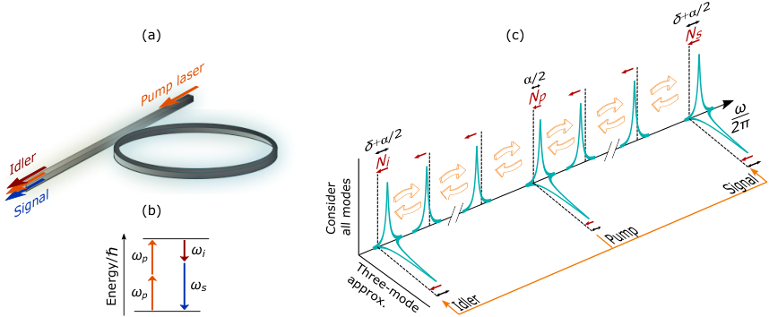
Recently, several experiments have been reported that advance the microresonator-based, degenerately-pumped OPO ($\mu$OPO) and make real headway towards a chip-scale, wavelength-by-design light source. Achievements include sub-milliwatt oscillation thresholds Lu et al. 2019, octave-spanning and tunable spectra Sayson et al. 2019; Tang et al. 2020, visible-light generation spanning red to green Lu et al. 2020; Domeneguetti et al. 2021, and a $\mu$OPO that uses a 2D photonic crystal cavity Marty et al. 2021. Nonetheless, the reported pump-to-signal conversion efficiencies are typically (except in instances involving narrow spectral bandwidths) $<0.1$% – a nonstarter for applications Lu et al. 2020; Sayson et al. 2019; Domeneguetti et al. 2021; Tang et al. 2020. Indeed, while the demand for efficiency calls for a deeper understanding of the underlying nonlinear physics, experiments have so far relied on a simplified theoretical framework for $\mu$OPOs. For instance, frequency matching is considered in either a cold-cavity limit Lu et al. 2019, or otherwise only accounts for a populated pump mode Sayson et al. 2019. A more accurate description of frequency matching should account for the exact distribution of intraresonator photons. Moreover, analyses have relied on a three-mode approximation (TMA), in which only the pump, signal, and idler modes interact through Kerr nonlinearity Sayson et al. 2019; Hansson et al. 2013. Of course, real microresonators comprise a more complex spectrum of modes that are nonlinearly coupled together. As a result, there is presently a gap between theoretical and experimental progress revolving around $\mu$OPOs; ultimately, there is little theoretical basis on which to design microresonators to meet end-user demands.

Here, we construct a generalized $\mu$OPO solution space; thereby, we reveal connections between the $\mu$OPO state and experimental parameters, and we identify processes that limit conversion efficiency. We adopt a model based on the Lugiato-Lefever Equation (LLE) Coen et al. 2013; Chembo and Menyuk 2013 and support our main numerical results with theoretical analyses. In the next section, we explain our modeling and present simulation results using a TMA. Then, we expand the model to include a spectrum of nonlinearly-coupled resonator modes. We demonstrate two nonlinear phenomena that cannot be explained within a TMA. In the first, a mode competition takes place between multiple signal and idler mode pairs. In the second, modulation instability induced by cross-phase modulation constrains the $\mu$OPO conversion efficiency. Finally, we propose two strategies for increasing the $\mu$OPO conversion efficiency and output power. Surprisingly, when comparing microresonators with different loss rates but identical geometries, we find that the resonator with greater losses will, in some cases, promote higher efficiency.

To study $\mu$OPOs, we consider a microring resonator coupled to an optical access waveguide and pumped by a continuous-wave (CW) laser, as depicted in Fig. 1a. This structure supports whispering gallery modes, in which azimuthal modes are grouped into families sharing a transverse spatial mode profile. Modes within a family are spaced (in the frequency domain) by a free-spectral range (FSR) that is inversely proportional to the ring circumference, $L$. In our model, we consider a single mode family and denote its resonant frequencies as $\omega_{\rm{\mu}}$, where $\mu$ is the azimuthal mode number shifted to make $\omega_{\rm{0}}$ the frequency of the pumped mode. The pump laser has frequency $\omega_{\rm{p}}$ and waveguide power $P_{\rm{in}}$, and the intraresonator field, $a$, obeys the Lugiato-Lefever Equation (LLE) Chembo and Menyuk 2013:

where $|a|^{2}$ gives the intraresonator energy in units of photon number, $\kappa_{\rm{c}}(\mu)$ is the mode-dependent coupling rate to the access waveguide, $\kappa_{\rm{i}}$ is the mode-independent intrinsic loss rate, $\kappa(\mu)=\kappa_{\rm{i}}+\kappa_{\rm{c}}(\mu)$ is the mode-dependent total loss rate, $\alpha=\frac{\omega_{\rm{0}}-\omega_{\rm{p}}}{\kappa(0)/2}$ is the normalized pump-resonator frequency detuning, $g_{\rm{0}}=\frac{n_{\rm{2}}c\hbar\omega_{\rm{0}}^{2}}{n^{2}V}$ is the nonlinear gain per photon, $n_{\rm{2}}$ is the Kerr index, $c$ is the speed of light in vacuum, $n$ is the refractive index, $V$ is the mode volume, and $\mathcal{D}(\mu)=\omega_{\rm{\mu}}-(\omega_{\rm{0}}+\mu D_{\rm{1}})+i\kappa_{\rm{c}}(\mu)$, where $D_{\rm{1}}=2\pi\times\textrm{FSR}$; $\tilde{a}$ indicates that operations to $a$ are performed in the frequency domain. Notably, the integrated dispersion, $D_{\rm{int}}$, is contained in Eq. 1 as $D_{\rm{int}}=Re(\mathcal{D})/\kappa(0)$. For concreteness, we use $n_{\rm{2}}=2.4\times 10^{-19}$ m²/W and $n=1.9$, which are typical values for silicon nitride (SiN) microrings, and $\omega_{\rm{p}}\approx 2\pi\times 384$ THz ($\approx$ 780 nm wavelength). Unless otherwise stated, we use $\kappa_{\rm{i}}=2\pi\times 200$ MHz and $\kappa_{\rm{c}}=\kappa_{\rm{i}}$ (i.e., critical coupling).

Figure 1c introduces some key concepts and illustrates differences between the TMA and the multi-mode LLE (here, ’multi-mode’ refers to the inclusion of many longitudinal modes from the same spatial mode family). The main difference is that a multi-mode model accounts for many more modes that can be coupled together by the Kerr nonlinearity. In contrast, a TMA only considers nonlinear interactions (e.g., FWM) between the pump, signal, and idler modes. Importantly, both models account for imperfect frequency matching. In general, phase-matched mode pairs (i.e., with azimuthal numbers $\pm\mu$) are not frequency matched – the associated FWM process does not conserve energy. Imperfect frequency matching is often quantified by the frequency mismatch parameter

Throughout, we use $\delta_{\rm{\mu}}$ to refer to the dispersive mismatch spectrum and $\delta$ to refer to the value of $\delta_{\rm{\mu(-\mu)}}$ at the targeted signal (idler) mode. A degenerate FWM process only conserves energy and momentum if $\delta$ is compensated by nonlinear frequency shifts of $\omega_{\rm{p(s,i)}}$, which we denote as $N_{\rm{p(s,i)}}$ for the pump (signal, idler) mode. Nonlinear shifts arise from self- and cross-phase modulation (SPM and XPM, respectively) and are related to the intraresonator intensity spectrum. Indeed, an occupied resonator necessarily implies $N_{p(s,i)}<0$; therefore, $\delta=0$ is not conducive to parametric oscillation.

Using a TMA, we investigate how changes in $\delta$ impact the $\mu$OPO, and then we introduce other modes into our simulations. To ensure the consistency of our numerical methods, we use the split-step Fourier method to simulate Eq. 1 for both the TMA and multi-mode LLE. Our primary goal is to understand the efficiency with which pump photons are converted into signal or idler photons. Accordingly, we define the conversion efficiency in units of photon flux as

where $\omega_{\rm{s(i)}}$ is the signal (idler) frequency and $P_{\rm{s(i)}}$ is the signal (idler) output power in the access waveguide. Importantly, the underlying symmetry of the FWM process implies that the signal and idler fields have equal $CE$ values and that $N_{\rm{s}}=N_{\rm{i}}$ for a critically-coupled resonator. Throughout, we present $CE$ for the signal; the same results apply to the idler.

In Fig. 2, we present simulation results obtained using a TMA. In a single simulation, $P_{\rm{in}}$ and $\delta$ are held fixed; we vary $\alpha$ to simulate a $\omega_{\rm{p}}$ scan across resonance from blue to red detuning, as shown in Fig. 2a. During the simulation, we record various data, including the $CE$, $N_{\rm{p(s,i)}}$, and optical spectra (see Supplemental Material for details). In Fig. 2a, each panel corresponds to $P_{\rm{in}}=20$ mW, but $\delta$ is increased from top to bottom. Our results indicate a highest obtainable $CE$ of $12.5$ % for critically-coupled resonators, in agreement with Ref. Sayson et al. 2019. Additionally, each panel depicts the effective signal detuning, defined as $\Delta_{\rm{s}}=\delta+\frac{\alpha}{2}-N_{\rm{s}}$. Notably, when $CE>0$, $\Delta_{\rm{s}}\approx 0$, which indicates that dispersion is perfectly compensated by detuning and nonlinearity in the $\mu$OPO state.

To fully characterize the relationship between $CE$, $P_{\rm{in}}$, and $\delta$, we construct the universal $CE$ map shown in Fig. 2b. The parameter space is defined by $P_{\rm{in}}$ and $\delta$; in Fig. 2b, we normalize $P_{\rm{in}}$ as

where $P_{\rm{th}}=\frac{\hbar\omega_{\rm{0}}\kappa^{3}(0)}{8g_{\rm{0}}\kappa_{\rm{c}}(0)}$ is the oscillation threshold power Kippenberg et al. 2004. Each data pixel in the $CE$ map represents the maximum $CE$ value taken from the corresponding LLE simulation, as indicated by the dashed line connecting Figs. 2a and 2b. The $CE$ map has a few notable features. First, we do not observe parametric oscillation for any values of $P_{\rm{in}}$ when $\delta\leq 0$. This indicates that nonlinear frequency shifts of $\omega_{\rm{\mu}}$ inhibit frequency matching even when $X\approx 1$. Second, $CE$ contours follow clear trends through the parameter space. In particular, to maintain $CE$ at larger values of $X$, $\delta$ must be increased, apparently to compensate for larger $N_{s(p,i)}$. Remarkably, we can derive an analytical expression for the contour of highest $CE$. We provide the derivation in the Supplemental Material; here, we present the final result, $X=8\delta$, and indicate it with the white dashed line in Fig. 2b. Clearly, to maximize $CE$ for a given $P_{\rm{in}}$, the microresonator dispersion (i.e., $\delta$) should be designed appropriately.

In Fig. 2a, it is perhaps remarkable that $CE$ values tend to increase monotonically until an abrupt cutoff. To elucidate this observation, we monitor the effective pump detuning, $\Delta_{\rm{p}}=\frac{\alpha}{2}-N_{\rm{p}}$, during our simulations and present a sample result in Fig. 2c. When $CE$ is greatest, $\Delta_{\rm{p}}$ reaches a minimum value near zero. Physically, this condition implies that $\omega_{\rm{p}}$ is nearly resonant; intuitively, this is necessary to maximize the dropped power and, in turn, the nonlinear gain. The cutoff results from Kerr bistability; i.e., when further increases in $\alpha$ are no longer compensated by $N_{\rm{p}}$, the intraresonator field abruptly transitions to the CW state. To characterize the universality of this feature, we record $\Delta_{\rm{p}}$ (evaluated for the highest $CE$) versus $\delta$ for two different powers, as shown in Fig. 2d. Apparently, realizing high $CE$ requires $\Delta_{\rm{p}}\approx 0$.

As a first step towards transitioning from a TMA to a multi-mode LLE, we briefly discuss the microresonator dispersion and its different representations. In Fig. 3a, we present $\delta_{\rm{\mu}}$ and $D_{\rm{int}}$ spectra for the fundamental transverse electric (TE) mode family, labeled TE1, of a SiN microring resonator (hereafter referred to as our test device) with ring radius $RR=15$ $\mu$m, ring width $RW=800$ nm, and height $H=600$ nm. We extract $\delta_{\rm{\mu}}$ and $D_{\rm{int}}$ from the mode spectrum, $\omega_{\rm{\mu}}$, that we calculate from finite-element method eigenfrequency simulations ¹¹ 1 Finite element simulations performed using Comsol Multiphysics, which is identified here to foster understanding, without implying recommendation or endorsement by NIST.. It is easy to show that $\delta_{\rm{\mu}}=2\times\mathcal{S}(D_{\rm{int}}(\mu))$, where $\mathcal{S}(D_{\rm{int}}(\mu))$ indicates the symmetric part of $D_{\rm{int}}$; i.e., the even orders of $D_{\rm{int}}$ when expressed as a Taylor expansion around $\mu=0$. We have assessed that analyzing $\delta_{\rm{\mu}}$ is sufficient to understand the $\mu$OPO dynamics, which are not sensitive to odd orders of $D_{\rm{int}}$ Sayson et al. 2019. This is a notable departure from other nonlinear microresonator eigenstates, e.g., dissipative Kerr solitons.

There are two defining features of the $\delta_{\rm{\mu}}$ spectrum shown in Fig. 3a. First, its negative curvature around $\mu=0$ indicates normal dispersion, which is required to suppress comb formation. Second, to overcome the normal dispersion and achieve frequency matching, the $D_{\rm{int}}$ expansion must contain higher order (even) terms such that $\delta_{\rm{\mu}}$ turns and becomes positive. Physically, this means that an anomalous-to-normal dispersion transition is necessary. Indeed, the dashed lines connecting Figs. 3a and 3b illustrate how $n_{\rm{g}}(\mu)=n_{\rm{g}}(-\mu)$ corresponds to a $\delta_{\rm{\mu}}$ turning point, where $n_{\rm{g}}(\mu)$ is the dispersive group velocity refractive index.

Next, we preview the differences between $CE$ maps calculated from multi-mode and TMA models. We observe two FWM processes, depicted in Fig. 4a, that require the multi-mode model. In one case, we observe mode competition between mode pairs with consecutive $\mu$ values. In the second case, we observe modulation instability (MI) in the normally-dispersive spectral region around $\omega_{\rm{p}}$, and we explain it as arising from XPM between the pump, signal, and idler fields. We mostly constrain our multi-mode LLE simulations to $P_{\rm{in}}\leq 25$ mW ($X\leq 8$); at higher values of $P_{\rm{in}}$, the $\mu$OPO dynamics become more complex.

Figure 4b shows a $CE$ map for our test device pumped near $\omega_{\rm{p}}=2\pi\times 382$ THz. To make a straightforward comparison between these data and Fig. 2b, we calculate the difference in $CE$ between the two $CE$ maps, as shown in Fig. 4c. In general, XPM-induced MI (XPM-MI) explains $CE$ differences for small $\delta$, while mode competition is responsible for the abrupt cutoff in $CE$ (marked by the sharp transition to zero $CE$ in Fig. 4b or the bold yellow stripe in Fig. 4c) that indicates a different mode pair is oscillating. In the following sections, we explore mode competition and XPM-MI in detail.

Mode competition is ubiquitous in laser systems with multi-mode resonators Narducci et al. 1986; Gong et al. 2007. In general, mode competition occurs when several resonator modes experience amplification simultaneously; hence, modes compete for gain and become coupled. In this section, we present the results of multi-mode LLE simulations in which several mode pairs are simultaneously nearly frequency matched. We use our findings to establish general principles for mode competition that will inform future microresonator designs.

In Fig. 5, we present simulation results for our test device pumped near $\omega_{\rm{p}}=2\pi\times 382$ THz. The FWM process related to mode competition is illustrated in Fig. 5a. Modes that are spectrally adjacent to the targeted signal and idler pair may be nearly frequency matched; hence, light in these modes may become amplified through FWM. To explore this phenomenon, we consider the $\delta_{\rm{\mu}}$ spectrum shown in Fig. 5b. According to the TMA, any mode pairs with $\delta_{\rm{\mu}}>0$ may oscillate, provided $P_{\rm{in}}$ is large enough. In Fig. 5b, the data points covered by the pale gold stripe indicate mode pairs that would oscillate when $P_{\rm{in}}=20$ mW, if they (along with the pump mode) were the only modes in the system (i.e., in a TMA). Hence, we endeavour to understand how a mode pair (or pairs) is chosen for oscillation over its spectral neighbors. To study mode competition in our test device, we perform multi-mode LLE simulations, from which we construct $CE$ maps for the modes corresponding to $\mu=46$, $\mu=45$, and $\mu=44$, as shown in Fig. 5c. To vary $\delta_{\rm{\mu}}$ (which is fixed for a given geometry), we apply a quadratic dispersion to $\omega_{\rm{\mu}}$, such that $\omega_{\rm{\mu}}\rightarrow\omega_{\rm{\mu}}+\beta\kappa(0)\mu^{2}$, where $\beta$ quantifies the added dispersion. We choose this approach in order to maintain the overall shape of $\delta_{\rm{\mu}}$. Note that $\delta_{\rm{45}}$ and $\delta_{\rm{44}}$ are both negative in Fig. 5b, but they will become positive as $\beta$ is increased.

The $CE$ maps in Fig. 5c present clear evidence for mode competition, and we identify three notable features in them. First, the $CE$ map for mode $\mu=46$ resembles that of the TMA for small $\delta_{\rm{46}}$. Second, as $\beta$ is increased, the maximum $CE$ for mode $\mu=46$ declines sharply, and this coincides with $\delta_{\rm{45}}>0$ and oscillation on mode $\mu=45$. This pattern repeats as $\beta$ is increased further – the oscillating mode changes from $\mu=45$ to $\mu=44$, and so on. Hence, we assess that the mode pair with smallest positive $\delta$ is favored for oscillation. Finally, there are small regions of parameter space where multiple mode pairs seem to oscillate simultaneously – we explore this phenomenon in Figs. 5d and 5e.

Figure 5d shows $CE$ for modes $\mu=46$ and $\mu=45$ during a $\omega_{\rm{p}}$ scan (i.e., varying $\alpha$) with $\beta=5\times 10^{-4}$ ($\delta_{\rm{46}}\approx 3$) and $P_{\rm{in}}=20$ mW. During the scan, mode $\mu=46$ begins to oscillate first; its $CE$ closely follows predictions made using a TMA (pale blue stripe) and reaches a maximum when $\alpha\approx 1.3$. In this regime, the $\mu$OPO spectrum is tri-modal, as depicted by the blue spectrum in Fig. 5e (the spectral bandwidth in Fig. 5e only spans $\omega_{\rm{p}}$ and $\omega_{\rm{s}}$; we have confirmed the spectrum is symmetric around $\omega_{\rm{p}}$). Beyond $\alpha\approx 1.3$, mode $\mu=45$ begins to oscillate, and $CE$ for mode $\mu=46$ deviates from its TMA counterpart. Between $\alpha\approx 1.3$ and $\alpha\approx 2.2$, both modes oscillate simultaneously, but their respective $CE$ values are not predicted by a TMA. Moreover, in this region the $\mu$OPO spectrum is not tri-modal; rather, it is strongly multi-moded with intensity peaks occurring near $\omega_{\rm{p}}$, $\omega_{\rm{s}}$, and $\omega_{\rm{i}}$, as shown by the orange spectrum in Fig. 5e. Beyond $\alpha\approx 2.2$, $CE$ for mode $\mu=46$ is zero, and $CE$ for mode $\mu=45$ follows its TMA counterpart. We term this phenomenon, wherein $CE$ values for different mode pairs conform to their TMA counterparts for different portions of a $\omega_{\rm{p}}$ scan, mode switching. Finally, at $\alpha\geq 3$, the $\mu$OPO decays in favor of MI. Remarkably, the MI state is supported in the normally-dispersive region around $\mu=0$ and without strong signal or idler fields. The MI spectrum is shown by the shaded red curve in Fig. 5e. In the next section, we explore MI and its impact on $CE$.

It is clear from Fig. 5 that mode competition is not the only process that differentiates the multi-mode LLE and TMA. Specifically, Figs. 5d and 5e establish that MI can suppress or extinguish the signal and idler fields, and this occurs in regions of parameter space where a TMA predicts efficient parametric oscillation. In this section, we isolate the MI process in our simulations by considering a special dispersion profile that eliminates mode competition, and we develop a theory for MI as arising from XPM between the pump, signal, and idler fields. We term this process XPM-MI to link it to previous investigations Agrawal 1987.

The XPM-MI FWM process is illustrated by the purple arrows in Fig. 6a. Energy from the pump laser is distributed to sidebands in a narrow spectral bandwidth around $\omega_{\rm{p}}$. If we use a multi-mode LLE to simulate our test device, the effects of mode competition can obfuscate the impact of XPM-MI. Therefore, we contrive the heuristically useful $\delta_{\rm{\mu}}$ spectra depicted in Fig. 6b. Here, we define $\delta_{\rm{\mu}}=-2\beta\mu^{2}$ for all $\mu\neq\pm 50$. The modes $\mu=\pm 50$ are designated for parametric oscillation and assigned a frequency mismatch value $\delta$ that can be manipulated apart from $\beta$.

In Fig. 6c, we present LLE simulations of $CE$ versus $\alpha$ for microresonators with the $\delta_{\rm{\mu}}$ spectra in Fig. 6b; these data overlay the corresponding simulation using a TMA (pale gray stripe). They are representative of the entire ($P_{\rm{in}},\delta)$ parameter space, and they are noteworthy for two reasons. First, in all cases $CE$ follows the gray stripe until $\alpha\geq\alpha_{\rm{ON}}$, where $\alpha_{\rm{ON}}$ corresponds to the onset of XPM-MI. An example XPM-MI spectrum is shown in Fig. 6d. Unlike the XPM-MI spectrum shown in Fig. 5e, here the XPM-MI and $\mu$OPO states co-exist, albeit with suppressed $CE$. Second, $\alpha_{\rm{ON}}$ increases with increasing $\beta$. As a result, $CE$ fully converges to its TMA counterpart in the high-$\beta$ limit. To investigate this convergence, we construct the $CE$ maps for different values of $\beta$, and we present the results in Fig. 6e. We observe steady convergence to the TMA $CE$ map as $\beta$ is increased. Clearly, it is crucial to realize strong normal dispersion near $\omega_{\rm{p}}$ to observe efficient parametric oscillation when $X>>1$.

Next, we present an expression for the XPM-MI gain that we derive from a set of coupled mode equations (see Supplemental Material for details), and we analyze this expression to support our conclusion that XPM underlies the observed MI states. As noted in Ref. Hansson et al. 2013, MI may occur in normally-dispersive microresonators; however, it usually requires a hard excitation, i.e., the MI sidebands are not amplified from vacuum fluctuations. This fact explains how the MI state can sometimes persist after parametric oscillations decay. Still, in our simulations we have never observed MI emerge before parametric oscillations. Indeed, it was predicted in Ref. Agrawal 1987 that XPM between two waves can make them modulationally unstable, even when one or both waves propagates in normally-dispersive media. Motivated by this study, we analyze a set of coupled mode equations that assume the pump, signal, and idler modes are occupied, and we derive the MI gain, $\lambda_{\rm{\mu}}$, as

where $I_{\rm{0}}$ and $I_{\rm{s}}$ are the photon numbers for the pump and signal modes, respectively, $\Delta\phi=2\phi_{\rm{p}}-\phi_{\rm{s}}-\phi_{\rm{i}}$ is the relative phase mismatch between the pump, signal, and idler fields, which are expressed as $\tilde{a}_{\rm{p(s,i)}}=\sqrt{I_{\rm{p(s,i)}}}e^{-i\phi_{\rm{p(s,i)}}}$, and $k_{\rm{\mu}}=2I_{\rm{0}}+4I_{\rm{s}}-\beta\mu^{2}-\alpha$. MI occurs when $\lambda_{\rm{\mu}}>0$, for any $\mu$. Note from these definitions that $\beta\mu^{2}$ is the frequency mismatch parameter for the MI sidebands, with mode numbers $\pm\mu$, and not the frequency mismatch for the $\mu$OPO mode pair, which we denote as $\delta$. In the limit $I_{\rm{s}}\rightarrow 0$, Eq. 5 is equivalent to the MI gain expression derived in Ref. Hansson et al. 2013. Moreover, it is clear that $\lambda_{\rm{\mu}}$ is maximized when the pump, signal, and idler fields are in phase (i.e. when $\Delta\phi=0$), which corresponds to the in-phase addition of two FWM processes: the degenerate FWM process $2\omega_{\rm{p}}\rightarrow\omega_{\rm{\mu}}+\omega_{\rm{-\mu}}$ and the non-degenerate process $\omega_{\rm{s}}+\omega_{\rm{i}}\rightarrow\omega_{\rm{\mu}}+\omega_{\rm{-\mu}}$.

To analyze XPM-MI using Eq. 5, we perform LLE simulations, using a TMA, for various values of $P_{\rm{in}}$ and $\delta$ and extract values for $I_{\rm{0}},I_{\rm{s}}$, and $\Delta\phi$ that we use to calculate $\lambda_{\rm{\mu}}$. When $\lambda_{\rm{\mu}}>0$, the mode pair with mode numbers $\pm\mu$ will be amplified and steal energy from the $\mu$OPO. In general, a large normal dispersion leads to the sideband pair with $\mu=\pm 1$ having the largest gain; therefore, in what follows we drop the $\mu$ subscript and define $\lambda$ as the MI gain for this pair. We have confirmed that $\lambda_{\rm{\mu}}<0$ whenever $I_{\rm{s}}=0$ and $\beta>0$; physically, this means that XPM between the pump, sigal, and idler fields is required to initiate MI for microresonators with normal dispersion. Hence, we term this process XPM-MI. Figure 7a presents $\lambda$ calculations for various values of $P_{\rm{in}}$, $\delta$, and $\beta$. They indicate that $\lambda$ grows with increasing $\alpha$, which is explained by the stronger XPM that results from more powerful $\mu$OPO sidebands at large $\alpha$. To compare our XPM-MI theory (i.e., Eq. 5) to multi-mode LLE simulations, we calculate $\alpha_{\rm{ON}}$ in both cases, for different values of $\beta$. Overall, we observe good agreement, but Eq. 5 generally predicts higher values of $\alpha_{\rm{ON}}$ than the multi-mode LLE. A sample comparison of this type is presented in Fig. 7b.

To more comprehensively compare our theory with multi-mode LLE simulations, we calculate the maximum gain, $\lambda_{\rm{max}}$, for $\beta=0.25$ and different values of $P_{\rm{in}}$ and $\delta$. We use these data to construct the $\lambda_{\rm{max}}$ map presented in Fig. 7c. It accurately predicts the threshold $P_{\rm{in}}$ values for XPM-MI, and it has the overall trend that $\lambda_{\rm{max}}$ grows with increasing $P_{\rm{in}}$ and $\delta$. This trend is consistent with the $CE$ maps presented in Fig. 6e, which deviate from the TMA as $P_{\rm{in}}$ and $\delta$ are increased. Importantly, our observations may explain prior experimental results, which consistently report that increasing $P_{\rm{in}}$ leads to the formation of undesired sidebands Lu et al. 2019; Tang et al. 2020; Fujii et al. 2019. Overall, our theory supports the hypothesis that XPM drives MI in a $\mu$OPO. Moreover, we can now form a concise description of parasitic FWM in $\mu$OPOs: Mode competition dictates which mode pair oscillates, while XPM-MI constrains $CE$.

Our results suggest several design rules for avoiding mode competition and mitigating XPM-MI through dispersion engineering. For example, Fig. 6 demonstrates that larger normal dispersion around $\omega_{\rm{p}}$ will suppress XPM-MI. Moreover, increasing $\frac{d\delta_{\rm{\mu}}}{d\mu}$ will help prevent mode competitions. This can be accomplished by using smaller resonators or in resonators with greater dispersion. Still, in practice it is nontrivial to fabricate devices with ideal dispersion characteristics. Therefore, in this section we describe two strategies to increase $CE$ by tuning the microresonator loss rates, $\kappa_{\rm{c}}(\mu)$ and $\kappa_{\rm{i}}$. We assume that users of real-world $\mu$OPO devices will value high output power; therefore, we focus on ways to increase $CE$ for fixed $P_{\rm{in}}$.

Figure 8a depicts the coupling and intrinsic loss rates that are quantified by $\kappa_{\rm{c}}(\mu)$ and $\kappa_{\rm{i}}$, respectively. In practice, $\kappa_{\rm{c}}(\mu)$ is controllable by various design parameters, including the waveguide-resonator separation and waveguide-resonator coupling length, for example, in a ‘pulley’ configuration  Moille et al. 2019. Moreover, $\kappa_{\rm{i}}$ can be reduced within some spectral bands by annealing Spencer et al. 2014; Graziosi et al. 2018; hence, one gains some control over $\kappa_{\rm{i}}$ by making a suitable choice for the annealing time or temperature (also, increasing $\kappa_{\rm{i}}$ can be realized through, for example, intentionally-introduced surface roughness).

We consider two ways to increase $CE$. First, by increasing $P_{\rm{th}}$, one increases the $P_{\rm{in}}$ values for which XPM-MI occurs. To demonstrate this approach, we perform multi-mode LLE simulations of our test device for three different values of $\kappa$. In every simulation, $\kappa_{\rm{c}}(\mu)=\kappa_{\rm{i}}$ and $\omega_{\rm{p}}=2\pi\times 385$ THz. The simulated modal lineshapes for these resonators are shown in Fig. 8b, and the corresponding $CE$ maps are shown in Fig. 8c. In Fig. 8c, $\kappa$ is increased from the left-most panel to the right-most panel. As $\kappa$ is increased, the region of highest $CE$ is shifted towards higher values of $P_{\rm{in}}$. Moreover, this region is broadened along both axes, indicating that devices with larger $\kappa$ will have a greater tolerance for design errors in $\delta$. While increases in $\kappa$ prevent high $CE$ at low $P_{\rm{in}}$, the obtainable output power generated with high $P_{\rm{in}}$ has grown; for instance, with $P_{\rm{in}}=30$ mW, the maximum output power increases from $P_{\rm{sig}}\approx 2.25$ mW at $\kappa/2\pi=250$ MHz (Fig. 8c, left-most panel) to $P_{\rm{sig}}\approx 3.75$ mW at $\kappa/2\pi=550$ MHz (Fig. 8c, right-most panel).

Finally, we consider the relationship between the signal mode coupling rate, $\kappa_{\rm{c}}$, and $CE$. This relationship was explored in Ref. Sayson et al. 2019, with the result that $CE$ may be as large as $25$% (overcoupling the pump mode may further increase $CE$). Here, we reiterate this result and explore it within the $\mu$OPO parameter space. Figure 8d shows simulated signal mode lineshapes for two values of $\kappa_{\rm{c}}$, and Fig. 8e shows the $CE$ map for $P_{\rm{in}}=20$ mW in a parameter space defined by the coupling ratio, $\kappa_{\rm{c}}/\kappa_{\rm{i}}$, and $\delta$. In our simulations, we use a TMA and keep the pump and idler modes critically coupled. We not only observe an increase in the highest obtainable $CE$ to nearly $25$%, but we also observe that the region of highest $CE$ is broadened for increasing $\kappa_{\rm{c}}/\kappa_{\rm{i}}$. Broadening occurs until $\kappa_{\rm{c}}/\kappa_{\rm{i}}\approx 30$, at which point the advantages of overcoupling are overcome by the corresponding increases in $P_{\rm{th}}$.

In conclusion, we have established a foundation of simulation results for $\mu$OPOs that moves beyond a TMA and will help guide experimental efforts to realize the high conversion efficiencies predicted by the simplified theory. We introduced a $CE$ map that encapsulates the $\mu$OPO solution space, and through multi-mode LLE simulations we reveal nonlinear dynamics not predictable from a TMA. In particular, we identified mode competition and demonstrated how it determines the oscillating mode pair. Meanwhile, the range of parameter space over which high $CE$ can be obtained is constrained by XPM-MI. Mode competition and XPM-MI both depend on the microresonator dispersion, $\delta_{\rm{\mu}}$, and suitable dispersion engineering may circumvent these processes. Still, optimizing $\delta_{\rm{\mu}}$ may be nontrivial in practice; therefore, we have proposed two strategies to increase $CE$ apart from dispersion engineering. Ultimately, suitable control of both resonator loss (including waveguide coupling) and dispersion makes it possible to tailor microresonator geometries for high $CE$ at a targeted pump power, that is, to produce a useful amount of output power. Such engineering will be crucial in the development of compact, coherent light sources that take advantage of the enormous wavelength flexibility inherent to $\chi^{(3)}$ OPOs.

Supplemental Material

In this section, we describe mathematical formulae that relate LLE variables to the data (e.g. $CE$ and optical spectra) presented in the main text. Simulations of the Lugiato-Lefever Equation (LLE) yield solutions for the complex intraresonator field, $a$; we denote the intraresonator field spectrum $\tilde{a}=\mathcal{F}(a)$, where $\mathcal{F}$ denotes the Fourier transform, and $a$ is normalized such that $|\tilde{a}|^{2}_{\omega=\omega_{\mu}}$ gives the number of intraresonator photons in the mode $\mu$.

Table 1 lists the important variables, along with their physical descriptions and how they are calculated from $a$, $\tilde{a}$, and simulation parameters. Notably, the expressions for $\phi_{\rm{p}}$ and $N_{\rm{p}}$ also apply to the signal and idler modes when the expressions are evaluated at the appropriate value of $\omega$. We follow Ref. Yu et al. 2021 in our calculation of the nonlinear mode frequency shifts.

Next, we seek to derive the result - stated in the main text - that the contour of highest maximum $CE$ in the TMA is given by $X=8\delta$. Our starting point is the following set of coupled equations Sayson et al. 2019:

where $A_{\rm{p(s,i)}}=\sqrt{I_{\rm{p(s,i)}}}e^{-i\phi_{\rm{p(s,i)}}}$ denotes the pump (signal, idler) field, and $I_{\rm{p(s,i)}}=|A_{\rm{p(s,i)}}|^{2}$ is proportional to the pump (signal, idler) intraresonator photon number. If we substitute the field expressions into the above equations, we obtain six coupled equations for the real variables $I_{\rm{p(s,i)}}$ and $\phi_{\rm{p(s,i)}}$,

where $\Delta\phi=2\phi_{\rm{p}}-\phi_{\rm{s}}-\phi_{\rm{i}}$. We next reduce this system to four equations by first noting that, from the symmetry of Eqs. 7 and 8, $I_{\rm{s}}=I_{\rm{i}}$. Therefore, we define $M=I_{\rm{s}}=I_{\rm{i}}$. Moreover, momentum conservation implies that $\frac{d}{dt}(\phi_{\rm{s}}+\phi_{\rm{i}})=0$. Hence, for steady state conditions we obtain

Equations 15-18 are still sufficiently general to study the stationary solutions. However, we proceed to simplify them via two ansatzes associated with a maximally efficient $\mu$OPO. Specifically, we set $\phi_{\rm{p}}=0$, which corresponds to the pump laser being on resonance, and $M=\frac{I_{\rm{p}}}{2}$. The validity of these assumptions is confirmed by our numerical results, but they are also physically intuitive. For instance, because the FWM process that drives $\mu$OPO ($2\omega_{\rm{p}}\rightarrow\omega_{\rm{s}}+\omega_{\rm{i}}$) is reversible, one expects the intraresonator photons to be evenly distributed between the pump mode and sideband pair.

After inserting our two ansatzes into Eqs. 15-18, we combine Eqs. 15 and 16 to obtain $I_{\rm{p}}=X/4$. Then, Eqs. 17 and 18 are combined to obtain $\frac{I_{\rm{p}}}{2}=\delta$. Insertion of the former into the latter yields the desired result, $X=8\delta$.

Finally, in this section we derive Eq. 4 from the main text. We follow the classical procedure of linearizing a set of coupled equations around a steady-state solution and then allowing plane-wave perturbations to grow exponentially. We start from the equations of motion for the fields $A_{\rm{\mu}}$ and $A_{\rm{-\mu}}$ when the pump, signal, and idler modes are occupied,

where $\beta$ quantifies the dispersion. Next, we introduce the perturbation $\delta f_{\rm{\mu}}(t)$, so that the equations of motion for the perturbations, after simplifying, read

where $k_{\rm{\mu}}=\beta\mu^{2}+2I_{\rm{p}}+4I_{\rm{s}}-\alpha$, and we have again assumed $I_{\rm{s}}=I_{\rm{i}}$. If we set $\delta f_{\rm{\mu}}(t)=ae^{\lambda_{\rm{\mu}}t}$, then we obtain a set of linear homogenous equations with eigenvalue $\lambda_{\rm{\mu}}$. Solving the eigenvalue problem yields

which is the desired result. Notably, the original set of coupled equations are approximations in several ways. For instance, we only consider one sideband pair, but the full XPM-MI dynamics involves the collective interactions of multiple sideband pairs simultaneously. In addition, we neglect FWM processes that do not involve both MI sidebands (e.g. the interaction $A_{\rm{\mu}}^{*}A_{\rm{s}}^{*}A_{\rm{p}}A_{\rm{s+\mu}}$). These approximations may explain the small discrepancies between our theory and LLE simulations.

References

- Liang and Bowers (2010) D. Liang and J. E. Bowers, Nature Photonics 4, 511 (2010).
- Agrell et al. (2016) E. Agrell, M. Karlsson, A. Chraplyvy, D. J. Richardson, P. M. Krummrich, P. Winzer, K. Roberts, J. K. Fischer, S. J. Savory, B. J. Eggleton, et al., Journal of Optics 18, 063002 (2016).
- Sipahigil et al. (2016) A. Sipahigil, R. E. Evans, D. D. Sukachev, M. J. Burek, J. Borregaard, M. K. Bhaskar, C. T. Nguyen, J. L. Pacheco, H. A. Atikian, C. Meuwly, et al., Science 354, 847 (2016).
- Elshaari et al. (2020) A. W. Elshaari, W. Pernice, K. Srinivasan, O. Benson, and V. Zwiller, Nature Photonics 14, 285 (2020).
- Jin et al. (2021) W. Jin, Q.-F. Yang, L. Chang, B. Shen, H. Wang, M. A. Leal, L. Wu, M. Gao, A. Feshali, M. Paniccia, et al., Nature Photonics 15, 346 (2021).
- Vahala (2003) K. J. Vahala, Nature 424, 839 (2003).
- Yang et al. (2018) K. Y. Yang, D. Y. Oh, S. H. Lee, Q.-F. Yang, X. Yi, B. Shen, H. Wang, and K. Vahala, Nature Photonics 12, 297 (2018).
- Kippenberg et al. (2018) T. J. Kippenberg, A. L. Gaeta, M. Lipson, and M. L. Gorodetsky, Science 361 (2018).
- Liu et al. (2018) X. Liu, C. Sun, B. Xiong, L. Wang, J. Wang, Y. Han, Z. Hao, H. Li, Y. Luo, J. Yan, et al., ACS Photonics 5, 1943 (2018).
- Loh et al. (2015) W. Loh, A. A. Green, F. N. Baynes, D. C. Cole, F. J. Quinlan, H. Lee, K. J. Vahala, S. B. Papp, and S. A. Diddams, Optica 2, 225 (2015).
- Bruch et al. (2019) A. W. Bruch, X. Liu, J. B. Surya, C.-L. Zou, and H. X. Tang, Optica 6, 1361 (2019).
- Lu et al. (2019) X. Lu, G. Moille, A. Singh, Q. Li, D. A. Westly, A. Rao, S.-P. Yu, T. C. Briles, S. B. Papp, and K. Srinivasan, Optica 6, 1535 (2019).
- Spencer et al. (2018) D. T. Spencer, T. Drake, T. C. Briles, J. Stone, L. C. Sinclair, C. Fredrick, Q. Li, D. Westly, B. R. Ilic, A. Bluestone, et al., Nature 557, 81 (2018).
- Marin-Palomo et al. (2017) P. Marin-Palomo, J. N. Kemal, M. Karpov, A. Kordts, J. Pfeifle, M. H. Pfeiffer, P. Trocha, S. Wolf, V. Brasch, M. H. Anderson, et al., Nature 546, 274 (2017).
- Lai et al. (2020) Y.-H. Lai, M.-G. Suh, Y.-K. Lu, B. Shen, Q.-F. Yang, H. Wang, J. Li, S. H. Lee, K. Y. Yang, and K. Vahala, Nature Photonics 14, 345 (2020).
- Newman et al. (2019) Z. L. Newman, V. Maurice, T. Drake, J. R. Stone, T. C. Briles, D. T. Spencer, C. Fredrick, Q. Li, D. Westly, B. R. Ilic, et al., Optica 6, 680 (2019).
- Vodopyanov et al. (2000) K. Vodopyanov, F. Ganikhanov, J. Maffetone, I. Zwieback, and W. Ruderman, Optics Letters 25, 841 (2000).
- Mieth et al. (2014) S. Mieth, A. Henderson, and T. Halfmann, Optics express 22, 11182 (2014).
- Boyd (2020) R. W. Boyd, Nonlinear optics (Academic press, 2020).
- Lu and Srinivasan (2021) X. Lu and K. Srinivasan, Physical Review Applied 16, 014027 (2021).
- Sayson et al. (2019) N. L. B. Sayson, T. Bi, V. Ng, H. Pham, L. S. Trainor, H. G. Schwefel, S. Coen, M. Erkintalo, and S. G. Murdoch, Nature Photonics 13, 701 (2019).
- Tang et al. (2020) Y. Tang, Z. Gong, X. Liu, and H. X. Tang, Optics Letters 45, 1124 (2020).
- Lu et al. (2020) X. Lu, G. Moille, A. Rao, D. A. Westly, and K. Srinivasan, Optica 7, 1417 (2020).
- Domeneguetti et al. (2021) R. R. Domeneguetti, Y. Zhao, X. Ji, M. Martinelli, M. Lipson, A. L. Gaeta, and P. Nussenzveig, Optica 8, 316 (2021).
- Marty et al. (2021) G. Marty, S. Combrié, F. Raineri, and A. De Rossi, Nature Photonics 15, 53 (2021).
- Hansson et al. (2013) T. Hansson, D. Modotto, and S. Wabnitz, Physical Review A 88, 023819 (2013).
- Coen et al. (2013) S. Coen, H. G. Randle, T. Sylvestre, and M. Erkintalo, Optics Letters 38, 37 (2013).
- Chembo and Menyuk (2013) Y. K. Chembo and C. R. Menyuk, Physical Review A 87, 053852 (2013).
- Kippenberg et al. (2004) T. Kippenberg, S. Spillane, and K. Vahala, Physical review letters 93, 083904 (2004).
- (30) Finite element simulations performed using Comsol Multiphysics, which is identified here to foster understanding, without implying recommendation or endorsement by NIST.
- Narducci et al. (1986) L. Narducci, J. Tredicce, L. Lugiato, N. Abraham, and D. Bandy, Physical Review A 33, 1842 (1986).
- Gong et al. (2007) M. Gong, Y. Yuan, C. Li, P. Yan, H. Zhang, and S. Liao, Optics Express 15, 3236 (2007).
- Agrawal (1987) G. P. Agrawal, Physical Review Letters 59, 880 (1987).
- Fujii et al. (2019) S. Fujii, S. Tanaka, M. Fuchida, H. Amano, Y. Hayama, R. Suzuki, Y. Kakinuma, and T. Tanabe, Optics letters 44, 3146 (2019).
- Moille et al. (2019) G. Moille, Q. Li, T. C. Briles, S.-P. Yu, T. Drake, X. Lu, A. Rao, D. Westly, S. B. Papp, and K. Srinivasan, Optics Letters 44, 4737 (2019).
- Spencer et al. (2014) D. T. Spencer, J. F. Bauters, M. J. Heck, and J. E. Bowers, Optica 1, 153 (2014).
- Graziosi et al. (2018) T. Graziosi, S. Mi, M. Kiss, and N. Quack, in 2018 International Conference on Optical MEMS and Nanophotonics (OMN) (IEEE, 2018) pp. 1–5.
- Yu et al. (2021) S.-P. Yu, D. C. Cole, H. Jung, G. T. Moille, K. Srinivasan, and S. B. Papp, Nature Photonics 15, 461 (2021).