Interference effect of beam splitter current in Iron-Pnictide superconductorsPreprint: APS/123-QED

One of the fundamental aspect of quantum mechanics is the superposition principle which dictates that a quantum mechanical system can be described by a linear superposition of many orthogonal wave functions sakurai. This superposition principle yields an entanglement or correlations between different parts of the system. In recent times this fundamental aspect has been investigated in detail to construct entangled states having specific properties with application in teleportation, cryptology etc neilson. To realize such entangled states many protocols have been proposed involving various mesoscopic system such as quantum dots, superconducting qubits etc divincenzo; djordjevic; gaard; montanaro. However after preparing such entangled state one needs to confirm that the state is robust against decoherence decoher1; decoher2. It is well known fact that various condensed matter system act as a source of such entangled many body states naturally. The existence of such entangled states is ubiquitous in various condensed matter systems such as the Cooper pairs in superconductivity tinkham, ground state wave-function for quantum spin liquid spinliq1; spinliq2, resonating valence bond states baskaran for certain magnetic systems etc.

In FeAs, the relevant tight binding model which describes the superconductivity contains an itinerant electron system of two electronic orbitals due to two Fe atoms in an unit cell araujo; bang; hu-ting-zhu; jiang-li-wang. The hybridization between the orbitals are such that it leads to a hole pocket centred at $(0,0)$ and an electron pocket centred at $(\pi,\pi)$ in the folded zone scheme chubukov1; chubukov2. Following earlier notationschubukov1 we denote the fermions near $(0,0)$ by usual ‘$c$’ operator and for fermions near $(\pi,\pi)$ by ‘$f$’. The model Hamiltonian can be written as follows,

In the above $H_{0}$ denotes the non-interacting part of electron and hole pocket. $H_{\Delta}$ denotes superconducting pairing interaction and $H_{m}$ signifies the magnetic pairing interaction. The details of these three terms are given below chubukov2,

In the above $\epsilon_{c}=\mu_{c}-|k|^{2}/2m$ and $\epsilon_{f}=|k^{\prime}|^{2}/2m-\mu_{f}$. Note that $k$ appearing in ‘$c$’ is measured from the center of Brillouine zone and for ‘$f$’ fermion $k^{\prime}$ is measured from ($\pi,\pi$). Henceforth all the momentum indices associated with the ’$f$’ fermions are understood as measured from ($\pi,\pi$) unless referred otherwise. Note that we have taken an isotropic mass at electron pocket and hole pocket. This assumption may be an approximated one without changing the qualitative aspect of the results found here. The superconducting pairing terms and the magnetic interactions are given by,

Where $\delta p=p^{\prime}-p$ and $\delta k=k^{\prime}-k$ and $[\Lambda]=\alpha\beta\beta^{\prime}\alpha^{\prime}$ denotes combined spin indices. In the above, Eq. 3 describes the effective pairing interactions in the Iron-pnictide system which arises due to the inter-band hopping between electron and hole band chubukov1. The magnetic interactions as denoted in Eq. 4 come from the inter-band density-density interactions. The pairing interaction $V_{\alpha\beta\beta^{\prime}\alpha^{\prime}}^{cf}(k,p)=V_{k,p}^{sc}((i\sigma^{y})_{\alpha\beta}(i\sigma^{y})^{+}_{\beta^{\prime}\alpha^{\prime}}$ and the magnetic interaction $V_{\alpha\beta\beta^{\prime}\alpha^{\prime}}^{sw}(p^{\prime}p:kk^{\prime})=V_{p^{\prime}p:kk^{\prime}}^{sw}\bm{\sigma}_{\alpha\beta}.\bm{\sigma}_{\beta^{\prime}\alpha^{\prime}}^{+}$. Following earlier convention chubukov1; chubukov2, we define the superconducting pairing order parameter and magnetic order parameter as $\Delta_{c}(k)_{\alpha\beta}=(i\sigma^{y})_{\alpha\beta}\sum_{p}V_{kp}^{sc}(i\sigma^{y})_{\beta^{\prime}\alpha^{\prime}}^{+}\langle f_{-p\beta^{\prime}}f_{p\alpha^{\prime}}\rangle,(m_{q})_{\alpha\beta}=-\frac{V^{sw}}{2}\sum_{p}\bm{\sigma_{\alpha\beta}}.\bm{\sigma_{\beta^{\prime}\alpha^{\prime}}^{+}}\langle c_{p\beta^{\prime}}^{+}f_{p+q\alpha^{\prime}}\rangle$. $\Delta_{f}(k)_{\alpha,\beta}$ is defined identically as $\Delta_{c}(k){\alpha,\beta}$. Note that the momentum index $q$ appearing in the definition of magnetic order parameter $m_{q}$ refers a small deviation of the centre of hole pocket from ($\pi,\pi$). This is to account for the fact that when $q=0$, magnetic order is found to be zero which will be discussed again Sec. IV. We use the above definitions of mean field order parameters to perform a meanfield decomposition of the four fermion interactions as given in Eq. 3 and Eq. 4. The resulting Hamiltonian obtained is written in the following matrix form,

where the four component Nambu spinor is, $\overline{\Psi}_{k\alpha}=(c_{k\alpha}^{+},c_{-k\alpha},f_{p\alpha}^{+},f_{-p\alpha})$ with $p=k+q$ and the Hamiltonian matrix $\hat{\mathcal{H}}(k)_{\alpha\beta}$ which we write in short $\hat{\mathcal{H}}_{\alpha\beta}$ has the form,

Note that initially the superconducting pairing interaction (as given in Eq. 3) is defined such a way that a hole of momenta $k$ can interact with another electron of momenta $p$ belonging to electron pocket centred around $(\pi,-\pi)$. However in the final expression in Eq. 5 another simplification has been performed where a hole with momenta $k$ take part in pairing interaction with another electron at hole pocket with momenta $k$ only. The index $q$ signifies that the electron pocket is no longer around $(\pi,-\pi)$ but rather around $(\pi,-\pi)+q$ to take into account finite magnetic order parameter. In the above we have accounted for two different kind of magnetic order parameter with the following definitions. If $\alpha=\beta,m_{\alpha,\alpha}=m_{1}$ and for $\alpha\neq\beta,~~m_{2}=m_{\alpha,\beta}$. Following earlier study chubukov1; chubukov2 we choose $m_{1}=m,m_{2}=0$ in our study without loss of generality. One can easily obtain the spectrum after diagonalizing the $8\times 8$ matrix in Eq. 6, the detail expressions for the eigenvalues are given in Appendix B. We obtain the ground state energy by filling the negative energy eigenstates which correspond to the vacuum of new Bogoliubov quasi-particles. Along with the constant terms the ground state energy can be written as $E_{min}=-\mathcal{E}_{kq+}-\mathcal{E}_{kq-}-\frac{\Delta_{c}\Delta_{f}}{V_{SC}}+2\frac{m^{2}}{V_{SD}}$. Where $\mathcal{E}_{kq\pm}=\sqrt{\mathcal{P}_{k}\pm\sqrt{\mathcal{Q}_{k}}}$ where $\mathcal{P}_{k}$ and $\mathcal{Q}_{k}$ are functional of $\epsilon_{c}(k),\epsilon_{f}(p),\Delta_{c},\Delta_{f},m$ and their detail expressions are given in Appendix B. We first derive the self consistent equations for the meanfield order parameter by minimizing Eq. 5 with respect to appropriate meanfield order parameters. Next we evaluate those meanfield order parameters self-consistently with the help of eigenvectors obtained after diagonalizing Eq. 6. Once the meanfield order parameters values are obtained we use them to calculate the beam-splitter current. Note that we evaluate the meanfield order parameters at zero temperature and thus beam-splitter current refers to zero temperature study only. Now we move on briefly to describe the beam-splitter current calculation.

Having described the basic model of superconductivity and coexistence of magnetic order with it in Iron-Pnictides we now elaborate on the beam splitter arrangement designed for such system. Our idea of entangled Cooper pair splitter is similar to the seminal work of daniel where for the first time an outline of Cooper pair entangled beam splitter arrangement was introduced. In Fig. 2, we present a schematic diagram of entangled beam-splitter arrangement. It is expected that electrons in a superconducting Copper pair in an iron-pnictide material will be tunneling through two spatially separated quantum dots where each quantum dot allows one electron (among the two participating electrons in a superconducting pair). However we note that in previous studies daniel; firoz a superconducting eigenstate is of the form $\gamma_{k}=u_{k}c_{\uparrow,k}+v_{k}c^{\dagger}_{\downarrow,-k}$ and hence there are possibilities of only two kind of currents. The first one is where the electron with spin up and momentum $k$ enters into one of the quantum dot and the other enters into the remaining quantum dot. This current is defined as $\mathcal{I}_{1}$ and it shows characteristic oscillations with the separation between the quantum dots. The second kind of current is obtained where both the electrons enter through the same dot with some time gap in between them. This current is defined as $\mathcal{I}_{2}$ and it is found to be a constant for a given set of parameters. The ratio $\mathcal{I}_{1}/\mathcal{I}_{2}$ signifies the efficiency of the beam splitter current so as to differentiate the $\mathcal{I}_{1}$ from $\mathcal{I}_{2}$. In the present scannerio an eigenstate in superconducting phase is of the form $\gamma^{\prime}_{k}=u_{k}c_{\uparrow,k}+v_{k}c^{\dagger}_{\downarrow,-k}+u^{\prime}_{k}f_{\uparrow,k}+v^{\prime}_{p}f^{\dagger}_{\downarrow,-p}$. Hence in our case the current $\mathcal{I}_{1}$ is obtained by considering the two participating entangled Cooper pair, one due to $c$-fermion and another due to $f$-fermion. Note that we do not consider the current due to tunneling of a $c$ and $f$ fermion which participate in magnetic ordering. The current due to such event vanishes due to singlet nature of the quantum dot and metallic lead.

The current $\mathcal{I}_{1}$ is expected to happen once the quantum dots are kept in the Coulomb blockade regime such that it is energetically unfavorable to accommodate two electrons at the same quantum dot. Finally once two spatially separated electrons enter into two separate quantum dots, they are collected by two fermi liquid leads (represented by L₁ and L₂ in Fig. 2). However to realize such entangled electrons to be separated the chemical potentials of the superconducting materials ($\mu_{s}$), quantum dots($\epsilon_{1}$ and $\epsilon_{2}$) and also the leads($\mu_{1}$ and $\mu_{2}$) are to be kept in certain conditions. While the chemical potentials at the two fermi liquid leads can be kept equal generally, the chemical potentials of the two quantum dots should be such that $\epsilon_{1}+\epsilon_{2}=2\mu_{s}$ corresponding to two particle Breit-Wigner resonance Sumetski. The transport of two entangled electron or hole pairs from the quantum dots to the leads can be achieved by applying a bias voltage $\Delta\mu=\mu_{s}-\mu_{l}$. We here outline the calculation of $\mathcal{I}_{1}$ and the details about $\mathcal{I}_{2}$ is discussed in Sec. V and in Appendix-A.
It is natural to expect that once the electrons tunnel from the superconductor to quantum dots, they interact with the already existing electrons at the quantum dots and this might lead to decoherence between the two separated electrons. One way to avoid this is to work in the co-tunneling regime where the number of electrons in the quantum dots are fixed and also the resonant level $\epsilon_{1},~\epsilon_{2}$ are not occupied. The probability of interaction can also be reduced if the entered electrons spend less time in the quantum dots and this can be achieved by having $|T_{SD}|<|T_{DL}|$. Also the temperature of the superconductor and the quantum dots should be such that $\Delta{\mu}>K_{B}T$ as this will ensure that the stationary occupation due to the coupling to leads is exponentially small.

The complete Hamiltonian for the proposed beam splitter device thus contains the intrinsic Hamiltonian of the Iron-pnictide materials, two quantum dots and two fermi (metallic) liquid quantum leads. In addition to the intrinsic Hamiltonians mentioned above, it also involves the tunneling Hamiltonians between the superconductor and the quantum dots and between the quantum dots and the leads. The complete Hamiltonian represented by $H_{Tot}$ for the beam splitter set up thus becomes,

In the above the first three terms indicate the intrinsic Hamiltonians of superconducting material, quantum dots and lead respectively. Henceforth the subscript $S,~D,~L$ will be used for the superconductor, quantum dots and the leads respectively. ‘$l$’ denotes the number of leads and quantum dots which can take values 1 and 2. The term $H_{SD}$ and $H_{DL}$ denote the tunneling Hamiltonians from superconductor to quantum dots and quantum dots to leads respectively. Below we give in detail the complete expressions of each terms in Eq. 7.

In the above $\mathcal{E}_{kq\pm}$ denotes the energy of Bogoliubov quasi-particle excitations discussed before. $\gamma^{c}_{kq\sigma}$ and $\gamma^{f}_{kq\sigma}$ are creation operators for Bogoliubov quasi-particle. $\mathcal{E}_{0}$ denotes the constant energy not important to our consideration and does not affect the beam-splitter arrangements. $\epsilon_{l}$ denotes the energy levels of quantum dots and $U$ refers the interaction energy if a given energy level of the quantum dot is occupied by two electrons of opposite spins. $\epsilon_{k}$ describes the energy of the Bloch states of fermi liquid leads. $T^{i}_{SD}$ is the tunneling amplitude between superconductor and $i$’th quantum dots and $\Psi^{i}$ represents a state of an electron/hole arriving at $i$’th quantum dot. $g_{1}$ and $g_{2}$ can take value 0 or 1 depending on which kind of quasi-particle is taking part in the Andreev process. We note that $g_{1}\neq g_{2}$ signifies two types of quasi particles can not be present simultaneously in a pair of dots. Lastly $T_{DL}$ denotes the tunneling amplitude between quantum dots and fermi liquid leads.

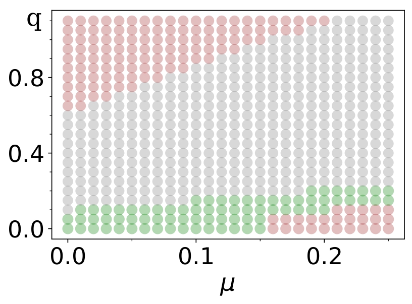
We numerically solve the self consistent equations for order parameters to get the corresponding values and use them to compute the current as given in Eq. 18. Before presenting our results for the beam-splitter current we briefly discuss the phase diagram in q vs $\mu$ plane where q is the nesting vector and $\mu$ denotes the amount of doping in the hole or electron pocket. In Fig. 3 we present the phase diagram obtained after numerically solving the self-consistent equations as described in Sec.II. The main feature of the phase diagram is that the co-existence phase which is the salient aspect of Iron-pnictide superconducting system exists for specific values of q and $\mu$. For example, to get the co-existence phase a finite nesting(finite values of q) is needed as evident from Fig. 3 . Also for very large values of q, the coexistence phase ceases to exist yielding only superconducting phase. Here we briefly compare our numerical phase diagram to that obtained in reference chubukov2. For zero nesting case, i.e. q=0 we observe a transition from pure SDW to pure SC phase around 0.15 doping or the mismatch factor between the hole and electron pocket as previously obtained at zero temperaturechubukov2. It is important to note that $\mu$ is same as the $\delta_{0}$ considered there. Also for q$\neq 0$ case, the transition happens at larger values of $\mu$ than which is obtained at q$=0$. Later we present further comparison of density of state calculation with the previous results in Sec. IV.3 which has been used to benchmark our result. In our numerical analysis, we have taken $V_{s}=2.5$ and $V_{m}=3.0$ and chemical potential is initially kept at 1.7 which determines the initial pocket sizes(i.e. before doping) to standardise our results with the previous workchubukov2. Value of chemical potential is taken in the units of meV. It may be noted that in Eq. 2 $\bm{k}^{2}$ is to be understood as $\hbar^{2}\bm{k}^{2}$. We know that using value of $|\bm{k}|\sim 2\pi/a$ where $a$ is of the order of Angstrom, one finds $\frac{\hbar^{2}\bm{k}^{2}}{2m}$ of the order of meV. In our numerical calculation we have taken $m_{c}=m_{f}=1$ in Eq. 2(instead of 0.51 meV) which implies that the lattice spacing $a$ to be appropriately scaled to a higher value $a\rightarrow\sqrt{2.0}$ Angstrom (approximately) which is more realistic. The value of $\bf q$ is to be understood of the order of $2\pi/a$. Value of $\Delta$ is to be understood in meV as well. As we have plotted $\mathcal{I}_{D}$ instead of $\mathcal{I}_{1}$, the unit of $\mathcal{I}_{D}$ is $\rm{meV}^{-2}$ where as the unit of q is $\rm{Angstrom}^{-1}$. Further we have confirmed the previous finding that the sign change of the superconducting gaps between the hole and electron pocket i.e $\Delta_{c}=-\Delta_{f}$ happens only when $V_{s}$ is positive. To complete the understanding of phase diagram given in Fig. 3, we have plotted the amplitude of superconducting gap $\Delta$ and magnitude of magnetic order parameter $\bf m$ in q$-\mu$ plane in Fig. 4 (a) and (b) respectively. These clearly shows that only in the coexistence phase both the parameters are finite. We refer reference chubukov2; araujo; bang; hu-ting-zhu; jiang-li-wang for more details on the mechanism of magnetic and superconducting ordering and the phase transitions for the interested reader.

Finally In Fig. 4 (c), we plotted the beam-splitter current in the q$-\mu$ plane for $k_{f}\delta r=0$ which clearly shows that in the superconducting phase at low q regime current is significantly higher than in the coexistence phase. However in the coexistence phase the current is finite though lower in magnitude than that in pure superconducting phase. If we zoom in the current in coexistence phase as given in Fig. 4 (d), we find that the current is higher in some region and lower in some region depending on the values of q and $\mu$. In subsequent discussion we describe in detail how the current behaves as a function of $k_{f}\delta r$ for various fixed values of $\mu$ and q.

Till now we have discussed the scenario where only one of the two electrons(or holes) from the electron (or hole) pocket is collected at either dot and the second electron (or hole) is collected at remaining dot. The current generated from this process is the entangled beam-splitter current which is matter of interest to us. However the alternative process such as tunneling of two electrons (or holes) via same dot is a real possibility which yields a contribution to current itself. There are two processes in which electron participating in the Cooper pair can tunnel via same dot. Case (I): First one electron(or hole) tunnels from the superconductor to dot-A let’s say, and then following it the second electron(or hole) also tunnel to the same dot, as a result there are two electrons (or holes) at the same dot which costs an additional Coulomb repulsion energy of U. Thus this virtual state is suppressed by a factor 1/U. Finally the two electrons(holes) leave the dot and tunnel to the lead. Case (II): In the other process one electron (or hole) tunnels to say dot-A and then subsequently leaves the dot and tunnels further to lead-A, leaving an excitation on superconductor that costs additional energy $\Delta$ before finally the second electron tunnels to the lead-A via dot-A. The current taking into account these two processes can be written as,

$\gamma_{s}=2\pi\nu_{s}|T_{DS}|^{2}$ with $\nu_{s}$ is the density of states of the superconductor. $\gamma=\gamma_{1}+\gamma_{2}$ with $\gamma_{l}=2\pi\nu_{l}|T_{DL}|^{2}$ with $\nu_{l}$ being the density of states at lead ’$l$’. The expression for $\mathcal{A^{\prime}}_{k}$ and $\mathcal{A}^{\prime\prime}_{k}$ are given below.

In the above $\tilde{k}=-k$ and expressions for $E_{i,k},u^{c}_{i,k},u^{f}_{i,k}$ and $u^{c}_{i,\tilde{k}},u^{f}_{i,\tilde{k}}$ are given in the Appendix C. Now in the $\mathcal{I}_{S}$ as given in Eq. 20, there are two contributions for above mentioned processes which would add up. For detailed calculation of current we request the reader to look into the Appendix-A. To have a comparison between the current as given in Eq. 18 and in Eq. 20, we estimate the ratio between the two. It is straightforward to obtain,

Clearly $\mathcal{I}_{D}>2\gamma^{2}{\mathcal{I}_{S}}$ is the the desired regime where $\mathcal{I}_{1}$ dominates $\mathcal{I}_{2}$. As shown in Fig. 8, for $\gamma=0.25$ $\mathcal{I}_{1}$ is larger than $\mathcal{I}_{2}$ for some finite values of $k_{f}\delta r$. We also observe that a decrease of $\gamma$ from $0.25$ to $0.10$ rapidly increases the efficiency of beam-splitter current to larger values of $k_{f}\delta r$.

Before we conclude and summarize our study, it is imperative to compare the beam-splitter arrangement studied in earlier pioneering work by Daniel loss and collaborators daniel and subsequent extension for graphene based superconductor by Firoz Islam et.al firoz. Apart from the inherent entangled nature of beam-splitter current, the salient feature of the beam-splitter current for an ideal s-wave BCS supercurrent is characteristic oscillation of current with $k_{f}\delta r$ which is also present in graphene based superconductor and also in the present study. Whereas the chemical potential determines the overall magnitude of the beam-splitter current. However there is an important difference found on the dependency of magnitude of beam-splitter current on chemical potential for normal BCS superconductor (and graphene based superconductor) with the iron-pnictide superconductor considered here. The beam-splitter current monotonically decreases as the chemical potential is decreased for ordinary BCS superconductor and graphene based superconductor. But for iron-pnictide system the dependence of overall magnitude of current is non-monotonous with the chemical potential. The reason is the quasi-particle contributing to the beamsplitter current originates from a single fermi-pocket in case of BCS superconductor and graphene based superconductor and thus changing chemical potential has monotonous dependency on the current. However for iron-pnictide the contribution to the beam-splitter current comes from quasi-particles originating from hole and electron pockets separeted by a momenta $Q$. The change of chemical potential effects the size of the electron and hole pocket in opposite way, i.e if electron pocket size is decreased, hole pocket size is increased. Due to the interdependency of beam-splitter current on both the pockets non-trivially, the current varies non-monotonously with the change on chemical potential. Apart from this important difference there are some other significant differences between iron-pnictide superconductor and graphene based superconductor. First of all in graphene the mechanism of superconductivity is not yet established and for this reason proximity based superconductor is assumed. The proximity induced supercondctor considered earlier included both s-wave and p-wave superconductor ordering defined as $\Delta_{0}=<\alpha_{i\uparrow}\alpha_{i\downarrow}>=<\beta_{i\uparrow}\beta_{i\downarrow}>$ and $\Delta_{1}\sim<\alpha_{i\uparrow}\beta_{j\downarrow}-\alpha_{i\downarrow}\beta_{j\uparrow}>$. Here $\alpha$ and $\beta$ denote the two sublattices in honeycomb lattice. The problem finally reduces as two copies of BCS Hamiltonian interms of $c$ and $d$ operator which are linear combinations of original $\alpha$ and $\beta$ by $\alpha_{ks}=\frac{1}{\sqrt{2}}(c_{ks}+d_{ks}),\beta_{ks}=\frac{1}{\sqrt{2}}e^{-i\phi_{k}}(c_{ks}-d_{ks})$. The bogoliubov quasi-particle energy in the“$c$” and “$d$” channels are given by $E_{k,\nu}=\sqrt{(\xi_{k}+\nu\mu)^{2}+(g_{0}\Delta+\nu g_{1}\Delta_{1}|\gamma_{k}|)^{2}}$, where $\nu=\pm$, where $\nu=+$ for $c$-channel and $\nu=-$ for $d$-channel. The Bogoliubov quasi-particles in the $c$-channel are given by $c_{k,\uparrow}=u_{k,+}\gamma_{1k\uparrow}+v_{k,+}\gamma^{\dagger}_{1-k\downarrow},c_{-k,\downarrow}=u_{k,+}\gamma_{1-k\downarrow}-v_{k,+}\gamma^{\dagger}_{1k\uparrow}$. The equivalent relations for the $d$-channels are given by $d_{k,\uparrow}=u_{k,-}\gamma_{2k\uparrow}+v_{k,-}\gamma^{\dagger}_{2-k\downarrow},d_{-k,\downarrow}=u_{k,+}\gamma_{2-k\downarrow}-v_{k-}\gamma^{\dagger}_{2k\uparrow}$. Here $u_{k,\nu}=\frac{1}{\sqrt{2}}(1+\frac{\xi_{k}}{E_{k,\nu}})^{1/2}$ and $v_{k,\nu}=\frac{1}{\sqrt{2}}(1-\frac{\xi_{k}}{E_{k,\nu}})^{1/2}$. It has been reported that when only $\Delta_{0}$ is present the beam-splitter current is larger than the case where $\Delta_{0}$ and $\Delta_{1}$ are both present. Though for both the cases the physical problem remains two separeted copies of BCS Hamiltonian, the total superconducting quasi-particle density changes when the combinations of order parameters are different. This is evident as the superconducting number density depends on $\sum_{k,\nu}u_{k\nu}v_{k\nu}$ and $u_{k\nu}$ and $v_{k\nu}$ which depends on $E_{k,\nu}$ through $\Delta_{0}$ and $\Delta_{1}$ differently. Thus the physics relies on the re-distribution of quasi-particle density in each blocks. The relation between $c$ and $d$ fermion on the Bogoliubov quasiparticles can be readily compared with the Eqn 52 to Eqn 55. It is evident that in the present case the Bogolubov quasi-particles in $c$ and $f$ channels are not decoupled due to the presence of magnetic order parameters. In the graphene based superconductor such couplings are absent. This coupling between the hole and electron pocket which gives rise to magnetic order parameters are the crucial ingredients for the iron-pnictide based beam-splitter studied here. This gives rise to the non-trivial interference pattern between the two bogoliubov quasiparticles coming from hole and electron pockets.

To summarize we have proposed a Cooper pair beam splitter arrangement for Iron-pnictide superconductor which is known for hosting Cooper pairs responsible for superconducting property as well as inherent magnetic ordering. The co-existence of these two seemingly non-inclusive order parameters in a given material provides an interesting platform to investigate the consequences in a Cooper pair beam splitter current. We have considered various realistic situations found in actual materials such as zero nesting and finite nesting chubukov1, equal and unequal size of hole and electron pockets etc. Most notably our finding indicates that in general the beam splitter current depends non-monotonically on electron $\mu_{c}$ and hole doping $\mu_{f}$ as well as on the magnitude of nesting vector $|{\bf q}|$. In all these cases there are a critical values for which the current is maximum. We believe that this fact might be useful in practical application such as switching and quantum gate applications. In the absence of magnetic ordering the beam splitter current is additive due to hole and electron pocket. However in the co-existence phase due to the entanglement between fermions in electron and hole pocket there are quantum interference effect which results in characteristic oscillations of beam splitter current with respect to nesting vector.
It may also be noted that though in the beamsplitter set up we have assumed $|T_{DS}|<|T_{DL}|$ we do not expect any Kondo effect to set in within the quantum dots because initially in the static limit the quantum dots are taken as vacuum state. Also the tunneling of electron from the lead to quantum dots are surpressed by the grand canonical distribution function $\infty~\rm{exp}(-\Delta\mu/K_{B}T)$ where $\Delta\mu$ is the bias voltage. Even a negligible amount of tunneling of normal electron from lead to quantum dot are going to be in even numbers due to participation of electrons of either spins. This would also make the total number of electrons on quantum dots to be even number which works against Kondo effect to be realized.
The effect of external pressure may be an useful way to control the nesting vectors as found before Vladimir. It may be noted that we have done our calculation of beam splitter current at zero temperature for a prototype iron-pnictide superconductor whereas in real material such superconductivity having coexistence of magnetic order and superconducting order happens upto quite large temperature in comparison to conventional BCS superconductor. We leave the question of finite temperature effect of this beam splitter set up for a future study. However given the fact that all the existing studies so far on beam splitter current is at zero temperature BCS like superconductor and the finite temperature stability of Iron-pnictide superconductor for a wide range of temperature, we think that the study done here would be a realizable at higher temperature than a conventional BCS supercondctor based beam-splitter set up.

However we note that the magnitude of the Iron-pnictide based beam-splitter current is smaller in the co-existence phase in order of magnitude than the conventional two dimensional BCS superconductor based beam-splitter current. With the recently proposed protocol of measuring current produced by single electron detection bylander; fujisawa one can expect that the current may be measured. However one also needs to consider the signal to noise ratio for such measurement. We think that our present study would motivate for further investigations on other aspects such as effect of ferromagnetic proximity effect hofstetter1; burset-2011, effect of impurity hofstetter1; burset-2011 and Bells inequalitysamuelsson-2003.

Finally we note that with the recent significant developments in the field of theoretical and experimental topological insulator based superconductor named topological superconductor, the beam splitter arrangement could serve as an unique set up to detect various quantum mechanical aspect of the topological states as well as the superconducting properties. Recently superconductivity at room temperature has been observed in few-layer Stanene which also host a quantum spin hall phasemenghan-liao. How the robustness of the topological states and superconducting state responds due to various perturbations and disorder is an interesting aspect that can be looked at these topological superconductors menghan-liao; shu-ping-lee; sean-hart; zhao. Further we think the presence of inter-valley scattering in Chern insulator based moire superconductor or in twisted bilayer may have characteristic oscillations or interference pattern in the beam-splitter set up arrangement considered here chuan-wu; ashvin; efetov; ipsita. However the scope of this study remains open in future.

References

- (1) J. J. Sakurai, Jim Napolitano, Modern Quantum Mechanics, Cambridge University Press, 3rd Edition(2020)
- (2) Michael A. Neilson and Isacc L. Chuang Quantum Computations and Quantum Informations, Cambridge University Press (2003).
- (3) David P. DiVincenzo, Fortschr. Phys. 48, (2000) 9-11, 771-783
- (4) Ivan Djordjevic, Quantum Information Processing and Quantum Error Correction, 2012
- (5) T. Bækkegaard, L. B. Kristensen, N. J. S. Loft, C. K. Andersen, D. Petrosyan & N. T. Zinner, Scientific Reports volume 9, Article number: 13389 (2019)
- (6) Ashley Montanaro, npj Quantum Information volume 2, Article number: 15023 (2016)
- (7) Walter Pötz Ulrich Hohenester Jaroslav Fabian, Quantum Coherence From Quarks to Solids, Springer
- (8) T. van der Sar, Z. H. Wang, M. S. Blok, H. Bernien, T. H. Taminiau, D. M. Toyli, D. A. Lidar, D. D. Awschalom, R. Hanson & V. V. Dobrovitski, Nature volume 484, pages82–86(2012)
- (9) Tinkham, Michael (1996). Introduction to Superconductivity. Dover Publications.
- (10) Yi Zhou, Kazushi Kanoda, and Tai-Kai Ng, Rev. Mod. Phys. 89, 025003 (2017)
- (11) Lucile Savary and Leon Balents, 2017 Rep. Prog. Phys. 80, 016502
- (12) G Baskaran, Z Zou and P W Anderson, Sol. State Commun. 63, 973 (1987)
- (13) A. Einstein, B. Podolsky, and N. Rosen, Phys. Rev. 47, 777 (1935)
- (14) J.S. Bell, Speakable and unspeakable in quantum mechanics, Cambridge University Press, Cambridge, 1987
- (15) A. Peres, Quantum theory: Concepts and methods, Kluwer, Dordrecht, 1993.
- (16) Bei Zeng, Xie Chen, Duan-Lu Zhou, Xiao-Gang Wen, Quantum Information Meets Quantum Matter – From Quantum Entanglement to Topological Phase in Many-Body Systems, Springer, 2019(Book). arXiv:1508.02595
- (17) Nicolas Laflorencie, Physics Report Volume 643, 1-59(2016)
- (18) Andreas Osterloh, arXiv:0810.1240
- (19) Patrik Recher, Eugene V. Sukhorukov, and Daniel Loss, Phys. Rev. B. 63, 165314 (2001)
- (20) L.Hofstetter, S.Csonka, J.Nygard and C.Schönenberger, Nature, Vol 461, 08432, 2009
- (21) L. G. Herrmann, F. Portier, P. Roche, A. L. Yeyati, T. Kontos, and C. Strunk, Phys. Rev. Lett. 104, 026801 (2010).
- (22) P.Burset,W.J.Herrera,and A.Levy Yeyati, Phys. Rev. B 84, 115448 (2011)
- (23) Koji Sato,and Yaroslav Tserkovnyak, Phys. Rev. B 90, 045419, 2014
- (24) Mattia Mantovani, Wolfgang Belzig, Gianluca Rastelli, and Robert Hussein, Phys. Rev. Research 1, 033098 (2019)
- (25) Constantinos Valagiannopoulos, Phys. Rev. Applied 12, 054042 (2019)
- (26) SK Firoz Islam and Arijit Saha,Phys. Rev. B. 96, 125406 (2017)
- (27) Michael R. Norman,The Challenge of Unconventional Superconductivity, 8 APRIL 2011 VOL 332 SCIENCE
- (28) Yunkyu Bang and G R Stewart 2017 J. Phys.: Condens. Matter 29 123003
- (29) I. I. Mazin, D. J. Singh, M. D. Johannes, and M. H. Du, Phys. Rev. Lett. 101, 057003 (2008)
- (30) M.K. Wu et al. Phys. Rev. Lett., 58 (9) (1987), p. 908
- (31) Hideo Hosono, Akiyasu Yamamoto, Hidenori Hiramatsu, Yanwei Ma, Materials Today, Volume 21, Number 3, April 2018
- (32) Hai-Hu Wen and Shiliang Li, Annu. Rev. Condens. Matter Phys. 2011. 2:121–40
- (33) G. R. Stewart, REVIEWS OF MODERN PHYSICS, VOLUME 83, OCTOBER–DECEMBER 2011
- (34) Qimiao Si, Rong Yu, Elihu Abrahams, Nature Rev. Mater. 1, 16017 (2016). arXiv:1604.03566
- (35) F. Steglich, Physica C: Superconductivity and its Applications, Volumes 460–462, Part 1, 2007, Pages 7-12
- (36) D.J.Singh, Acta Physica Polonica A, 121, 2012
- (37) A. Subedi, L. Zhang, D. J. Singh, and M. H. Du, Phys. Rev. B 78, 134514 (2008)
- (38) A. V. Chubukov,Physica C 469, 640, 2009
- (39) A. V. Chubukov,V. Efremov and I. Eremin, Phys. Rev. B 78, 134512 (2008)
- (40) A. B. Vorontsov,M. G. Vavilov and A. V. Chubukov, Phys. Rev. B 81, 174538 (2010)
- (41) M A N Araujo, M Cardoso and P D Sacramento, New Journal of Physics 11 (2009) 113008
- (42) Yunkyu Bang and Han-Yong Choi, Phys. Rev. B 78, 134523 (2008)
- (43) Xiang Hu, C. S. Ting, Jian-Xin Zhu, Phys. Rev. B 80, 014523 (2009)
- (44) Hong-Min Jiang, Jian-Xin Li and Z. D. Wang, Phys. Rev. B 80, 134505(2009)
- (45) M. Sumetskiǐ, Phys. Rev. B 48, 4586 (1993)
- (46) E. Merzbacher, Quantum Mechanics, 3rd ed. (Wiley, New York, 1998), Chap. 20
- (47) Vladimir Cvetkovic and Zlatko Tesanovic, Phys. Rev. B 80, 024512 (2009)
- (48) L. Hofstetter, A. Geresdi, M. Aagesen, J. Nygard, C. Schönenberger, and S. Csonka, Phys. Rev. Lett 104, 246804(2010)
- (49) J.Rech, D.Chevallier, T.Jonckheere, and T. Martin, Phys. Rev B 85, 035419 (2012)
- (50) P. Samuelsson, E. V. Sukhorukov, and M. Büttiker, Phys. Rev. Lett. 91, 157002 (2003)
- (51) Jonas Bylander, Tim Duty and Per Delsing, Nature volume 434, pages 361–364(2005)
- (52) Toshimasa Fujisawa, Toshiaki Hayashi, Ritsuya Tomita, Yoshiro Hirayama, Science 312, pages 1634 (2006)
- (53) Menghan Liao, Yunyi Zang, Zhaoyong Guan, Haiwei Li, Yan Gong, Kejing Zhu, Xiao-Peng Hu, Ding Zhang, Yong Xu, Ya-Yu Wang, Ke He, Xu-Cun Ma, Shou-Cheng Zhang and Qi-Kun Xue, Nature Phys 14, 344–348 (2018). https://doi.org/10.1038/s41567-017-0031-6
- (54) Shu-Ping Lee, Karen Michaeli, Jason Alicea, and Amir Yacoby, Phys. Rev. Lett 113, 197001 (2014)
- (55) Sean Hart, Hechen Ren, TimoWagner, Philipp Leubner, Mathias Mühlbauer, Christoph Brüne, Hartmut Buhmann, Laurens W. Molenkamp and Amir Yacoby, Nature Phys 10, 638–643 (2014). https://doi.org/10.1038/nphys3036
- (56) Chenxiao Zhao, Leiqiang Li, Liying Zhang , Jin Qin, Hongyuan Chen, Bing Xia, Bo Yang, Hao Zheng, Shiyong Wang, Canhua Liu, Yaoyi Li, Dandan Guan, Ping Cui, Zhenyu Zhang,and Jinfeng Jia, Phys. Rev. Lett 128, 206802(2022)
- (57) Xiao-Chuan Wu, Yichen Xu, Chao-Ming Jian, and Cenke Xu, Phys. Rev. B 100, 155138 (2019).
- (58) Yi-Zhuang You and Ashvin Vishwanath, npj Quantum Materials 4, 16 (2019)
- (59) Petr Stepanov, Ming Xie, Takashi Taniguchi, Kenji Watanabe, Xiaobo Lu, Allan H. MacDonald, B. Andrei Bernevig, and Dmitri K. Efetov, Phys. Rev. Lett. 127, 197701, (2021).
- (60) Ipsita Das, Xiaobo Lu, Jonah Herzog-Arbeitman, Zhi-Da Song, Kenji Watanabe, Takashi Taniguchi, B. Andrei Bernevig and Dmitri K. Efetov, Nature Physics 17, 710–714 (2021).