C-MinHash:
Practically Reducing Two Permutations to Just One

Xiaoyun Li Ping Li Affiliation: Cognitive Computing Lab Affiliation: Baidu Research Affiliation: 10900 NE 8th St. Bellevue, WA 98004, USA Email: {xiaoyunli, liping11}@baidu.com

Abstract

Traditional minwise hashing (MinHash) requires applying $K$ independent permutations to estimate the Jaccard similarity in massive binary (0/1) data, where $K$ can be (e.g.,) 1024 or even larger, depending on applications. The recent work on C-MinHash (Li and Li 2021) has shown, with rigorous proofs, that only two permutations are needed. An initial permutation is applied to break whatever structures which might exist in the data, and a second permutation is re-used $K$ times to produce $K$ hashes, via a circulant shifting fashion. Li and Li 2021 has proved that, perhaps surprisingly, even though the $K$ hashes are correlated, the estimation variance is strictly smaller than the variance of the traditional MinHash.

It has been demonstrated in Li and Li 2021 that the initial permutation in C-MinHash is indeed necessary. For the ease of theoretical analysis, they have used two independent permutations. In this paper, we show that one can actually simply use one permutation. That is, one single permutation is used for both the initial pre-processing step to break the structures in the data and the circulant hashing step to generate $K$ hashes. Although the theoretical analysis becomes very complicated, we are able to explicitly write down the expression for the expectation of the estimator. The new estimator is no longer unbiased but the bias is extremely small and has essentially no impact on the estimation accuracy (mean square errors). An extensive set of experiments are provided to verify our claim for using just one permutation.

1 Background

Given two binary data vectors $\bm{v},\bm{w}\in\{0,1\}^{D}$ in $D$ dimensions, the Jaccard (resemblance) similarity $J(\bm{v},\bm{w})$ is defined as

\displaystyle J(\bm{v},\bm{w})\triangleq\frac{a}{f},\hskip 14.45377pt\text{ where }\ a\triangleq\sum_{i=1}^{D}\mathbbm{1}\{v_{i}=w_{i}=1\},\hskip 14.45377ptf\triangleq\sum_{i=1}^{D}\mathbbm{1}\{v_{i}=1\ \text{or}\ w_{i}=1\}.

(1)

Of course, practical applications may need to deal with billions or thousands of billions of data vectors, not just two vectors. How to effectively store/transmit/retrieve the data and how to efficiently compute or estimate similarities among data vectors has always been a long-lasting research and engineering challenge.

Minwise hashing (MinHash) (Broder 1997; Broder et al. 1997; Broder et al. 1998; Li and Church 2005; Li and König 2011) is a standard technique for efficiently estimating the Jaccard similarity in massive binary data. Classical MinHash requires applying $K$ (independent) random permutations on each data vector to produce $K$ hash values. The recent work by Li and Li 2021 proposed using just two random permutations: an initial permutation breaks whatever structures in the data vector and a second permutation is re-used $K$ times to generate $K$ hashes. They proved their surprising (and rather involved) theoretical finding that the estimation variance in their scheme is actually strictly smaller than the variance of the original MinHash.

Li and Li 2021 named their method as C-MinHash- $(\sigma,\pi)$ , where $\sigma$ stands for the initial permutation and $\pi$ for the second permutation. A natural and immediate question to ask is why we really need two permutations. Indeed, Li and Li 2021 also analyzed and experimented with C-MinHash- $(0,\pi)$ , where “0” means that the initial permutation was not used. They reported that the performance of C-MinHash- $(0,\pi)$ was not satisfactory, because natural datasets typically do exhibit various structures.

In this paper, we propose C-MinHash- $(\pi,\pi)$ . That is, we just use one permutation $\pi$ for both the “initial” permutation to break the existing structures in the data and the “second” permutation to generate $K$ hashes. In Li and Li 2021, they used two independent permutation mainly for simplifying the theoretical analysis, otherwise the complicated dependency would make the analysis challenging. In this work, we are able to write down explicitly the sophisticated expression for the expectation (mean) of the estimator for C-MinHash- $(\pi,\pi)$ . Although the estimator is no longer strictly unbiased, the bias is so small that it can be safely neglected. We verify this claim via an extensive set of experiments.

2 Review of MinHash and C-MinHash

Input: Binary data vector $\bm{v}\in\{0,1\}^{D}$ , $K$ independent permutations $\pi_{1},...,\pi_{K}$ : $[D]\rightarrow[D]$ .

Output: $K$ hash values $h_{1}(\bm{v}),...,h_{K}(\bm{v})$ .

For $k=1$ to $K$

$h_{k}(\bm{v})\leftarrow\min_{i:v_{i}\neq 0}\pi_{k}(i)$

End For

Algorithm 1 Minwise-hashing (MinHash)

Algorithm 1 describes the procedure for the classical MinHash, using the example of one vector $\bm{v}\in\{0,1\}^{D}$ . Note that the same set of permutations would be needed for all data vectors. After having generated $K$ hashes for both $\bm{v},\bm{w}\in\{0,1\}^{D}$ , i.e., $h_{k}(\bm{v})$ , $h_{k}(\bm{w})$ , $k=1,2,...,K$ , the estimator of $J(\bm{v},\bm{w})$ , i.e., the Jaccard similarity between $\bm{v}$ and $\bm{w}$ , is simply

		$\displaystyle\hat{J}_{MH}(\bm{v},\bm{w})=\frac{1}{K}\sum_{k=1}^{K}\mathbbm{1}\{h_{k}(\bm{v})=h_{k}(\bm{w})\},$		(2)
		$\displaystyle\mathbb{E}[\hat{J}_{MH}]=J,\hskip 28.90755ptVar[\hat{J}_{MH}]=\frac{J(1-J)}{K}.$		(3)

Input: Binary data vector $\bm{v}\in\{0,1\}^{D}$ , Permutation vectors $\pi$ and $\sigma$ : $[D]\rightarrow[D]$

Output: Hash values $h_{1}(\bm{v}),...,h_{K}(\bm{v})$

Initial permutation: $\bm{v}^{\prime}$ = $\sigma(\bm{v})$

For $k=1$ to $K$

Shift $\pi$ circulantly rightwards by $k$ units: $\pi_{k}=\pi_{\rightarrow k}$

$h_{k}(\bm{v})\leftarrow\min_{i:v_{i}^{\prime}\neq 0}\pi_{\rightarrow k}(i)$

End For

Algorithm 2 C-MinHash-

(\sigma,\pi)

Refer to caption — Figure 1: An illustrative example of C-MinHash- $(\sigma,\pi)$ using two independent permutations: $\sigma$ for initial permutation and $\pi$ for generating $K$ hashes. The original data vector has two non-zeros, $v_{1}=v_{2}=1$ . In this example, $h_{1}(\bm{v})=1$ , $h_{2}(\bm{v})=3$ .

Algorithm 2 presents the procedure for C-MinHash- $(\sigma,\pi)$ developed in Li and Li 2021, where the initial permutation $\sigma$ is first applied to break the structures in the data and the second permutation $\pi$ is re-used $K$ times to produce $K$ hashes in a circulant shifting fashion. Figure 1 illustrates the procedure using a concrete example. The unbiased estimator of C-MinHash- $(\sigma,\pi)$ is then

\displaystyle\hat{J}_{\sigma,\pi}(\bm{v},\bm{w})=\frac{1}{K}\sum_{k=1}^{K}\mathbbm{1}\{h_{k}(\bm{v})=h_{k}(\bm{w})\},

(4)

where $h_{k}$ ’s are the hash values generated by Algorithm 2. An interesting theoretical result was proved in Li and Li 2021 on the uniform superiority of C-MinHash- $(\sigma,\pi)$ over the original MinHash in terms of the Jaccard estimation variance.

Theorem 2.1.

(Li and Li 2021) It holds that $Var[\hat{J}_{\sigma,\pi}(\bm{v},\bm{w})]<Var[\hat{J}_{MH}(\bm{v},\bm{w})]$ , $\forall\bm{v},\bm{w}\in\{0,1\}^{D}$ , $K\leq D$ , and $J\in(0,1)$ .

The above result is surprising because it gives an example of less work leads to better performance. It was also shown in Li and Li 2021 that the initial permutation $\sigma$ is necessary otherwise the estimation accuracy typically would drop due to the existing structures in the original data. This theoretical result can be beneficial in the design of hashing methods. For example, to ensure the estimation accuracy strictly follows the theory, a naive implementation of the original MinHash would be simply to store $K$ permutations: $[D]\rightarrow[D]$ . When $D=2^{30}$ (which might be sufficient for many applications), it is unrealistic to store $K$ such permutations if $K=1024$ . On the other hand, it is probably trivial to store just two such permutations.

3 C-MinHash- $(\pi,\pi)$ : Reducing Two Permutations to Just One

In this paper, we propose C-MinHash- $(\pi,\pi)$ , by using just one permutation $\pi$ for both initially shuffling the data and generating $K$ hashes via circulant shifting. Algorithm 3 is almost the same as Algorithm 2.

Input: Binary data vector $\bm{v}\in\{0,1\}^{D}$ , A permutation vector $\pi$ : $[D]\rightarrow[D]$

Output: Hash values $h_{1}(\bm{v}),...,h_{K}(\bm{v})$

Initial permutation: $\bm{v}^{\prime}$ = $\pi(\bm{v})$

For $k=1$ to $K$

Shift $\pi$ circulantly rightwards by $k$ units: $\pi_{k}=\pi_{\rightarrow k}$

$h_{k}(\bm{v})\leftarrow\min_{i:v_{i}^{\prime}\neq 0}\pi_{\rightarrow k}(i)$

End For

Algorithm 3 C-MinHash-

(\pi,\pi)

Analogously, we have the Jaccard estimator for C-MinHash- $(\pi,\pi)$ :

\displaystyle\hat{J}_{\pi,\pi}=\frac{1}{K}\sum_{k=1}^{K}\mathbbm{1}\{h_{k}(\bm{v})=h_{k}(\bm{w})\},

(5)

with $h_{k}$ ’s are the hash values output by Algorithm 3. Strictly speaking, $\hat{J}_{\pi,\pi}$ is no longer unbiased, but we will show that the bias has essentially no impact on the estimation accuracy in terms of the mean square error: MSE = bias² + variance. While the theoretical analysis for C-MinHash- $(\sigma,\pi)$ in Li and Li 2021 was already rather involved, analyzing C-MinHash- $(\pi,\pi)$ becomes much more difficult. Nevertheless, we are able to at least derive the explicit expression for the expectation (mean) of the estimator:

\displaystyle\mathbb{E}[\hat{J}_{\pi,\pi}]=\frac{1}{K}\sum_{k=1}^{K}\mathbb{E}[\mathbbm{1}\{h_{k}(\bm{v})=h_{k}(\bm{w})\}].

(6)

Definition 3.1.

For two binary data vectors $\bm{v},\bm{w}\in\{0,1\}^{D}$ , define the location vector as $\bm{x}\in\{O,\times,-\}^{D}$ , with $\bm{x}_{i}$ being “ $O$ ”,“ $\times$ ”,“ $-$ ” when $\bm{v}_{i}=\bm{w}_{i}=1$ , $\bm{v}_{i}+\bm{w}_{i}=1$ and $\bm{v}_{i}=\bm{w}_{i}=0$ , respectively.

The collision of hash samples can be concretely described by the location vector $\bm{x}$ after permutation. If the first “ $O$ ” appears before the first “ $\times$ ” (counting from small to large), then the hash sample collides. We will use hyper( $N,m,n_{1},...,n_{p}$ ) to denote the $p$ -dimensional hyper-geometric distribution, where $N$ is the total number of instances, $m$ is number of draws and $n_{i}$ , $i=1,...,p$ is the size of each class.

Theorem 3.1.

Assume $K\leq D$ and let $a,f$ be defined as (1). The location vector $\bm{x}$ is defined in Definition 3.1. Denote $\mathcal{B}_{1}=\{i:\bm{x}_{i}=O\}$ , $\mathcal{B}_{2}=\{i:\bm{x}_{i}=\times\}$ and $\mathcal{B}_{3}=\{i:\bm{x}_{i}=-\}$ . For $a\leq j\leq D$ and $1\leq k\leq K$ , define

\displaystyle\mathcal{A}_{-}(j)=\{\bm{x}_{i}:(i+k-1\ mod\ D)+1\leq j\},\quad\mathcal{A}_{+}(j)=\{\bm{x}_{i}:(i+k-1\ mod\ D)+1>j\}.

Let $n_{-,1}(j)=|\{\bm{x}_{i}=O:i\in\mathcal{A}_{-}(j)\}|$ be the number of “ $O$ ” points in $\mathcal{A}_{-}(j)$ . Analogously let $n_{-,2}(j),n_{-,3}(j)$ be the number of “ $\times$ ” and “ $-$ ” points in $\mathcal{A}_{-}(j)$ , and $n_{+,1}(j),n_{+,2}(j),n_{+,3}(j)$ be the number of “ $O$ ”, “ $\times$ ” and “ $-$ ” points in $\mathcal{A}_{+}(j)$ . Then, for the $k$ -th C-MinHash- $(\pi,\pi)$ hash collision indicator,

\displaystyle\mathbb{E}[\mathbbm{1}\{h_{k}(\bm{v})=h_{k}(\bm{w})\}]=\sum_{j=1}^{D}\sum_{Z\in\Theta_{j}}P_{j}(Z)\cdot\Big\{\sum_{i=1}^{3}\Psi_{i}(j)+\sum_{i\in\mathcal{B}_{1}}(1-\frac{z_{-,1}}{n_{-,1}(i^{*})})\tilde{P}_{1}\Big\},

where $P_{j}(Z)$ is the density function of $Z=(z_{-,k}|_{1}^{3},z_{+,k}|_{1}^{3})$ which follows hyper( $D,D-f,n_{-,k}(j)|_{1}^{3},n_{+,k}(j)|_{1}^{3}$ ), with domain $\Theta_{j}$ . For $q=1,2,3$ , denote $\mathbbm{1}^{\#}_{q}=\mathbbm{1}\{j^{\#}\in\mathcal{B}_{q}\}$ , and

		$\displaystyle\Psi_{q}(j)=\sum_{i\in\mathcal{B}_{q},j<i^{*}}\sum_{p=1}^{3}\mathbbm{1}^{\#}_{p}\big(1-\frac{z_{-,p}}{n_{-,p}(j)}+\mathbbm{1}\{q=3\}(2\frac{z_{-,p}}{n_{-,p}(j)}-1)\big)(1-\frac{z_{+,q}}{n_{+,q}(j)})\tilde{P}_{q}\bar{J}_{q}$
		$\displaystyle\hskip 21.68121pt+\sum_{i\in\mathcal{B}_{q},j>i^{}}\Big[\mathbbm{1}^{\#}_{q}(1-\frac{z_{-,q}}{n_{-,q}(j)})(1-\frac{z_{-,q}}{n_{-,q}(j)-1})+\sum_{p\neq q}^{3}\mathbbm{1}^{\#}_{p}(1-\frac{z_{-,q}}{n_{-,q}(j)})(1-\frac{z_{-,p}}{n_{-,p}(j)})\Big]\tilde{P}_{q}J^{},$

where $i^{*}=(i+k-1\ mod\ D)+1$ , $i^{\#}=(i-k-1\ mod\ D)+1$ , $\forall i$ . Define $J^{*}=\frac{a-r_{1}}{f-r_{1}-r_{2}}$ , and

		$\displaystyle\tilde{P}_{1}=\tilde{P}_{2}=\frac{1}{r_{1}+r_{2}}\frac{\binom{b_{0}}{r_{3}}\binom{D-j-b_{0}}{r_{1}+r_{2}-1}}{\binom{D-f}{r_{3}}\binom{f}{r_{1}+r_{2}}},\hskip 7.22743pt\tilde{P}_{3}=\frac{1}{r_{3}}\frac{\binom{b_{0}}{r_{3}-1}\binom{D-j-b_{0}}{r_{1}+r_{2}}}{\binom{D-f}{r_{3}}\binom{f}{r_{1}+r_{2}}},$
		$\displaystyle\bar{J}_{q}=\frac{r_{1}-\mathbbm{1}\{q=1\}}{D-j-b_{0}}+(1-\frac{r_{1}+r_{2}-\mathbbm{1}\{q\neq 3\}}{D-j-b_{0}})J^{*},\ q=1,2,3,$

where $b_{0}=\sum_{k=1}^{3}z_{+,k}$ , $r_{1}=a-z_{-,1}-z_{+,1}$ , $r_{2}=f-a-z_{-,2}-z_{+,2}$ and $r_{3}=D-f-z_{-,3}-z_{+,3}$ .

Theorem 3.1 says that $\mathbb{E}[\mathbbm{1}\{h_{k}(\bm{v})=h_{k}(\bm{w})\}]$ would be different for different $k$ . For each $k$ , the absolute value of the bias is typically very small, and furthermore, this bias would be averaged out with $K$ hash samples (as illustrated in Figure 2 and Figure 3). Also, from the proof (see Appendix A) we can know that when $a$ and $f$ are fixed, as $D$ increases, $\mathbb{E}[\hat{J}_{\pi,\pi}]$ would converge to $J$ .

Figure 2 presents numerical examples to validate the theory and demonstrate the magnitude of bias² (recall MSE = bias² + variance). We simulate data pairs with a series of $(D,f,a)$ values, where the dimension is fixed as $D=64$ and we vary $f$ and $a$ (recall $a\triangleq\sum_{i=1}^{D}\mathbbm{1}\{v_{i}=w_{i}=1\},\ f\triangleq\sum_{i=1}^{D}\mathbbm{1}\{v_{i}=1\ \text{or}\ w_{i}=1\}$ .) The non-zero entries are randomly assigned. The simulations match perfectly Theorem 3.1. As we can see, bias² is very small ( $10^{-5}$ or even smaller) and approaches 0 as $K$ increases (i.e., the averaging effect).

Furthermore, Figure 3 plots $\mathbb{E}[\mathbbm{1}\{h_{k}(\bm{v})=h_{k}(\bm{w})\}]$ for every $k$ , $1\leq k\leq K$ . Again, the simulation results perfectly match the theory in Theorem 3.1. As $\mathbb{E}[\mathbbm{1}\{h_{k}(\bm{v})=h_{k}(\bm{w})\}]$ can be positive or negative, the overall bias $\mathbb{E}[\hat{J}_{\pi,\pi}]=\frac{1}{K}\sum_{k=1}^{K}\mathbb{E}[\mathbbm{1}\{h_{k}(\bm{v})=h_{k}(\bm{w})\}]$ would approach 0 as $K$ increases, as verified in Figure 2.

Figure 4 plots the MSE = bias²+variance, for comparing the empirical MSEs of C-MinHash- $(\pi,\pi)$ with the theoretical variances of C-MinHash- $(\sigma,\pi)$ in Li and Li 2021. Besides the cases in Figure 2, the bottom two rows of Figure 4 provide more examples where the data vector pairs have a special locational structure. In all figures, the overlapping MSE curves essentially verify our claim that we just need one permutation $\pi$ .

4 Further Empirical Verification

In this section, we present extensive experiments on real data, to further validate that C-MinHash- $(\pi,\pi)$ and C-MinHash- $(\sigma,\pi)$ perform equivalently in Jaccard estimation. We first use 120 pairs of word vectors from the “Words” dataset (Li and Church 2005) to once again validate that the MSE of C-MinHash- $(\pi,\pi)$ basically matches the theoretical variance of C-MinHash- $(\sigma,\pi)$ (which is strictly unbiased).

4.1 MSE Comparisons on Words Dataset

The “Words” dataset (Li and Church 2005) (which is publicly available) contains a large number of word vectors, with the $i$ -th entry indicating whether this word appears in the $i$ -th document, for a total of $D=2^{16}$ documents. The key statistics of the 120 selected word pairs are presented in Table 1. Those 120 pairs of words are more or less randomly selected except that we make sure they cover a wide spectrum of data distributions. Denote $d$ as the number of non-zero entries in the vector. Table 1 reports the density $\tilde{d}=d/D$ for each word vector, ranging from 0.0006 to 0.6. The Jaccard similarity $J$ ranges from 0.002 to 0.95.

In Figures 5 - 12, we plot the empirical MSE along with the empirical bias² for $\hat{J}_{\pi,\pi}$ , as well as the empirical MSE for $\hat{J}_{\sigma,\pi}$ . Note that for $D$ this large, it is numerically difficult to evaluate the theoretical variance formulas in Li and Li 2021. From the results in the Figures, we can observe

•

For all the data pairs, the MSE of C-MinHash- $(\pi,\pi)$ estimator overlaps with the empirical MSE of C-MinHash- $(\sigma,\pi)$ estimator for all $K$ from 1 up to 4096.
•

The bias² is several orders of magnitudes smaller than the MSE, in all data pairs. This verifies that the bias of $\hat{J}_{\pi,\pi}$ is extremely small in practice and can be safely neglected.

We have many more plots on more data pairs. Nevertheless, we believe the current set of experiments on this “Words” dataset should be sufficient to verify that, the proposed C-MinHash- $(\pi,\pi)$ could give indistinguishable Jaccard estimation accuracy in practice compared with C-MinHash- $(\sigma,\pi)$ .

Table 1: 120 selected word pairs from the Words dataset (Li and Church 2005). For each pair, we report the density

\tilde{d}

(number of non-zero entries divided by

D=2^{16}

) for each word as well as the Jaccard similarity

J

	$\tilde{d}_{1}$	$\tilde{d}_{2}$	$J$		$\tilde{d}_{1}$	$\tilde{d}_{2}$	$J$
ABOUT - INTO	0.302	0.125	0.258	NEW - WEB	0.291	0.194	0.224
ABOUT - LIKE	0.302	0.140	0.281	NEWS - LIKE	0.168	0.140	0.172
ACTUAL - DEVELOPED	0.017	0.030	0.071	NO - WELL	0.220	0.120	0.244
ACTUAL - GRABBED	0.017	0.002	0.016	NOT - IT	0.281	0.295	0.437
AFTER - OR	0.103	0.356	0.220	NOTORIOUSLY - LOCK	0.0006	0.006	0.004
AND - PROBLEM	0.554	0.044	0.070	OF - THEN	0.570	0.104	0.168
AS - NAME	0.280	0.144	0.204	OF - WE	0.570	0.226	0.361
AT - CUT	0.374	0.242	0.052	OPPORTUNITY - COUNTRIES	0.029	0.024	0.066
BE - ONE	0.323	0.221	0.403	OUR - THAN	0.244	0.125	0.245
BEST - AND	0.136	0.554	0.228	OVER - BACK	0.148	0.160	0.233
BRAZIL - OH	0.010	0.031	0.019	OVER - TWO	0.148	0.121	0.289
BUT - MANY	0.167	0.116	0.340	PEAK - SHOWS	0.006	0.033	0.026
CALLED - BUSINESSES	0.016	0.018	0.043	PEOPLE - BY	0.121	0.425	0.228
CALORIES - MICROSOFT	0.002	0.045	0.0003	PEOPLE - INFO	0.121	0.138	0.117
CAN - FROM	0.243	0.326	0.444	PICKS - BOOST	0.007	0.005	0.007
CAN - SEARCH	0.243	0.214	0.237	PLANET - REWARD	0.013	0.003	0.018
COMMITTED - PRODUCTIVE	0.013	0.004	0.029	PLEASE - MAKE	0.168	0.141	0.195
CONTEMPORARY - FLASH	0.011	0.021	0.013	PREFER - PUEDE	0.010	0.003	0.0001
CONVENIENTLY - INDUSTRIES	0.003	0.011	0.009	PRIVACY - FOUND	0.126	0.136	0.053
COPYRIGHT - AN	0.218	0.290	0.209	PROSECUTION - MAXIMIZE	0.002	0.003	0.006
CREDIT - CARD	0.046	0.041	0.285	RECENTLY - INT	0.028	0.007	0.014
DE - WEB	0.117	0.194	0.091	REPLY - ACHIEVE	0.013	0.012	0.023
DO - GOOD	0.174	0.102	0.276	RESERVED - BEEN	0.172	0.141	0.108
EARTH - GROUPS	0.021	0.035	0.056	RIGHTS - FIND	0.187	0.144	0.166
EXPRESSED - FRUSTRATED	0.010	0.002	0.024	RIGHTS - RESERVED	0.187	0.172	0.877
FIND - HAS	0.144	0.228	0.214	SCENE - ABOUT	0.012	0.301	0.029
FIND - SITE	0.144	0.275	0.212	SEE - ALSO	0.138	0.166	0.291
FIXED - SPECIFIC	0.011	0.039	0.054	SEIZE - ANYTHING	0.0007	0.037	0.012
FLIGHT - TRANSPORTATION	0.011	0.018	0.040	SHOULDERS - GORGEOUS	0.003	0.004	0.028
FOUND - DE	0.136	0.117	0.039	SICK - FELL	0.008	0.008	0.085
FRANCISCO - SAN	0.025	0.049	0.476	SITE - CELLULAR	0.275	0.006	0.010
GOOD - BACK	0.102	0.160	0.220	SOLD - LIVE	0.018	0.064	0.055
GROUPS - ORDERED	0.035	0.011	0.034	SOLO - CLAIMS	0.010	0.012	0.007
HAPPY - CONCEPT	0.029	0.013	0.054	SOON - ADVANCE	0.040	0.017	0.057
HAVE - FIRST	0.267	0.151	0.320	SPECIALIZES - ACTUAL	0.003	0.017	0.008
HAVE - US	0.267	0.284	0.349	STATE - OF	0.101	0.570	0.165
HILL - ASSURED	0.020	0.004	0.011	STATES - UNITED	0.061	0.062	0.591
HOME - SYNTHESIS	0.365	0.002	0.003	TATTOO - JEANS	0.002	0.004	0.035
HONG - KONG	0.014	0.014	0.925	THAT - ALSO	0.301	0.166	0.376
HOSTED - DRUGS	0.016	0.013	0.013	THIS - CITY	0.423	0.123	0.132
INTERVIEWS - FOURTH	0.012	0.011	0.031	THEIR - SUPPORT	0.165	0.117	0.189
KANSAS - PROPERTY	0.017	0.045	0.052	THEIR - VIEW	0.165	0.103	0.151
KIRIBATI - GAMBIA	0.003	0.003	0.712	THEM - OF	0.112	0.570	0.187
LAST - THIS	0.135	0.423	0.221	THEN - NEW	0.104	0.291	0.192
LEAST - ROMANCE	0.046	0.007	0.019	THINKS - LOT	0.007	0.040	0.079
LIME - REGISTERED	0.002	0.030	0.004	TIME - OUT	0.189	0.191	0.366
LINKS - TAKE	0.191	0.105	0.134	TIME - WELL	0.189	0.120	0.299
LINKS - THAN	0.191	0.125	0.141	TOP - AS	0.140	0.280	0.217
MAIL - AND	0.160	0.554	0.192	TOP - COPYRIGHT	0.140	0.218	0.149
MAIL - BACK	0.160	0.160	0.132	TOP - NEWS	0.140	0.168	0.192
MAKE - LIKE	0.141	0.140	0.297	UP - AND	0.200	0.554	0.334
MANAGING - LOCK	0.010	0.006	0.010	UP - HAS	0.200	0.228	0.312
MANY - US	0.116	0.284	0.210	US - BE	0.284	0.323	0.335
MASS - DREAM	0.016	0.017	0.048	VIEW - IN	0.103	0.540	0.153
MAY - HELP	0.184	0.156	0.206	VIEW - PEOPLE	0.103	0.121	0.138
MOST - HOME	0.141	0.365	0.207	WALKED - ANTIVIRUS	0.006	0.002	0.002
NAME - IN	0.144	0.540	0.207	WEB - GO	0.194	0.111	0.138
NEITHER - FIGURE	0.011	0.016	0.085	WELL - INFO	0.120	0.138	0.110
NET - SO	0.101	0.154	0.112	WELL - NEWS	0.120	0.168	0.161
NEW - PLEASE	0.291	0.168	0.205	WEEKS - LONDON	0.028	0.032	0.050

4.2 Comparing Estimation Errors in All Pairs for Several Datasets

A total of 9 datasets are used in this set of experiments, including the “Words” dataset ( $D=65,536$ ) (Li and Church 2005). The “KOS” blog entries dataset ( $D=6,906$ ), the “NIPS” full paper dataset ( $D=12,419$ ), and the “Dexter” dataset ( $D=20,000$ ) are publicly available from the UCI machine learning repository (Dua and Graff 2017). We also use the “BBC” news dataset (Greene and Cunningham 2006) ( $D=9,635$ ). In addition, we also test the “News20” dataset ( $D=1,355,191$ ) and “RCV1” dataset ( $D=47,236$ ) from the LIBSVM website (Chang and Lin 2011). Lastly, we also use the popular “MNIST” dataset (LeCun et al. 1998) ( $D=784$ ) and the “CIFAR” dataset (Krizhevsky 2009) ( $D=1,024$ ), by binarizing every entry.

For this set of experiments, to report the accuracy, we choose the measure of “mean absolute error (MAE)”, which is different from MSE. Given a dataset with $n$ data vectors, there are in total $n(n-1)/2$ pairs. Unless $n$ is small, we cannot repeat the experiments many (say $10^{4}$ ) times in order to reliably estimate the MSE for every data vector pair. Thus, for each data vector pair, we compute the absolute error $|\hat{J}-J|$ and average the errors over all $n(n-1)/2$ pairs to obtain the MAE for this dataset. Finally, we report the averaged MAE from 10 repetitions for each dataset, as presented in Figure 13, for both C-MinHash- $(\sigma,\pi)$ and C-MinHash- $(\pi,\pi)$ . The plots show that the curves for these two estimators ( $\hat{J}_{\sigma,\pi}$ , and $\hat{J}_{\pi,\pi}$ ) match well. Note that, with only 10 repetitions, it is expected that the two curves on each plot should have some (very small) discrepancies.

5 Conclusion

The classical MinHash requires applying $K$ independent permutations on the data where $K$ , depending on applications, can be several hundreds or even several thousands. The recently proposed hashing algorithm C-MinHash- $(\sigma,\pi)$ (Li and Li 2021) needs just two permutations: an initial permutation $\sigma$ is applied as a pre-processing step to break whatever structures which might exist in the original data, and a second permutation $\pi$ is re-used $K$ times to generate $K$ hash values, in a circulant shifting manner. It was shown in Li and Li 2021 that the prepocessing step is crucial and should not be skipped.

In this paper, we develop another variant named C-MinHash- $(\pi,\pi)$ . That is, we use the same permutation $\pi$ for both the initial pre-processing step and the subsequent hashing step. While the idea is intuitive, the theoretical analysis of C-MinHash- $(\pi,\pi)$ becomes sophisticated. Nevertheless, we are able to derive the expectation of the estimator for C-MinHash- $(\pi,\pi)$ . Although the estimator is slightly biased, the bias (and bias²) is so small that it can be safely ignored. An extensive experimental study has confirmed that, in terms of the estimation accuracy, C-MinHash- $(\pi,\pi)$ behaves essentially the same as C-MinHash- $(\sigma,\pi)$ .

Appendix A Proof of Theorem 3.1

Proof.

Denote $\mathbb{E}[\mathbbm{1}_{k}]\vcentcolon=\mathbb{E}[\mathbbm{1}\{h_{k}(\bm{v})=h_{k}(\bm{w})\}]$ for any $1\leq k\leq K$ . We first recall some notations. We have $\bm{v},\bm{w}\in\{0,1\}^{D}$ , and $a$ and $f$ are defined in (1). Denote $\mathcal{B}_{1}=\{i:\bm{x}_{i}=O\}$ , $\mathcal{B}_{2}=\{i:\bm{x}_{i}=\times\}$ and $\mathcal{B}_{3}=\{i:\bm{x}_{i}=-\}$ as the sets of three types of points, respectively. For $a\leq j\leq D$ and $1\leq k\leq K$ , define

		$\displaystyle\mathcal{A}_{-}(j)=\{\bm{x}_{i}:(i+k-1\ mod\ D)+1\leq j\},$
		$\displaystyle\mathcal{A}_{+}(j)=\{\bm{x}_{i}:(i+k-1\ mod\ D)+1>j\}.$

Let $n_{-,1}(j)=|\{\bm{x}_{i}=O:i\in\mathcal{A}_{-}(j)\}|$ be the number of “ $O$ ” points in $\mathcal{A}_{-}(j)$ . Analogously let $n_{-,2}(j),n_{-,3}(j)$ be the number of “ $\times$ ” and “ $-$ ” points in $\mathcal{A}_{-}(j)$ , and $n_{+,1}(j),n_{+,2}(j),n_{+,3}(j)$ be the number of “ $O$ ”, “ $\times$ ” and “ $-$ ” points in $\mathcal{A}_{+}(j)$ . For any $i$ , denote $i^{*}=(i+k-1\ mod\ D)+1$ , $i^{\#}=(i-k-1\ mod\ D)+1$ .

Our analysis starts with the decomposition of hash collision probability,

\displaystyle\mathbb{E}[\mathbbm{1}_{k}]=P\Big[h_{k}(\bm{v})=h_{k}(\bm{w})\Big]=\sum_{j=1}^{D}P\Big[h_{k}(\bm{v})=h_{k}(\bm{w})=j\Big],

(7)

where recall $h(\cdot)$ is the hash sample. Consider the process for generating the hash. As before, we look at the location vector $\bm{x}$ . In Method 2, we first permute $\bm{x}$ by $\pi$ to get $\pi(\bm{x})$ . Then the $k$ -th hash samples collide if the minimum of $\pi_{\rightarrow k}(\pi(\bm{x}))$ is “ $O$ ”. One key observation is that, when applying $\pi_{\rightarrow k}$ , the random index for the $i$ -th element in $\pi(\bm{x})$ is exactly the one used for $\bm{x}_{i^{\#}}$ (shifted backwards) in the initial permutation. A toy example in provided in Figure 14 to help understand the reasoning.

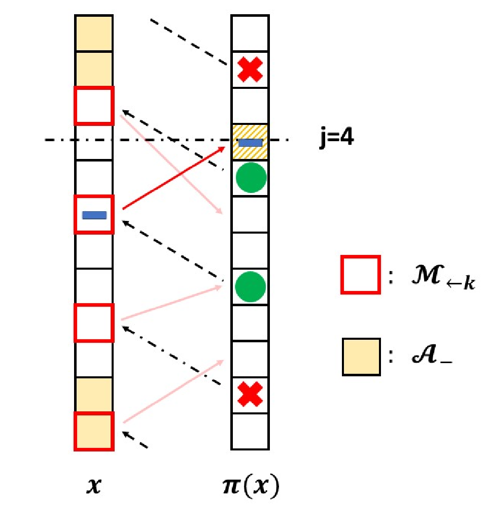
Further denote set $\mathcal{M}=\{\pi(i):\pi(i)\notin\mathcal{B}_{3}\}$ be the collection of indices of initially permuted vector $\pi(\bm{x})$ that are not “ $-$ ” points, and $\mathcal{M}_{\leftarrow k}=(\mathcal{M}-k-1\ mod\ D)+1$ be the corresponding indices shifted backwards. In Figure 14, $\mathcal{M}=\{2,5,8,11\}$ . Also, $\pi(6)=4$ , and the permutation maps are described by the red arrows. Consequently, in $\pi_{\rightarrow k}(\pi(\bm{x}))$ , the $8$ -th element (“ $O$ ”) in $\pi(x)$ will be permuted to the same index of the $8-2=6$ -th element in $\bm{x}$ , which equals to $4$ . It is important to notice that, when considering the $k$ -th collision, only points in $\mathcal{M}_{\leftarrow k}$ matters. Hence, we deduct:

•

(Collision condition) Denote $i=\argmin_{t\in\mathcal{M}_{\leftarrow k}}\pi(\bm{x}_{t})$ be the location of minimal permutation index in $\mathcal{M}_{\leftarrow k}$ . The $k$ -th collision occurs at $j$ i.f.f. $\pi(i)=j$ , and the $i^{*}$ -th element in $\pi(\bm{x})$ must be a “O” point. Recall the definition $i^{*}=(i+k-1\ mod\ D)+1$ .

In Figure 14, consider $i=6$ and $j=4$ for example. Above condition means that the $i=6$ -th element in $\bm{x}$ (“ $-$ ” in red bold border) is permuted to the $j=4$ -th position, and it is above all other permuted elements with red bold borders. Meanwhile, the $i+k=6+2=8$ -th element in $\pi(\bm{x})$ must be a “ $O$ ”. Figure 14 exactly satisfies the condition, so it depicts a collision. Mathematically, we have

	$\displaystyle\mathbb{E}[\mathbbm{1}_{k}]$	$\displaystyle=\sum_{j=1}^{D}P\Big[h_{k}(\bm{v})=h_{k}(\bm{w})=j\Big]$
		$\displaystyle=\sum_{j=1}^{D}\sum_{i=1}^{D}P\Big[\pi(i)=j,\pi^{-1}(i^{*})\in\mathcal{B}_{1}\Big],$		(8)

where $i=\argmin_{t\in\mathcal{M}_{\leftarrow k}}\pi(\bm{x}_{t})$ . In this expression, everything is random of $\pi$ , except for the set $\mathcal{B}_{1}$ which is fixed given the data.

Now we will focus on deriving the probability for a fixed $i$ and $j$ in (8). Our analysis will be conditional on the collection of variables $Z$ which is defined as follows. Let $z_{-,1}$ , $z_{-,2}$ and $z_{-,3}$ be the number of “ $O$ ”, “ $\times$ ” and “ $-$ ” points in $\mathcal{A}_{-}(j)\cap\mathcal{M}_{\leftarrow k}^{c}$ , and $z_{+,1}$ , $z_{+,2}$ and $z_{+,3}$ be the number of “ $O$ ”, “ $\times$ ” and “ $-$ ” points in $\mathcal{A}_{+}(j)\cap\mathcal{M}_{\leftarrow k}^{c}$ , respectively. Here $\mathcal{M}_{\leftarrow k}^{c}$ represents the complement of $\mathcal{M}_{\leftarrow k}$ . Notice that $Z$ (and its density function) depends on different $j$ since $\mathcal{A}_{-}(j)$ and $\mathcal{A}_{+}(j)$ depends on $j$ . For the ease of notation we suppress the information of $j$ in $Z$ (and $z$ ’s). It is easy to see that $Z=(z_{-,k}|_{1}^{3},z_{+,k}|_{1}^{3})$ follows hyper( $D,D-f,n_{-,k}(j)|_{1}^{3},n_{+,k}(j)|_{1}^{3}$ ). Denote the domain of $Z$ and $\Theta_{j}$ . Conditional on $Z$ , we obtain

$\displaystyle\mathbb{E}[\mathbbm{1}_{k}]$	$\displaystyle=\sum_{j=1}^{D}\sum_{Z\in\Theta_{j}}\sum_{i=1}^{D}P\Big[\pi(i)=j,\pi^{-1}(i^{*})\in\mathcal{B}_{1}\|Z\Big]P_{j}\Big[Z\Big]$
	$\displaystyle=\sum_{j=1}^{D}\sum_{Z\in\Theta_{j}}\sum_{i=1}^{D}P\Big[\pi^{-1}(i^{*})\in\mathcal{B}_{1}\|\pi(i)=j,Z\Big]P\Big[\pi(i)=j\|Z\Big]P_{j}\Big[Z\Big]$
	$\displaystyle\triangleq\sum_{j=1}^{D}\sum_{Z\in\Theta_{j}}\sum_{i=1}^{D}\Gamma(i,j)P_{j}\Big[Z\Big],$	(9)

with $i=\argmin_{t\in\mathcal{M}_{\leftarrow k}}\pi(\bm{x}_{t})$ . We will carefully compute the probabilities in the summation. Basically, the key is that elements in $\mathcal{M}$ need to be controlled, i.e. smaller than $j$ , and other positions can be arbitrary. Given $Z$ , this means that we need to put $r_{1}=a-z_{-,1}-z_{+,1}$ type “ $O$ ” points, $r_{2}=f-a-z_{-,2}-z_{+,2}$ type “ $\times$ ” points and $r_{3}=D-f-z_{-,3}-z_{+,3}$ type “ $-$ ” points no smaller than $j$ , with $\pi(i)=j$ exactly. Also note that there are fixed $b_{0}=\sum_{k=1}^{3}z_{+,k}$ type “ $-$ ” points no smaller than $j$ .

With all these definitions and reasoning, we are ready to proceed with the proof. Based on $\bm{x}_{i}$ , we have three general cases.

1) $\bm{x}_{i}\in\mathcal{B}_{1}$ . The first case is that $\bm{x}_{i}=O$ .

Case 1a) $j<i^{*}$ . Firstly, we consider the case where $j<i^{*}$ . By combinatorial theory we have

$\displaystyle P\Big[\pi(i)=j\|Z\Big]$	$\displaystyle=P\Big[\pi(i)=j\|\pi^{-1}(j)\notin\mathcal{B}_{3},Z\Big]P\Big[\pi^{-1}(j)\notin\mathcal{B}_{3}\|Z\Big]$
	$\displaystyle=\frac{1}{r_{1}+r_{2}}\frac{\binom{b_{0}}{r_{3}}\binom{D-j-b_{0}}{r_{1}+r_{2}-1}}{\binom{D-f}{r_{3}}\binom{f}{r_{1}+r_{2}}}P\Big[\pi^{-1}(j)\notin\mathcal{B}_{3}\|Z\Big]$
	$\displaystyle\triangleq\tilde{P}_{1}\cdot P\Big[\pi^{-1}(j)\notin\mathcal{B}_{3}\|Z\Big],$	(10)

where the second probability is that the $j$ -th element in $\pi(\bm{x})$ is not “ $-$ ”. Conditional on $Z$ , the probability is dependent on $j^{\#}$ :

\displaystyle P\Big[\pi^{-1}(j)\notin B_{3}|Z\Big]=\sum_{p=1}^{3}\mathbbm{1}\{j^{\#}\in\mathcal{B}_{p}\}(1-\frac{z_{-,p}}{n_{-,p}(j)}).

Combining with (10) we obtain

\displaystyle P\Big[\pi(i)=j|Z\Big]=\tilde{P}_{1}\sum_{p=1}^{3}\mathbbm{1}\{j^{\#}\in\mathcal{B}_{p}\}(1-\frac{z_{-,p}}{n_{-,p}(j)}).

(11)

Next we compute $P[\pi^{-1}(i^{*})\in\mathcal{B}_{1}|\pi(i)=j,Z]$ . Note that given the conditions, $\pi^{-1}(i^{*})$ has two cases: 1) it comes from $\mathcal{M}_{\leftarrow k}$ (i.e. it is one of the elements with red bold border); 2) Otherwise. We then can write

		$\displaystyle P\Big[\pi^{-1}(i^{*})\in\mathcal{B}_{1}\|\pi(i)=j,Z\Big]$
		$\displaystyle=P\Big[\pi^{-1}(i^{})\in\mathcal{B}_{1}\|\pi^{-1}(i^{})\in\mathcal{M}_{\leftarrow k},\pi(i)=j,Z\Big]P\Big[\pi^{-1}(i^{*})\in\mathcal{M}_{\leftarrow k}\|\pi(i)=j,Z\Big]$
		$\displaystyle\hskip 36.135pt+P\Big[\pi^{-1}(i^{})\in\mathcal{B}_{1}\|\pi^{-1}(i^{})\notin\mathcal{M}_{\leftarrow k},\pi(i)=j,Z\Big]P\Big[\pi^{-1}(i^{*})\notin\mathcal{M}_{\leftarrow k}\|\pi(i)=j,Z\Big]$
		$\displaystyle=(1-\frac{z_{+,1}}{n_{+,1}(j)})\left[\frac{r_{1}+r_{2}-1}{D-j-b_{0}}\frac{r_{1}-1}{r_{1}+r_{2}-1}+(1-\frac{r_{1}+r_{2}-1}{D-j-b_{0}})\frac{a-r_{1}}{f-r1-r2}\right]$
		$\displaystyle\triangleq(1-\frac{z_{+,1}}{n_{+,1}(j)})\left[\frac{r_{1}-1}{D-j-b_{0}}+(1-\frac{r_{1}+r_{2}-1}{D-j-b_{0}})J^{*}\right]$
		$\displaystyle\triangleq(1-\frac{z_{+,1}}{n_{+,1}(j)})\bar{J}_{1}.$		(12)

Combining (11) and (12), we obtain when $i\in\mathcal{B}_{1}$ and $j<i^{*}$ ,

\displaystyle\Gamma(i,j)=\sum_{p=1}^{3}\mathbbm{1}\{j^{\#}\in\mathcal{B}_{p}\}(1-\frac{z_{-,p}}{n_{-,p}(j)})(1-\frac{z_{+,1}}{n_{+,1}(j)})\tilde{P}_{1}\bar{J}_{1}.

(13)

Case 1b) $j=i^{*}$ . Similarly approach also applies to the situation with $j=i^{*}$ . In this case,

\displaystyle P\Big[\pi^{-1}(j)\notin\mathcal{B}_{3}|Z\Big]=(1-\frac{z_{-,1}}{n_{-,1}(j)})\tilde{P}_{1},\hskip 14.45377ptP[\pi^{-1}(i^{*})\in\mathcal{B}_{1}|\pi(i)=j,Z]=1.

(14)

The equations are because $(i^{*})^{\#}=i\in\mathcal{B}_{1}$ , and equivalently, $\pi^{-1}(i^{*})=\pi^{-1}(j)=i\in\mathcal{B}_{1}$ .

Case 1c) $j>i^{*}$ . I this case, we still have

\displaystyle P\Big[\pi(i)=j|Z\Big]=\tilde{P}_{1}\sum_{p=1}^{3}\mathbbm{1}\{j^{\#}\in\mathcal{B}_{p}\}(1-\frac{z_{-,p}}{n_{-,p}(j)}),

but the probability of $\pi_{-1}(i^{*})$ being “ $O$ ” is different. Since $j>i^{*}$ , this event now depends on $z_{-,p}$ , $p=1,2,3$ . More specifically,

		$\displaystyle P[\pi^{-1}(i^{*})\in\mathcal{B}_{1}\|\pi(i)=j,Z]$
		$\displaystyle=\left[\mathbbm{1}\{j^{\#}\in\mathcal{B}_{1}\}(1-\frac{z_{-,1}}{n_{-,1}(j)-1})+\sum_{p=2,3}\mathbbm{1}\{j^{\#}\in\mathcal{B}_{p}\}(1-\frac{z_{-,p}}{n_{-,p}(j)})\right]J^{*}.$

Therefore, when $i\in\mathcal{B}_{1}$ and $j>j^{*}$ , it holds that

\displaystyle\Gamma(i,j)=(1-\frac{z_{-,1}}{n_{-,1}(j)})\left[\mathbbm{1}\{j^{\#}\in\mathcal{B}_{1}\}(1-\frac{z_{-,1}}{n_{-,1}(j)-1})+\sum_{p=2,3}\mathbbm{1}\{j^{\#}\in\mathcal{B}_{p}\}(1-\frac{z_{-,p}}{n_{-,p}(j)})\right]J^{*}.

(15)

2) $\bm{x}_{i}\in\mathcal{B}_{2}$ . The case where $\bm{x}_{i}\in\mathcal{B}_{2}$ can be analyzed using similar arguments. For conciseness, we mainly present the final results.

Case 2a) $j<i^{*}$ . The calculation ends up in the same form. We have

\displaystyle P\Big[\pi(i)=j|Z\Big]=\tilde{P}_{2}\sum_{p=1}^{3}\mathbbm{1}\{j^{\#}\in\mathcal{B}_{p}\}(1-\frac{z_{-,p}}{n_{-,p}(j)}),

with $\tilde{P}_{2}=\tilde{P}_{1}$ . In addition,

\displaystyle P\Big[\pi^{-1}(i^{*})\in\mathcal{B}_{1}|\pi(i)=j,Z\Big]=(1-\frac{z_{+,2}}{n_{+,2}(j)})\bar{J}_{2},

where $\bar{J}_{2}=\frac{r_{1}}{D-j-b_{0}}+(1-\frac{r_{1}+r_{2}-1}{D-j-b_{0}})J^{*}$ . Hence, when $\bm{x}_{i}\in\mathcal{B}_{2}$ and $j<i^{*}$ , we have

\displaystyle\Gamma(i,j)=\sum_{p=1}^{3}\mathbbm{1}\{j^{\#}\in\mathcal{B}_{p}\}(1-\frac{z_{-,p}}{n_{-,p}(j)})(1-\frac{z_{+,2}}{n_{+,2}(j)})\tilde{P}_{2}\bar{J}_{2}.

(16)

Case 2b) $j=i^{*}$ . In this case, $\Gamma(i,j)$ simply equals to $0$ , since $\pi^{-1}(i^{*})=\pi^{-1}(j)\in\mathcal{B}_{2}$ . The probability of $\pi^{-1}(i^{*})$ being “ $O$ ” is $0$ .

Case 2c) $j>i^{*}$ . Omitting the details, we have

\displaystyle\Gamma(i,j)=(1-\frac{z_{-,2}}{n_{-,2}(j)})\left[\mathbbm{1}\{j^{\#}\in\mathcal{B}_{2}\}(1-\frac{z_{-,2}}{n_{-,2}(j)-1})+\sum_{p=1,3}\mathbbm{1}\{j^{\#}\in\mathcal{B}_{p}\}(1-\frac{z_{-,p}}{n_{-,p}(j)})\right]J^{*}.

(17)

2) $\bm{x}_{i}\in\mathcal{B}_{3}$ .

Case 3a) $j<i^{*}$ . The expression is different from previous two, in that we need $\pi^{-1}(j)\in B_{3}$ .

	$\displaystyle P\Big[\pi(i)=j\|Z\Big]$	$\displaystyle=P\Big[\pi(i)=j\|\pi^{-1}(j)\in B_{3},Z\Big]P\Big[\pi^{-1}(j)\in B_{3}\|Z\Big]$
		$\displaystyle=\tilde{P}_{3}\sum_{p=1}^{3}\mathbbm{1}\{j^{\#}\in\mathcal{B}_{p}\}\frac{z_{-,p}}{n_{-,p}(j)},$

where

\displaystyle\tilde{P}_{3}=\frac{1}{r_{3}}\frac{\binom{b_{0}}{r_{3}-1}\binom{D-j-b_{0}}{r_{1}+r_{2}}}{\binom{D-f}{r_{3}}\binom{f}{r_{1}+r_{2}}}.

Moreover, we have

\displaystyle P\Big[\pi^{-1}(i^{*})\in\mathcal{B}_{1}|\pi(i)=j,Z\Big]=(1-\frac{z_{+,3}}{n_{+,3}(j)})\bar{J}_{3},

with $\bar{J}_{3}=\frac{r_{1}}{D-j-b_{0}}+(1-\frac{r_{1}+r_{2}}{D-j-b_{0}})J^{*}$ . Combining parts together we obtain

\displaystyle\Gamma(i,j)=\sum_{p=1}^{3}\mathbbm{1}\{j^{\#}\in\mathcal{B}_{p}\}\frac{z_{-,p}}{n_{-,p}(j)}(1-\frac{z_{+,3}}{n_{+,3}(j)})\tilde{P}_{3}\bar{J}_{3}.

(18)

Case 3b) $j=i^{*}$ . By same reasoning as Case 2a), $\Gamma(i,j)=0$ .

Case 3c) $j>i^{*}$ . We have in this case

	$\displaystyle\Gamma(i,j)$	$\displaystyle=\left[\mathbbm{1}\{j^{\#}\in\mathcal{B}_{3}\}\frac{z_{-,3}}{n_{-,3}(j)}\frac{n_{-,3}(j)-z_{-,3}}{n_{-,3}(j)-1}+(1-\frac{z_{-,3}}{n_{-,3}(j)})\sum_{p=1,2}\mathbbm{1}\{j^{\#}\in\mathcal{B}_{p}\}\frac{z_{-,p}}{n_{-,p}(j)}\right]J^{*}$
		$\displaystyle=\sum_{p=1}^{3}\mathbbm{1}\{j^{\#}\in\mathcal{B}_{p}\}\frac{z_{-,p}}{n_{-,p}(j)}(1-\frac{z_{-,3}-\mathbbm{1}\{p=3\}}{n_{-,3}(j)}-\mathbbm{1}\{p=3\})J^{*}.$		(19)

Finally, combining (9), (13), (14), (15), (16), (17), (18) and (19), and re-organizing terms, the proof is complete.

∎

References

Broder (1997) Andrei Z. Broder. On the resemblance and containment of documents. In Proceedings of the Conference on Compression and Complexity of SEQUENCES, pages 21–29, Positano, Amalfitan Coast, Salerno, Italy, 1997.
Broder et al. (1997) Andrei Z. Broder, Steven C. Glassman, Mark S. Manasse, and Geoffrey Zweig. Syntactic clustering of the web. Comput. Networks, 29(8-13):1157–1166, 1997.
Broder et al. (1998) Andrei Z. Broder, Moses Charikar, Alan M. Frieze, and Michael Mitzenmacher. Min-wise independent permutations. In Proceedings of the Thirtieth Annual ACM Symposium on the Theory of Computing (STOC), pages 327–336, Dallas, TX, 1998.
Chang and Lin (2011) Chih-Chung Chang and Chih-Jen Lin. LIBSVM: A library for support vector machines. ACM Transactions on Intelligent Systems and Technology, 2:27:1–27:27, 2011.
Dua and Graff (2017) Dheeru Dua and Casey Graff. UCI machine learning repository, 2017. URL http://archive.ics.uci.edu/ml.
Greene and Cunningham (2006) Derek Greene and Pádraig Cunningham. Practical solutions to the problem of diagonal dominance in kernel document clustering. In Proc. 23rd International Conference on Machine learning (ICML’06), pages 377–384. ACM Press, 2006.
Krizhevsky (2009) Alex Krizhevsky. Learning multiple layers of features from tiny images. 2009.
LeCun et al. (1998) Yann LeCun, Léon Bottou, Yoshua Bengio, and Patrick Haffner. Gradient-based learning applied to document recognition. Proceedings of the IEEE, 86(11):2278–2324, 1998.
Li and Church (2005) Ping Li and Kenneth Ward Church. Using sketches to estimate associations. In Proceedings of the Conference on Human Language Technology and the Conference on Empirical Methods in Natural Language Processing (HLT/EMNLP), pages 708–715, Vancouver, Canada, 2005.
Li and König (2011) Ping Li and Arnd Christian König. Theory and applications of b-bit minwise hashing. Commun. ACM, 54(8):101–109, 2011.
Li and Li (2021) Xiaoyun Li and Ping Li. C-MinHash: Rigorously reducing $k$ permutations to two. arXiv preprint arXiv:2109.03337, 2021.

$\displaystyle P\Big[\pi(i)=j\|Z\Big]$	$\displaystyle=P\Big[\pi(i)=j\|\pi^{-1}(j)\notin\mathcal{B}_{3},Z\Big]P\Big[\pi^{-1}(j)\notin\mathcal{B}_{3}\|Z\Big]$
	$\displaystyle=\frac{1}{r_{1}+r_{2}}\frac{\binom{b_{0}}{r_{3}}\binom{D-j-b_{0}}{r_{1}+r_{2}-1}}{\binom{D-f}{r_{3}}\binom{f}{r_{1}+r_{2}}}P\Big[\pi^{-1}(j)\notin\mathcal{B}_{3}\|Z\Big]$
	$\displaystyle\triangleq\tilde{P}_{1}\cdot P\Big[\pi^{-1}(j)\notin\mathcal{B}_{3}\|Z\Big],$	(10)

C-MinHash: Practically Reducing Two Permutations to Just One

Abstract

1 Background

2 Review of MinHash and C-MinHash

Theorem 2.1.

3 C-MinHash-(π,π)(\pi,\pi): Reducing Two Permutations to Just One

Definition 3.1.

Theorem 3.1.

4 Further Empirical Verification

4.1 MSE Comparisons on Words Dataset

4.2 Comparing Estimation Errors in All Pairs for Several Datasets

5 Conclusion

Appendix A Proof of Theorem 3.1

Proof.

References

C-MinHash:
Practically Reducing Two Permutations to Just One

3 C-MinHash- $(\pi,\pi)$ : Reducing Two Permutations to Just One