Detection of Abrupt Change in Channel Covariance Matrix for Multi-Antenna Communication

In modern wireless systems, multiple-input multiple-output (MIMO) is a core technology to improve the channel capacity and reliability. However, the MIMO beamforming design crucially relies on the knowledge of the channel state information. Along this line, many efficient algorithms have been proposed to estimate the user instantaneous channels [1, 2].

In practice, user channels are spatially correlated due to the dependent antenna patterns at the base station (BS) and the finite number of scatters [3, 4]. In this case, the acquisition of the channel covariance matrices is important as well. On one hand, to estimate the instantaneous channels, we need to estimate the channel covariance matrices first, because the minimum mean-squared error (MMSE) channel estimators are usually functions of the channel covariance matrices [5]. On the other hand, there is a new trend to design the beamforming vectors based on the channel covariance matrices [6, 7, 8], instead of the instantaneous channels. This is because channel covariance matrices change much more slowly than instantaneous channels, and the overhead to estimate these matrices is thus much lower. Such a property is especially appealing for downlink massive MIMO systems [5, 9, 10] and intelligent reflecting surface (IRS) systems [11, 12, 13], where the overhead for estimating so many channel coefficients in each coherence block is huge [14, 15]. Motivated by the above reasons, several interesting works have been done on channel covariance matrix estimation [16, 17].

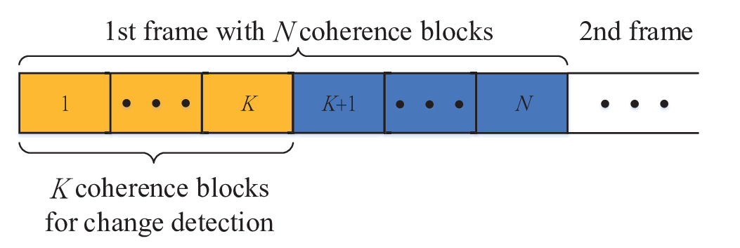
Despite slowly, the channel covariance matrices do vary in practice due to the change in the environment and the user location. A key question is when an abrupt change occurs, how to detect it accurately and quickly such that we can re-estimate the channel covariance matrices as soon as possible. In this paper, we focus on this challenge in a point-to-point communication system, where a multi-antenna BS serves a single-antenna user equipment (UE). A novel change detection protocol is proposed as shown in Fig. 1, where a proper number of coherence blocks form a frame, and the pilot signals received across a small number of blocks at the beginning of each frame will be used to detect whether the channel covariance matrix changes over the previous frame. The complicated approaches proposed in [16, 17] will be only adopted to estimate the channel covariance matrix in the subsequent blocks when a change is detected.

Under this protocol, an intuitive way for change detection is to first estimate the new covariance matrix very accurately and then compare it with the previous one. However, a precise estimation usually requires pilot signals over a sufficiently long time, making quick change detection impossible. In this paper, we apply the classic change detection theory [18] to tackle this issue. First, we propose a genie-aided change detector based on the log-likelihood (LLR) test, where the covariance matrix after change is assumed to be known. The probabilities of missed detection and false alarm are characterized, which can sever as performance limit. Then, we consider the practical case without knowledge of the covariance matrix in the new frame. Maximum likelihood (ML) technique is used to estimate the new covariance matrix, and the LLR-based change detector is then proposed based on the estimated covariance matrix. Numerical results show that our proposed scheme can achieve very low probabilities of missed detection and false alarm even when the number of detection blocks is small, because a moderate (instead of exact) estimation of the covariance matrix is a sufficient evidence under our proposed change detector.

Consider a narrow-band communication system where a BS equipped with $M$ antennas serves a single-antenna UE. We assume a block fading channel model, where channel stays constant in one coherence block, but may vary independently over different blocks. Let $\boldsymbol{h}\in\mathbb{C}^{M\times 1}$ denote the channel between the BS and the UE. In this paper, we consider a Rayleigh fading channel model, i.e., $\boldsymbol{h}\sim\mathcal{CN}(\boldsymbol{0},\boldsymbol{C}^{h})$, where $\boldsymbol{C}^{h}$ denotes the covariance matrix of $\boldsymbol{h}$. In practice, $\boldsymbol{C}^{h}$ changes much more slowly than $\boldsymbol{h}$. Our aim is to detect the change in $\boldsymbol{C}^{h}$ accurately and quickly.

To realize this goal, in this paper, we propose a novel change detection protocol, as shown in Fig. 1, which can be applied in both downlink and uplink communication. First, we define a frame as the collection of $N$ coherence blocks. In practice, we can measure the average frequency for the occurrence of the change in $\boldsymbol{C}^{h}$ and set $N$ properly based on this frequency such that $\boldsymbol{C}^{h}$ will change at most once over one frame. Then, based on the pilot signals received at the first $K$ coherence blocks of each frame, the system needs to determine whether the channel covariance matrix in the current frame, denoted by $\boldsymbol{C}^{h}_{1}$, is the same as that in the previous frame, denoted by $\boldsymbol{C}_{0}^{h}$. In other words, we need to detect between two hypothesis

If a change has been detected, i.e., $H_{1}$ is true, we can use more coherence blocks following the first $K$ coherence blocks to estimate the new channel covariance matrix $\boldsymbol{C}^{h}_{1}$ based on the existing techniques [19, 16, 17]. Otherwise, if $H_{0}$ is true, the estimated covariance matrix remains the same as that in the previous frame. As a result, at any frame, we always know the channel covariance matrix in the previous frame. In the rest of this paper, we focus on how to perform change detection based on the pilot signals received at the first $K$ coherence blocks of each frame, with the prior knowledge of channel covariance matrix in the previous frame.

Specifically, at the $k$-th coherence block of a frame, $1\leq k\leq K$, the received pilot signals in the uplink and downlink are respectively give as

where $\boldsymbol{h}_{k}\backsim\mathcal{CN}(\boldsymbol{0},\boldsymbol{C}^{h}_{1})$ denotes the channel at the $k$-th block of the considered frame, $\rho$ denotes the transmit power, $\boldsymbol{x}\in\mathbb{C}^{T\times 1}$ and $\boldsymbol{X}\in\mathbb{C}^{T\times M}$ denote the uplink and downlink pilot signals with length $T$, and $\boldsymbol{N}^{{\rm ul}}_{k}\in\mathbb{C}^{M\times T}\backsim\mathcal{CN}(\boldsymbol{0},\sigma^{2}\boldsymbol{I})$ and $\boldsymbol{n}^{{\rm dl}}_{k}\backsim\mathcal{CN}(\boldsymbol{0},\sigma^{2}\boldsymbol{I})$ denote the additive white Gaussian noise (AWGN) at the BS side and the UE side. In the uplink, the pilot sequence satisfies $\boldsymbol{x}^{H}\boldsymbol{x}=T$, while in the downlink, we assume that the pilot sequence length satisfies $T\geq M$ such that $\boldsymbol{X}^{H}\boldsymbol{X}=T\boldsymbol{I}$.

One intuitive way to perform change detection is to first estimate $\boldsymbol{C}_{1}^{h}$ very accurately and then detect whether a change has occurred in $\boldsymbol{C}_{0}^{h}$. However, an accurate estimation of $\boldsymbol{C}_{1}^{h}$ depends on: 1. an accurate estimation of $\boldsymbol{h}_{k}$ at each coherence block via some advanced signal processing technique; and 2. a sufficiently large number of samples about $\boldsymbol{h}_{k}$’s. However, advanced channel estimation techniques, e.g., MMSE estimation, usually require the channel statistical information, which is not available here because we do not know whether the channel covariance matrix is still $\boldsymbol{C}_{0}^{h}$. Moreover, in practice, any change should be detected within a short time duration, and an accurate estimation of $\boldsymbol{C}_{1}^{h}$ over a longer time duration is only performed after (not before) a change is detected.

To address the above issues under the protocol shown in Fig. 1, this paper proposes the following change detection scheme. First, the channel at each coherence block of the phase detection phase is estimated based on the ML technique¹¹ 1 After the change detection phase in the frame, Bayesian channel estimation techniques, e.g., MMSE estimation, can be applied based on the new channel statistics to replace the ML estimation for reducing estimation mean-squared error., which requires no statistical information of the channel. For the received pilot signals (2) and (3), the ML channel estimators at coherence block $k$ in the uplink and downlink can be unified as

where $\tilde{\boldsymbol{n}}_{k}\backsim\mathcal{CN}(\boldsymbol{0},\frac{\sigma^{2}}{E_{0}}\boldsymbol{I})$ with $E_{0}=\rho T$. Second, after the ML channel estimators in the $K$ coherence blocks, denoted by $\tilde{\boldsymbol{H}}=[\tilde{\boldsymbol{h}}_{1},...,\tilde{\boldsymbol{h}}_{K}]\in\mathbb{C}^{T\times K}$, are obtained, we aim to apply the LLR test based on the change detection theory [18] such that a change can be detected accurately just utilizing a small number of channel samples.

To introduce the change detection theory [18] and provide performance upper bound, in the following, we first focus on how to perform LLR test in the ideal case that if there is a change of the channel covariance matrix in the current frame, the new covariance matrix is a known matrix $\boldsymbol{C}_{1}^{h}\neq\boldsymbol{C}_{0}^{h}$. Then, we will focus on LLR test for change detection in the practical scenario where the channel covariance matrix in the current frame $\boldsymbol{C}_{1}^{h}$ is unknown and needs to be estimated roughly first.

In this section, we consider the practical scenario where $\boldsymbol{C}_{1}^{h}$ is unknown. Different from the ideal case that $\boldsymbol{C}_{1}^{h}$ is known, we will first estimate $\boldsymbol{C}_{1}^{h}$ roughly based on $\tilde{\boldsymbol{H}}$ (4) by using the ML technique, based on which the LLR-based detector is then used to detect whether a change occurs.

Specifically, according to the change detector (11), the ML estimator of $\boldsymbol{C}_{1}^{h}$ given $\tilde{\boldsymbol{H}}$ is defined as the covariance matrix that can maximize the sum of the log-likelihood over the $K$ coherence blocks, i.e.,

where $\tilde{S}(\tilde{\boldsymbol{H}},\boldsymbol{C}_{1}^{h})$ is given in (9). As shown in [22], the optimal solution to (17) is $\hat{\boldsymbol{C}}_{1}^{h}=\boldsymbol{S}_{\tilde{H}}-\frac{\sigma^{2}}{E_{0}}\boldsymbol{I}$, where $\boldsymbol{S}_{\tilde{H}}$ is the sample covariance matrix given in (10).

However, when $K\ll M$, the ML estimator based on the sample covariance matrix is ill-conditioned. To improve the estimation performance, we introduce new constraints to problem (17) for reducing the condition number of the estimated covariance matrix. Specifically, the modified problem to obtain the ML estimator of $\boldsymbol{C}_{1}^{h}$ is given by

where $\beta>0$ and $\kappa\beta$ with $\kappa>1$ are the lower bound and upper bound for the minimum eigenvalue and the maximum eigenvalue, respectively, to ensure that the estimated covariance matrix is well-conditioned. It is non-trivial to solve Problem $\mathcal{P}_{1}$, because it is non-convex. However, in the following, we manage to characterize its closed-form solution.

In this section, we present numerical results to verify the effectiveness of the proposed change detectors. Due to the space limitations, we just consider downlink in the simulation. All relevant simulation parameters are given in Table I. Specifically, the BS has $M=32$ antennas, while the pilot sequence length in the considered $K$ coherence blocks is set to be $T=M=32$. The pilot sequence $\boldsymbol{X}$ is generated based on the discrete Fourier transform (DFT) matrix. The carrier frequency is selected as a typical E-band mmWave frequency at 80$\mathrm{GHz}$. We set the signal-to-noise ratio (SNR) for the communication between the BS and the UE as $0\textup{dB}$. Moreover, we use the “one-ring” model to describe the covariance matrix of the UE channel, which is shown in (31) at the top of next page. Particularly, $\boldsymbol{C}_{m1,m2}^{h}$ denotes the element at the $m1$-th row and $m2$-th column of $\boldsymbol{C}^{h}$, $\Omega$ denotes the angle of departure (AoD), $\Psi$ denotes the angle spread, $\alpha$ denotes the wavelength of the signal, $D_{m1,m2}=2(m1-m2)\alpha$ is the relative spacing distance between antenna $m1$ and antenna $m2$, and $\theta$ denotes the angle of a possible scatter around the UE. In the rest of this section, we assume that the change in the channel covariance matrix is caused by the change of AoD. We use $\Delta\Omega$ to denote the change of AoD.

First, we illustrate the performance of the genie-aided change estimator when $\boldsymbol{C}_{1}^{h}$ is known. Fig. 2 shows the detection error probability as given in (12) versus the number of detection coherence blocks when $\Delta\Omega=0.1^{\circ},0.5^{\circ},1^{\circ}$, respectively. Particularly, we select the threshold $\Theta$ such that the probabilities of false alarm and missed detection are the same. First, it is observed that the error probability obtained via Monte Carlo simulation matches perfectly with that from Theorem 1. Next, it is observed that when $\boldsymbol{C}_{1}^{h}$ is known, very good change detection accuracy can be obtained even when $K$ is much smaller than $M$. Last, it is observed that the detection accuracy increases when the change in the channel covariance matrix is more significant.

Next, we consider the case when $\boldsymbol{C}_{1}^{h}$ is unknown. We adopt the following benchmark scheme.

Benchmark Scheme (Shrinkage-based Estimation): Based on the shrinkage technique in [19], the estimation of $\boldsymbol{C}^{h}_{1}$ can be expressed as

where $0\leq\rho\leq 1$ is the shrinkage parameter to define the weight of the sample covariance matrix in the estimation. According to [19], a good choice of $\rho$ is

Based on (11), the change detector under the shrinkage estimation of $\boldsymbol{C}_{1}^{h}$ is given by

Fig. 3 shows the performance comparison between the change detectors based on the ML estimation and shrinkage-based estimation of $\boldsymbol{C}_{1}^{h}$ when $K=30<M$ and $\Delta\Omega=0.75^{\circ}$. By varying the threshold $\Theta$, we can get the whole trade-off between the false alarm probability and missed detection probability. Firstly, it is observed that even if $\boldsymbol{C}_{1}^{h}$ is unknown, the error probability of our proposed change detectors is quite low. Secondly, it is observed that changed detector based on the ML estimation performs better than the change detector based on the shrinkaged-based estimation when $K<M$. Thirdly, it is observed that the change detector based on the ML-based estimation with $\kappa=4$ performs better than that with $\kappa=6$, while performs worse than that with $\kappa=3$, which indicates that an appropriate constraint on the condition number of $\hat{\boldsymbol{C}}_{h}^{1}$ is demanded to guarantee high performance of the proposed ML estimation.

We further study the performance of the changed detectors based on the ML estimation and the shrinkage estimation when $K>M$. Fig. 4 shows the performance comparison of these two change detectors when $\Delta\Omega$ is reduced from $0.75^{\circ}$ to $0.5^{\circ}$ such that events of false alarm and missed detection can be observed in our Monte Carlo simulation with larger $K$. It is observed that when $K$ increases from $50$ to $100$, the performance gap between the ML estimation based change detector and the shrinkage estimation based change detector becomes larger. However, as $K$ becomes larger and larger, the performance gap will vanish because at last, both the ML estimation and the shrinkage estimation will lead to very accurate estimation when $K$ is sufficiently large. We do not show this result since when $K$ is very large, the error probability is very low and no false alarm and missed detection events are observed in our Monte Carlo simulation.

In this paper, we studied channel covariance change detection in a system consisting of a multi-antenna BS and a single-antenna UE. First, we proposed a genie-aided change detector based on the LLR test, assuming that the knowledge of the new channel covariance matrix is known. The probabilities of false alarm and missed detection were characterized, which may serve as performance limit. Then, we considered the practical scenario with unknown new channel covariance matrix and proposed an LLR-based change detector based on the ML estimation technique. Numerical results that when the new channel covariance matrix is unknown, our proposed strategies can detect the change very accurately even with a small number of samples.

References

- [1] B. Hassibi and B. M. Hochwald, “How much training is needed in multiple-antenna wireless links,” IEEE Trans. Inf. Theory, vol. 49, no. 4, pp. 951–963, Apr. 2013.
- [2] M. Biguesh and A. B. Gershman, “Training-based MIMO channel estimation: A study of estimator tradeoffs and optimal training signals,” IEEE Trans. Signal Process.,, vol. 54, no. 3, pp. 884–893, Mar. 2006.
- [3] X. Gao, O. Edfors, F. Rusek, and F. Tufvesson, “Massive MIMO performance evaluation based on measured propagation data,” IEEE Trans. Wireless Commun., vol. 14, no. 7, pp. 3899–3911, Jul. 2015.
- [4] L. Sanguinetti, E. Björnson, and J. Hoydis, “Toward massive MIMO 2.0: Understanding spatial correlation, interference suppression, and pilot contamination,” IEEE Trans. Commun., vol. 68, no. 1, pp. 232–257, Jan. 2020.
- [5] T. L. Marzetta, E. G. Larsson, H. Yang, and H. Q. Ngo, Fundamentals of massive MIMO. Cambridge, U.K.: Cambridge Univ. Press, 2016.
- [6] S. Park, J. Park, A. Yazdan, and R. W. Heath, “Exploiting spatial channel covariance for hybrid precoding in massive MIMO systems,” IEEE Trans. Signal Process., vol. 65, no. 14, pp. 3818–3832, Jul. 2017.
- [7] Y. Han, W. Tang, S. Jin, C.-K. Wen, and X. Ma, “Large intelligent surface-assisted wireless communication exploiting statistical CSI,” IEEE Trans. Veh. Technol., vol. 68, no. 8, pp. 8238–8242, Aug. 2019.
- [8] M.-M. Zhao, Q. Wu, M.-J. Zhao, and R. Zhang, “Intelligent reflecting surface enhanced wireless network: Two-timescale beamforming optimization,” IEEE Trans. Wireless Commun., vol. 20, no. 1, pp. 2–17, Jan. 2021.
- [9] T. L. Marzetta, “Noncooperative cellular wireless with unlimited numbers of base station antennas,” IEEE Trans. Wireless Commun., vol. 9, no. 11, pp. 3590–3600, Oct. 2010.
- [10] E. G. Larsson, O. Edfors, F. Tufvesson, and T. L. Marzetta, “Massive MIMO for next generation wireless systems,” IEEE commun. mag., vol. 52, no. 2, pp. 186–195, Feb. 2014.
- [11] C. Liaskos, S. Nie, A. Tsioliaridou, A. Pitsillides, S. Ioannidis, and I. Akyildiz, “A new wireless communication paradigm through software-controlled metasurfaces,” IEEE Commun. Mag., vol. 56, no. 9, pp. 162–169, Sep. 2018.
- [12] M. D. R. et al., “Smart radio environments empowered by reconfigurable AI meta-surfaces: An idea whose time has come,” EURASIP J. Wireless Commun. Network., no. 129, pp. 1–20, May 2019.
- [13] Q. Wu, S. Zhang, B. Zheng, C. You, and R. Zhang, “Intelligent reflecting surface aided wireless communications: A tutorial,” IEEE Trans. Commun., vol. 69, no. 5, pp. 3313–3351, May 2021.
- [14] E. Björnson, E. G. Larsson, and T. L. Marzetta, “Massive MIMO: Ten myths and one critical question,” IEEE Commun. Mag., vol. 54, no. 2, pp. 114–123, Feb. 2016.
- [15] Z. Wang, L. Liu, and S. Cui, “Channel estimation for intelligent reflecting surface assisted multiuser communications: Framework, algorithms, and analysis,” IEEE Trans. Wireless Commun, vol. 19, no. 10, pp. 6607–6620, Oct. 2020.
- [16] Y.-C. Liang and F. P. S. Chin, “Downlink channel covariance matrix (DCCM) estimation and its applications in wireless DS-CDMA systems,” IEEE J. Select. Areas Commun., vol. 19, no. 2, pp. 222–232, Feb. 2001.
- [17] K. Upadhya and S. A. Vorobyov, “Covariance matrix estimation for massive MIMO,” IEEE Signal Process. Lett., vol. 25, no. 4, pp. 546–550, Feb. 2018.
- [18] M. Basseville, I. V. Nikiforov et al., Detection of abrupt changes: Theory and application. Prentice hall Englewood Cliffs, 1993, vol. 104.
- [19] Y. Chen, A. Wiesel et al., “Shrinkage algorithms for MMSE covariance estimation,” IEEE Trans. Signal Process, vol. 58, no. 10, pp. 5016–5029, Oct. 2010.
- [20] A. Das and W. S. Geisler, “A method to integrate and classify normals,” arXiv preprint arXiv:2012.14331, 2020.
- [21] R. Davies, “Numerical inversion of a characteristic function,” Biometrika, vol. 60, no. 2, pp. 415–417, 1973.
- [22] T. W. Anderson et al., “Estimation of covariance matrices which are linear combinations or whose inverses are linear combinations of given matrices,” Essays in probability and statistics, pp. 1–24, 1970.