Department of Energy Resources Engineering, Stanford University, Stanford, CA, 94305, USA
Particle-resolved simulations of four-way coupled polydispersed, particle-laden flowsPublication type: Article Type
Abstract
We present a collocated-grid framework for Direct Numerical Simulations of polydisperse particles submerged in a viscous fluid. The fluid-particle forces are coupled with the Immersed Boundary Method (IBM) while the particle-particle forces are modeled with a combination of contact and lubrication models, adapted for collocated grids. Our method is modified from the staggered-grid IBM of previous authors to a collocated-grid IBM by adapting the fluid and particle solvers. The method scales well on high-performance parallel computing platforms. It has been validated against various cases and is able to reproduce experimental results. Tuning parameters have been thoroughly calibrated to ensure the accuracy of the method. Finally, we demonstrate the capability of the method to simulate both monodispersed and bidispersed fluidized beds and reproduce the power law relationship between the inflow velocity and the porosity.
keywords
immersed boundary method, polydispersed particle-laden flow, collocated, numerical methods1 Introduction
Particle-laden flows are common in both industrial and natural systems. Typical examples of industrial applications in treating wastewater include sedimentation tanks and fluidized beds etc. [1, 2, 3], while examples of natural systems include sediment transport in estuaries [4]. Understanding the fluid-particle and particle-particle interactions enhances the design of various industrial systems. For instance, predicting the upflow velocity to achieve the desired porosity is critical in fluidized-bed applications. Hence, Richardson and Zaki [5] proposed a power law relationship to correlate the effect of superficial velocity (average inlet velocity) to the porosity of the particle phase by studying the macroscopic properties and behavior of the systems. However, due to limitations in the experimental data collection technologies, understanding and quantifying the microscale behavior has been a persistent challenge [6]. In recent years, with improvements in both computational power and numerical methods, Particle-Resolved Simulations (PRS), or the Direct Numerical Simulation (DNS) of particle-laden flows, has received constant attention and development, owing to its capability of fully resolving the flow around the particles and not relying on the accuracy of drag models.
Over the past few decades, different PRS methods have been developed. Zhang and Prosperetti [7] developed and Willen and Prosperetti [8] employed the PHYSALIS method that assumes flow near spheres to be Stokes flow regardless of the mean flow Reynolds number. As such, PHYSALIS utilizes the analytical solution for Stokes flow around a sphere to simulate particle-laden flows. Glowinski et al. [9, 10] developed a Distributed Lagrange Multiplier (DLM) method that enforces rigid body motion of the fluid in a sphere. Ladd [11] developed the lattice-Boltzmann method (LBM) in which particles are represented by lattice nodes. Another family of methods is the Immersed Boundary Method (IBM) first proposed by Peskin [12, 13] and then extended to particle-laden flow [14, 15, 16, 17, 18, 19, 20, 21, 22]. One challenge associated with moving boundaries is the oscillation of the IBM forces due to (1) the spatial discontinuity in pressure, (2) the temporal discontinuity in the Eulerian velocity at the interface and (3) mass conservation violation [23]. Uhlmann [14] introduced the concept of direct forcing and reduced the oscillation due to the temporal discontinuity by computing the IBM force at Lagrangian markers and interpolating between an Eulerian and Lagrangian marker with a regularized Dirac delta function. Kempe and Fröhlich [24] reduced the minimum stable particle-fluid density ratio from 1.2 to 0.2. Kempe and Fröhlich [24] and Wang et al. [18] further improved the accuracy of the direct forcing IBM by implementing iterative outer forcing loops to enforce a more accurate no-slip boundary conditions on particle surfaces. Akiki and Balachandar [15] extended IBM to non-uniform grids. Recently, Zhou and Balachandar [25] conducte a theoretical analysis on the optimum number of Lagrangian markers need to achieve most accurate simulations. Yang and Balachandar [26] developed a scalable parallel algorithm for IBM with the concept of double binned ghost particle (DBGP).
For systems with concentrated suspensions, particle-particle interactions are inevitable and collision models are necessary [14, 16, 27, 28, 29]. In the original direct forcing IBM, Uhlmann [14] employed the repulsion potential model proposed by Glowinski et al. [9]. In this approach, an arbitrary force is added when particles are less than two grid cells apart, a situation not resolvable by IBM. The main purpose of this approach is to prevent particles from contacting one another. Studies that employ this model usually have small volume fractions where particle-particle interactions are not significant [30]. To obtain more accurate particle-particle interactions, collision models have been implemented in the form of lubrication and contact models. Lubrication models account for the forces exerted on particles when they are moving towards and away each other before and after coming into contact, while the contact model is used when the surfaces of the particles touch. For normal contact forces, two popular approaches are the hard- and soft-sphere based models. As discussed by Kempe and Fröhlich [24], the former cannot model simultaneous collisions which can be significant in concentrated suspensions. In addition, both models usually require the time step size to be small due to a high material stiffness coefficient . To reduce the stiffness, Zaidi et al. [31] chooses a value of that achieves a balance between accuracy and computational cost. Kempe and Fröhlich [24], on the other hand, proposed an algorithm to dynamically optimize the stiffness coefficient and damping coefficient based on the dry restitution coefficient of the material and a calibrated collision time step . For tangential contact models, Kempe and Fröhlich [24] designed a model to exactly enforce the no-slip condition between particles. As pointed out by Biegert et al. [16], this model does not converge to a steady solution for enduring contact. Instead, Luding [32] and Thornton et al. [33] proposed and Biegert et al. [16] adopted a spring dashpot model that converged to a steady solution.
Although there have been significant efforts on developing and improving IBM and collision models, the aforementioned developments are based on the staggered grid formulation. Staggered grids have the advantage of pressure-velocity coupling and satisfying continuity with machine precision. The collocated grid, on the other hand, has the advantage that all variables are located at the same location and the finite-volume approach is straightforward to implement, thus simplifying its use in complex geometries [34]. Another significant advantage of the IBM method is its flexibility of implementation in any established Navier-Stokes solver. Lee and Balachandar [35, 36] adapted the staggered formulation by Uhlmann [14] to a collocated formulation to simulate a single sphere in a shear flow. However, Uhlmann’s method does not account for particle collisions and errors due to the explicit formulation of immersed boundary forces [24]. Various authors have developed collocated immersed boundary methods for complex geometries which do not include the effects of interactions between different geometries [37, 38, 39, 40]. To date, no comprehensive collocated direct forcing IBM with collision models for polydispersed particles has been proposed. In the present work, we build on work by multiple researchers [14, 27, 16] and propose a simulation framework that combines the advantages of the collocated direct forcing IBM and the collision models for polydisperse particles, resulting in a comparable accuracy with the staggered-grid approach. This work will serve as a building block to couple IBM with existing collocated-grid Navier-Stokes solvers.
The paper is organized as follows. In Section 2.1, we briefly discuss the original direct-forcing IBM on a staggered grid by Uhlmann [14]. In Section 2.2, we present the modifications to the original IBM for a collocated grid. Section 2.2.1- 2.2.4 focus on the Navier-Stokes solver, Section 2.2.5- 2.2.8 adapt the collision models to a collocated grid and Section 2.2.9 and 2.2.10 modify the particle solver for coupling of IBM with the collocated-grid Navier-Stokes solver. In Section 3.1- 3.3, simulations are presented to 1) validate the accuracy and computational efficiency of the proposed collocated-grid IBM and 2) determine the tuning parameters that are needed to achieve accurate simulations. In Section 3.5, monodispersed fluidization simulations are conducted and compared to predictions by existing models.
2 Methodology
2.1 Original direct-forcing Immersed Boundary Method (IBM) on a staggered grid
The governing equations are formulated as the modified unsteady Navier-Stokes equation for an incompressible fluid. The IBM force is accounted for with a source term, , which is added to the Navier-Stokes equation to enforce no-slip boundary conditions on the particle surfaces. With this forcing, the modified unsteady, Navier-Stokes equation for an incompressible fluid is given by
| (1) |
subject to continuity,
| (2) |
where is the fluid velocity vector in Cartesian coordinates, is the perturbation pressure (relative to the hydrostatic pressure , where is the gravitational acceleration in the z direction) normalized by the fluid density , is the total pressure, is the kinematic viscosity of the fluid and is the IBM force vector. The original direct-forcing IBM method proposed by Uhlmann [14] eliminates strong oscillations arising from direct interpolation of from the neighboring Eulerian cells [17, 41]. Uhlmann [14] proposed to compute the IBM force at the center of Lagrangian markers located at which represent a thin shell of thickness on the particle surface with volume
| (3) |
where is the total number of Lagrangian markers, is the approximate volume of each Lagrangian marker, is the particle diameter and is the Eulerian grid spacing, which is isotropic in the three Cartesian coordinate directions (x, y, z) such that . The desired motion of particles at particle surface locations is defined as
| (4) |
where and are governed by Newton’s second law governing linear and angular momentum of a spherical particle
| (5a) | |||
| (5b) | |||
where is the mass of the particle, and are the particle density and volume, is the hydrodynamic stress tensor, is the outward-pointing normal vector on the particle surface , is the gravitational acceleration vector in the direction, is the particle moment of inertia, is the position vector between the particle center and particle surface and and are the forces and torques exerted on the particle due to collisions including lubrication and contact forces. Substitution of the Navier-Stokes equation 1 (with the full pressure and gravity terms included) into equation 5a and employing Gauss’s theorem, the particle motion equations are given by
| (6a) | |||
| (6b) | |||
where is the particle volume. Following Uhlmann [14], the rate-of-change terms can be simplified by assuming rigid-body motion such that
| (7a) | |||
| (7b) | |||
which gives the governing equations
| (8a) | |||
| (8b) | |||
However, this can lead to a singularity when , a problem that is addressed in Section 2.2.9.
Figure 1 shows an example of the Eulerian grid and the Lagrangian markers representing the particle on both staggered and collocated grids. To interpolate between Eulerian and Lagrangian quantities, the one-dimensional kernel in the x-direction based on the three-point regularized Dirac delta function is utilized and defined as
| (9) |
where is the one-dimensional, three-point function
| (10) |
and is the normalized distance from the Lagrangian marker [42]. In three dimensions, the three-point regularized Dirac delta function is then given by
| (11) |
This is used to interpolate quantities from the Eulerian grid onto the Lagrangian marker and vice-versa. In what follows, (without the superscript) implies either the three- or four-point functions which are defined in equation 10 and equation 19 respectively. The choice is clarified in the test case.

In Uhlmann [14], the advection term is integrated in time with the explicit, three-step Runge-Kutta scheme described in Rai and Moin [43]. The viscous term is time integrated with the second-order implicit Crank-Nicolson scheme to eliminate the associated stability constraints. The fractional step method by Rai and Moin [43] is used to couple the velocity and the pressure terms and enforces continuity. Overall, the fluid-solver with direct-forcing IBM on a uniform staggered grid by Uhlmann [14] is given by the following steps:
- 1.
Predictor step without direct forcing
(12a) - 2.
Project predicted Eulerian grid velocities onto the Lagrangian marker
(12b) where is the three-point regularized Dirac-delta function (Equation 9).
- 3.
Determine the Lagrangian marker force to enforce the no-slip condition
(12c) - 4.
Interpolate the Lagrangian marker force back onto the Eulerian grid
(12d) - 5.
Predictor step with direct forcing
(12e) - 6.
Pressure Poisson equation to obtain the pseudopressure
(12f) - 7.
Corrector step
(12g) - 8.
Compute the real pressure from the pseudopressure
(12h)
In this method, , and for are Runge Kutta coefficients in Rai and Moin [43]. To couple the interactions between fluid and markers, is computed from the discrete equations that govern the linear and angular particle momentum
| (13a) | |||
| (13b) | |||
| (13c) | |||
| (13d) | |||
In what follows, Equations 12(a)-(h) are referred to as the original fluid solver and Equations 13(a)-(d) are referred to as the original particle solver. Thorough validations with both two- and three-dimensional [44, 45, 14] cases have been conducted to demonstrate that the original direct-forcing IBM is second-order accurate in both time and space to simulate particle-flow interactions.
2.2 Finite-volume, Immersed Boundary Method on a collocated grid
2.2.1 Collocated fluid solver: Pressure-momentum coupling on a collocated grid
Instead of a finite-difference Navier-Stokes solver on a staggered grid, equation 1 is discretized on a collocated grid using the finite-volume approach. The main disadvantage of collocated grids is the lack of coupling between momentum and pressure when solving the pressure Poisson equation as defined in Equation 12f. A collocated grid results in wider stencils to compute the Laplacian term leading to decoupling between velocity and pressure and only an approximately divergence-free flow [34, 46]. This decoupling results in a “checkerboard” pressure field and grid-scale oscillations in the velocity field [46, 47].
A common method to eliminate the checkerboarding is to use a staggered formulation of the pressure Poisson equation by interpolating quantities from cell centers to faces [46, 34]. Here, we adopt the method of Zang et al. [34] in using interpolated face values of the velocity field to solve the pressure Poisson equation and then correcting and separately with the following steps:
- 1.
Interpolate center to face values
(14a) - 2.
Pressure Poisson equation to obtain the pseudopressure
(14b) - 3.
Corrector step for the cell-centered velocity
(14c) - 4.
Corrector step for the face-centered velocity
(14d)
In step 1, is an interpolation scheme used to obtain from . To ensure overall second-order accuracy, the interpolation scheme used in our modified method is a second-order accurate linear interpolation.
2.2.2 Collocated fluid solver: Outer forcing
In the original direct-forcing IBM, no-slip boundary conditions are approximate and incur an error of due to the explicit formulation of in calculating the predictor velocity field [24]. Following Kempe and Fröhlich [24], the difference between the explicit and implicit is defined as
| (15) |
Equation 15 implies first-order error with respect to the time-step size . Therefore, sufficiently small is required to achieve satisfactory results which leads to an increase in computational cost. To remove the limitation of imposed by this error, outer forcing loops proposed by various researchers [24, 48] are implemented with steps as follows:
| for |
- 1.
Project Eulerian grid velocities onto the Lagrangian marker
(16a) - 2.
Determine the Lagrangian marker force to enforce the no-slip condition
(16b) - 3.
Interpolate Lagrangian marker force onto the Eulerian grid
(16c) - 4.
Update Eulerian velocity with the computed force
(16d) (16e)
end
In principle, Equation 16d must be solved implicitly with the viscous term which would require a matrix inversion. However, since the Runge-Kutta time step is relatively small, an explicit update is a valid approximation. Although this method alleviates the time-step constraint, the number of outer forcing loops is a tuning parameter. Kempe and Fröhlich [24] reported that large will eventually eliminate the error, although represents a good tradeoff between computational cost and accuracy. However, Biegert [49] stated that results can be oscillatory and negatively impact the collision accuracy. Biegert et al. [16] reported is sufficient to obtain accurate results for a single sphere settling in an approximately unbounded (periodic) domain. In Section 3.3, we show that has a strong effect on collision model accuracy and hence must be calibrated based on both the fluid-particle interaction and collision models in our collocated method.
2.2.3 Collocated fluid solver: Three- and four-point Dirac delta function
In the original direct forcing IBM on a staggered grid, the three-point regularized Dirac delta function (equation 9) is used. However, on a collocated grid, a four-point function that ensures both odd and even grid cells receive the same forcing may be needed to reduce oscillations that occur with the three-point function. To enforce this constraint, the four-point function must satisfy
| (17) |
while the three-point function (Equation 10) only enforces
| (18) |
where is an integer indicating one of the cells on the Eulerian grid. Uhlmann [45] suggests that a collocated formulation should use the four-point function proposed by Peskin [13] to reduce oscillations that occur with the three-point function. In the four-point function,
| (19) |
The three-dimensional, four-point regularized Dirac-delta function is then given by
| (20) |
where
| (21) |
In Section 3.2, we compare the effects of the three- and four-point regularized Dirac delta functions on the accuracy of direct-forcing IBM in our collocated grid approach.
2.2.4 Collocated fluid solver: Triply-periodic boundary conditions
To simulate particle suspensions in a triply periodic domain, the compatibility condition () must be satisfied [14]. As demonstrated by Höfler and Schwarzer [50], by assuming periodicity and zero net acceleration and decomposing the pressure gradient with
| (22) |
where and are the aperiodic and periodic components of the pressure gradient, integrating the Navier-Stokes equation 1 over the computational domain volume gives
| (23) |
where is the volume-averaged direct-forcing vector and is the computational domain with volume . To ensure compatibility, must be subtracted from equation 1 for triply-periodic cases. Since the aperiodic pressure gradient arises from the buoyancy force due to the particles, the force can be computed as the submerged weight of the particles in the system with
| (24a) | |||
| where and are, respectively, the diameter and density of particle . Alternatively, it can be directly computed discretely as the average direct IBM force over the Eulerain grid cells in the domain with | |||
| (24b) | |||
which is the average discrete IBM force added to the system due to the presence of particles. Both equations yield the same result but equation 24b incurs slightly more computational cost than equation 24a since equation 24a is computed only once. Equation 24b is adopted for our proposed method so as to not restrict to spherical particles for possible future extension.
Including the modifications in this section, the modified finite-volume fluid solver for direct-forcing IBM on a collocated grid is given by
- 1.
Predictor step without direct forcing
(25a) where and are evaluated with second-order accurate finite differences on the collocated grid.
- 2.
Project the predicted Eulerian grid velocities onto the Lagrangian marker
(25b) - 3.
Determine the Lagrangian marker force to enforce the no-slip condition
(25c) - 4.
Interpolate Lagrangian marker force back onto the Eulerian grid
(25d) The three- and four-point delta functions are compared in Section 3.2.
- 5.
Predictor step with direct forcing
(25e) where is the submerged weight of the particles from equation 24b and only non-zero for triply-periodic cases.
- 6.
Interpolate the cell-centered velocities onto the faces
(25f) - 7.
Solve the pressure Poisson equation to obtain the pseudopressure
(25g) - 8.
Corrector step to obtain the cell- and face-centered quantities
(25h) (25i) - 9.
Compute the full pressure P using the pseudopressure
(25j)
Here, for pressure projection and for pressure correction. Compared to the staggered formulation, equation 25a-25d are formulated on a collocated grid. Pressure and momentum have been coupled through equation 5-25j. The original direct-forcing IBM [14] was thoroughly validated with test cases involving fluid-particle interactions. However, in particle suspensions, particle-particle and particle-wall collisions are inevitable. When particles come into contact with one another or a wall, two problems arise. First, the Lagrangian marker cells overlap, rendering the Dirac delta function invalid. Second, the direct-forcing IBM cannot resolve the flow in the small gaps between the particles or particle and wall. To resolve these issues, we adapt the collision models proposed by Biegert et al. [16] for a collocated grid. In this approach, the collision force and torque imposed on particle are given by
| (26a) | |||
| (26b) | |||
where and are the normal and tangential collision forces between particle and , and are the normal and tangential collision forces between particle and a wall, is the vector normal to the plane of contact between particles and , is the vector normal to the wall at the point of contact with particle , is the effective radius between particle and and is the effective radius between particle and wall . The normal and tangential collisional forces on particle are defined as
| (27a) | ||||
| (27b) | ||||
where is the lubrication force, is the normal contact force, is the separation distance between the surfaces and for the three-point Dirac-delta function and for the four-point Dirac-delta function.
2.2.5 Collision models: Disabling the Lagrangian markers
To resolve issues associated with overlapping Eulerian grid points, we adopt an approach similar to Kempe and Fröhlich [24] and Biegert et al. [16] by excluding Lagrangian markers in calculating when the distance between a particle and wall satisfies or the distance between particles and satisfies . In addition, for particle-particle collisions, instead of excluding Lagrangian markers for both particles as in Kempe and Fröhlich [24] and Biegert et al. [16], we exclude the Lagrangian markers from just one particle, chosen at random. This avoids the scenario where the particle that is surrounded by many neighbors has none of its Lagrangian markers included in the calculation and better enforces no-slip condition on the particle surfaces.
2.2.6 Collision models: Lubrication model
When the separation distance between particles is smaller than the threshold separation distance , direct-forcing IBM can no longer resolve the flow. Therefore, a lubrication model is used to model the force exerted by the fluid on the particles. We adopt the analytical lubrication model by Cox and Brenner [51] and modified by Biegert et al. [16], in which the lubrication force is given by
| (28) |
where is the effective radius that is defined based on the particles p and q, is the normal component of the relative velocity of the particle surface at the contact point and is the minimum separation distance to prevent a singularity as [16]. In Biegert et al. [16], was used. However, this formulation results in a discontinuity at the interface where (Figure 2). To avoid the discontinuity, we introduce a function to enforce a continuous force when particles come close to one another where or for three and four-point function respectively.

2.2.7 Collision models: Normal contact model
To account for the normal contact force during collisions, we implemented the approach by Biegert et al. [16] who employ the adaptive collision time model (ACTM) proposed by Kempe and Fröhlich [27]. The idea behind ACTM is to derive an optimized stiffness coefficient and damping coefficient to achieve the desired dry restitution coefficient over a collision time , as discussed below. The normal contact force is defined as
| (29) |
where and are the optimized stiffness and damping coefficients. Equation 29 describes the collision model based on the contact theory of Hertz [27]. In the past, and were typically chosen based on material properties. However, the chosen is usually large, making the equations very stiff. Therefore, the time step size must be based on the collision model in which the collision time is much smaller than for the flow calculation. To overcome this problem, instead of fixing and , Kempe and Fröhlich [27] proposed to fix and by dynamically optimizing and . is a parameter based on the material property of the particle and is a tuning parameter. Large will lead to extensive overlap between colliding particles, making collisions unrealistic, while small will increase the stiffness of the equation. Based on the studies conducted by Kempe and Fröhlich [27], represents a good balance between accuracy and computational cost. To obtain and , the nonlinear ordinary differential equations representing the interparticle spacing are solved, such that
| (30a) | |||
| (30b) | |||
where is the effective mass accounting for polydisperse particles, and the equations are subject to two conditions at , and . Kempe and Fröhlich [27] used the Newton-Ralphson method to obtain a solution to equation 30(a) while Ray et al. [52] developed an analytical approach. The method of Ray et al. [52] incurs less than 1.3% error in the rebound velocity when . In our simulations, since is typically used, we adopt their approach due to its low computational cost and ease of implementation.
A potential issue with ACTM as pointed out by Biegert et al. [16] is large for weak collisions. As the impact velocity between collisions , the Stokes number defined as
| (31) |
also approaches 0, making . Both Kempe and Fröhlich [27] and Biegert et al. [16] introduce a critical where is based on a prescribed . In our approach, we set following Biegert et al. [16]. In addition, Biegert et al. [16] also introduces a threshold to prevent extensive overlap when is large relative to the particle size and relevant time scales for a low Reynolds number flow. Therefore, is defined as
| (32) |
where
| (33) |
and
| (34) |
where .
2.2.8 Collision models: Tangential contact model
To account for the tangential contact force during collisions, we follow the approach by Biegert et al. [16] who employ the model in a review paper by Thornton et al. [53]. This model uses a spring-dashpot model in which is defined as
| (35) |
where is the coefficient of friction between two surfaces and is the direction vector of the tangential force. is defined as
| (36) |
where and are the stiffness and damping coefficients, is the tangential velocity relative to the surface of contact and is the time-cumulative tangential spring displacement defined as
| (37) |
where is the impact time. An approach similar to ACTM is adopted for and which are calculated dynamically at each time step. The tangential stiffness coefficient is defined as
| (38) |
and the tangential damping coefficient is defined as
| (39) |
where is Poisson’s ratio of the particle material. When compared to the model proposed by Kempe and Fröhlich [24] that enforces slip conditions, this model allows the particles to interact smoothly and stably. To differentiate between rolling/sticking and sliding motions, we adopted the methods by Biegert et al. [16] who employed the formulation of Luding [32] in which when particles are sticking () and when slipping occurs ().
2.2.9 Collocated particle solver: Direct computation of fluid inertia within the particle
In the original direct-forcing IBM, Uhlmann [14] used a rigid body approximation to calculate the rate-of-change term that describes the effect of fluid inertia within the particle. As a result, Equation 13b has a singularity at when , and the method becomes unstable when . To resolve this issue, Kempe and Fröhlich [24] adopted a level-set approximation to compute the rate-of-change term directly which eliminates both the singularity and improves the stability related to fluid-particle coupling when . Using second-order midpoint quadrature rules, the integrals in the rate-of-change terms are approximated with
| (40a) | |||
| (40b) | |||
where is the volume of a grid cell and is the volume fraction of the cell with indices and is defined as
| (41) |
where is the volume of the cell occupied by particle . can be calculated with the level-set approximation
| (42) |
where is the Heaviside function
| (43) |
and is the distance from the corner of each grid cell to the center of the particle and is the index of the eight corners of a Cartesian grid cell.
2.2.10 Collocated particle solver: High-order time integration scheme and sub-stepping
In the original direct-forcing IBM, the linear and angular momentum equations for the particle motion are integrated in time with the first-order forward Euler scheme or the second-order Crank-Nicolson scheme. Various researchers [14, 24] have shown that these discretizations can produce accurate results of fluid-particle interactions. However, Biegert et al. [16] demonstrated that lower-order schemes do not produce accurate particle rebound velocities. As a result, a collision time of is required to reduce the error in the rebound velocity to 0.1%. Therefore, we followed the approach by Biegert et al. [16] by adopting a higher-order time-stepping scheme with predictor-corrector steps.
Another issue identified by many researchers [16, 54, 30] is that a time-step size that accurately resolves fluid-particle interactions may fail to resolve the lubrication force. To overcome this issue, Costa et al. [54] and Biegert et al. [16] proposed sub-iterations for the particle motion solver. Costa et al. [54] conducted a total of 50 sub-iteration by using while Biegert et al. [16] conducted a total of 15 sub-iterations with . With the approach by Biegert et al. [16], each sub-step employs a three-step Runge-Kutta scheme, resulting in a total of 45 iterations. The Runge-Kutta sub-step of the improved form of the original update given in equations 13(a)-(d) is given by
| (44a) | |||
| (44b) | |||
| (44c) | |||
| (44d) | |||
| (44e) | |||
| (44f) | |||
where
| (45) | |||
| (46) | |||
| (47) |
3 Results and discussions
3.1 Verification with analytical Taylor Green vortices
Following Uhlmann [14], to verify the accuracy of the fluid solver of the finite-volume-based IBM on a collocated grid, we computed the errors associated with computing the flow around a particle located in a flow field given by Taylor Green decaying vortices, for which the analytical solution is given by
| (48a) | |||
| (48b) | |||
| (48c) | |||
where m-1 is assumed. The flow is initialized at time with equations 48 and a two-dimensional circular disk with a diameter m and particle-fluid density ratio is located at the center of the computational domain of size . The kinematic viscosity m2 s-1 is used. The simulation time is 0.5 s with a time step size s. The desired velocity at the disk surface is computed with equations 48, and hence the desired velocity at the Lagrangian markers is the same as the exact Eulerian velocity at those points. Therefore, the particle should not translate or rotate because there is no viscous stress on the particle surface. An accurate IBM method therefore should give the velocity and pressure fields given by equations 48 since these represent the fluid motion in the absence of a particle.
Figure 3 shows the computed errors in the velocity and pressure fields as a function of the grid resolution. The error is given by the norm as
| (49) |
where and are the quantities of interest from simulations and equation 48, respectively. In this verification analysis, the pressure projection method ( in equation 25) and three-point Dirac delta function are used. Similar trends were observed with other combinations (i.e., pressure projection with four-point Dirac delta function). By comparing to the reference line (dashed-line), second-order convergence in both velocity and pressure fields was observed. For cases with and without the particle, second-order convergence was also observed (figure 3(b) vs. figure 3(a)), showing that the inclusion of interpolation using the discrete delta function does not have an impact on the overall accuracy of the fluid solver.
To further verify the accuracy of the discrete delta function, we used the same configuration, except that we enforced a no-slip boundary condition on the particle surface such that . Since exact solutions are not available due to the presence of the particle, we use the simulation with the highest resolution ( as a reference solution, where the highest resolution used is much finer than the typical resolution used for IBM methods(). Both and norms were computed with
| (50a) | |||
| (50b) | |||
By comparing to the reference lines (dashed-line for and dashed-dotted-line for ), approximately first-order convergence in both velocity and pressure fields was observed. Overall, the finite-volume-based Immersed Boundary Method on a collocated grid is approximately first-order accurate. This is consistent with other similar approaches [19].


3.2 Fluid-particle interactions
We simulated the settling of a single particle to validate the accuracy of the fluid-particle interactions using our collocated direct-forcing IBM approach. The primary parameter of interest is the terminal Reynolds number
| (51) |
where is the terminal velocity of a single particle in an approximately unbounded (periodic) domain. In the results, the settling velocity and time are normalized by and , respectively, where m s-2. For all simulations in this section, the time step is determined based on a maximum Courant number , where is the maximum magnitude of the fluid velocity vector over the course of the simulation. We also assume outer forcing loops (Section 2.2.2), the three-point Dirac delta function (equation 10), and the pressure projection scheme ( in equation 25). Results of a particle settling onto a bottom wall are compared to the experiments of Ten Cate et al. [55], while results of a particle settling in an approximately unbounded (periodic) domain are compared to experiments of Mordant and Pinton [56]. Simulation parameters and setup are summarized in Table 1.
| 12 | 32 | 41 | 360 | |
| Particle diameter (m) | 0.015 | 0.015 | 1/6 | 1/6 |
| Density ratio | 1.16 | 1.16 | 2.56 | 2.56 |
| Fluid kinematic viscosity (10-4 m2/s) | ||||
| Domain size (m) | ||||
| Grid resolution | 14, 19, 29 | 14, 19, 29 | 10, 20, 30, 43 | 10, 20, 30, 43 |
| Particle initial vertical position (m) | 0.13 | 0.13 | 9.5 | 9.5 |
| Boundary conditions | p p ns | p p ns | p p p | p p p |
| Outer forcing loops | 2 | 2 | 2 | 2 |
| Delta function | three-point | three-point | three-point | three-point |
| Pressure scheme () | Correction | Correction | Correction | Correction |
| Reference | Ten Cate et al. [55] | Ten Cate et al. [55] | Mordant et al. [56] | Mordant et al. [56] |
Figures 5 and 6 show the settling velocity, , of a single particle settling against a wall and in an approximately unbounded (periodic) domain, respectively, demonstrating the effect of grid resolution . As the grid is refined and increases, the settling velocity converges monotonically to the experimental values. In Figure 6(b), the simulated settling velocity appears to exceed the experimental values, particularly for the higher case. The experimental results by Mordant and Pinton [56] are ensemble averages of many different instances to average out small discrepancies in particle sizes and unsteadiness in the particle motion, which leads to a small discrepancy between experimental and simulation results and parameters. Similar discrepancies were also found by various authors [14, 49, 19]. Overall, based on these results, a grid resolution of achieves a good balance between computational cost and accuracy. Therefore, in what follows, we will use as the default resolution.


In Section 2.2.2, the number of outer forcing loops was introduced as a tuning parameter. To understand the effect of on the accuracy of fluid-particle interactions, simulations with different are conducted. Table 2 summarizes the simulation parameters and Figure 7 shows the effects of on the settling velocity in an approximately unbounded (periodic) domain. For the low Reynolds number case, converges towards the experimental results as increases (Figure 7(a)). Similar trends have been also observed by Kempe and Fröhlich [24] and Biegert [49]. When , the improvement from to is significant although further increasing does not demonstrate significant improvement (Figure 7(b)). The agreement between and experimental results in Figure 7(b) is likely to be coincidence since unsteadiness is introduced for higher Reynolds number. The experimental result for is obtained by averaging numerous repetitions. Based on these simulations, is sufficient to accurately simulate fluid-particle interactions. However, the number of outer forcing loops will also affect the accuracy of the collision models. Combined with studies conducted in Section 3.3, is required for accurate collision models while is needed to obtain accurate fluid-particle interactions. Therefore, is appropriate to accurately simulate both fluid-particle and particle-particle interactions.
| 41 | 360 | |
| Particle diameter (m) | 1/6 | 1/6 |
| Density ratio | 2.56 | 2.56 |
| Fluid kinematic viscosity (10-4 m2/s) | ||
| Domain size (m m m) | ||
| Grid resolution | 20 | 20 |
| Particle initial vertical position (m) | 9.5 | 9.5 |
| Outer forcing loops | 0,1,2,3 | 0,1,2,3 |
| Delta function | three- or four-point | three- or four-point |
| Pressure scheme () | Correction, Projection | Correction, Projection |
In addition to the grid resolution and , choosing an appropriate interpolation kernel and pressure scheme has been shown to be critical, as discussed in Section 2.2. Figure 8 demonstrates the effects of 1) the pressure correction vs. projection scheme (equation 25k) and 2) the three- vs. four-point regularized Dirac delta functions (equation 10 vs. equation 19). Although these parameters have been shown to have important effects by past authors (i.e. Armfield and Street [57] compared pressure correction and projection in staggered formulation of fractional step method without IBM and Uhlmann [44] tested three- and four-point Dirac delta functions in a staggered grid without collisions), thorough studies with the collocated IBM method have not been conducted. Our results show that a combination of the three-point delta function and pressure projection scheme produces results that most closely match the experiments for both low and high Reynolds numbers. In what follows, the three-point Dirac delta function and pressure projection scheme will be used.


3.3 Particle-particle interactions
To validate and calibrate the normal collision model, simulation results are compared to the experiments of Gondret et al. [58], in which a particle bounces off the wall of a tank. The experiments focus on the effect of the Stokes number on the maximum height of the particle after bouncing. The Stokes number is defined in equation 31. Table 3 summarizes parameters and setup used in the simulations which were identical to Biegert et al. [16], and we simulate cases with and . Two tuning parameters to be calibrated are the number of outer forcing loops and minimum separation distance for the lubrication model . The former governs the accuracy of the no-slip condition enforced on the particle surface while the latter determines the extent of deceleration due to lubrication forces. In the staggered direct forcing IBM [16], and were chosen to reproduce experimental results by Gondret et al. [58] ( is the particle radius).
To calibrate and for the collocated IBM in this paper, the particle is initially placed at a height 2 below the top wall and its velocity in the z-direction is prescribed according to Biegert et al. [16] as
| (52) |
This ensures a smooth acceleration to the desired impact velocity . The particle is then allowed to move freely once the distance to the bottom wall satisfies , whereupon the particle is subject to interaction with the fluid and wall.
| Stokes number | 27 | 152 |
|---|---|---|
| Particle diameter (m) | 0.006 | 0.003 |
| Density ratio | 8.083 | 8.342 |
| Kinematic viscosity (10-4 m2/s) | 1.036 | 0.107 |
| Restitution coefficient | 0.97 | 0.97 |
| Impact velocity (m/s) | 0.518 | 0.585 |
| Domain size (m m m) | ||
| Grid resolution | 19.2 | 19.2 |
| Particle initial vertical position (m) | 0.075 | 0.197 |
| Boundary conditions | p p ns | p p ns |
| Outer forcing loops | 0,1,2,3,5,10,20 | 0,1,2,3,5,10 |
| Dirac delta function | three-point | three-point |
| Pressure scheme () | Projection | Projection |
| Time step (s) |

To understand the effect of the number of outer forcing loops on the collision model, we conducted simulations with fixed and varied to reproduce the particle rebound height. Figure 9 shows the effect of on the rebound height with . As shown in Figure 10, the maximum rebound height initially increases and then decreases with further increases in , demonstrating the existence of a value of that achieves a maximum rebound height for a given .

Although there is a value of that maximizes the rebound height, the maximum value may not be the value that most closely matches the experiments because the value of is also important. To assess the effects of , we simulated cases with varying and fixing to study its effects on particle-particle interactions (The parameters are the same as those for case in Table 3). As shown in Figure 11, has a significant effect on the rebound height because it dictates the lubrication force exerted on the particle. The smaller , the greater the lubrication force experienced by the particle, hence the lower the particle rebound height. Unlike the effect of , the rebound height decreases monotonically with decreasing . The best values of and are obtained by conducting simulations with different for and and choosing values that best match the experiments for both and . The computed errors for all cases simulated are summarized in Table 4. For and as shown in Figure 12, the values of to obtain the most accurate rebound heights are and , respectively. Since is already satisfactory for fluid-particle interaction, and are chosen for both computational cost and accuracy.


| 0.008 | 0.012 | 0.005 | 0.029 | 0.015 | |
| 0.007 | 0.002 | 0.007 | - | - | |
| - | 0.014 | 0.016 | 0.003 | 0.036 | |
| 0.036 | 0.025 | 0.025 | 0.008 | 0.045 | |
| - | - | - | 0.033 | 0.059 | |
3.4 Strong and weak computational scaling
The code is parallelized with MPI (openmpi-4.0) and we used the Hypre libraries developed by Lawrence Livermore National Laboratories [59] to invert the large linear systems associated with the fluid pressure and viscous terms. Lagrangian particle information is transferred between processors using an MPI struct. We used Stampede2 KNL (TACC at University of Texas, Austin) with Intel Xeon Phi 7250 processors (1.4 GHz) from XSEDE [60] to obtain the scaling results outlined below.
The scaling test cases were conducted with a fluidized-bed reactor that is periodic in the x- and y-directions with inflow and outflow conditions at the top and bottom boundaries (in the z-direction; see Section 3.5 for details). In all simulations, the particle diameter is 2 mm, the upward flow velocity is 0.05 m s-1 and the domain size in the x, y and z directions is . Ten time steps were computed with a time-step size of s, and results are reported as the average wall-clock time per time step.
Strong scaling of the code is assessed by fixing the number of particles and number of grid points, and varying the total number of MPI tasks. To demonstrate strong scaling behavior of our code, we conducted three-dimensional simulations with 2000 spherical particles. The particles were uniformly distributed in the domain or closely packed near the bed to provide worst- and best-case scaling scenarios. The total problem size was either or Eulerian grid points.
In order to compare the parallel performance of the components of the code related to the flow and particle solvers, we define the total wallclock time with MPI tasks as the sum of the time needed for the flow and particle calculations as . The speedup related to calculation of the flow+particles is then given by , while the speedup related to the flow solver only is , where is chosen due to memory limitation. As shown in Figure 13, since there are substantially fewer particles than flow grid cells, the parallel efficiency of the particle solver is smaller owing to the relatively fine-grained parallelism for the particle calculations. This effect is pronounced when the simulations are initialized with a closely packed bed, in which case load balancing is less efficient because the particle workload is disproportionately assigned to processors containing the closely packed particles.

In weak scaling, the typical approach is to keep the number of grid points on each processor constant. This is achieved by varying the number of processors and total number of grid points simultaneously. In our method, weak scaling is demonstrated by keeping both the number of particles and grid points on each subdomain constant. However, a challenge with the weak scaling is that the computational cost of the particle solver increases with grid refinement related to the flow solver because the particle surfaces are resolved with more Lagrangian markers that must be coincident with the Eulerian grid cells. Therefore, weak scaling disproportionally adds more work to the particle solver when refining the Eulerian grid. To ensure that the workload for each processor related to the particle solver is fair, we reduce the particle diameter in proportion to the grid spacing when refining the grid. For example, refining the grid from to would reduce the particle diameter from 2 mm to 1 mm. This ensures that the number of Lagrangian markers needed to simulate the fluid-particle interactions remains constant on each processor.
Weak scaling is demonstrated for different grid sizes on each processor and with two different initial locations of the 125 particles per processor: (a) all particles are clustered in the center of each subdomain so that no information is exchanged, and (b) most particles are distributed along the boundaries of the processor so that particle information on the boundaries must be exchanged. As shown in Figure 14, scaling is best when using grid points per MPI task, although the performance is not as good for case (b). However, typical cases are expected to have scaling behavior that is somewhere between cases (a) and (b).
Overall, the weak scaling results indicate that a simulation with 400 million grid cells is expected to take roughly 7 s per time step using 1500 MPI tasks (assuming behavior that is half-way between cases (a) and (b)). Extrapolation indicates that a simulation with 1 billion grid cells should take 9 s per time step with 3000 MPI tasks, and a simulation with 5 billion grid cells should take roughly 20 s per time step

3.5 Monodispersed and bidispersed particle fluidization
To demonstrate the capability of the method to simulate fluidized bed reactors, we conducted simulations showing that we can match the porosity ( where is the volume fraction) predicted by experiments. In a fluidized bed, the porosity can be predicted with the power law relationship
| (53) |
where is the normalized velocity, is the superficial or upflow velocity, is settling velocity of a single particle in the domain of interest, is a constant prefactor [2, 6, 8, 61] and is the power law exponent. The general consensus in the literature is that Equation 53 can predict the hindered settling velocity for a particle suspension or the porosity for fluidization. Researchers have established various relationships to relate to the terminal Reynolds number of a single particle given by equation 51 [62, 5]. Richardson and Zaki [5] employ the stepwise function
| (54) |
Garside and Al-Dibouni [62] improved the relationship with a continuous sigmoid function proposed to relate and the terminal Reynolds number of a single particle in the domain of interest, where is the terminal velocity of a single particle in the domain of interest, as
| (55) |
To verify that our method can reproduce the power law 53, three-dimensional simulations are conducted with particles in the reactor channel shown in Figure 15. The particles have a uniform diameter m and density kg m-3, and the fluid has a kinematic viscosity m2 s-1 and density kg m-3 (). The grid spacing is uniform in the , and directions and given by , which is sufficient to resolve the flow-particle interactions as demonstrated in Section 3.1. The square channel dimensions are given by and its length is , giving a three-dimensional grid with 2562561536 grid points. The time-step size is s, resulting in a maximum Courant number of for the cases with the highest upflow velocities. In all simulations, 384 processors were used ensuring a computational domain for each processor. Each time step requires 10 s wall clock which is consistent with the scaling results presented in Section 3.4.
Simulations are initialized with a uniform distribution of close-packed particles with a spacing of at the bottom of the domain and the flow is impulsively started from rest. The upflow velocity leads to expansion of the bed and random motion of the particles until statistical equilibrium is reached, at which time the dynamics are independent of the initial particle distribution. Simulations are run for a total of 100 , where is the particle turnover time. As it takes roughly 30 to reach statistical equilibrium, results are time averaged over the last 70 .
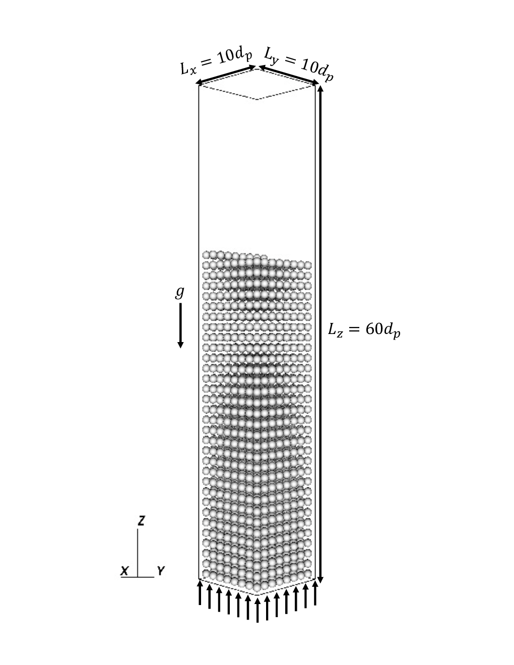
The average upflow velocity at the inlet, , is varied to investigate Reynolds number effects. A total of six simulations were conducted with m s-1, giving where . For all cases, the pressure is specified at the top boundary as , while at the bottom boundary the inflow velocity is specified and all side wall boundary conditions are periodic. Due to the absence of walls which would produce a Poiseuille velocity profile at the inlet, the inflow velocity is uniform and given by . For collision models, the minimum separation distance in the lubrication model is set to and the dry restitution coefficient . The parameters dictating rolling/sticking and sliding are used.
Figure 16 demonstrates the relationship between the normalized velocity and the time-averaged porosity . A straight line on a log-log scale indicates the results follow a power law relationship. To assess the accuracy of the simulations, we regressed the power law (equation 53) which gives and . This is in close agreement with the values of (equation 54) and (equation 55) and trends reported by other low-porosity particle-resolved simulations [6, 8].
To demonstrate the capability to simulate polydispersed particles, we increased the simulation complexity from monodispersed to bidispersed fluidization. Here, we performed a three-dimensional simulation with particles in the reactor. The particles have two uniform diameters m and and density kg m-3. The number of particles for and are and , respectively. The fluid properties are identical to the monodispersed fluidization simulations. A uniform grid spacing with was used to ensure accuracy. The square channel dimensions were identical, giving a grid with 2562561536 points. The inflow velocity was 0.35 m s-1, giving calculated based on as 70. The time-step size is calculated with both advection and diffusion Courant numbers that are defined as and , respectively. We ensure that the maximum Courant number . Figure 17 shows the time-avergaed porosity as a function of . The segregated bidispersed fluidized bed consists of three regions with the following properties, in order from the bottom to the top of the reactor: (1) monodispersed fluidization with particles of size , (2) bidispersed fluidization consisting of both particle sizes, and (3) monodispersed fluidization with particles of size . We computed the spatially-averaged porosity for the lower and upper regions as and , respectively which are approximately equivalent to the time-averaged porosity obtained for the equivalent monodispersed fluidization simulations ( and ). These results indicate that bidispersed fluidized beds essentially segregate into layers that behave like their monodispersed equivalents, as discussed extensively in a paper using the present method by Yao et al. [3].


4 Conclusion
We develop a modified particle-resolved simulation framework that combines the collocated-grid Immersed Boundary Method and colision models for polydisperse particles. An improved Immersed Boundary Method [24] is coupled with the fractional step method [34] to solve the Navier Stokes equations. The method is shown to be slightly higher than first-order accurate in space and scales well on hundreds of processors on high-performance parallel computing platforms. To enforce no-slip boundary conditions on particle surfaces, a tuning parameter, the number of outer forcing loops , was introduced and calibrated based on experiments. The accuracy of fluid-particle interactions was validated against various test cases corresponding to a single particle settling in a periodic domain with different terminal settling velocities. These cases showed that the tuning parameter . Since the Immersed Boundary Method does not resolve the fluid-particle interactions when particles are very close to or in contact with one another, collision models are implemented to simulate the interactions between particles and flow. The normal contact model we implement is based on the adaptive collision time step model proposed by Kempe and Fröhlich [27] to remove the constraint resulting from the collision time-step size which is typically much smaller than the fluid time-step size. The tangential contact model utilizes a spring-dash-pot model [16] while the lubrication model is modified based on an algebraic relationship. To ensure accurate collisions between particles, specification of the minimum separation distance between particles, , is needed. Since affects both fluid-particle and particle-particle interactions, and must be calibrated to reproduce experimental results of particle-wall interactions. The collision models are calibrated with experimental results of a single particle colliding with a wall, in which the rebound height of the particle matches the experimental rebound trajectories with tuning parameters and . Our results also show that a grid resolution of can produce results that closely match the experiments. These parameters represent a good balance between computational cost and accuracy. Finally, our collocated-grid simulation framework for polydispersed particles was used to simulate both monodispersed and bidispersed fluidized-bed expansion, demonstrating its capability in reproducing the power law relationship between superficial velocity and porosity.
Acknowledgments
This work used the Extreme Science and Engineering Discovery Environment (XSEDE), which is supported by National Science Foundation grant number ACI-1548562. Simulations were conducted with supercomputer resources under XSEDE Project CTS190063. The authors acknowledge the Texas Advanced Computing Center (TACC) at The University of Texas at Austin for providing HPC resources that have contributed to the research results reported within this paper. This work was funded by the California Energy Commission (CEC) under CEC project number EPC-16-017, the U.S. NSF Engineering Center for Reinventing of the Nation’s Urban Water Infrastructure (ReNUWIt) under Award No. 1028968, and Office of Naval Research Grant N00014-16-1-2256. Bernhard Vowinckel gratefully acknowledges the support through the German Research Foundation, (DFG) grant VO2413/2-1. This paper was prepared as a result of work sponsored in part by the California Energy Commission. It does not necessarily represent the views of the Energy Commission, its employees, or the State of California. Neither the Commission, the State of California, nor the Commission’s employees, contractors, or subcontractors makes any warranty, express or implied, or assumes any legal liability for the information in this paper; nor does any party represent that the use of this information will not infringe upon privately owned rights. This paper has not been approved or disapproved by the Commission, nor has the Commission passed upon the accuracy of the information in this paper.
References
- [1] Shin C, McCarty PL, Kim J, Bae J. Pilot-scale temperate-climate treatment of domestic wastewater with a staged anaerobic fluidized membrane bioreactor (SAF-MBR). Bioresour. Technol. 2014; 159: 95–103. doi: 10.1016/j.biortech.2014.02.060
- [2] Yao Y, Criddle CS, Fringer OB. The effects of particle clustering on hindered settling in high-concentration particle suspensions. J. Fluid Mech. 2021; 920: A40. doi: 10.1017/jfm.2021.470
- [3] Yao Y, Criddle CS, Fringer OB. Comparison of the properties of segregated layers in a bidispersed fluidized bed to those of a monodispersed fluidized bed. Phys. Rev. Fluids 2021; 6(8): 084306. doi: 10.1103/PhysRevFluids.6.084306
- [4] Fringer OB, Dawson CN, He R, Ralston DK, Zhang YJ. The future of coastal and estuarine modeling: Findings from a workshop. Ocean Model. 2019; 143: 101458. doi: 10.1016/j.ocemod.2019.101458
- [5] Richardson JF, Zaki WN. Sedimentation and Fluidisation: Part I. Trans. Inst. Chem. Eng. 1954; 32: 35–53.
- [6] Yin X, Koch DL. Hindered settling velocity and microstructure in suspensions of solid spheres with moderate Reynolds numbers. Phys. Fluids 2007; 19(9): 093302. doi: 10.1063/1.2764109
- [7] Zhang Z, Prosperetti A. A second-order method for three-dimensional particle simulation. J. Comput. Phys. 2005; 210(1): 292–324. doi: 10.1016/j.jcp.2005.04.009
- [8] Willen DP, Prosperetti A. Resolved simulations of sedimenting suspensions of spheres. Phys. Rev. Fluids 2019; 4(1): 014304. doi: 10.1103/PhysRevFluids.4.014304
- [9] Glowinski R, Pan TW, Hesla TI, Joseph DD. A distributed Lagrange multiplier/fictitious domain method for particulate flows. Int. J. Multiphase Flow 1999; 25(5): 755–794. doi: 10.1016/S0301-9322(98)00048-2
- [10] Glowinski R, Pan TW, Hesla TI, Joseph DD, Périaux J. A Fictitious Domain Approach to the Direct Numerical Simulation of Incompressible Viscous Flow past Moving Rigid Bodies: Application to Particulate Flow. J. Comput. Phys. 2001; 169(2): 363–426. doi: 10.1006/jcph.2000.6542
- [11] Ladd AJC. Hydrodynamic interactions and the viscosity of suspensions of freely moving spheres. J. Chem. Phys. 1989; 90(2): 1149–1157. doi: 10.1063/1.456170
- [12] Peskin CS. Numerical analysis of blood flow in the heart. J. Comput. Phys. 1977; 25(3): 220–252. doi: 10.1016/0021-9991(77)90100-0
- [13] Peskin CS. The immersed boundary method. Acta Numer. 2002; 11: 479–517. doi: 10.1017/S0962492902000077
- [14] Uhlmann M. An immersed boundary method with direct forcing for the simulation of particulate flows. J. Comput. Phys. 2005; 209(2): 448–476. doi: 10.1016/j.jcp.2005.03.017
- [15] Akiki G, Balachandar S. Immersed boundary method with non-uniform distribution of Lagrangian markers for a non-uniform Eulerian mesh. J. Comput. Phys. 2016; 307: 34–59. doi: 10.1016/j.jcp.2015.11.019
- [16] Biegert E, Vowinckel B, Meiburg E. A collision model for grain-resolving simulations of flows over dense, mobile, polydisperse granular sediment beds. J. Comput. Phys. 2017; 340: 105–127. doi: 10.1016/j.jcp.2017.03.035
- [17] Kim J, Kim D, Choi H. An Immersed-Boundary Finite-Volume Method for Simulations of Flow in Complex Geometries. J. Comput. Phys. 2001; 171(1): 132–150. doi: 10.1006/jcph.2001.6778
- [18] Wang Z, Fan J, Luo K. Combined multi-direct forcing and immersed boundary method for simulating flows with moving particles. Int. J. Multiphase Flow 2008; 34(3): 283–302. doi: 10.1016/j.ijmultiphaseflow.2007.10.004
- [19] Breugem WP. A second-order accurate immersed boundary method for fully resolved simulations of particle-laden flows. J. Comput. Phys. 2012; 231(13): 4469–4498. doi: 10.1016/j.jcp.2012.02.026
- [20] Apte SV, Martin M, Patankar NA. A numerical method for fully resolved simulation (FRS) of rigid particle–flow interactions in complex flows. J. Comput. Phys. 2009; 228(8): 2712–2738. doi: 10.1016/j.jcp.2008.11.034
- [21] Apte SV, Finn JR. A variable-density fictitious domain method for particulate flows with broad range of particle–fluid density ratios. J. Comput. Phys. 2013; 243: 109–129. doi: 10.1016/j.jcp.2012.12.021
- [22] Yu Z, Shao X. A direct-forcing fictitious domain method for particulate flows. J. Comput. Phys. 2007; 227(1): 292–314. doi: 10.1016/j.jcp.2007.07.027
- [23] Huang WX, Tian FB. Recent trends and progress in the immersed boundary method. Proc Inst Mech Eng Part C 2019; 233(23-24): 7617–7636. doi: 10.1177/0954406219842606
- [24] Kempe T, Fröhlich J. An improved immersed boundary method with direct forcing for the simulation of particle laden flows. J. Comput. Phys. 2012; 231(9): 3663–3684. doi: 10.1016/j.jcp.2012.01.021
- [25] Zhou K, Balachandar S. An analysis of the spatio-temporal resolution of the immersed boundary method with direct forcing. J. Comput. Phys. 2021; 424: 109862. doi: 10.1016/j.jcp.2020.109862
- [26] Yang Y, Balachandar S. A scalable parallel algorithm for direct-forcing immersed boundary method for multiphase flow simulation on spectral elements. J. Supercomput. 2021; 77(3): 2897–2927. doi: 10.1007/s11227-020-03371-2
- [27] Kempe T, Fröhlich J. Collision modelling for the interface-resolved simulation of spherical particles in viscous fluids. J. Fluid Mech. 2012; 709: 445–489. doi: 10.1017/jfm.2012.343
- [28] Yu Z, Lin Z, Shao X, Wang LP. A parallel fictitious domain method for the interface-resolved simulation of particle-laden flows and its application to the turbulent channel flow. Engineering Applications of Computational Fluid Mechanics 2016; 10(1): 160–170. doi: 10.1080/19942060.2015.1092268
- [29] Xia Y, Xiong H, Yu Z, Zhu C. Effects of the collision model in interface-resolved simulations of particle-laden turbulent channel flows. Phys. Fluids 2020; 32(10): 103303. doi: 10.1063/5.0020995
- [30] Kidanemariam AG, Uhlmann M. Interface-resolved direct numerical simulation of the erosion of a sediment bed sheared by laminar channel flow. Int. J. Multiphase Flow 2014; 67: 174–188. doi: 10.1016/j.ijmultiphaseflow.2014.08.008
- [31] Zaidi AA, Tsuji T, Tanaka T. Hindered Settling Velocity & Structure Formation during Particle Settling by Direct Numerical Simulation. Procedia Eng. 2015; 102: 1656–1666. doi: 10.1016/j.proeng.2015.01.302
- [32] Luding S. Cohesive, frictional powders: contact models for tension. Granular Matter 2008; 10(4): 235. doi: 10.1007/s10035-008-0099-x
- [33] Thornton C, Cummins SJ, Cleary PW. An investigation of the comparative behaviour of alternative contact force models during inelastic collisions. Powder Technol. 2013; 233: 30–46. doi: 10.1016/j.powtec.2012.08.012
- [34] Zang Y, Street RL, Koseff JR. A Non-staggered Grid, Fractional Step Method for Time-Dependent Incompressible Navier-Stokes Equations in Curvilinear Coordinates. J. Comput. Phys. 1994; 114(1): 18–33. doi: 10.1006/jcph.1994.1146
- [35] Lee H, Balachandar S. Drag and lift forces on a spherical particle moving on a wall in a shear flow at finite Re. J. Fluid Mech. 2010; 657: 89–125. doi: 10.1017/S0022112010001382
- [36] Lee H, Ha MY, Balachandar S. Rolling/sliding of a particle on a flat wall in a linear shear flow at finite Re. Int. J. Multiphase Flow 2011; 37(2): 108–124. doi: 10.1016/j.ijmultiphaseflow.2010.10.005
- [37] Zhang X, Gu X, Ma N. A ghost-cell immersed boundary method on preventing spurious oscillations for incompressible flows with a momentum interpolation method. Comput. Fluids 2021; 220: 104871. doi: 10.1016/j.compfluid.2021.104871
- [38] Mittal R, Dong H, Bozkurttas M, Najjar FM, Vargas A, Loebbecke vA. A VERSATILE SHARP INTERFACE IMMERSED BOUNDARY METHOD FOR INCOMPRESSIBLE FLOWS WITH COMPLEX BOUNDARIES. J. Comput. Phys. 2008; 227(10): 4825–4852. doi: 10.1016/j.jcp.2008.01.028
- [39] Tseng YH, Ferziger JH. A ghost-cell immersed boundary method for flow in complex geometry. J. Comput. Phys. 2003; 192(2): 593–623. doi: 10.1016/j.jcp.2003.07.024
- [40] Gilmanov A, Sotiropoulos F. A hybrid Cartesian/immersed boundary method for simulating flows with 3D, geometrically complex, moving bodies. J. Comput. Phys. 2005; 207(2): 457–492. doi: 10.1016/j.jcp.2005.01.020
- [41] Fadlun EA, Verzicco R, Orlandi P, Mohd-Yusof J. Combined Immersed-Boundary Finite-Difference Methods for Three-Dimensional Complex Flow Simulations. J. Comput. Phys. 2000; 161(1): 35–60. doi: 10.1006/jcph.2000.6484
- [42] Roma AM, Peskin CS, Berger MJ. An Adaptive Version of the Immersed Boundary Method. J. Comput. Phys. 1999; 153(2): 509–534. doi: 10.1006/jcph.1999.6293
- [43] Rai M, Moin P. Direct simulations of turbulent flow using finite-difference schemes. J. Comput. Phys. 1991; 96(1): 15–53. doi: 10.1016/0021-9991(91)90264-l
- [44] Uhlmann M. First experiments with the simulation of particulate flows. Centro de Investigaciones Energeticas Medioambientales y Tecnologicas (CIEMAT) 2003.
- [45] Uhlmann M. New results on the simulation of particulate flows. Centro de Investigaciones Energeticas Medioambientales y Tecnologicas (CIEMAT) 2004.
- [46] Rhie CM, Chow WL. Numerical study of the turbulent flow past an airfoil with trailing edge separation. AIAA Journal 1983; 21(11): 1525–1532. doi: 10.2514/3.8284
- [47] Ferziger JH, Perić M, Street RL. Computational Methods for Fluid Dynamics. Springer . 2019.
- [48] Luo K, Wang Z, Fan J, Cen K. Full-scale solutions to particle-laden flows: Multidirect forcing and immersed boundary method. Phys. Rev. E Stat. Nonlin. Soft Matter Phys. 2007; 76(6 Pt 2): 066709. doi: 10.1103/PhysRevE.76.066709
- [49] Biegert EK. Eroding Uncertainty: Towards Understanding Flows Interacting with Mobile Sediment Beds Using Grain-Resolving Simulations. PhD thesis. UC Santa Barbara, 2018.
- [50] Höfler K, Schwarzer S. Navier-Stokes simulation with constraint forces: Finite-difference method for particle-laden flows and complex geometries. Phys. Rev. E 2000; 61(6 Pt B): 7146–7160. doi: 10.1103/physreve.61.7146
- [51] Cox RG, Brenner H. The slow motion of a sphere through a viscous fluid towards a plane surface—II Small gap widths, including inertial effects. Chem. Eng. Sci. 1967; 22(12): 1753–1777. doi: 10.1016/0009-2509(67)80208-2
- [52] Ray S, Kempe T, Fröhlich J. Efficient modelling of particle collisions using a non-linear viscoelastic contact force. Int. J. Multiphase Flow 2015; 76: 101–110. doi: 10.1016/j.ijmultiphaseflow.2015.06.006
- [53] Thornton C, Cummins SJ, Cleary PW. An investigation of the comparative behaviour of alternative contact force models during elastic collisions. Powder Technol. 2011; 210(3): 189–197. doi: 10.1016/j.powtec.2011.01.013
- [54] Costa P, Boersma BJ, Westerweel J, Breugem WP. Collision model for fully resolved simulations of flows laden with finite-size particles. Phys. Rev. E Stat. Nonlin. Soft Matter Phys. 2015; 92(5): 053012. doi: 10.1103/PhysRevE.92.053012
- [55] Cate tA, Nieuwstad CH, Derksen JJ, Akker V. dHEA. Particle imaging velocimetry experiments and lattice-Boltzmann simulations on a single sphere settling under gravity. Phys. Fluids 2002; 14(11): 4012–4025. doi: 10.1063/1.1512918
- [56] Mordant N, Pinton JF. Velocity measurement of a settling sphere. Eur. Phys. J. B 2000; 18(2): 343–352. doi: 10.1007/PL00011074
- [57] Armfield S, Street R. An analysis and comparison of the time accuracy of fractional-step methods for the Navier-Stokes equations on staggered grids. Int. J. Numer. Methods Fluids 2002; 38(3): 255–282. doi: 10.1002/fld.217
- [58] Gondret P, Lance M, Petit L. Bouncing motion of spherical particles in fluids. Phys. Fluids 2002; 14(2): 643–652. doi: 10.1063/1.1427920
- [59] Falgout RD. An introduction to algebraic multigrid. Computing in Science Engineering 2006; 8(6): 24–33. doi: 10.1109/MCSE.2006.105
- [60] Towns J, Cockerill T, Dahan M, et al. XSEDE: Accelerating Scientific Discovery. Computing in Science Engineering 2014; 16(5): 62–74. doi: 10.1109/MCSE.2014.80
- [61] Yao Y, Criddle CS, Fringer OB. Competing flow and collision effects in a monodispersed liquid–solid fluidized bed at a moderate Archimedes number. J. Fluid Mech. 2021; 927: A28. doi: 10.1017/jfm.2021.780
- [62] Garside J, Al-Dibouni MR. Velocity-Voidage Relationships for Fluidization and Sedimentation in Solid-Liquid Systems. Ind. Eng. Chem. Proc. Des. Dev. 1977; 16(2): 206–214. doi: 10.1021/i260062a008