跳到论文正文
W Papers独立论文阅读器 arXiv:2109.03885 论文正文 计算阅读时间 · 0%
引用这篇论文根据当前论文元数据生成,正式投稿前建议核对。


License: arXiv.org perpetual non-exclusive license
arXiv:2109.03885v1 [gr-qc] 08 Sep 2021

A new shape function and some specific wormhole solutions in braneworld scenario

Bikram Ghosh Note: bikramghosh13@gmail.com Affiliation: Department of Mathematics, Ramakrishna Mission Vidyamandira, Howrah-711202, West Bengal, India    Saugata Mitra Note: saugatamitra20@gmail.com Affiliation: Department of Mathematics, Ramakrishna Mission Vidyamandira, Howrah-711202, West Bengal, India
Abstract

Considering a energy density of the form ρ=q​(rr0)−n\rho=q\left({\frac{r}{r_{0}}}\right)^{-n}( where qq is an arbitrary positive constant with dimension of energy density and n>0n>0), a shape function is obtained by using field equations of braneworld gravity theory in this paper. Under isotropic scenario wormhole solutions are obtained considering six different redshift functions along with the obtained new shape function. For anisotropic case wormhole solutions are obtained under the consideration of five different shape functions along with the redshift function ϕ=β​l​n​(rr0)\phi=\beta ln(\frac{r}{r_{0}}), where β\beta is an arbitrary constant. In each case all the energy conditions are examined and it is found that for some cases all energy conditions are satisfied in the vicinity of the wormhole throat and for the rest cases all energy conditions are satisfied except strong energy condition.

I Introduction

In the context of string theoryb1–b2, the brane (i.e., the observed four dimensional world) is considered as a domain wall in the five dimensional space-time. Geometrically, braneb3–b4 is considered as a four dimensional hypersurface embedded in a five dimensional bulk (for a review seeb5–b6). In Randall-Sundrum type-IIb4 brane model, our universe (i.e., 3 brane) is embedded in a five-dimensional bulk with extra dimension extending to infinity in either side of the brane. In this model all standard model fields are confined to the brane while gravity can propagate in the surrounding bulk. Starting from the five-dimensional Einstein field equations in the bulk and using Gauss and Codazzi equations Shiromizu et al.b7 derived the modified four-dimensional Einstein equations on the brane. The above modified Einstein field equations has two extra terms in the r.h.s– one correction term is quadratic in the energy-momentum tensor on the brane and is termed as local bulk effect while the non-local bulk effect is the electric part of the 5​D5D Weyl tensor. Hence the effective Einstein equations on the brane can be written as r24–r15

Gμ​ν=−Λ​gμ​ν+k2​(Tμ​ν+6λ​Pμ​ν)−ξμ​ν,G_{\mu\nu}=-\Lambda g_{\mu\nu}+k^{2}(T_{\mu\nu}+\frac{6}{\lambda}P_{\mu\nu})-\xi_{\mu\nu}, (1)

where the terms on the r.h.s of the above modified Einstein equation are the followings: Λ=12​(Λ5+k2​λ)\Lambda=\frac{1}{2}(\Lambda_{5}+k^{2}\lambda), k2=λ​k526k^{2}=\frac{\lambda k_{5}^{2}}{6} ,

Pμ​ν=18​[23​T​Tμ​ν−2​Tμ​ψ​Tνψ+gμ​ν​{Tψ​τ​Tψ​τ−13​T2}],P_{\mu\nu}=\frac{1}{8}\bigg[\frac{2}{3}TT_{\mu\nu}-2T_{\mu\psi}T_{\nu}^{\psi}+g_{\mu\nu}\biggl\{T_{\psi\tau}T^{\psi\tau}-\frac{1}{3}T^{2}\biggr\}\bigg], (2)

and ξμ​ν=δμA​δνC​WA​B​C​D​ηB​ηD\xi_{\mu\nu}=\delta_{\mu}^{A}\delta_{\nu}^{C}W_{ABCD}\eta^{B}\eta^{D}. Here k2k^{2} and k52k_{5}^{2} are gravitational coupling constants on brane and bulk respectively, Λ\Lambda and Λ5\Lambda_{5} are the cosmological constants on the brane and bulk respectively, λ\lambda is the brane tension, Tμ​νT_{\mu\nu} is the energy momentum tensor for the matter on the brane (with T=Tμ​ν​gμ​νT=T_{\mu\nu}g^{\mu\nu} is the trace of the energy momentum tensor), Pμ​νP_{\mu\nu} is the local correction term, ξμ​ν\xi_{\mu\nu} is the (trace less i.e., ξμμ=0\xi^{\mu}_{\mu}=0) non-local bulk effect(which is the projection of the 5​D5D dimensional Weyl tensor WA​B​C​DW_{ABCD}) and ηa\eta^{a} is the unit normal to the brane.

Wormhole is a hypothetical geometric structure in space-time r1–r3. It can be considered as tunnels in the space-time topology. In fact this topological structure connects two distant parts of a single universe or even of different universes. The wormhole geometry is characterized by the solution of the Einstein equations with exotic matter (that violates the null energy condition) at least in the vicinity of the wormhole throatr6–r8. In spherically symmetric space-time, traversable wormhole is most interesting and physically viable and such type of wormhole was initiated by the pioneering work of Morris and Throner4–r5. The restriction in the geometry of the space-time due to the traversability nature of the wormhole is that the redshift function should not have any horizon or it is desirable to have a given asymptotic form for both the redshift and shape function. Usually, in the literature wormhole solutions are constructed knowing a priori the desired form of the redshift function and the shape function and Einstein field equations determine the matter part for the wormhole geometry.

Braneworld gravityr12 is an important model of the universe in modified gravity theory and obtainig wormhole solutions in this gravity is attracted to researchersr13-r17, where wormhole solutions are obtained under different considerations. In r24, wormhole solutions are obtained by equating RR with zero. Inflating wormhole solutions are obtained inr18. In the literature there are many examples of wormhole solutions where null energy condition is satisfiedr20-r23.

In this paper, a new shape function is found by considering a particular form of energy density and the main motivation is to examine whether all energy conditions are satisfied or not in the wormhole solutions which are obtained by considering isotropic fluid and using the new shape function along with the following redshift functions: ϕ⁡(r)=constant\phi(r)=\text{constant}; ϕ⁡(r)=β​l​n​(rr0)\phi(r)=\beta ln\left(\frac{r}{r_{0}}\right), β\beta is a arbitrary constant; ϕ⁡(r)=1r\phi(r)=\frac{1}{r}; ϕ⁡(r)=l​n​γ2+r2r\phi(r)=ln\frac{\sqrt{\gamma^{2}+r^{2}}}{r}, γ\gamma is a arbitrary constant; ϕ⁡(r)=e−r0r\phi(r)=e^{-\frac{r_{0}}{r}}; ϕ⁡(r)=e−r0r−r02r2\phi(r)=e^{-\frac{r_{0}}{r}-\frac{r_{0}^{2}}{r^{2}}}r25-r26. Other wormhole solutions for anisotropic fluid using shape functions: b⁡(r)=r0nrn−1b(r)=\frac{r_{0}^{n}}{r^{n-1}},(n>0n>0); b⁡(r)=r1+l​n​(1+r−r0)b(r)=\frac{r}{1+ln(1+r-r_{0})}, (0<r0<10<r_{0}<1); b⁡(r)=r1+r−r0,(0<r0<1)b(r)=\frac{r}{1+r-r_{0}},\penalty\ (0<r_{0}<1); b⁡(r)=r0​{1+γ2​(1−r0r)}b(r)=r_{0}\biggl\{1+\gamma^{2}\biggl(1-\frac{r_{0}}{r}\biggr)\biggr\}, (γ2∈(0,1)\gamma^{2}\in(0,1))r19 and b⁡(r)=r​e2​σδ​(rδ−r0δ)b(r)=re^{\frac{2\sigma}{\delta}(r^{\delta}-r_{0}^{\delta})} (σ<0\sigma<0 and δ>0\delta>0)r25-r26 and redshift function ϕ⁡(r)\phi(r)=β​l​n​(rr0)\beta ln(\frac{r}{r_{0}}) are obtained and energy conditions are also examined in this cases.
The paper is arranged as follows : in section II, the necessary field equations on Brane-world are discussed. In section III energy conditions of wormholes are mentioned. A wormhole shape function is obtained in section IV. Energy conditions are examined in section V for isotropic fluid. For anisotropic fluid wormhole solutions are obtained, energy conditions are examined in section VI. Lastly, we discuss our overall observations in section VII.

II Field equations on the brane

The space-time metric representing a spherically symmetric and static wormhole is given by r4

d​s2=−e2​ϕ​(r)​d​t2+d​r21−b⁡(r)r+r2​(d​θ2+sin2⁡θ​d​ϕ2),ds^{2}=-e^{2\phi(r)}dt^{2}+\frac{dr^{2}}{1-\frac{b(r)}{r}}+r^{2}(d\theta^{2}+{\sin^{2}\theta}d\phi^{2}), (3)

where ϕ⁡(r)\phi(r) and b⁡(r)b(r) are arbitrary function of radial co-ordinate `​r`r’, termed as redshift function and shape function respectively. The former is related to gravitational redshift, while the latter determines the shape of the wormhole. The event horizon should be absent for traversable wormhole, for which we require e2​ϕ​(r)≠0e^{2\phi(r)}\neq 0 i.e., ϕ⁡(r)\phi(r) should be finite everywhere. Now for the existence of wormhole, the shape function b⁡(r)b(r) is restricted as follows (i)(i) b⁡(r0)=r0b(r_{0})=r_{0} (r0r_{0} is the location of the throat), (i​i)(ii) b⁡(r)r<1\frac{b(r)}{r}<1 for r>r0r>r_{0}, (i​i​i)(iii) b⁡(r)r→0\frac{b(r)}{r}\rightarrow 0 and ϕ⁡(r)→ϕ0\phi(r)\rightarrow\phi_{0}(constant) as r→∞r\rightarrow\infty (asymptotically flatness propertyr4-r5), (i​v)(iv) b−b′​r2​b2>0\frac{b-b^{\prime}r}{2b^{2}}>0 is the condition for flare-outr4.

The field equation on the brane can take the form

Gμ​ν=8​π​Tμ​νeff,G_{\mu\nu}=8\pi T_{\mu\nu}^{\text{eff}}, (4)

with the total effective stress-energy tensor,

Tμ​νeff=Tμ​ν−18​π​ξμ​ν+6λ​Pμ​ν​ with ​k2=8​π.T_{\mu\nu}^{\text{eff}}=T_{\mu\nu}-\frac{1}{8\pi}\xi_{\mu\nu}+\frac{6}{\lambda}P_{\mu\nu}\text{\penalty\ \penalty\ \penalty\ \penalty\ with\penalty\ \penalty\ }k^{2}=8\pi. (5)

For simplicity we have considered Λ=0\Lambda=0 on the brane and hence Einstein tensor components (with respect to an orthonormal reference frame) for the metric (3) can be written as

Gt​t\displaystyle G_{tt} =\displaystyle= b′r2,\displaystyle\frac{b^{\prime}}{r^{2}}, (6)
Gr​r\displaystyle G_{rr} =\displaystyle= 2​(1−1r)​ϕ′r−br3,\displaystyle 2\biggl(1-\frac{1}{r}\biggr)\frac{\phi^{\prime}}{r}-\frac{b}{r^{3}}, (7)
Gθ​θ=Gϕ​ϕ\displaystyle G_{\theta\theta}=G_{\phi\phi} =\displaystyle= (1−br)​[ϕ′′+(ϕ′)2+ϕ′r−b′​r−b2​r2​(r−b)−b′​r−b2​r​(r−b)​ϕ′],\displaystyle\biggl(1-\frac{b}{r}\biggr)\biggl[\phi^{\prime\prime}+(\phi^{\prime})^{2}+\frac{\phi^{\prime}}{r}-\frac{b^{\prime}r-b}{2r^{2}(r-b)}-\frac{b^{\prime}r-b}{2r(r-b)}\phi^{\prime}\biggr], (8)

where the prime denotes the derivative with respect to the radial coordinate `​r`r’. From (1), the traceless property of the projected 5-dimensional Weyl-tensor givesr15

R=−k2​{T+32​λ​(Tψ​τ​Tψ​τ−13​T2)}R=-k^{2}\biggl\{T+\frac{3}{2\lambda}\left(T_{\psi\tau}T^{\psi\tau}-\frac{1}{3}T^{2}\right)\biggr\} (9)

i.e.,

R=−k2​[(−ρ+pr+2​pt)+32​λ​{ρ2+pr2+2​pt2−13​(−ρ+pr+2​pt)2}].R=-k^{2}\bigg[(-\rho+p_{r}+2p_{t})+\frac{3}{2\lambda}\biggl\{\rho^{2}+p_{r}^{2}+2p_{t}^{2}-\frac{1}{3}\bigg(-\rho+p_{r}+2p_{t}\bigg)^{2}\biggr\}\bigg]. (10)

Also from the definition of Ricci scalar (RR)r30 we get,

R=−2​(1−br)​[ϕ′′+(ϕ′)2−b′r⁡(r−b)−b′​r+3​b−4​r2​r​(r−b)​ϕ′]R=-2\biggl(1-\frac{b}{r}\biggr)\biggl[\phi^{\prime\prime}+(\phi^{\prime})^{2}-\frac{b^{\prime}}{r(r-b)}-\frac{b^{\prime}r+3b-4r}{2r(r-b)}\phi^{\prime}\biggr] (11)

and the result becomes R|r=r0=2​b0′r02+(b0′−1)​ϕ0′r02R|_{r=r_{0}}=\frac{2b_{0}^{\prime}}{r_{0}^{2}}+\frac{(b_{0}^{\prime}-1)\phi_{0}^{\prime}}{r_{0}^{2}} at the throat.

III Energy conditions

The null energy condition (NEC), weak energy condition (WEC), strong energy condition (SEC) and dominant energy conditions (DEC) are considered main energy conditions in the background of brane-world gravity. These will be investigated by the following inequalities depending on energy momentum tensor characterize the energy conditions as followsr29-r30:

(I)\displaystyle(I) NEC:ρ+pr≥0,ρ+pt≥0\displaystyle\text{NEC}:\rho+p_{r}\geq 0,\rho+p_{t}\geq 0 (12)
(I​I)\displaystyle(II) WEC:ρ≥0,ρ+pr≥0,ρ+pt≥0\displaystyle\text{WEC}:\rho\geq 0,\rho+p_{r}\geq 0,\rho+p_{t}\geq 0 (13)
(I​I​I)\displaystyle(III) SEC:ρ+pr≥0,ρ+pt≥0,ρ+pr+2​pt≥0\displaystyle\text{SEC}:\rho+p_{r}\geq 0,\rho+p_{t}\geq 0,\rho+p_{r}+2p_{t}\geq 0 (14)
(I​V)\displaystyle(IV) DEC:ρ≥0,ρ−|pr|≥0,ρ−|pt|≥0.\displaystyle\text{DEC}:\rho\geq 0,\rho-|p_{r}|\geq 0,\rho-|p_{t}|\geq 0. (15)

For the isotropic fluid with radial pressure pp, the above set becomes:

(I)\displaystyle(I) NEC:ρ+p≥0\displaystyle\text{NEC}:\rho+p\geq 0 (16)
(I​I)\displaystyle(II) WEC:ρ≥0,ρ+p≥0\displaystyle\text{WEC}:\rho\geq 0,\rho+p\geq 0 (17)
(I​I​I)\displaystyle(III) SEC:ρ+p≥0,ρ+3​p≥0\displaystyle\text{SEC}:\rho+p\geq 0,\rho+3p\geq 0 (18)
(I​V)\displaystyle(IV) DEC:ρ≥0,ρ−|p|≥0.\displaystyle\text{DEC}:\rho\geq 0,\rho-|p|\geq 0. (19)

IV Obtaining Shape function

For an isotropic fluid on the brane, the energy momentum tensor can be written as Tνμ=T^{\mu}_{\nu}=diag(−ρ,p,p,p)(-\rho,p,p,p)r15 where ρ\rho is energy density, pp is isotropic radial pressure of the fluid. As a result, the nonlocal bulk effects contribute in the form an effective anisotropic fluid as

ξνμ=diag​[−ϵ⁡(r),σr​(r),σt​(r),σt​(r)],\xi^{\mu}_{\nu}=\text{diag}[-\epsilon(r),\sigma_{r}(r),\sigma_{t}(r),\sigma_{t}(r)], (20)

and the traceless property of ξμ​ν\xi_{\mu\nu} gives

−ϵ+σr+2​σt=0.-\epsilon+\sigma_{r}+2\sigma_{t}=0. (21)

Now using equations (4) and (5) we get the effective field equations from (6)–(8) asr19:

b′r2\displaystyle\frac{b^{\prime}}{r^{2}} =\displaystyle= ρ⁡(1+ρ2​λ)−ϵ8​π,\displaystyle\rho(1+\frac{\rho}{2\lambda})-\frac{\epsilon}{8\pi}, (22)
2r​(1−br)​ϕ′−br3\displaystyle\frac{2}{r}\left(1-\frac{b}{r}\right)\phi^{\prime}-\frac{b}{r^{3}} =\displaystyle= p⁡(1+ρλ)+ρ22​λ−σr8​π,\displaystyle p(1+\frac{\rho}{\lambda})+\frac{\rho^{2}}{2\lambda}-\frac{\sigma_{r}}{8\pi}, (23)
(1−br)​[ϕ′′+ϕ′​(ϕ′+1r)]−b′​r−b2​r2​(ϕ′+1r)\displaystyle\left(1-\frac{b}{r}\right)\left[\phi^{\prime\prime}+\phi^{\prime}(\phi^{\prime}+\frac{1}{r})\right]-\frac{b^{\prime}r-b}{2r^{2}}(\phi^{\prime}+\frac{1}{r}) =\displaystyle= p⁡(1+ρλ)+ρ22​λ−σt8​π.\displaystyle p(1+\frac{\rho}{\lambda})+\frac{\rho^{2}}{2\lambda}-\frac{\sigma_{t}}{8\pi}. (24)

It is seen that in many wormhole theory literature the energy density takes the form ρ=k​r−s\rho=kr^{-s} where kk is a arbitrary positive constant, s=1.5s=1.5 in r30 and s=1.75s=1.75 in r31 . So let us take the form ρ=q​(rr0)−n\rho=q\left({\frac{r}{r_{0}}}\right)^{-n} for n>0n>0(where qq will take care about the dimension of energy density) and try to find shape function in this scenario.

Let us consider ϵ=0\epsilon=0. Then for the above energy density form ρ=q​(rr0)−n\rho=q\left({\frac{r}{r_{0}}}\right)^{-n} for n>0n>0, the equation (22)(\ref{eq12}) gives

b′\displaystyle b^{\prime} =\displaystyle= q​r0n​r2−n+q2​r02​n2​λ​r2−2​n.\displaystyle qr_{0}^{n}r^{2-n}+\frac{q^{2}r_{0}^{2n}}{2\lambda}r^{2-2n}. (25)
∴b\displaystyle\therefore\penalty\ b =\displaystyle= q​r0n3−n​r3−n+q2​r02​n2​(3−2​n)​λ​r3−2​n+A⁡(where A is an arbitrary constant).\displaystyle\frac{qr_{0}^{n}}{3-n}r^{3-n}+\frac{q^{2}r_{0}^{2n}}{2(3-2n)\lambda}r^{3-2n}+A\penalty\ (\text{where $A$ is an arbitrary constant}). (26)

To be a shape function bb must obey the following properties:

b⁡(r0)\displaystyle b(r_{0}) =\displaystyle= r0,\displaystyle r_{0}, (27)
br\displaystyle\frac{b}{r} ≤\displaystyle\leq 1,\displaystyle 1, (28)
b−b′​rb2\displaystyle\frac{b-b^{\prime}r}{b^{2}} >\displaystyle> 0.\displaystyle 0. (29)

Using (27)(\ref{p1}), equation (26)(\ref{e1}) reduces to

b⁡(r)=q​r0n3−n​r3−n+q2​r02​n2​(3−2​n)​λ​r3−2​n+r0−q​r033−n−q2​r032​(3−2​n)​λ.\displaystyle b(r)=\frac{qr_{0}^{n}}{3-n}r^{3-n}+\frac{q^{2}r_{0}^{2n}}{2(3-2n)\lambda}r^{3-2n}+r_{0}-\frac{qr_{0}^{3}}{3-n}-\frac{q^{2}r_{0}^{3}}{2(3-2n)\lambda}. (30)
Refer to caption

1(A)

Refer to caption

1(B)

Figure 1: Behavior of b⁡(r)r\frac{b(r)}{r}(1(A)) and b−b′​rb2\frac{b-b^{\prime}r}{b^{2}} (1(B)) with radial co-ordinate ‘rr’ and parameter nn have been plotted for obtained shape function(30) when 1≤n≤101\leq n\leq 10 and rr ranges from r0r_{0} to 10, λ=104\lambda=10^{4}, q=1q=1 and r0=1r_{0}=1.
Refer to caption

2(A)

Refer to caption

2(B)

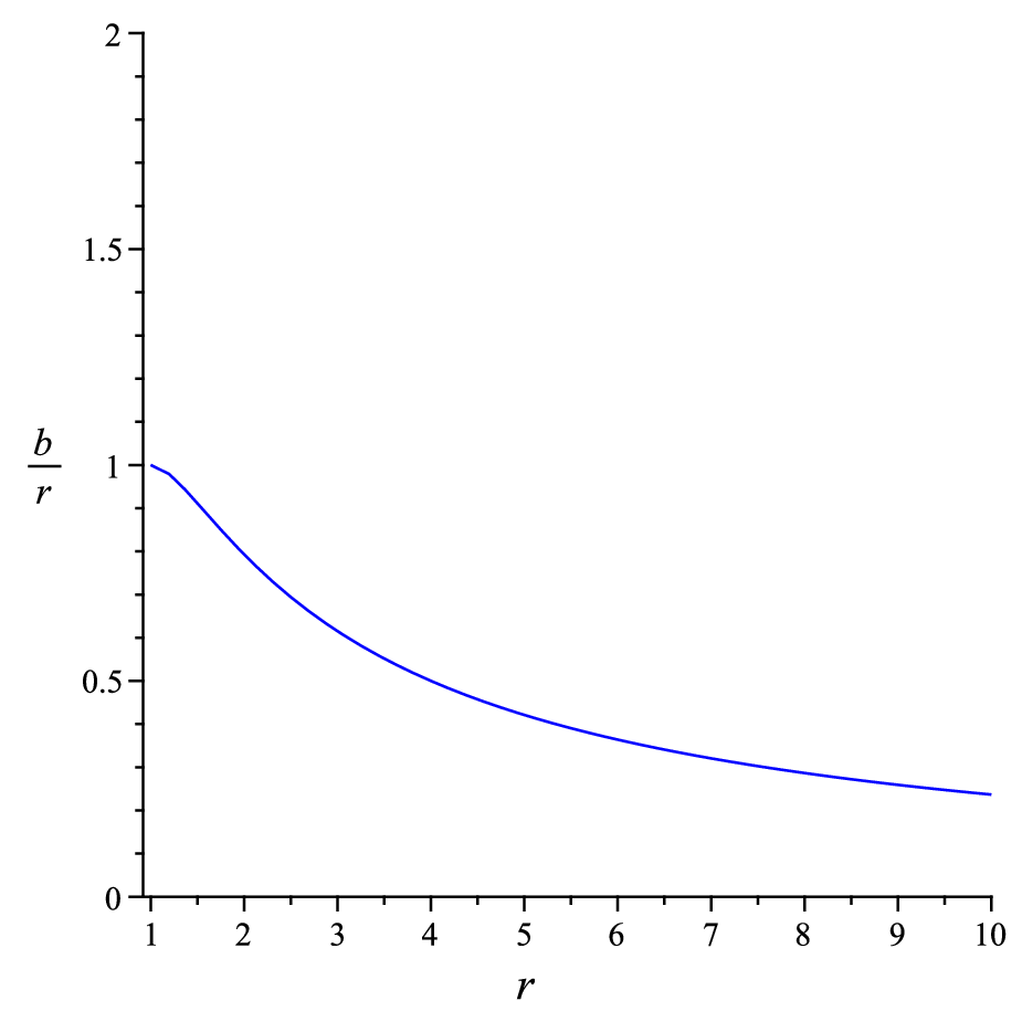
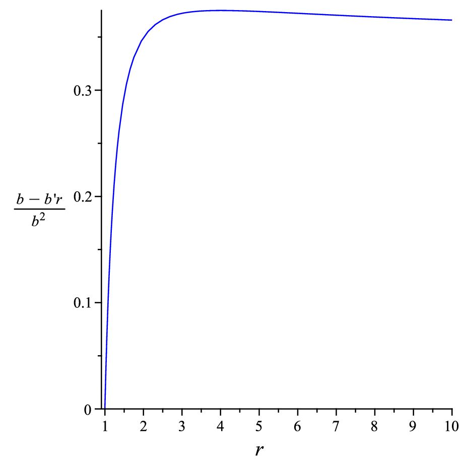
Figure 2: Behavior of b⁡(r)r\frac{b(r)}{r}(2(A)) and b−b′​rb2\frac{b-b^{\prime}r}{b^{2}} (2(B)) have been plotted for obtained shape function(30) against rr when n=3.5n=3.5, λ=104\lambda=10^{4},q=1q=1 and r0=1r_{0}=1.

The figure(1) shows that b⁡(r)b(r) is satisfying the other require conditions to be a shape function of a wormhole for n∈(3,10)n\in(3,10) (a particular scenario is shown in figure2).

V Validation of energy condition of wormhole solutions corresponds to obtained shape function for isotropic fluid

Now by equation (22)(\ref{eq12}) expression of bb (30)(\ref{b}) is obtained considering ρ=q​(rr0)−n\rho=q\left({\frac{r}{r_{0}}}\right)^{-n} for n>0n>0. Also equation (22)(\ref{eq12}) can be written as

b′=ρ2​r22​λ+ρ​r2with​b​(r0)=r0.b^{\prime}=\frac{\rho^{2}r^{2}}{2\lambda}+\rho r^{2}\penalty\ \penalty\ \text{with}\penalty\ b(r_{0})=r_{0}. (31)

The above equation(31) gives a unique solution for b⁡(r)b(r) in a neighbourhood of r0r_{0}. So if we take ϵ=0\epsilon=0, then we will get the same ρ\rho for this shape function b⁡(r)b(r). For ϵ=0\epsilon=0, equation (21) gives

σr=−2​σt.\sigma_{r}=-2\sigma_{t}. (32)

Using equation (32)(\ref{r}), equation (23)(\ref{eq13.2}) and (24)(\ref{eq14}) reduce to the form

A1​p−2​B1​σt\displaystyle A_{1}p-2B_{1}\sigma_{t} =\displaystyle= C1,\displaystyle C_{1}, (33)
A1​p+B1​σt\displaystyle A_{1}p+B_{1}\sigma_{t} =\displaystyle= C2;\displaystyle C_{2}; (34)
where​A1\displaystyle\text{where}\penalty\ A_{1} =\displaystyle= 1+ρλ;B1=−18​π;\displaystyle 1+\frac{\rho}{\lambda};\penalty\ B_{1}=\frac{-1}{8\pi};
C1\displaystyle C_{1} =\displaystyle= 2r​(1−br)​ϕ′−br3−ρ22​λ;\displaystyle\frac{2}{r}\left(1-\frac{b}{r}\right)\phi^{\prime}-\frac{b}{r^{3}}-\frac{\rho^{2}}{2\lambda};
C2\displaystyle C_{2} =\displaystyle= (1−br)​[ϕ′′+ϕ′​(ϕ′+1r)]−b′​r−b2​r2​(ϕ′+1r)−ρ22​λ.\displaystyle\left(1-\frac{b}{r}\right)\left[\phi^{\prime\prime}+\phi^{\prime}(\phi^{\prime}+\frac{1}{r})\right]-\frac{b^{\prime}r-b}{2r^{2}}(\phi^{\prime}+\frac{1}{r})-\frac{\rho^{2}}{2\lambda}.

Solving the above set of equations (33) and (34) we get,

p\displaystyle p =\displaystyle= 2​C2+C13​A1;\displaystyle\frac{2C_{2}+C_{1}}{3A_{1}}; (35)
σt\displaystyle\sigma_{t} =\displaystyle= C2−C13​B1.\displaystyle\frac{C_{2}-C_{1}}{3B_{1}}. (36)

The shape function(30) is obtained from the field equation (22) which is independent of redshift function. Now choosing different redshift functions (which are mentioned in section-I ), the validation of energy conditions are examined and they are shown in the figures (3)–(9).

Refer to caption
Figure 3: Variation of energy density (ρ\rho) with radial co-ordinate rr and parameter nn for the numerical values λ=104\lambda=10^{4}, q=1q=1 and r0=1r_{0}=1.
Refer to caption

4(A)

Refer to caption

4(B)

Refer to caption

4(C)

Figure 4: Variation of ρ+p\rho+p (4(A)), ρ+3​p\rho+3p (4(B)), pp (4(C)) with radial co-ordinate rr and parameter nn, have been plotted for obtained shape function(30) with redshift function ϕ⁡(r)=constant\phi(r)=\text{constant} when λ=104\lambda=10^{4}, q=1q=1 and r0=1r_{0}=1.
Refer to caption

5(A)

Refer to caption

5(B)

Refer to caption

5(C)

Figure 5: Variation of ρ+p\rho+p (5(A)), ρ+3​p\rho+3p (5(B)), ρ−|p|\rho-|p| (5(C)) with radial co-ordinate rr and parameter nn, have been plotted for obtained shape function(30) with redshift function ϕ⁡(r)=β​l​n​(rr0)\phi(r)=\beta ln\left(\frac{r}{r_{0}}\right) when λ=104\lambda=10^{4}, β=0.5\beta=0.5, q=1q=1 and r0=1r_{0}=1.
Refer to caption

6(A)

Refer to caption

6(B)

Refer to caption

6(C)

Figure 6: Variation of ρ+p\rho+p (6(A)), ρ+3​p\rho+3p (6(B)), pp (6(C)) with radial co-ordinate rr and parameter nn, have been plotted for obtained shape function(30) with redshift function ϕ⁡(r)=1r\phi(r)=\frac{1}{r} when λ=104\lambda=10^{4}, q=1q=1 and r0=1r_{0}=1.
Refer to caption

7(A)

Refer to caption

7(B)

Refer to caption

7(C)

Figure 7: Variation of ρ+p\rho+p (7(A)), ρ+3​p\rho+3p (7(B)), pp (7(C)) with radial co-ordinate rr and parameter nn, have been plotted for obtained shape function(30) with redshift function ϕ⁡(r)=l​n​γ2+r2r\phi(r)=ln\frac{\sqrt{\gamma^{2}+r^{2}}}{r} when λ=104\lambda=10^{4}, γ=1\gamma=1, q=1q=1 and r0=1r_{0}=1.
Refer to caption

8(A)

Refer to caption

8(B)

Refer to caption

8(C)

Figure 8: Variation of ρ+p\rho+p (8(A)), ρ+3​p\rho+3p (8(B)), ρ−|p|\rho-|p| (8(C)) with radial co-ordinate rr and parameter nn, have been plotted for obtained shape function(30) with redshift function ϕ⁡(r)=e−r0r\phi(r)=e^{-\frac{r_{0}}{r}} when λ=104\lambda=10^{4}, q=1q=1 and r0=1r_{0}=1.
Refer to caption

9(A)

Refer to caption

9(B)

Refer to caption

9(C)

Figure 9: Variation of ρ+p\rho+p (9(A)), ρ+3​p\rho+3p (9(B)), ρ−|p|\rho-|p| (9(C)) with radial co-ordinate rr and parameter nn, have been plotted for obtained shape function(30) with redshift function ϕ⁡(r)=e−r0r−r02r2\phi(r)=e^{-\frac{r_{0}}{r}-\frac{r_{0}^{2}}{r^{2}}} when λ=104\lambda=10^{4}, q=1q=1 and r0=1r_{0}=1.

VI Wormhole solutions from field equations for anisotropic fluid

We assume the relation pr=α​ptp_{r}=\alpha p_{t} (α≠1\alpha\neq 1) and consider a equation of state pt=ω​ρp_{t}=\omega\rho i.e., pr=α​ω​ρp_{r}=\alpha\omega\rho. Now we will find the wormhole solution from the above field equations (6)-(8). Using above equation of state in (10) we obtain ,

R=−k2​[(−1+α​ω+2​ω)​ρ+ρ2λ​(1+α2​ω2+ω2+α​ω+2​ω−2​α​ω2)]R=-k^{2}\biggl[(-1+\alpha\omega+2\omega)\rho+\frac{\rho^{2}}{\lambda}(1+\alpha^{2}\omega^{2}+\omega^{2}+\alpha\omega+2\omega-2\alpha\omega^{2})\biggr] (37)

i.e.,

1+α2​ω2+ω2+α​ω+2​ω−2​α​ω2λ​ρ2+(−1+α​ω+2​ω)​ρ+18​π​R=0.\frac{1+\alpha^{2}\omega^{2}+\omega^{2}+\alpha\omega+2\omega-2\alpha\omega^{2}}{\lambda}\rho^{2}+(-1+\alpha\omega+2\omega)\rho+\frac{1}{8\pi}R=0. (38)

After solving the equation(38), we get

ρ⁡(R)=−B±B2−4​A​C2​A,where​{A=1+α2​ω2+ω2+α​ω+2​ω−2​α​ω2λB=(−1+α​ω+2​ω)C=18​π​R.\rho(R)=\frac{-B\pm\sqrt{B^{2}-4AC}}{2A},\penalty\ \penalty\ \penalty\ {\text{where}}\begin{cases}A=\frac{1+\alpha^{2}\omega^{2}+\omega^{2}+\alpha\omega+2\omega-2\alpha\omega^{2}}{\lambda}\\ B=(-1+\alpha\omega+2\omega)\\ C=\frac{1}{8\pi}R\end{cases}. (39)

Consequently we have prp_{r} and ptp_{t}(in terms of ρ\rho). Thus from the value of RR, the expression of ρ\rho, prp_{r} and ptp_{t} can be computed. In this section wormhole solutions will be investigated with five different shape functions considering the redshift function ϕ⁡(r)=β​l​n​(rr0)\phi(r)=\beta ln(\frac{r}{r_{0}}), where β\beta is an arbitrary constant:

VI.0.1 shape function b⁡(r)=r0nrn−1b(r)=\frac{r_{0}^{n}}{r^{n-1}}, for some n>0n>0

For shape function (1), from the equation (11) we get the result,

R=−2​(1−r0nrn)​[−β2r2+βr2+(n−1)​r0nrn+2​(1−r0nrn)−β2​{(1−n)​r0nrn−1+3​r0nrn−1−4​r}r3​(1−r0nrn)].R=-2\Big(1-\frac{r_{0}^{n}}{r^{n}}\Big)\Biggl[-\frac{\beta^{2}}{r^{2}}+\frac{\beta}{r^{2}}+\frac{(n-1)r_{0}^{n}}{r^{n+2}\bigl(1-\frac{r_{0}^{n}}{r^{n}}\bigr)}-\frac{\beta}{2}\frac{\bigl\{\frac{(1-n)r_{0}^{n}}{r^{n-1}}+\frac{3r_{0}^{n}}{r^{n-1}}-4r\bigr\}}{r^{3}\bigl(1-\frac{r_{0}^{n}}{r^{n}}\bigr)}\Biggr]. (40)

Therefore from (39) we obtain the expression of ρ\rho for this model,

ρ\displaystyle\rho =\displaystyle= λ2​(1+α2​ω2+ω2+α​ω+2​ω−2​α​ω2)[(1−αω−2ω)+{(−1+αω+2ω)2\displaystyle\frac{\lambda}{2(1+\alpha^{2}\omega^{2}+\omega^{2}+\alpha\omega+2\omega-2\alpha\omega^{2})}\Bigg[(1-\alpha\omega-2\omega)+\Biggl\{(-1+\alpha\omega+2\omega)^{2} (41)
+(1+α2​ω2+ω2+α​ω+2​ω−2​α​ω2)​(1−r0nrn)​{−β2r2+βr2+(n−1)​r0nrn+2​(1−r0nrn)−β2​{(1−n)​r0nrn−1+3​r0nrn−1−4​r}r3​(1−r0nrn)}π​λ}1/2].\displaystyle+\frac{(1+\alpha^{2}\omega^{2}+\omega^{2}+\alpha\omega+2\omega-2\alpha\omega^{2})\Big(1-\frac{r_{0}^{n}}{r^{n}}\Big)\Bigg\{-\frac{\beta^{2}}{r^{2}}+\frac{\beta}{r^{2}}+\frac{(n-1)r_{0}^{n}}{r^{n+2}\bigl(1-\frac{r_{0}^{n}}{r^{n}}\bigr)}-\frac{\beta}{2}\frac{\biggl\{\frac{(1-n)r_{0}^{n}}{r^{n-1}}+\frac{3r_{0}^{n}}{r^{n-1}}-4r\biggr\}}{r^{3}\bigl(1-\frac{r_{0}^{n}}{r^{n}}\bigr)}\Biggr\}}{\pi\lambda}\Biggl\}^{1/2}\Bigg].
Refer to caption

FIG.10(A)

Refer to caption

FIG.10(B)

Figure 10: Behavior of ρ\rho, ρ+pt\rho+p_{t} and ρ+pr\rho+p_{r} (FIG.10(A)) and ρ+pr+2​pt\rho+p_{r}+2p_{t}, ρ−|pt|\rho-|p_{t}| and ρ−|pr|\rho-|p_{r}| diagrams (FIG.10(B)) have been plotted for shape function (1 ) with non-zero tidal force against rr when α=2\alpha=2, ω=0.25\omega=0.25, λ=103\lambda=10^{3}, n=0.9n=0.9, β=−3\beta=-3 and r0=0.5r_{0}=0.5.

VI.0.2 shape function b⁡(r)=r1+l​n​(1+r−r0)b(r)=\frac{r}{1+ln(1+r-r_{0})}, 0<r0<10<r_{0}<1

For shape function (2), from the equation (11) we get the result,

R\displaystyle R =\displaystyle= 2​l​n​(1+r−r0)1+l​n​(1+r−r0)[βr2−β2r2+(1−r0)+(1+r−r0)​l​n​(1+r−r0)r⁡(1+r−r0)​(1+l​n​(1+r−r0))​l​n​(1+r−r0)\displaystyle\frac{2ln(1+r-r_{0})}{1+ln(1+r-r_{0})}\Bigg[\frac{\beta}{r^{2}}-\frac{\beta^{2}}{r^{2}}+\frac{(1-r_{0})+(1+r-r_{0})ln(1+r-r_{0})}{r(1+r-r_{0})(1+ln(1+r-r_{0}))ln(1+r-r_{0})} (42)
+\displaystyle+ β⁡(1+l​n​(1+r−r0))2​r2​l​n​(1+r−r0){(1−r0)+(1+r−r0)​l​n​(1+r−r0)(1+l​n​(1+r−r0))2​(1+r−r0)+31+l​n​(1+r−r0)−4}].\displaystyle\frac{\beta(1+ln(1+r-r_{0}))}{2r^{2}ln(1+r-r_{0})}\Biggl\{\frac{(1-r_{0})+(1+r-r_{0})ln(1+r-r_{0})}{(1+ln(1+r-r_{0}))^{2}(1+r-r_{0})}+\frac{3}{1+ln(1+r-r_{0})}-4\Biggr\}\Bigg].

Therefore from (39) we obtain the expression of ρ\rho for this model,

ρ\displaystyle\rho =\displaystyle= λ2​(1+α2​ω2+ω2+α​ω+2​ω−2​α​ω2)[(1−αω−2ω)+{(−1+αω+ω)2\displaystyle\frac{\lambda}{2(1+\alpha^{2}\omega^{2}+\omega^{2}+\alpha\omega+2\omega-2\alpha\omega^{2})}\Bigg[(1-\alpha\omega-2\omega)+\Biggl\{(-1+\alpha\omega+\omega)^{2} (43)
−(1+α2​ω2+ω2+α​ω+2​ω−2​α​ω2)​l​n​(1+r−r0)π​λ​(1+l​n​(1+r−r0))[βr2−β2r2+(1−r0)+(1+r−r0)​l​n​(1+r−r0)r⁡(1+r−r0)​(1+l​n​(1+r−r0))​l​n​(1+r−r0)\displaystyle-\frac{(1+\alpha^{2}\omega^{2}+\omega^{2}+\alpha\omega+2\omega-2\alpha\omega^{2})ln(1+r-r_{0})}{\pi\lambda(1+ln(1+r-r_{0}))}\Bigg[\frac{\beta}{r^{2}}-\frac{\beta^{2}}{r^{2}}+\frac{(1-r_{0})+(1+r-r_{0})ln(1+r-r_{0})}{r(1+r-r_{0})(1+ln(1+r-r_{0}))ln(1+r-r_{0})}
+β⁡(1+l​n​(1+r−r0))2​r2​l​n​(1+r−r0){(1−r0)+(1+r−r0)​l​n​(1+r−r0)(1+l​n​(1+r−r0))2​(1+r−r0)+31+l​n​(1+r−r0)−4}]}12].\displaystyle+\frac{\beta(1+ln(1+r-r_{0}))}{2r^{2}ln(1+r-r_{0})}\Biggl\{\frac{(1-r_{0})+(1+r-r_{0})ln(1+r-r_{0})}{(1+ln(1+r-r_{0}))^{2}(1+r-r_{0})}+\frac{3}{1+ln(1+r-r_{0})}-4\Biggr\}\Bigg]\Biggl\}^{\frac{1}{2}}\Bigg].
Refer to caption

FIG.11(A)

Refer to caption

FIG.11(B)

Figure 11: Behavior of ρ\rho, ρ+pt\rho+p_{t} and ρ+pr\rho+p_{r} (FIG.11(A)) and ρ+pr+2​pt\rho+p_{r}+2p_{t}, ρ−|pt|\rho-|p_{t}| and ρ−|pr|\rho-|p_{r}| diagrams (FIG.11(B)) have been plotted for shape function(2) with non-zero tidal force against rr when α=2\alpha=2, ω=0.45\omega=0.45, λ=103\lambda=10^{3}, β=−3\beta=-3 and r0=0.5r_{0}=0.5.

VI.0.3 shape function b⁡(r)=r1+r−r0, 0<r0<1b(r)=\frac{r}{1+r-r_{0}},\penalty\ 0<r_{0}<1

For shape function (3), from the equation (11) we get the result,

R\displaystyle R =\displaystyle= 2​(r−r0)1+r−r0​[βr2−β2r2+1−r0r2​(1+r−r0)+β⁡(1+r−r0)2​r2​(r−r0)​{1−r0(1+r−r0)2+31+r−r0−4}].\displaystyle\frac{2(r-r_{0})}{1+r-r_{0}}\Biggl[\frac{\beta}{r^{2}}-\frac{\beta^{2}}{r^{2}}+\frac{1-r_{0}}{r^{2}(1+r-r_{0})}+\frac{\beta(1+r-r_{0})}{2r^{2}(r-r_{0})}\Biggl\{\frac{1-r_{0}}{(1+r-r_{0})^{2}}+\frac{3}{1+r-r_{0}}-4\Biggr\}\Biggr]. (44)

Therefore from (39) we obtain the expression of ρ\rho for this model,

ρ\displaystyle\rho =\displaystyle= λ2​(1+α2​ω2+ω2+α​ω+2​ω−2​α​ω2)[(1−αω−2ω)+{(−1+αω+2ω)2\displaystyle\frac{\lambda}{2(1+\alpha^{2}\omega^{2}+\omega^{2}+\alpha\omega+2\omega-2\alpha\omega^{2})}\Bigg[(1-\alpha\omega-2\omega)+\biggl\{(-1+\alpha\omega+2\omega)^{2} (45)
−(1+α2​ω2+ω2+α​ω+2​ω−2​α​ω2)​(r−r0)π​λ​(1+r−r0)[βr2−β2r2+1−r0r2​(1+r−r0)\displaystyle-\frac{(1+\alpha^{2}\omega^{2}+\omega^{2}+\alpha\omega+2\omega-2\alpha\omega^{2})(r-r_{0})}{\pi\lambda(1+r-r_{0})}\Biggl[\frac{\beta}{r^{2}}-\frac{\beta^{2}}{r^{2}}+\frac{1-r_{0}}{r^{2}(1+r-r_{0})}
+β⁡(1+r−r0)2​r2​(r−r0){1−r0(1+r−r0)2+31+r−r0−4}]}12].\displaystyle+\frac{\beta(1+r-r_{0})}{2r^{2}(r-r_{0})}\Biggl\{\frac{1-r_{0}}{(1+r-r_{0})^{2}}+\frac{3}{1+r-r_{0}}-4\Biggr\}\Biggr]\biggr\}^{\frac{1}{2}}\Bigg].
Refer to caption

FIG.12(A)

Refer to caption

FIG.12(B)

Figure 12: Behavior of ρ\rho, ρ+pt\rho+p_{t} and ρ+pr\rho+p_{r} (FIG.12(A)) and ρ+pr+2​pt\rho+p_{r}+2p_{t}, ρ−|pt|\rho-|p_{t}| and ρ−|pr|\rho-|p_{r}| diagrams (FIG.12(B)) have been plotted for shape function(3) with non-zero tidal force against rr for when α=1.2\alpha=1.2, ω=0.27\omega=0.27, λ=103\lambda=10^{3}, β=−3\beta=-3 and r0=0.5r_{0}=0.5.

VI.0.4 shape function b⁡(r)=r0​{1+γ2​(1−r0r)}b(r)=r_{0}\biggl\{1+\gamma^{2}\biggl(1-\frac{r_{0}}{r}\biggr)\biggr\}, with γ2∈(0,1)\gamma^{2}\in(0,1)

For shape function (4), from the equation (11) we get the result,

R=−2r​[(−βr2+β2r2)​{r−r0​{1+γ2​(1−r0r)}}−γ2​r02r3−β2​r2​{γ2​r02r+3​r0​{1+γ2​(1−r0r)}−4​r}].R=-\frac{2}{r}\biggl[\bigl(-\frac{\beta}{r^{2}}+\frac{\beta^{2}}{r^{2}}\bigr)\biggl\{r-r_{0}\Bigl\{1+\gamma^{2}\biggl(1-\frac{r_{0}}{r}\biggr)\Bigr\}\biggr\}-\frac{\gamma^{2}r_{0}^{2}}{r^{3}}-\frac{\beta}{2r^{2}}\biggl\{\frac{\gamma^{2}r_{0}^{2}}{r}+3r_{0}\Bigl\{1+\gamma^{2}\Bigl(1-\frac{r_{0}}{r}\Bigr)\Bigr\}-4r\biggr\}\biggr]. (46)

Therefore from (39) we obtain the expression of ρ\rho for this model,

ρ\displaystyle\rho =\displaystyle= λ2​(1+α2​ω2+ω2+α​ω+2​ω−2​α​ω2)[(1−αω−2ω)+{(−1+αω+2ω)2\displaystyle\frac{\lambda}{2(1+\alpha^{2}\omega^{2}+\omega^{2}+\alpha\omega+2\omega-2\alpha\omega^{2})}\Bigg[(1-\alpha\omega-2\omega)+\biggl\{(-1+\alpha\omega+2\omega)^{2} (47)
+γ2​(1+α2​ω2+ω2+α​ω+2​ω−2​α​ω2)r​π​λ[(−βr2+β2r2){r−r0{1+γ2(1−r0r)}}−γ2​r02r3\displaystyle+\frac{\gamma^{2}(1+\alpha^{2}\omega^{2}+\omega^{2}+\alpha\omega+2\omega-2\alpha\omega^{2})}{r\pi\lambda}\biggl[\bigl(-\frac{\beta}{r^{2}}+\frac{\beta^{2}}{r^{2}}\bigr)\biggl\{r-r_{0}\Bigl\{1+\gamma^{2}\biggl(1-\frac{r_{0}}{r}\biggr)\Bigr\}\biggr\}-\frac{\gamma^{2}r_{0}^{2}}{r^{3}}
−β2​r2{γ2​r02r+3r0{1+γ2(1−r0r)}−4r}]}12].\displaystyle-\frac{\beta}{2r^{2}}\biggl\{\frac{\gamma^{2}r_{0}^{2}}{r}+3r_{0}\Bigl\{1+\gamma^{2}\Bigl(1-\frac{r_{0}}{r}\Bigr)\Bigr\}-4r\biggr\}\biggr]\biggr\}^{\frac{1}{2}}\Bigg].
Refer to caption

FIG.13(A)

Refer to caption

FIG.13(B)

Figure 13: Behavior of ρ\rho, ρ+pt\rho+p_{t} and ρ+pr\rho+p_{r} (FIG.13(A)) and ρ+pr+2​pt\rho+p_{r}+2p_{t}, ρ−|pt|\rho-|p_{t}| and ρ−|pr|\rho-|p_{r}| diagrams (FIG.13(B)) have been plotted for shape function(4) with non-zero tidal force against rr when α=0.5\alpha=0.5, ω=0.75\omega=0.75, λ=103\lambda=10^{3}, γ=0.8\gamma=0.8, β=−3\beta=-3 and r0=0.5r_{0}=0.5.

VI.0.5 shape function b⁡(r)=r​e2​σδ​(rδ−r0δ)b(r)=re^{\frac{2\sigma}{\delta}(r^{\delta}-r_{0}^{\delta})} for some constant σ<0\sigma<0 and δ>0\delta>0

For shape function (5), from the equation (11) we get the result,

R=−2r2​[(β2+β)−e2​σδ​(rδ−r0δ)​{β+β2+1+σ​eδ​(β+2)}].R=-\frac{2}{r^{2}}\Bigg[(\beta^{2}+\beta)-e^{\frac{2\sigma}{\delta}(r^{\delta}-r_{0}^{\delta})}\{\beta+\beta^{2}+1+\sigma e^{\delta}(\beta+2)\}\Bigg]. (48)

Therefore from (39) we obtain the expression of ρ\rho for this model,

ρ\displaystyle\rho =\displaystyle= λ2​(1+α2​ω2+ω2+α​ω+2​ω−2​α​ω2)[(1−αω−2ω)\displaystyle\frac{\lambda}{2(1+\alpha^{2}\omega^{2}+\omega^{2}+\alpha\omega+2\omega-2\alpha\omega^{2})}\Bigg[(1-\alpha\omega-2\omega) (49)
+(−1+α​ω+2​ω)2+(1+α2​ω2+ω2+α​ω+2​ω−2​α​ω2)​{(β2+β)−e2​σδ​(rδ−r0δ)​{β+β2+1+σ​eδ​(β+2)}}π​λ​r2].\displaystyle+\sqrt{(-1+\alpha\omega+2\omega)^{2}+\frac{(1+\alpha^{2}\omega^{2}+\omega^{2}+\alpha\omega+2\omega-2\alpha\omega^{2})\biggl\{(\beta^{2}+\beta)-e^{\frac{2\sigma}{\delta}(r^{\delta}-r_{0}^{\delta})}\{\beta+\beta^{2}+1+\sigma e^{\delta}(\beta+2)\}\biggr\}}{\pi\lambda r^{2}}}\Bigg].
Refer to caption

FIG.14(A)

Refer to caption

FIG.14(B)

Figure 14: Behavior of ρ\rho, ρ+pt\rho+p_{t} and ρ+pr\rho+p_{r} (FIG.14(A)) and ρ+pr+2​pt\rho+p_{r}+2p_{t}, ρ−|pt|\rho-|p_{t}| and ρ−|pr|\rho-|p_{r}| diagrams (FIG.14(B)) have been plotted for shape function(5) with non-zero tidal force against rr when α=1.5\alpha=1.5, ω=0.28\omega=0.28, λ=103\lambda=10^{3}, σ=−1\sigma=-1, δ=1\delta=1, β=−3\beta=-3 and r0=0.5r_{0}=0.5.
Refer to caption

15(A)

Refer to caption

15(B)

Figure 15: Behavior of b⁡(r)r\frac{b(r)}{r}(15(A)), 1−b⁡(r)r1-\frac{b(r)}{r} (15(B)) have been plotted for obtained shape function(30) against rr when n=3.5n=3.5, λ=104\lambda=10^{4},q=1q=1 and r0=1r_{0}=1.
Refer to caption
Figure 16: Diagram of b⁡(r)r\frac{b(r)}{r} vs. “rr” for the five different shape functions when n=0.9n=0.9, γ=0.8\gamma=0.8, σ=−1\sigma=-1, δ=1\delta=1 and r0=0.5r_{0}=0.5.
Refer to caption
Figure 17: Diagram of 1−b⁡(r)r1-\frac{b(r)}{r} vs. “rr” for the five different shape functions when n=0.9n=0.9, γ=0.8\gamma=0.8, σ=−1\sigma=-1, δ=1\delta=1 and r0=0.5r_{0}=0.5.
Refer to caption

18(A)

Refer to caption

18(B)

Figure 18: Diagram of redshift functions ϕ⁡(r)=\phi(r)=constant(Redshift-1), ϕ⁡(r)=β​l​n​(rr0)\phi(r)=\beta ln\left(\frac{r}{r_{0}}\right)(Redshift-2), ϕ⁡(r)=1r\phi(r)=\frac{1}{r}(Redshift-3), ϕ⁡(r)=l​n​γ2+r2r\phi(r)=ln\frac{\sqrt{\gamma^{2}+r^{2}}}{r}(Redshift-4), ϕ⁡(r)=e−r0r\phi(r)=e^{-\frac{r_{0}}{r}}(Redshift-5), ϕ⁡(r)=e−r0r−r02r2\phi(r)=e^{-\frac{r_{0}}{r}-\frac{r_{0}^{2}}{r^{2}}}(Redshift-6) when β=0.5\beta=0.5,γ=1\gamma=1 and r0=0.5r_{0}=0.5.

VII Results and Discussion

Table 1: Range of ‘rr’ where energy conditions are satisfied for obtained shape function(30) when n∈(3,5)n\in(3,5) under isotropic scenario.
Redshift functions NEC WEC SEC DEC
ϕ⁡(r)=constant\phi(r)=\text{constant} (r0,2)(r_{0},2) (r0,2)(r_{0},2) ×\times (r0,2)(r_{0},2)
ϕ⁡(r)=β​l​n​(rr0)\phi(r)=\beta ln\left(\frac{r}{r_{0}}\right) (r0,5)(r_{0},5) (r0,5)(r_{0},5) (r0,5)(r_{0},5) (r0,1.8)(r_{0},1.8)
ϕ⁡(r)=1r\phi(r)=\frac{1}{r} (r0,1.56)\penalty\ (r_{0},1.56)\penalty\ (r0,1.56)\penalty\ (r_{0},1.56)\penalty\ ×\times (r0,1.56)\penalty\ (r_{0},1.56)\penalty\
ϕ⁡(r)=l​n​(γ2+r2r)\phi(r)=ln\left(\frac{\sqrt{\gamma^{2}+r^{2}}}{r}\right) (r0,2)(r_{0},2) (r0,2)(r_{0},2) ×\times (r0,2)(r_{0},2)
ϕ⁡(r)=e−r0r\phi(r)=e^{-\frac{r_{0}}{r}} (r0,5)(r_{0},5) (r0,5)(r_{0},5) (r0,5)(r_{0},5) (r0,2)(r_{0},2)
ϕ⁡(r)=e−r0r−r02r2\phi(r)=e^{-\frac{r_{0}}{r}-\frac{r_{0}^{2}}{r^{2}}} (r0,5)(r_{0},5) (r0,5)(r_{0},5) (r0,5)(r_{0},5) (r0,1.75)\penalty\ (r_{0},1.75)\penalty\

A new shape function is obtained by considering ρ=q​(rr0)−n\rho=q\left({\frac{r}{r_{0}}}\right)^{-n} and ϵ=0\epsilon=0. Now the case ϵ=0\epsilon=0 can be obtained when the space is conformally flat or in the vacuum space. Also it is observed that when ϵ=0\epsilon=0 then the presence of exotic matter may depend upon the sign of σr\sigma_{r}. In other words if σr<0\sigma_{r}<0 then the presence of exotic matter will be ensured (when ρ\rho and λ\lambda both are positive)r35. Wormhole solutions under many redshift functions are also obtained in this paper. In figure (4), (6), (7), since pp is negative for these redshift functions so the figure of ρ+p\rho+p and ρ−|p|\rho-|p| will be identical for each case. All the energy conditions are examined in (FIG.3—FIG.9) for each wormhole solutions corresponding to mentioned redshift functions (for isotropic scenario). It is seen that for redshift functions ϕ⁡(r)=constant\phi(r)=\text{constant}, ϕ⁡(r)=1r\phi(r)=\frac{1}{r}, ϕ⁡(r)=l​n​γ2+r2r\phi(r)=ln\frac{\sqrt{\gamma^{2}+r^{2}}}{r} there exists a region for each cases where all energy conditions are satisfied except SEC for n∈(3,5)n\in(3,5). For the redshift functions ϕ⁡(r)=β​l​n​(rr0)\phi(r)=\beta ln\left(\frac{r}{r_{0}}\right), ϕ⁡(r)=e−r0r\phi(r)=e^{-\frac{r_{0}}{r}} and ϕ⁡(r)=e−r0r−r02r2\phi(r)=e^{-\frac{r_{0}}{r}-\frac{r_{0}^{2}}{r^{2}}} , all energy conditions are satisfied in a neighbourhood of the wormhole throat for n∈(3,5)n\in(3,5) , which is clear from table 1.

For anisotrpic case, from the energy conditions, it can be observed from inequalities (12)–(15), if the relation between tangential and radial pressure is of the from pt=ω​ρp_{t}=\omega\rho and pr=α​ptp_{r}=\alpha p_{t} (α≠1\alpha\neq 1), then all energy conditions will satisfy if |α​ω|≤1|\alpha\omega|\leq 1, |ω|≤1|\omega|\leq 1 and ω⁡(α+2)≥−1\omega(\alpha+2)\geq-1 provided ρ≥0\rho\geq 0. Thus if α​ω\alpha\omega, ω\omega ∈(0,1)\in(0,1), then all energy conditions will be satisfied in the region where ρ≥0\rho\geq 0. Hence from the FIG.10–FIG.14, the region where ρ≥0\rho\geq 0, all energy conditions will satisfy.

For redshift function ϕ⁡(r)=β​l​n​(rr0)\phi(r)=\beta ln\left(\frac{r}{r_{0}}\right), the connecting asymptotic spaces by the wormhole are not flat in nature, in other all the considered cases connecting asymptotic spaces are flat except for the shape function (2)(from figures 15A, 16 and 18). From figures 15(B) and 17, we can conclude that all the wormholes corresponding to all shape functions throughout in this work are infinitely extendabler36.

Hence violation of NEC in the neighbourhood of wormhole throat which is necessary in Einstein gravityr6,r7,r4 to form a wormhole, is not necessary in brane-world gravity theory.

Acknowledgement

We thank Prof. Subenoy Chakraborty, Jadavpur University for the useful discussions about this work.

References

  • (1) M. Cavaglia, Int. J. Mod. Phys. A 18, 1843(2003).
  • (2) Roy Maartens, “Dark Energy from Brane World Gravity”, astro-ph/060245.
  • (3) P. Brax and C. V. Bruck, Class. Quant. Grav. 20, R201(2003).
  • (4) L. Randall and R. Sundrum, Phys. Rev. Lett. 83, 3370 (1999).
  • (5) R. Maartens,“ Geometry and Dynamics of the Brane World”, Reference Frames and Gravitomagnetisms 93-119(2001).
  • (6) N. Arkani-Hamed, S. Dimopoulos and G. Dvali, Phys. Rev. D 59, 086004(1999).
  • (7) T. Shiromizu, K. Maeda and M. Sasaki, Phys. Rev. D 62, 024012(2000).
  • (8) K. A. Bronnikov, Possible wormholes in a brane world, Phys. Rev. D 67, 064027(2003).
  • (9) Francisco S. N. Lobo, General class of braneworld wormholes, Phys. Rev. D 75, 064027(2007).
  • (10) F. Parsaei and N. Riazi, New wormhole solutions on the brane, Phys. Rev. D 91, 024015(2015).
  • (11) L. Flamm, Phys. Z 17, 448 (1916).
  • (12) A. Einstein and N. Rosen, The particle problem in the general theory of relativity, Phys. Rev 48, 73(1935).
  • (13) Charles W. Misner and J. A. Wheeler, Classical physics as geometry, Annals Of Physics 2, 525-603(1957).
  • (14) M. Visser, Lorentzian Wormholes: From Einstein to Hawking (American Intitute of Physics, New York, 1996).
  • (15) N. Godani and Gauranga C. Samanta, Non-violation of energy conditions on wormholes modeling, Mod. Phys. Lett. A 34, 1950226(2019).
  • (16) Gauranga C. Samanta and N. Godani, Wormhole modeling supported by non-exotic matter, Mod. Phys. Lett. A 34, 1950224(2019).
  • (17) M. S. Morris, K. S. Thorne and U. Yurtsever, Phys. Rev. Lett 61, 1446(1988).
  • (18) M. S. Morris and K. S. Throne, Wormholes in spacetime and their use for interstellar travel: a tool for teaching general relativity, Am. J. Phys 56, 395(1988).
  • (19) Roy Maartens, Brane-world gravity, Living Reviews in Relativity 7, 7(2004).
  • (20) Ayan Banerjee, P. H. R. S. Moraes, R. A. C. Correa and G. Ribeiro, Wormholes in Randall- Sundrum braneworld, arXiv: 1904.10310[gr-qc].
  • (21) Deng Wang, Xin-He Meng, Traversable braneworld wormholes supported by astrophysical observations, Frontiers of Physics 13, 139801(2018).
  • (22) H. S. Tan, On Tidal Love Numbers of Braneworld Black Holes and Wormholes, arXiv:2001.00403[gr-qc].
  • (23) F. Parsaei and N. Riazi, Evolving wormhole in the brane-world scenario, arXiv: 2004.01750[gr-qc].
  • (24) K. C. Wong, T. Harko and K. S. Cheng, Inflating wormholes in the braneworld models, Class. Quant. Gravity 28, 145023(2011).
  • (25) Subenoy Chakraborty and Tanwi Bandyopadhyay, Wormhole and its analogue in brane world, Astrophysics and Space science 317, 209-212(2008).
  • (26) C. Molina and J. C. S. Neves, Black holes and wormholes in Ads branes, Phys. Rev. D 82, 044029(2010).
  • (27) C. Molina and J. C. S. Neves, Wormholes in de sitter branes, Phys. Rev. D 86, 024015(2012).
  • (28) M. La Camera, Wormhole solurtions in the Randall-Sumdrum scenario, Phys. Lett. B 573, 27-32(2003).
  • (29) Mauricio Cataldo, Luis Leimpi and Pablo Rodriguez, Physics Letters B 757, 130-135 (2016).
  • (30) Galin Gyulchev, Petya Nedkova, Vasssil Tinchev and Stoytcho Yazadjiev, On the shadow of rotating traversable wormholes, Eur. Phys. J. C 78, 544(2018).
  • (31) G. C. Samanta and N. Godani, Validation of energy conditions in Wormhole Geometry within viable f⁡(R)f(R) gravity, arXiv: 04406v1[gr-qc].
  • (32) Francisco S. N. Lobo,“ Wormholes, Warp Drives and Energy Conditions”, Springer, 2017.
  • (33) Daichi Tsuna, Ayko Ishii, Naota Kuriyama, Kazumi Kashiyama and Toshikazu Shigeyama, Intermediate Luminosity Red Transients by Black Holes Born from Erupting Massive Stars, The Astrophysical Journal Letters 897, 2(2020).
  • (34) Pierre Christian and Abraham Loeb, Detecting Black Hole Occultations by Stars with Space Interferometric Telescopes, The Astrophysical Journal Letters 899, 1(2020).
  • (35) S. Nath and S. Chakraborty, Astrophys Space Sci 315, 21-24(2008).
  • (36) B.Ghosh et al., Int. Jour. Mod. Phys. A 36, 2150046(2021).