Computational Polarization:
An Information-theoretic Method for Resilient Computing
Abstract
We introduce an error resilient distributed computing method based on an extension of the channel polarization phenomenon to distributed algorithms. The method leverages an algorithmic split operation that transforms two identical compute nodes to slow and fast workers, which parallels the channel split operation in Polar Codes. This operation preserves the average runtime, analogous to the conservation of Shannon capacity in channel polarization. By leveraging a recursive construction in a similar spirit to the Fast Fourier Transform, this method synthesizes virtual compute nodes with dispersed return time distributions, which we call computational polarization. We show that the runtime distributions form a functional martingale processes, identify their limiting distributions in closed-form expressions together with non-asymptotic convergence rates, and prove strong convergence results in Banach spaces. We provide an information-theoretic lower bound on the overall runtime of any coded computation method and show that the computational polarization approach asymptotically achieves the optimal runtime for computing linear functions. An important advantage is the near linear time decoding procedure, which is significantly cheaper than Maximum Distance Separable codes.
Index Terms:
error correcting codes, Polar codes, coding for computation, random processes, martingales in Banach spacesI Introduction
As a result of the recent growth of data, the computing paradigm has shifted into massively distributed computing systems. Several distributed architectures and software frameworks have been developed for large scale computational problems. Notable examples include the open source distributed computing framework Apache Spark [1] and the parallel programming framework MapReduce [2]. However, as the scale of a computational cluster increases, failing nodes, heterogeneity, and unpredictable delays pose significant challenges. In particular, iterative optimization algorithms in machine learning such as gradient descent suffer from slower workers, since each iteration typically requires synchronization among the worker nodes. Such slow workers are referred to as stragglers, which are especially problematic in cheaper virtual machines running in the cloud at very large scales. Another problem arises in the security of data when the nodes are subject to adversarial interference. Data encoding mechanisms can provide a layer of security for sensitive datasets. Recently, concepts and tools from the coding theory were applied in distributed computation systems. This topic rapidly gained interest in the recent years (see, e.g., [3, 4, 5, 6] and the references therein). Particularly, in [3] the authors proposed applying erasure codes to matrix multiplication and data shuffling.
In this paper, we describe an information theoretic framework for error resilient computation based on the polarization phenomenon. We present a general mechanism to obtain reliable and faster computational nodes from unreliable and slow worker nodes. A major and distinguishing advantage of the is the low complexity encoding and decoding operations due to the special structure of our construction. Our encoding and decoding operations consist of only addition and subtraction operations over the field of real numbers. Remarkably, solving linear systems over the reals or finite fields is not required in contrast to existing approaches. The encoding and decoding can be performed in time where is the number of worker nodes with serial computation. Moreover, the depth of the decoding complexity is in a straightforward parallel implementation.
I-A Overview of Our Results
We consider a distributed computing framework with unreliable and occasionally failing worker nodes, where we model the worker job completion times as real valued random variables. In a similar fashion to the channel splitting operation in polar codes, we propose a computational split mechanism that transforms two identical workers into a fast and a slower worker. More precisely, the slower worker stochastically dominates the original worker, and the original worker stochastically dominates the faster worker. The computational split can be applied recursively to obtain virtual workers which obtain progressively better (and worse) runtimes. We show that the distribution of computation times follow a functional martingale random process and establish its convergence properties in Banach spaces. We prove that the computation times polarize: the distribution of the run times approach a Dirac delta measure in a functional sense characterized by norms, which we fully characterize in closed form. In particular, we prove almost sure convergence in Banach spaces, which is an improvement to the existing analysis of Polar Codes, and identify non-asymptotic rates of convergence. We introduce several measures to order the virtual workers, which can be computed ahead of the time. Moreover, we show that several slow worker nodes can be frozen according to any given order. Consequently, straggler nodes can be eliminated by a simple freezing operation in order to achieve computational resilience with desired deadline considerations. We show that the proposed scheme achieves optimal overall runtime, which can be characterized in terms of the order statistics of the runtime distribution. We also prove the information-theoretic optimality of the proposed scheme, which can be viewed as the analogue of achieving channel capacity for unreliable distributed computing systems.
I-B Prior Work
Several works investigated fundamental trade-offs of redundancy and recovery and optimality of proposed constructions [4]. The ideas were extended to matrix multiplication in higher dimensions [7]. The authors in [5] proposed a coding scheme for distributed gradient descent. We refer the reader to [6] for a recent overview. Polar Codes, invented by Arikan [8] were a major breakthrough in coding and information theory. Their construction provided the first capacity achieving codes for binary input symmetric memoryless channels with an explicit construction and efficient encoding and decoding algorithms. Our work generalizes the polarization mechanism underlying Polar Codes in finite fields to real valued random variables. We extend the existing martingale analysis in Polar Codes to Banach spaces to obtain stronger convergence results, which can also be of interest to traditional Polar Codes. The application of traditional Polar Codes to distributed computation was first proposed in our recent work [9].
I-C Notation
We use the notation to denote a zero-one valued indicator function which equals one whenever and equals zero otherwise. The vector is a length vector of all ones. We use the notation to denote entry of a matrix . We extend scalar functions to vector valued functions entrywise. The symbol is used for the Kronecker product of two matrices and . We use to denote cumulative distribution (or density) functions (CDFs), and to denote probability density functions when they exist. We denote the continuous uniform distribution on by Uniform. We use Uniform to denote the discrete uniform distribution on the discrete set . Similarly, Exponential represents the continuous exponential distribution with mean parameter . We use when two random variables are equal in distribution, i.e., . We use the symbol to denote that the random variable converges in distribution to , where is a probability distribution.
II Preliminaries
II-A Problem Setting
We now describe the stochastic setting we primarily employ in our framework. Suppose that we have nodes at our disposal which are workers operating on tasks in parallel. In the physical domain, these workers might correspond to different units of computation such as threads and cores in a single processor, multiple processors, graphical processing units, or multiple servers in a cluster. We model the computation times of worker nodes as nonnegative real valued random variables . The goal of computational coding is assigning coded data blocks to computational nodes such that the result of the computation can be recovered in time preferably shorter than the maximum of the variables . We restrict our attention to computing linear functions, which enables the use of linear error correcting codes in assigning data blocks to workers, which was first proposed in [3]. The design of efficient and reliable coded computation schemes and their analysis have become an important research direction in the intersection of distributed computing, error correcting codes and information theory [6].
Our goal in this manuscript is to introduce a novel computational polarization phenomenon that creates synthetic runtime distributions, and leverage this property in computational coding. Our framework differs from the scheme investigated in [3] in the encoding and decoding of the error correcting code, as well as in the analysis. Importantly, our framework is based on a mathematically rich functional generalization of channel polarization that arise in Polar Codes [8] and complements existing results. Moreover, our encoding and decoding algorithms are considerably faster compared to other proposals in coded computing. We next provide a short review of simple uncoded and coded computing schemes in the sequel.
II-B Uncoded Computation
Suppose that a data matrix is partitioned to local data blocks . Consider a linear function applied to the data blocks as , whose evaluations are assigned as computational tasks for the distinct worker nodes. Then, the runtime of the conventional uncoded computing scheme is given by the maximum of random variables
which is the minimum time required to collect all the responses .
We initially assume for simplicity that these random variables are independent and identically distributed. We postpone the discussion of heterogeneous workers to Section IV-I in which we discuss non-identical distributions. Suppose that the computation times are i.i.d. random variables distributed according to a cumulative distribution function (CDF) such that
Under the i.i.d. assumption, the CDF of the runtime of the uncoded computation scheme is found to be
We assume that the CDF is known. When is not known, it can be estimated from observations via parametric models. Also, one can also use the empirical distribution function given by
instead of the CDF . In distributed computing applications, there is often a vast number of observations to model the CDF . In Section VII, we illustrate both approaches using parametric models, as well as empirical distribution functions.
II-C Repetition Coding
Repetition coding is commonly used in distributed storage and computation systems as a simple method to incorporate redundancy by replicating the tasks. An repetition code simply replicates each task times. Therefore, one only needs to obtain at least one replica of each task to accomplish the computation. A straightforward calculation shows that the runtime distribution of the repetition coded scheme, denoted by , can be described by the CDF (see e.g., [3])
The distribution of the maximum time is quite unsatisfactory in general. This is usually due to the heavy-tailed distributions of the return times in cloud systems. As the scale of computation exceeds several hundred worker nodes, the maximum return time can be impractical.
II-D Maximum-Distance Separable (MDS) Codes and Coded Computation
MDS Codes are an important class of linear block codes that achieve equality in the Singleton bound [10]. Examples of MDS codes include codes with a single parity symbol which are of distance 2, and codes comprised of only two codewords; the all-zero and the all-one sequences. These are often called trivial MDS codes. In the case of binary alphabets, it is well-known that only trivial MDS codes exist. In other alphabets, examples of non-trivial MDS codes include Reed-Solomon codes and their extensions.
A linear code of length and rank is a linear subspace of the vector space of rank , where is the finite field of elements. An linear code is an MDS code if and only if any columns of its generator matrix are linearly independent.
In MDS coded linear computation, the data matrix is first divided into equal-sized submatrices. An MDS code is applied to each element of the submatrices to obtain encoded submatrices . We define the rate of a coding scheme as . The worker compute nodes run coded tasks . Due to the linear independence of the generator matrix and the linearity of the map , one can recover from any task results. Therefore, the runtime of the MDS coded computation is determined by the fastest response, in contrast to the uncoded scheme which is determined by the slowest response.
Now, we present probabilistic analysis of the runtime distribution. For i.i.d. runtime random variables , , …, sampled from the CDF . Then the runtime of the MDS coded scheme denoted by is the smallest value, i.e., order statistics, which follows the distribution
It is easy to see that with probability one. Note that in [3], it was assumed that the runtime distributions are scaled distributions of a mother distribution , where is the number of subtasks allocated to the workers. In all of our results, it is more natural to not use this assumption. However, one can substitute to obtain the corresponding results.
II-E Polar Codes and Channel Polarization
Polar Coding is an error-correcting code construction method that achieves the capacity of symmetric binary-input discrete memoryless channels, such as the binary symmetric channel and binary erasure channel [8]. In this section, we briefly overview polar codes and their analysis techniques. A central operation in Polar Codes is the channel combination operation described by the linear transformation over binary vectors of length two given by
Figure 1 depicts the application of the transformation on the input data sequence , which yields encoded sequence . Here, is an arbitrary binary input symmetric channel described via the conditional probability distribution , where and are the input and output respectively, and , are two independent, identically distributed copies of this channel. is the set of output values, e.g., for the Binary Erasure Channel. Note that the operations take place over the binary field , where addition is modulo . The encoded sequence is presented as an input to the two identical copies of the symmetric binary-input memoryless channels and . Consequently, two virtual and unequal channels are constructed as follows. The first channel is for decoding from and , where is unknown and regarded as external noise. The second channel is for decoding from and , assuming that is available at the decoder. More precisely, the virtual channels are defined as
| (3) | ||||
| (4) |
It is easy to see that the total channel capacity is conserved, but redistributed into a better channel and worse channel in the following sense
| (5) | ||||
| (6) |
where the last inequality holds with equality if and only if .
A polar code of length is obtained from the linear embedding , and encoding operation , where , and the superscript denotes the Kronecker power, equivalently described by .
Let denote the symmetric Shannon capacity of the channel defined as
which is the mutual information between the input and output of the channel when the input is uniformly distributed. As the construction size increases, the virtual channels polarize in the following sense. A fraction of of the virtual channels approach perfect channels, i.e., whereas the remaining fraction of approach pure noise channels, i.e., . As shown in [8], one can send data at rate through the perfect channels while sending data at rate , essentially freezing the pure noise channels. Note that freezing a subset of the channels can be achieved by fixing certain entries of the input vector to zeros and using the remaining entries for data transmission. Polar Codes leverage this coding scheme enabled by the polarization phenomenon to achieve the symmetric capacity of any discrete memoryless channel. Moreover, the encoding and decoding complexity is thanks to the recursive construction of .
III Computational Polarization
In this section we present our main results. We begin by describing our setup and introducing the basic computational polarization operation that forms the basis of our method.
Let us consider a distributed computing task where a large data matrix and a function is given. Suppose that the data matrix is partitioned to submatrices over the rows as
This setting is very common in machine learning where each row corresponds to an individual sample. The splitting operation can also be performed over the columns to yield similar results. Suppose that the function decomposes to element-wise evaluations on submatrices as
Important examples of such functions include matrix multiplication with a given matrix, and linear filtering operations which can be stated as where . These decomposable functions can be evaluated in parallel by computing as local tasks in a distributed system of worker nodes.
We now introduce the basic building block of computational polarization, which is an analogue to the operation depicted in Figure 1 that creates the virtual channels in (3) and (4). In contrast to the runtime characterizations described earlier, the described operation creates virtual worker nodes with unequal runtime distributions.
III-A One Step Computational Polarization
In the basic building block, we will synthesize two virtual workers from two physical workers. This operation is depicted in Figure 2. Suppose that the data matrix is partitioned into two as .
Suppose that the task is to compute the values and . Let us consider the order two Hadamard matrix
and form the transformed matrices and and compute the function on these matrices
Now, we illustrate decoding in the case of linear functions, which satisfy
To finish the overall computation, we proceed recovering the values and successively as follows:
| (i) slow worker: computes using and | (7) | |||
| (ii) fast worker: computes using and assuming has already been computed | (8) |
In particular, we may specify the completion times of these virtual workers as follows
| (i) slow worker completes its computation when and are both available, i.e., at time . | |||
| (ii) fast worker completes its computation when either or is available, i.e., at time . |
Therefore, the slow worker finishes the reconstruction of the computation and when both quantities are available, therefore in time . In contrast, the fast worker finishes the reconstruction of computation in time due to the availability of beforehand.
At this point, observe that we may freeze the slow worker by setting the input matrix to a matrix or zeros, or any fixed matrix and use the input matrix for data. This step avoids the slow runtime via redundancy. It can be verified that this scheme is identical to a simple rate repetition scheme in this special case.
The above one step polarization operation creates two virtual workers whose runtimes are and are given by
Note that this is analogous to the virtual channels created by the two-step polarization transform in (3) and (4). It can be easily verified that the average runtime is preserved under this transformation as a result of the and operations, which establishes a martingale property.
(a)
(b)
Specifically, the expected values of respective runtimes obey
where in the final equality we assumed that and are identically distributed. This preservation property is reminiscent of the capacity preservation observed in Polar Codes in equation (5): the average computation time is preserved. Furthermore, other relevant quantities are preserved under this transformation, such as the expected value of the product, i.e.,
since the relation always holds. Moreover, we have
| (9) |
with probability one, which immediately follows from the definition of and through the and operations respectively. The inequality in (9) holds with equality if and only if . This property is analogous to the redistribution of capacity shown in (6). Noting that and are i.i.d. realizations of the same random variable, it is intuitively natural to expect a redistribution of the runtime, unless the distribution is deterministic. We illustrate the two-point - transformation via the diagram in Figure 4 (a), which is extended in Figure 4 (b) to a four-point transformation.
The distributions of the virtual worker runtimes can be characterized in terms of their CDFs as follows. First, consider the distribution of given by
| (10) |
Next, one can carry out the calculation for the distribution of as follows
| (11) |
Therefore the CDFs follow the functional tree process shown in Figure 6, which map a base CDF into and .
functional process
It is worth noting that the virtual worker runtimes after one step of computational polarization obey a total ordering
| (12) |
in which equality holds if and only if . Hence, the distribution stochastically dominates , which stochastically dominates (see, e.g., [11, 12]), and it follows that the runtime () is preferable to () for every weakly decreasing utility function , i.e.,
| (13) |
We next describe a recursive application of the one step computational polarization that yields a recursive random process involving the and operators.
III-B Recursive Computational Polarization
We now recursively apply the basic construction in Figure 2 to as shown in Figure 7; in this case, this operation corresponds to the discrete Hadamard transform. Using the butterfly connections, this construction can be iterated for any power of two in a similar spirit to recursive Plotkin construction of Polar codes [8]. Given independent and identically distributed continuous random variables recursively applying the transformation. This yields a family of distributions which are polarized to either slower or faster compute times as illustrated in Figure 4. In the case of , the runtimes are given by
It is easy to see that the martingale property again holds
The corresponding CDFs are obtained by a recursive application of the mapping , which are given by
The closed-form expressions are shown in Figure 6 as a tree process with function valued nodes. In Figure 3, these CDFs are plotted. Note that the empirical CDFs move away from each other as increases, and we obtain better and worse run time distributions, which is what we term the computational polarization process. We show later (see e.g., Figures 13 and 14) that a total ordering in terms of stochastic dominance similar to (13) will no longer be possible for larger . However, we will investigate ordering according to various criteria and provide resulting theoretical guarantees.
For the general construction where , we construct the matrix and apply the transformation to the -vector for all matrix elements and . Here, is the bit-reversal permutation matrix defined as follows. Let us index the element of a length vector by the binary representation of the integer , for which . Then, the bit-reversal permutation matrix maps a vector to , for which . In simpler terms, the bit-reversal permutation permutes the vector according to the bit reversed ordering. We refer the reader to Section 1B of [8] for further details on the bit-reversal operation. We may use the integer index and , referred to as the bit index interchangeably when it is clear from the context. Specifically, elements of the set can be alternatively indexed by in this fashion.
In the general construction, virtual workers compute when provided the values of for . The runtime random variables for the virtual workers can be computed as follows. Given i.i.d. random variables for the runtimes, the recursive application of the - transformation. Let us represent the sample paths using a binary valued sequence with elements . Define

(a) (base distribution)

(b)

(b)

(b)
Consequently, applying the same argument as in equations (10) and (11), the corresponding runtime distributions characterized by the CDFs
follow the recursion
| (14) |
We introduce the alternative integer notation to index the CDFs where is the bit index and , as described earlier in this section.
Remark 1 (Freezing workers).
As in Polar Codes, one can freeze undesirable virtual workers: we can set for for some set to eliminate the corresponding runtimes. As a result, we are able to achieve various runtimes by choosing a suitable freezing set that controls the degree of redundancy. Alternatively, one can compute for at a reliable worker node, instead of freezing the virtual workers for the same effect.
Next, we illustrate the shape of the virtual runtime distributions for a variety of base CDFs.
Proposition 1.
Suppose that the base distribution specified by the CDF is a piecewise polynomial function with degree at most . Then the polarized CDFs after a size , or equivalently depth polarizations are piecewise polynomial functions with degree at most . Furthermore, the polarized distributions admit probability densities, which are piecewise polynomial functions of degree at most .
The above result immediately follows from the recursive definition given in (14) by inspection. We provide a graphical depiction of this result in Figure 8 for a bimodal triangle shaped piecewise linear distribution. Next, we provide an analytical characterization for the special case of the uniform runtime distributions.
Example 1 (Polarization of the Uniform Distribution).
Suppose that are distributed according to the uniform distribution on the unit interval . Then the marginal distribution of the order statistics sorted in increasing order is given by the Beta distribution family, i.e., [13]. The probability density function of the sorted runtime variable is equal to
For , the marginal distributions are given by
In contrast, the runtime distributions for the computational polarization scheme are given by the tree in Figure 9. Interestingly, the distributions and coincide with the Beta distribution, since they are extremal order statistics, while the other two distributions and are different. Both families of probability densities are depicted in Figure 10. This mismatch arises as a result of the martingale nature of the polarized computation times. It can be observed that the computational polarization scheme approximates the marginal order statistics.
The preceding example also demonstrates an interesting computational trade-off in the decoding process. Decoding in the computational polarization scheme is of very low cost due to the successive cancellation operation which can be carried out over real numbers without multiplication, and using only addition and subtraction; which is simply a sign flip operation. On the other hand, although MDS codes may provide better performance, decoding MDS codes is a significantly more complex process which generally involves solving linear systems and multiple steps. These linear systems typically require cubic complexity in the dimension of the unknown variables. Moreover, certain constructions and decoding methods for MDS codes are based on finite field arithmetic and pose an additional obstacle. For instance, Fermat Number Transform (FNT) based MDS codes have sub-cubic complexity, however they suffer from additional computational overhead (see Section VII-B for a comparison).
III-C Decoding
The decoding of the overall computation can be done in a similar spirit to the successive cancellation decoder of traditional Polar Codes over finite fields, where a major difference is that it operates over real-valued data. An implementation of the successive decoding strategy for real-valued polar codes was described in the earlier work [9]. Specifically, the principle behind the decoder parallels the successive cancellation strategy described in [8] and is as follows. For decoding every block , it is the case that either is frozen, i.e., is known beforehand, or can be found as in (7) and (8) by addition and subtraction over the reals as a result of the recursive construction. Therefore, when a suitable freezing set is determined, one can finish the overall computation in time
where we used the alternative bit index to index the virtual workers.
It is easy to see that the decoding can be performed in time in serial computation as in successive cancellation decoding of Polar Codes. With a parallel implementation using workers, the decoding complexity is per worker yielding a depth algorithm..
III-D Larger Construction Sizes and Asymptotics of Computational Polarization
In this section, we explore larger construction sizes to gain intuition in the asymptotics of computational polarization. First, we note that it is possible to employ the recursive formula given in (14) to analytically obtain the polarized distributions at any construction size, of a power of two. As an illustrative example, we show the polarized probability densities for in Figures 11 and 12.
(a)
(b)

(a)

(b) (the inset zooms in on the bottom rows)
Example 2 (Asymptotics of the uniform runtime distributions).
Let us consider , the continuous uniform distribution on . It can be shown that the worst machine computation time admits a probability density function . We also obtain that converges to 1 in probability as follows
We then have , and consequently converges to in distribution. Moreover, the convergence can be improved to almost sure convergence. We first note that
By applying Borel-Cantelli lemma we obtain
and conclude that converges to almost surely. A parallel argument shows that the computation time converges to almost surely.
(a) Polarized cumulative density functions
(b) Polarized probability density functions
(a) Polarized cumulative density functions

(b) Polarized probability density functions
In Figures 13, 14 and 15 we contrast polarized computation times calculated according the uniform and exponential base distributions. Interestingly, the polarized distributions exhibit similar qualitative behaviors that resemble the Gaussian distribution as the construction size increases. We leave characterizing such universality properties as an interesting future research direction.
III-E Banach Space of Radon Measures, its Dual Space and Spaces of Functions
In this section, we briefly introduce the mathematical background on Banach spaces and Radon measures to state our main results. Recall that is a measurable space if is a nonempty set and is a -algebra of subsets of . A measure on is defined as any map such that where satisfies -additivity defined by
for sets which are pairwise disjoint. A Radon measure on is a finite measure which is regular, more precisely, for each Borel set
Given a measure on , we define its total variation by
where the supremum is taken over all partitions of into a countable number of disjoint measurable subsets. The set of Radon measures on equipped with the total variation norm is a Banach space which we denote by .
We define as the Banach space of continuous, real valued functions on
equipped with the supremum norm
Riesz–Markov–Kakutani representation theorem states that the dual space is the set of Radon measures (see e.g., Chapter 7 in [14]). More precisely, for every positivity preserving linear functional , such that whenever , there exists a unique Radon measure such that

(a) Uniform[0,1]

(b) Exponential(1)
An implication of this bijective correspondence is the dual representation of the total variation norm
| (15) |
Therefore, we can identify Radon measures as the Banach space of bounded linear functionals on with respect to the supremum norm.
We can construct Radon measures directly from cumulative distribution functions. Let be a right-continuous and non-decreasing function with support . We define the generalized inverse distribution function . Next, we define the Radon measure as
Here, the preceding Lebesgue-Stieltjes integral can also be written as
Let us define the Dirac delta measure as the Radon measure which satisfies
From the dual representation of the total variation norm in (15), we observe that . In fact, it can be shown that Dirac delta measures are the extreme points of the unit total variation ball given by . It can be verified that is generated by the cumulative distribution function
We use the notation to indicate this correspondence, which formally means that
Note that, although is not differentiable at every point, and are well-defined according to the above, and our notation is justified.
spaces of functions
We define the norm of a function with respect to the Lebesgue measure by
where stands for the essential supremum of . The space consists of measurable functions such that , where two measurable functions are equivalent if they are equal almost everywhere with respect to the Lebesgue measure.
III-F Freezing and Local Assignment of Computations
In polar codes, the channels with large Bhattacharyya parameters can be frozen by fixing their inputs to known quantities, e.g., zero bits. This process ensures reliable decoding of the successive cancellation decoding and enables capacity achieving behavior of the Polar codes. Note that this is possible since the set of real numbers is a totally ordered set. However, this simple fact is no longer true for the elements of a vector space martingale, whose elements consist of continuous functions.
In computational polarization, one can freeze workers by transmitting fixed data such as zero matrices. As a result, undesirable runtimes can be avoided in a straightforward manner. However, the functional nature of the martingale process presents another theoretical challenge in deciding the set of workers to freeze, which correspond to individual density functions. In contrast, in traditional Polar Codes, the freezing set can be determined simply by sorting scalar channel reliability values and freezing unreliable channels. Here, we explore multiple options for the freezing set with different overall runtime design considerations and theoretical guarantees.
III-F1 Quantile rule
We pick an arbitrary time instant , and consider the set of indices that solve
| (16) |
which is achieved by picking the indices of the smallest values of for fixed and . The main motivation behind this rule is the union bound applied to the recovery time of the computation. Consequently the complement of the set is frozen. However, the role of the value of is non-obvious and yet to be determined. In Section IV, we show that the quantile value has desirable properties in the recovery time.
III-F2 Laplace transform rule
Here we consider the Laplace transform of the runtimes
Now we consider the set of indices that solve
| (17) |
Similarly, the above optimal set is achieved by picking the indices of the smallest values of for fixed and . This rule significantly differs from the quantile rule. The motivation behind this rule is a tight upper-bound on the expected runtime in terms of the Laplace transform, as we will establish in Theorem 4 of Section IV.
III-G Fixed Points and Cycles of the Functional Process
Fixed points of the functional process in (36) are given by the following equation
It follows that the fixed points satisfy or for all t. Therefore the fixed points are step functions for some . When the process is initialized with one of these fixed points, we have . It is critical to note that there exists certain paths that exhibit nonconvergent behavior. Particularly, suppose that the base distribution is such that . Then, it follows that and ad infinitum. Although in the martingale process this event has probability converging to zero, the fixed points can be characterized in terms of polynomial equations. We now illustrate this for the case of length two cycles in the following example.
Example 3 (Length two cycles).
We define -step fixed points as for a bit sequence . The two-step cycles corresponding to the infinite sequence can be found using the following equation
The above is a depressed quartic equation in
The solutions of the preceding equation are given by , where is the golden ratio. Recall that the golden ratio satisfies
Noting that for all , the only valid solutions for are . Combined with the fact that is non-increasing, we obtain that is the sum of two unit step functions
for some satisfying . The corresponding probability distribution is given by
for some such that . When the base distribution is given by this family of distributions, it holds that , which does not converge to the Dirac delta measure.
IV Limiting Distribution and Achieving Optimal Runtime
In this section we establish the limiting distribution of the function process, and prove that the computational polarization scheme can achieve the optimal runtime.
IV-A Evolution of the Cumulative and Probability Density Function
We index the cumulative density functions in the computational polarization process by bit sequences analogous to the analysis in Polar Codes. The CDF resulting from the maximization, i.e., slower worker, is indexed with 1, whereas the lower CDF resulting from the minimization, i.e., faster worker, is indexed with 0 at every layer.
The Functional Tree Process: Consider an infinite binary tree, where each node is associated with an element of a Banach space, e.g., continuous functions in . We start with the null sequence at the root node, which corresponds to the base distribution . At the construction level and a CDF indexed by , the slower worker node constructed from it is indexed by . Similarly, the faster worker constructed from the CDF indexed by is indexed by . We denote the CDF indexed by the bit sequence by .
In order to analyze the evolution of the polarized CDFs, we define a functional random tree process . Consider the probability space , where is the space of all binary sequences , is the Borel field generated by the cylinder sets
and is the probability measure defined on such that . Define as the Borel field generated by the cylinder sets , and as the null set. Now we define the random process for and .
The CDF functional process is defined by
| (18) |
An alternative way to express the same process is the following equation
| (19) |
where we have introduced valued Rademacher random variables, defined as satisfying .
Proposition 2.
The sequence of random functions and Borel fields is a Banach space martingale. More precisely, we have
Proof.
Noting that , the representation (19) immediately verifies the martingale property
| (20) |
where we use the conditioning and in an exchangeable manner. ∎
Next, we provide a convergence result that describes the pointwise asymptotic behavior of , i.e., for fixed values of .
Proposition 3.
The process (19) pointwise converges almost surely to a limiting random variable taking values in . More precisely, for fixed we have
where .
Proof.
This result parallels Theorem 7 on the polarization of the binary erasure channel due to Arikan and follows from Doob’s martingale convergence theorem for scalar valued martingales as stated in Theorems 12 and 11. A crucial assumption is the boundedness of , which follows since for some bit sequence by construction. ∎
The above result implies that the cycles of the process as shown in Figure 16, only occur with zero probability.
IV-B Limiting Distributions
Now we characterize the limiting distribution of the functional process to establish the asymptotic behavior of polarized runtimes.
Theorem 1 (Asymptotic runtime distribution).
Consider the functional polarization process
| (21) |
Suppose that the mean of the base runtime distribution is finite. Then, the polarized runtime distributions converge almost surely to the Dirac delta measure almost everywhere, where is a random variable distributed according to the base runtime distribution . More precisely, we have
for any , where and is a random variable distributed according to .
Remark 2.
It is remarkable that the computational polarization process (21) converges to Dirac distributions that are maximally concentrated in time (see e.g., Figure 13), which are deterministic functions of the path , while the distribution of their location is completely characterized by the base distribution . This is consistent with the fact that is a permutation of , and a uniformly random path in the tree has distribution identical to , i.e., .
Proof.
First note that the process verifies the boundedness condition in order to apply the Banach space martingale convergence theorem (see Appendix B). Suppose and observe that
where in the first inequality we have applied Jensen’s inequality leveraging the concavity of the map for . The second inequality follows from since assumes valid probability values. Next, noting that is integrable, we apply Fubini’s theorem to reach
where . By our assumption, and the above chain of inequalities imply that for all .
The space equipped with the norm forms a Banach space. We first note that is an integrable martingale taking values in this Banach space since
Next, we apply the convergence theorem for Banach space valued martingales as stated in Theorem 13 (see Appendix B), which implies that converges almost surely to an integrable random variable taking values in the Banach space . We next identify the distribution of . By Proposition 3, takes values in with probability one, for any . Since for some bit sequence , for all , is a non-decreasing function. Therefore, with probability one, equals one for for some , and equals zero otherwise. Next, we determine the distribution of the random threshold . Note that the martingale property implies
| (22) |
where the final identity leverages the fact that . Finally, we notice that
| (23) | ||||
| (24) |
where the final equality follows from the earlier identity (22). We conclude that is of the form , where is distributed according to CDF .
∎
Another process of interest is the characteristic functions defined by
An interesting observation is that the characteristic functions also form a functional martingale process as the next result illustrates.
Proposition 4.
The characteristic function of the runtime random variables obey the following recursion
| (25) |
where denotes the continuous convolution operation, where . Consequently the sequence of random functions and Borel fields is a Banach space martingale.
The proof of the above result is similar to the proof of Theorem 13 and omitted. Note that is a bounded measure and the integral is well-defined. The limiting distribution of as , denoted by can be identified by the dominated convergence theorem and the relation as a random complex exponential
where .
IV-C Laplace Transform
We obtain the Laplace transform martingale by defining the random process
| (26) | ||||
| (27) |
It also holds that , which relates the characteristic function with the Laplace transform.
IV-D Runtime of the MDS Scheme
The overall runtime of the MDS coded computation scheme for absolutely continuous CDFs can be characterized via the following result.
Theorem 2.
Suppose that is an absolutely continuous CDF and let be the overall runtime of the MDS coding scheme. Then it holds that
| (28) |
and
where is a constant that only depend on the rate and .
Proof.
Suppose that , , …, are sampled from a random variable distributed according to the cumulative probability density . MDS coded computation provides successful decoding when any workers finish their tasks (see e.g. [3]). Let , , …, be their sorted values in increasing order. Then the smallest -th value, i.e., -th order statistics where converges in distribution to . The tail bound follows from elementary bounds on the Gaussian tail probability (see, e.g., [15]).∎
We now show that the overall runtime is optimal.
Theorem 3 (Information-theoretic lower-bound).
For any , any coded computation scheme with rate obeys the lower bound
Therefore, the overall runtime is necessarily lower bounded by for vanishing error probability as with any coding scheme.
The proof of this Theorem can be found in Section IX.
IV-E Runtime of the Computational Polarization Scheme
Define as the earliest time such that the decoder can output the correct result of the computation. In the computational polarization scheme, the total runtime is the maximum of the polarized computation times which are not frozen. This is given by the expression
where is the set of frozen workers.
Theorem 4.
(Asymptotic optimality) Computational polarization scheme has the following runtime guarantees
| Laplace transform rule, | (29) | ||||
| Quantile rule, | (30) |
where is the rate, , and is a constant independent of .
Proof of this theorem can be found in Section IX. The above result establishes that computational polarization scheme achieves asymptotically optimal runtimes in expectation and with high probability under different freezing set rules. In particular, the lower-bound given in Theorem 3 is matched asymptotically. Importantly, it verifies that polarization takes places fast enough over non-frozen indices in a functional sense.
IV-F Practical Determination of the Freezing Set and Error Probability
Although Theorem 4 guarantees the asymptotic optimality of computational polarization under the Laplace transform and quantile rules, here we outline a practical algorithm that implements the quantile rule to determine the freezing set at finite block lengths and upper-bound the error probability. The resulting scheme enjoys the same high probability guarantee as in quantile rule. We assume that the numer of workers, i.e., block size, for some integer , which is the level of polarization.
- 1.
Set where is the rate of the code, and is the CDF of the runtime variable.
- 2.
Calculate the probability values using the CDF polarization recursion given in (14).
- 3.
Pick the subset such that the indices are the smallest values of the collection . Subset is used for data and the complement set is frozen by inputting zero or known fixed matrices at the corresponding indices.
The above strategy provides a linear code with block length as in traditional Polar Codes. Here we briefly discuss some alternatives when is not a power of two. One can decompose as a sum of powers of two, i.e, and simultaneously employ computational polarization schemes with different construction sizes . Furthermore, it is also possible to employ a larger matrix instead of the matrix in the one step computational polarization process and obtain similar recursive constructions, e.g., of size . Alternatively, we may compute for at reliable worker nodes, instead of freezing virtual workers .
After the code is constructed, we can obtain an upper-bound on the probability of decoding failure at a deadline via the union bound
| (31) |
Note that the probability values can be calculated using the CDF polarization recursion (14) for any value of . On the other hand, Theorem 4 guarantees that the error probability will vanish asymptotically for under the quantile rule. In the next subsections, we investigate the CDF martingale process in detail to obtain a recursion for the probability densities.
IV-G Probability Density Martingale
In this section, we turn our attention to the probability density of the distribution characterized by the CDF and the family of distributions that are generated by the computational polarization process. In order to characterize the probability density corresponding to the CDF martingale process
| (32) |
we first define the linear integral operator
| (33) |
The next result shows the form of the adjoint of the above integral operator.
Lemma 1.
The adjoint of the operator is given by
| (34) |
Note that we have . With these definitions, the probability density process is described in terms of the operator and its adjoint as follows.
Lemma 2.
Suppose that the distribution characterized by the CDF admits a probability density given by . Then satisfies
| (35) |
The proofs of Lemma 1 and 2 are presented in Section IX. Therefore, is a functional martingale process since the following relation is a consequence of the representation given by Lemma 2
We note that a simpler representation of the probability density martingale follows from Lemma 2 and is given by
Moreover, it is worth noting that the expected ratio of the densities equals one, i.e.,
In other words, the expected relative density is preserved, in a similar manner to the mutual information conservation stated in equation (5).


Next, we provide a complementary result on the joint probability densities corresponding to the computational polarization functional process. This result can be seen as a generalization of Lemma 2, where only one-dimensional distributions were considered. As we explore next, it is possible to characterize the evolution of two-dimensional joint densities of the synthesized runtime distributions.
Theorem 5.
Suppose that the runtime distribution admits a continuous probability density . Then the computational polarization functional process obeys the following joint density update equation
where is the zero-one valued indicator of the event and
are marginalized univariate densities over the first and second arguments respectively.
It is noteworthy that the equations take a simpler and symmetric form compared to Lemma 2 when the evolution of the joint distributions are considered. Moreover, the above result enables numerical simulation of the joint density evolution and provides informative visualizations. A numerical example is provided in Figure 17, where it can be observed that the joint densities approach to two-dimensional Dirac distributions. Another interesting aspect of this simulation is that joint densities visually resemble bivariate normal distributions restricted to the domain in the middle row of Figure 17. The proof of the theorem can be found in Section IX.
IV-H Random Variables with Discrete Probability Mass
For discrete probability measures we note that the joint density updates can also be stated in a simple form using finite dimensional matrix algebra as follows
where returns the lower triangular part of a matrix, and returns the upper triangular part of a matrix. Note that is always lower triangular.
IV-I Non-identical Runtime Distributions
We now revisit the basic computational polarization operation when runtime distributions are not identically distributed. We now model the computation times of worker nodes as real valued random variables which are distributed independently according to cumulative density functions respectively. More precisely, suppose that
Next, suppose that we apply the one step polarization operation introduced in Section III-A. It is clear that this operation creates two virtual workers whose runtimes are given by and as follows
However, additional care has to be taken in calculating the distributions of and due to the violation of the i.i.d. assumption. In particular, the conclusion of the derivations done in Section III-A that leads to the tree process illustrated in Figures 6 and 6 is no longer valid. Nevertheless, we observe the following identities
where we have leveraged the independence of and in the second equality. Next, we carry out the calculation for the distribution of in an analogous manner
where we have leveraged the independence of and in the third equality.
We provide a visual depiction of the above results in Figure 18, where it can be seen that the average of two CDFs is conserved. More specifically, from the above identities we verify that
where and are the CDFs corresponding to and respectively. We remark that this conclusion parallels the results on the polarization of non-stationary memoryless channels studied in [16], where an average mutual information conservation rule holds. We leave establishing convergence results and quantifying the rate of convergence for future work.
V Convergence of the functional process
In this section, we present results on the convergence behavior of the computational polarization process as a functional martingale. Let us consider the functional process
| (36) |
where is the cumulative density function of the random variable , i.e., .
It is important to note that our results are stronger than existing results in the polarization literature since we prove convergence of the entire function in a vector space sense. In contrast, existing results only provide convergence statements for a single, i.e., fixed value of the time , where the evolution of can be described via a scalar martingale. We also point out interesting and crucial differences between pointwise, uniform and norm convergence behavior of the functional process, which can be dramatically different.
Now we present our first convergence result on the functional process.
Theorem 6.
Suppose that and . Then, the functional process (36) converges in the norm
and for any it holds that
The proof of Theorem 6 follows from a direct analysis of the quadratic variation process, and can be found in Section IX.
V-A Pointwise and Uniform Convergence
We start by analyzing the pointwise convergence of the process
| (37) |
for every fixed value of . We note that the above process for a fixed value of is identical to the erasure channel process in Polar Codes in .
| (38) |
where the erasure probability . Therefore, when the CDF is invertible, the process defined in (38) is identical to fixing the time variable as
| (39) |
and calculating the update according to (37).
The process (38) plays an important role in the proof of capacity achieving properties of Polar Codes for other discrete symmetric channels. We next leverage the following fundamental result on the convergence of the erasure process which is due to Arikan.
Theorem 7.
([8]) Suppose that , then for all and converges almost surely to a random variable such that . Furthermore, the limiting random variable equals or almost surely, i.e., .
In light of the relation (39), Arikan’s result applies to a fixed value of , and implies that converges to random variable that equals or almost surely. This is a pointwise result on the functional process . In the next subsection, we strengthen it to uniform convergence for functions defined over compact metric spaces.
V-A1 Uniform convergence
The convergence result guaranteed by Theorem (7) only guarantees pointwise convergence of the functional process (37) for a fixed value of . We now present a uniform convergence result, which holds in a functional sense, i.e., for all values of , assuming that the domain of the function is compact.
Theorem 8.
Suppose that the domain of , which denoted by , is compact. For any and , it holds that
V-A2 Counter-example to uniform norm convergence
An natural question is whether the functional convergence shown in Theorem 6 in norm can be extended to uniform norm, in a similar spirit to the uniform convergence of Theorem 8. However, in the next result, we demonstrate that the process (37) does not converge in the uniform norm.
Lemma 3.
Suppose that the CDF of the random variable is continuous. Then we have
| (40) |
with probability one and the above maximum is achieved at .
Proof.
We use the recursive definition of the process to obtain
Since the CDF and hence is continuous, we have
completing the proof. Note that for discontinuous CDFs, we have
which implies that
∎
VI Convergence rate of the functional process
We now consider the aforementioned functional random process
| (41) |
and present bounds on the convergence rate of . Next theorem applies to any function and shows that converges exponentially fast to zero with high probability for any .
Theorem 9.
Suppose that is any function, and let be defined via the functional update in (41). For any , it holds that
| (42) |
Remark 3.
Note that the term on the right-hand-side depends on the distribution of the random variable via its CDF . For instance, for the uniform distribution , i.e., for , we can pick the half norm, , i.e., , and to conclude that the process converges exponentially fast, except with exponentially small probability. More precisely,
We also remark that, although Theorem 9 is applicable to any CDF generically without any additional assumptions, the exponential convergence rate can be further improved. Unfortunately, the proof technique does not allow the convergence analysis for any greater than , which limits its applicability to the more common norms for .
VI-A Non-asymptotic Analysis of the Convergence Rate with Optimal Exponent
Now we present a non-asymptotic convergence result for bounded distributions that attains the optimal rate of convergence for finite values . Our results parallel the existing results on Polar Codes (see e.g. [17, 18]) and extend them to the more general function space setting. In particular, we show that converges to zero with rate with high probability. We note that the exponent matches the exponent of the erasure process, and the mutual information process in polar codes over discrete memoryless channels, and is known to be optimal for Polar Codes [18]. Since the pointwise convergence behavior is identical to the erasure process, the rate of convergence provided here can not be improved in the functional case.
Theorem 10.
For every , , , and it holds that
| (43) |
with probability at least
Furthermore, suppose that for and for , then we also have
| (44) |
with the same probability.
VII Empirical Illustration of Computational Polarization
(a) Uniform
(b) Exponential
(c) Uniform
(d) Exponential
VII-A Empirical Runtime Distributions
In this section we use Monte Carlo simulations to obtain the empirical distribution of polarized computation times. Specifically, we repeat the recursive polarization procedure using independently realizations of the input variables, and repeat the procedure using independent trials. We display the histograms of the random variables generated by the computational polarization process in Figures 20 and 21 for Uniform and Exponential base runtime distributions.

| N | MDS encoding | MDS decoding | CP encoding | CP decoding |
|---|---|---|---|---|
| 64 | 5.3s | 6.3s | 0.3s | 0.3s |
| 128 | 12s | 15s | 2.3s | 5.3s |
| 256 | 28s | 34s | 6.5s | 1.6s |
| 512 | 73s | 75s | 24s | 3.2s |
and CP (Computational Polarization) in seconds.
under i.i.d. Uniform[0,1] runtime distributions.
VII-B Runtime Comparison with MDS and LT Codes
In Figure 19 we compare the runtimes of the MDS coded computation [3], LT codes [19], and computational polarization. We employ the quantile freezing rule outlined in Section IV-F. In this experiment we simulate Uniform and Exp(10) i.i.d. runtime distributions for all the workers. We set the rate to and consider and . It can be seen that MDS coded computations provide the best overall computation time at the expense of solving large linear systems. Computational polarization outperforms LT codes while maintaining near linear time encoding and decoding. Moreover, the proposed computational polarization scheme provides performance relatively close to MDS codes as predicted by Theorem 4.
In Table I, we compare the encoding and decoding times of Reed-Solomon (MDS) codes and Computational Polarization (CP). Specifically, we generate a random matrix of size distributed to workers by partitioning over the rows. We consider the matrix-vector multiplication task where is a length randomly generated vector. We employ Fermat Number Transform (FNT) for faster encoding and decoding of Reed-Solomon codes as decribed in [20]. Although FNT based Reed-Solomon codes are faster than the straightforward implementation, requiring and time for encoding and decoding respectively, it can be seen that this method takes significantly larger encoding and decoding times compared to the Computational Polarization approach.
VII-C Probability of Failure Given a Deadline
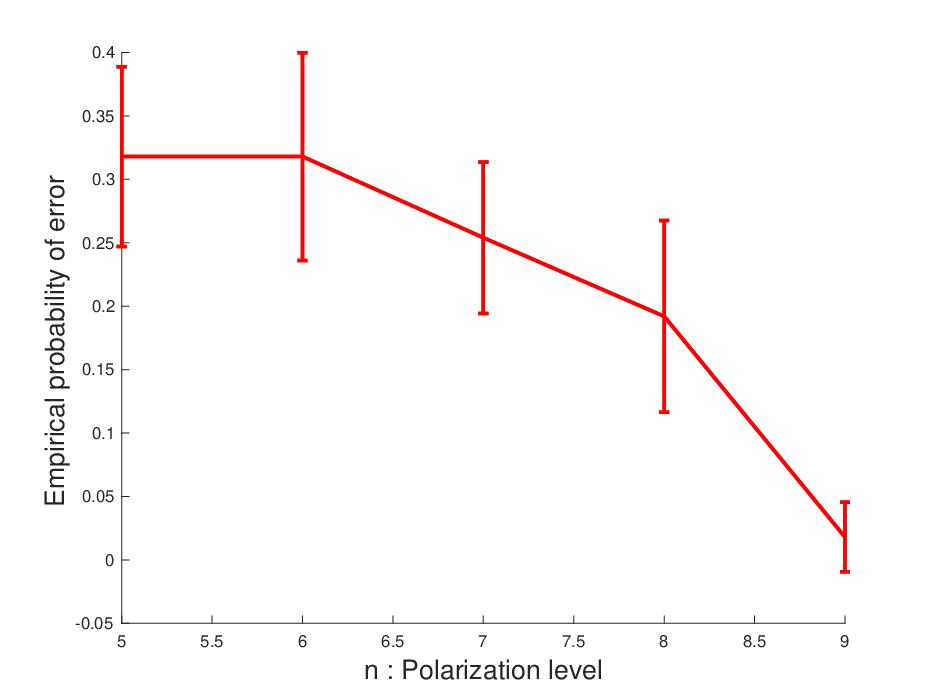
Here we provide a numerical simulations of the error probability given a deadline for the computation. We assume that the runtime distributions are i.i.d. Uniform and the rate is , implying that . We set the deadline as where , perform 10 independent trials and calculate the empirical probability of decoding error. Figure I shows that the empirical error probability as a function of the polarization level , where the corresponding number of workers is . The error bars represent one standard deviation. It can be observed that the error probability decreases to zero sharply as predicted by Theorem 4.
VII-D Experiments on Amazon Web Services (AWS)
Here we illustrate an application of computational polarization to computation times obtained from AWS Lambda serverless computing platform. Serverless computing is an emerging architectural paradigm that presents a compelling option for dynamic data intensive problems. Serverless computing relies on stateless functions that are automatically scheduled by the cloud infrastructure. Thus, they obviate the need for the provider to explicitly configure, deploy, and manage long-term compute units. We consider a distributed matrix multiplication task with random data matrices, where we employ worker nodes with rate set to . In Figure 23, we plot the runtime distribution of uncoded computation, computational polarization and MDS coded computation. It can be observed that the overall runtime of the proposed scheme is very close to MDS coded computing. However, the decoding process is significantly faster, especially when the number of worker nodes is very large.

(a) Uncoded

(b) Computational Polarization

(c) MDS coded
VIII Conclusion
We presented a resilient computing framework that extends the channel polarization phenomenon in an algorithmic sense and leverages a similar recursive construction. The proposed method creates virtual workers with a wide spectrum of runtimes by applying a split operation in a similar spirit to Polar Codes. Unlike polar codes, the polarization takes place over real valued random variables, and do not converge to discrete extremes. Instead, we have shown that the runtime distributions of the workers form a Banach space valued martingale and converge to Dirac delta measure. In this sense, the convergence is towards the extreme points of the total variation ball over the space of Radon measures. Moreover, we have shown an application of Fano’s inequality to lower bound the probability of successful recovery of the overall computation. We showed that the proposed computational polarization scheme achieves information theoretically optimal overall runtime. The major advantage of the computational polarization is the negligible decoding complexity, which only involves addition and subtraction operations over the reals. This is in contrast to other coding schemes such as MDS codes. We leave extending the proposed method to computing nonlinear functions as an important future work, where the developed convergence theory can be used. Notable examples of distributed nonlinear computations that can benefit from Computational Polarization include solving linear systems and convex optimization problems [21, 22, 23], and training neural networks [24]. Another interesting research direction is investigating applications of the Banach space martingales in traditional Polar Codes and improving the existing convergence analysis.
IX Proofs
Proof of Lemma 1.
We now verify the adjoint property. Suppose that and are two probability densities and consider the space inner-product
Finally, noting that the preceding expression equals
we prove that is the adjoint of the operator . ∎
Proof of Theorem 6.
Using the definition (36), we expand as follows
Integrating both sides, we obtain
Noting the relation
which follows from the functional update in (36), and , we express the preceding equality as
| (45) |
Let us define the deterministic sequence as
where the second equality follows from Fubini’s theorem, noting that and the integrand is absolutely integrable, i.e.,
We may express by another application of Fubini’s theorem as
which follows from the absolute integrability, i.e.,
by our assumption.
Using the definition of , combining the expression for above with the relation (45), we obtain
| (46) |
Next, we consider the convergence of the sequence . Note that
since in (46). Furthermore the sequence is bounded since we have
The first inequality follows from for all . Moreover, since the functional process (36) is a martingale, it holds that
which shows that , where . Noting that is bounded and monotone, we apply monotone convergence theorem, which shows that the sequence has a finite limit. Therefore we have
Combining the preceding result with (46), we obtain
This proves the first claimed result Consequently, an application of Markov’s inequality yields that
for any fixed scalar . Applying the previous result on the right-hand-side we obtain
which completes the proof of the theorem. We further note that
by Jensen’s inequality, and the preceding probabilistic bounds also apply to . ∎
Proof of Theorem 8.
We consider with the representation and expand as follows
It follows that for all and since we have
| (47) |
Furthermore, note that , hence for every fixed value of , is bounded and monotone. Consequently, by monotone convergence theorem, and the limit exists. This was noted by [16], where a simple proof of polarization using the monotone convergence theorem was presented. We then introduce the following function as in [16]
Note that for all and . Using the above definition, we obtain the following lower bound
Now we plugin the above lower bound in the earlier expression for and obtain
Taking supremum over both sides in the above expression, we get
| (48) |
On the other hand, Theorem 7 shows that, for a fixed value of , converges to a limiting random variable almost surely, which satisfies with probability one. Therefore, we have
| (49) |
where the last equality follows from the martingale property of the process .
Now let us fix , and note that the sequence of functions satisfies
Consequently, Dini’s theorem (see e.g. [25]) can be applied to obtain that
where we have applied triangle inequality in the second line. Combining the above result with the bound in (48), we conclude that
which completes the proof. ∎
Proof of Theorem 9.
We define the following difference function as
Using the functional update equation (41), we first establish that the difference function satisfies
where we have used the inequalities and . Plugging in the form of the functional update in (41) shows that the difference function further satisfies the following relation
Next we consider the random variable , which satisfies
Calculating the expected value of we obtain
Recursively applying the above inequality we obtain
More generally, for any satisfying , we have
Recursively applying the final inequality above, we obtain
Now we apply Markov’s inequality to the random variable and obtain the inequality
Using the earlier expression for the expectation on the right-hand-side, we obtain
Setting , we obtain the bound
This completes the proof. The above bound is effective as , when and . ∎
Proof of Theorem 10.
We begin by proving the following auxiliary lemmas to establish the claimed result.
Lemma 4.
For a fixed , the condition implies that
Proof.
Note that is a factorization of the polynomial , where and are the roots given by
The above roots are real valued and satisfy for . The condition implies that . Rearranging the preceding condition implies that The condition implies that ∎
Lemma 5.
For every fixed , and any it holds that
| (50) |
Lemma 6.
Suppose that , then we have
Lemma 7.
Suppose that , then we have

Suppose that we have for some . In particular, Lemma 5 guarantees the existence of an such that this assumption holds with high probability. Further suppose that there exists such that for all the preceding inequality holds. More precisely, consider that the condition
| (51) |
holds.
Now we consider any . We can apply Lemma 4 to deduce that . Observe that the function obeys
and can be made arbitrarily small as as shown in Figure 24 . Let us set sufficiently small to satisfy
Note that Lemma 4 implies
Now, we consider the following two cases separately:
Combining the above two cases, we obtain the bound
Now we apply the preceding inequality recursively from to where to obtain
| (52) |
Now we focus on the exponent term in the above inequality. Taking logarithms, we get
Noting that are i.i.d. Bernoulli variables satisfying
| (53) |
We now invoke Chernoff’s bound (see, e.g., [26, p. 531]) and obtain
| (54) |
where we have used the fact that , and introduced the binary entropy function . Using the probability inequality in (54), we deduce that
with probability at least . Combining the above probabilistic bound with the earlier expression in (52) we obtain that
| (55) |
holds with the same probability. Now we verify our initial assumption in (51) that simultaneously for all using Lemma 5. Let us pick , which verifies that . By Lemma 5, the event happens with probability for a fixed value of . Applying union bound over , we obtain that the aforementioned condition (51) holds with probability at least
Now we recall the following choices
| (56) | ||||
| (57) |
The above conditions can be satisfied by letting
Then we turn to the inequality in (55), note that by our assumption in (51) and obtain
| (58) |
using (55), with the stated probability. Then note that whenever the parameter satisfies
Finally combining the earlier pieces we obtain that
| (59) |
Now let us pick . Now we set and obtain
| (60) |
where we have used the fact that By picking , we can satisfy under the conditions (56), which is required to to apply Lemma 4. We then conclude that for , the probabilistic bound in (60) is valid.
Finally, conditioned on the event under which (60) holds, we can bound as follows
where the inequality in the third line follows since the inequalities and simultaneously hold, and consequently we have the upper-bound
completing the proof of the theorem. ∎
Proof of Theorem 4.
We start with the Laplace transform rule. Let us denote the number of indices that satisfy for some by
Consequently, taking limits we obtain
| (61) |
where we have set .
We apply the log-sum-exp upper bound on the expected computational run-time as follows
where we have applied Jensen’s inequality in the last inequality.
Next, we combine the bound (61) with the preceding log-sum-exp upper bound on the expected computational run-time in the limit where . We obtain
Setting in the final inequality, we obtain
We next consider the quantile selection rule. Let us denote the number of indices that satisfy for some by .
First we obtain the asymptotic ratio
where we substituted .
Now, we note that
Next we apply Theorem 10, and obtain that
where is a constant independent of to complete the proof. ∎
Proof of Theorem 3.
Consider a uniformly generated source random variable , and let be the corresponding binary expansion. We let be equal to . Consider the matrix vector product function . We note that the choice of the vector is arbitrary and other choices are equally applicable. Clearly, is sufficient to exactly reconstruct the source . Suppose that is the encoded data for any coded computation scheme, where the rate is and the computational tasks are distributed to independent and identical worker nodes. At any fixed time instant , let denote the output of the workers, and define , e.g., an erasure event whenever the -th worker is not finished the task. Then we observe that
Therefore, the mutual information between the source and available information at time obeys
where the right-hand-side is the Shannon capacity of a memoryless binary erasure channel with erasure probability (see, e.g., [27]). Since the worker nodes are i.i.d., we immediately have
Furthermore, since is a function of , we have
Let be any estimate of based on . Next, we apply Fano’s inequality to obtain
where we have used the preceding bound on in the final inequality. Observe that whenever decoding succeeds at time and hence there exists an estimator based on such that . Therefore we have
Plugging in we obtain
∎
Proof of Lemma 2.
Taking time derivatives on both sides we obtain the probability density martingale
| (62) |
In terms of the probability density , the above update equation reduces to
Next, we plug-in the relation
which follows from , and enables us to further simply the probability density process as
| (63) |
and reach the claimed identity. ∎
Proof of Theorem 5.
As stated, we assume that the random variables and admit a continuous density. Let and be real numbers satisfying . Consider the joint cumulative density function and note that
for . Consequently, we can obtain the joint probability density of and by differentiating the above joint cumulative probability.
which holds for . Conversely, for we have . Therefore, in the case of a maximum of two independent variables, a joint distribution is transformed to the product distribution of its marginal , which is given by times the indicator function . The indicator enforces the constraint that the minimum is upper-bounded by the maximum.
We can simplify the above notation as follows. Where we defined the marginalization operator
Here the superscript indicates that we are integrating over the first variable . Similarly, define
then the update can be written equivalently as
∎
Appendix A
In this section, we restate classical convergence results for scalar martingales. We refer the reader to [28] for a detailed exposition.
Let be a probability space. We will denote by an increasing sequence of of sub--fields of . A sequence of random variables is called adapted if for all , the random variable is -measurable.
An adapted sequence of integrable real valued random variables is called an integrable submartingale if the almost sure inequality
holds for all . Such a sequence of random variables is called an integrable martingale if the preceding inequality holds with equality. A collection of random variables is called uniformly integrable if
In this case As a simple corollary, if there exists such that for all , then the collection is uniformly integrable. Moreover, if is bounded for some for all , then the collection is uniformly integrable. A martingale is called a uniformly integrable martingale if the collection of random variables is uniformly integrable.
Theorem 11.
(Almost sure convergence of scalar martingales [28]) Every integrable submartingale satisfying the condition converges almost surely to a limit which is an integrable random variable. In the case of an integrable martingale, this condition is given by .
Theorem 12.
( convergence of scalar martingales) Every martingale satisfying for some , converges almost surely to a limit , and also in , i.e., . If is a uniformly integrable martingale, then the convergence is in , i.e., and .
Appendix B
In this section, we present some auxiliary technical results regarding the convergence of Banach space valued martingales. The following result is an extension of Doob’s martingale convergence theorem to Banach space valued martingales.
Theorem 13 (Proposition V-2-8, page 107 [28]).
Let be a separable Banach space which is the dual of a separable Banach space . Then, every integrable martingale with values in which satisfies
known as Doob’s condition converges almost surely to an integrable random variable with values in .
In particular, every separable reflexive Banach space and every separable Hilbert space satisfies the requirements of the theorem. As an example spaces are reflexive provided that . However, and spaces are not reflexive.
Acknowledgment
This work was partially supported by the National Science Foundation under grants IIS-1838179, ECCS-2037304, DMS-2134248, the Army Research Office and Adobe Research. We would like to thank Erdal Arikan, Burak Bartan and Orhan Arikan for insightful discussions and their valuable feedback on this work. We are grateful to Burak Bartan for his assistance in numerical simulations and Neophytos Charalambides for proofreading the manuscript. We also thank anonymous reviewers for their constructive comments.
References
- [1] M. Zaharia, M. Chowdhury, M. J. Franklin, S. Shenker, and I. Stoica, “Spark: Cluster computing with working sets.,” HotCloud, vol. 10, no. 10-10, p. 95, 2010.
- [2] J. Dean and S. Ghemawat, “Mapreduce: simplified data processing on large clusters,” Communications of the ACM, vol. 51, no. 1, pp. 107–113, 2008.
- [3] K. Lee, M. Lam, R. Pedarsani, D. Papailiopoulos, and K. Ramchandran, “Speeding up distributed machine learning using codes,” IEEE Transactions on Information Theory, vol. 64, no. 3, pp. 1514–1529, 2017.
- [4] S. Li, M. A. Maddah-Ali, Q. Yu, and A. S. Avestimehr, “A fundamental tradeoff between computation and communication in distributed computing,” IEEE Transactions on Information Theory, vol. 64, no. 1, pp. 109–128, 2017.
- [5] R. Tandon, Q. Lei, A. G. Dimakis, and N. Karampatziakis, “Gradient coding,” arXiv preprint arXiv:1612.03301, 2016.
- [6] S. Li, S. Avestimehr, et al., “Coded computing,” Foundations and Trends® in Communications and Information Theory, vol. 17, no. 1, pp. 1–148, 2020.
- [7] Q. Yu, M. Maddah-Ali, and S. Avestimehr, “Polynomial codes: an optimal design for high-dimensional coded matrix multiplication,” in Advances in Neural Information Processing Systems, pp. 4403–4413, 2017.
- [8] E. Arikan, “Channel polarization: A method for constructing capacity-achieving codes for symmetric binary-input memoryless channels,” IEEE Transactions on Information Theory, vol. 55, no. 7, pp. 3051–3073, 2009.
- [9] B. Bartan and M. Pilanci, “Straggler resilient serverless computing based on polar codes,” in 2019 57th Annual Allerton Conference on Communication, Control, and Computing (Allerton), pp. 276–283, IEEE, 2019.
- [10] F. J. MacWilliams and N. J. A. Sloane, The theory of error correcting codes, vol. 16. Elsevier, 1977.
- [11] J. Hadar and W. R. Russell, “Rules for ordering uncertain prospects,” The American economic review, vol. 59, no. 1, pp. 25–34, 1969.
- [12] V. S. Bawa, “Optimal rules for ordering uncertain prospects,” Journal of Financial Economics, vol. 2, no. 1, pp. 95–121, 1975.
- [13] J. E. Gentle, Computational statistics, vol. 308. Springer, 2009.
- [14] G. B. Folland, Real analysis: modern techniques and their applications, vol. 40. John Wiley & Sons, 1999.
- [15] A. W. van der Vaart, Asymptotic statistics. Cambridge, UK: Cambridge University Press, 1998.
- [16] M. Alsan and E. Telatar, “A simple proof of polarization and polarization for non-stationary memoryless channels,” IEEE Transactions on Information Theory, vol. 62, no. 9, pp. 4873–4878, 2016.
- [17] E. Arikan and E. Telatar, “On the rate of channel polarization,” in 2009 IEEE International Symposium on Information Theory, pp. 1493–1495, IEEE, 2009.
- [18] S. H. Hassani, K. Alishahi, and R. L. Urbanke, “Finite-length scaling for polar codes,” IEEE Transactions on Information Theory, vol. 60, no. 10, pp. 5875–5898, 2014.
- [19] A. Mallick, M. Chaudhari, U. Sheth, G. Palanikumar, and G. Joshi, “Rateless codes for near-perfect load balancing in distributed matrix-vector multiplication,” Proceedings of the ACM on Measurement and Analysis of Computing Systems, vol. 3, no. 3, pp. 1–40, 2019.
- [20] A. Soro and J. Lacan, “Fnt-based reed-solomon erasure codes,” in 2010 7th IEEE Consumer Communications and Networking Conference, pp. 1–5, IEEE, 2010.
- [21] M. Pilanci and M. J. Wainwright, “Randomized sketches of convex programs with sharp guarantees,” IEEE Trans. Info. Theory, vol. 9, pp. 5096–5115, September 2015.
- [22] M. Pilanci and M. J. Wainwright, “Newton sketch: A near linear-time optimization algorithm with linear-quadratic convergence,” SIAM Journal on Optimization, vol. 27, no. 1, pp. 205–245, 2017.
- [23] J. Lacotte and M. Pilanci, “Effective dimension adaptive sketching methods for faster regularized least-squares optimization,” arXiv preprint arXiv:2006.05874, 2020.
- [24] M. Pilanci and T. Ergen, “Neural networks are convex regularizers: Exact polynomial-time convex optimization formulations for two-layer networks,” in International Conference on Machine Learning, pp. 7695–7705, PMLR, 2020.
- [25] W. Rudin, Principles of Mathematical Analysis. New York: McGraw-Hill, 1964.
- [26] R. G. Gallager, Information Theory and Reliable Communication. New York, NY: John Wiley & Sons, 1968.
- [27] T. M. Cover, Elements of information theory. John Wiley & Sons, 1999.
- [28] J. Neveu, Discrete-parameter martingales, vol. 10. North-Holland Amsterdam, 1975.