跳到论文正文
W Papers独立论文阅读器 arXiv:2109.03847 论文正文 计算阅读时间 · 0%
引用这篇论文根据当前论文元数据生成,正式投稿前建议核对。


License: arXiv.org perpetual non-exclusive license
arXiv:2109.03847v2 [quant-ph] 21 Jul 2022

Quantum and classical dynamical semigroups of superchannels and semicausal channelsPreprint: AIP/123-QED

Markus Hasenöhrl Email: m.hasenoehrl@tum.de Affiliation:  Department of Mathematics, Technical University of Munich, Garching, Germany
Munich Center for Quantum Science and Technology (MCQST), Munich, Germany
   Matthias C. Caro Email: caro@ma.tum.de Affiliation:  Department of Mathematics, Technical University of Munich, Garching, Germany
Munich Center for Quantum Science and Technology (MCQST), Munich, Germany
August 11, 2026
Abstract

Quantum devices are subject to natural decay. We propose to study these decay processes as the Markovian evolution of quantum channels, which leads us to dynamical semigroups of superchannels. A superchannel is a linear map that maps quantum channels to quantum channels, while satisfying suitable consistency relations. If the input and output quantum channels act on the same space, then we can consider dynamical semigroups of superchannels. No useful constructive characterization of the generators of such semigroups is known. We characterize these generators in two ways: First, we give an efficiently checkable criterion for whether a given map generates a dynamical semigroup of superchannels. Second, we identify a normal form for the generators of semigroups of quantum superchannels, analogous to the GKLS form in the case of quantum channels. To derive the normal form, we exploit the relation between superchannels and semicausal completely positive maps, reducing the problem to finding a normal form for the generators of semigroups of semicausal completely positive maps. We derive a normal for these generators using a novel technique, which applies also to infinite-dimensional systems. Our work paves the way to a thorough investigation of semigroups of superchannels: Numerical studies become feasible because admissible generators can now be explicitly generated and checked. And analytic properties of the corresponding evolution equations are now accessible via our normal form.

I Introduction and Motivation

Anybody who has ever owned an electronic device knows: These devices have a finite lifespan after which they stop working properly. At least from a consumer perspective, a long lifespan is a desirable property for such devices. Thus, it is important for an engineer to know which kind of decay processes can affect a device, in order to suppress them by an appropriate design. Certainly, these considerations will also become important for the design of quantum devices. We therefore propose to study systematically the decay processes that quantum devices can be subject to.

In this work, we take a first step in this direction by deriving the general form of linear time-homogeneous master equations that govern how quantum channels behave when inserted into a circuit board at different points in time. This leads to the study of dynamical semigroups of superchannels. Here, superchannels are linear transformations between quantum channels Chiribella et al. 2008a.

Refer to caption
Figure 1: Estimating the transmissivity of a material under the influence of an influx of particles into the regions between the components.

Let us consider a concrete example, see Fig. 1. Suppose we are trying to estimate the optical transmissivity of some material (MM), which we assume to depend on the polarization of the incident light. A simple approach is to send photons from a light source (SS) through the material and to count how many photons arrive a the detector (DD). We model the material by a quantum channel TMT_{M}, acting on the states of photons described as three-level systems, with the levels corresponding to vacuum, horizontal, and vertical polarization. In an idealized world, with a perfect vacuum in the regions between the source, the material, and the detector, we can infer the transmissivity from the measurement statistics of the state TM​(σ)T_{M}(\sigma), where σ\sigma is the state of the photon emitted from the source. However, in a more realistic scenario, even though we might have created an (almost) perfect vacuum between the devices at construction time, some particles are leaked into that region over time. Then, interactions between the photons and these particles might occur, causing absorption or a change in polarization. Hence, the situation is no longer described accurately by TMT_{M} alone, but also requires a description of the particle-filled regions.

To find such a description, we us argue that the effect of particles in some region (here, either between SS and MM; or MM and DD) can be modeled by a quantum dynamical semigroup, parametrized by the particle density δ\delta. If the particle density is reasonably low and QδQ_{\delta} is the quantum channel describing the effect of the particles on the incident light at a given δ\delta, then, as explained in Fig. 2, QδQ_{\delta} satisfies the semigroup property Qδ1+δ2=Qδ1∘Qδ2Q_{\delta_{1}+\delta_{2}}=Q_{\delta_{1}}\circ Q_{\delta_{2}}.

Refer to caption
Figure 2: If the particle density is low, then the incident photon interacts with the particles in the region sequentially and independently. The effect of a single interaction can be described by a channel Δ​Q\Delta Q. Hence, the state after the first interaction is Δ​Q​(σ)\Delta Q(\sigma), the state after the second interaction is Δ​Q​(Δ​Q​(σ))\Delta Q(\Delta Q(\sigma)), and so forth. The number of interactions is given by the product of the particle density δ\delta and the volume VV. Hence, the effect of an region with fixed volume is described by the channel Qδ=(Δ​Q)δ​VQ_{\delta}=(\Delta Q)^{\delta V}. It follows that if δ=δ1+δ2\delta=\delta_{1}+\delta_{2}, then Qδ1+δ2=(Δ​Q)δ1​V​(Δ​Q)δ2​V=Qδ1∘Qδ2Q_{\delta_{1}+\delta_{2}}=(\Delta Q)^{\delta_{1}V}(\Delta Q)^{\delta_{2}V}=Q_{\delta_{1}}\circ Q_{\delta_{2}}. The semigroup property for real δ\delta can then be obtained in the continuum limit.

Furthermore, if there are no particles then there should be no effect. Hence, Q0=idQ_{0}=\mathrm{id}. After adding continuity in the parameter δ\delta as a further natural assumption, the family {Qδ}δ≥0\{Q_{\delta}\}_{\delta\geq 0} forms a quantum dynamical semigroup. That is, we can write Qδ=eL​δQ_{\delta}=e^{L\delta}, for some generator LL in GKLS-form.

If we assume in our example that particles of type AA are leaked into the region between SS and MM at a rate γA\gamma_{A} and that particles of type BB are leaked into the region between MM and DD at a rate γB\gamma_{B}, then the overall channel describing the transformation that emitted photons undergo at time tt is given by

S^t​(TM)=eγB​LB​t∘TM∘eγA​LA​t,\displaystyle\hat{S}_{t}(T_{M})=e^{\gamma_{B}L_{B}t}\circ T_{M}\circ e^{\gamma_{A}L_{A}t},

where LAL_{A} and LBL_{B} are the generators of the dynamical semigroups describing the effect of the particles in the respective regions.

We note that at any fixed time, S^t\hat{S}_{t} interpreted as a map on quantum channels is a superchannel written in ‘circuit’-form. This means, that S^t\hat{S}_{t} describes a transformation of quantum channels implemented via pre- and post-processing. Furthermore, S^t​(TM)\hat{S}_{t}(T_{M}) can be determined by solving the time-homogenous master equation

dd​t​T​(t)=L^​(T​(t)),\displaystyle\frac{d}{dt}T(t)=\hat{L}(T(t)),

where L^​(T)=γA​LA∘T+γB​T∘LB\hat{L}(T)=\gamma_{A}L_{A}\circ T+\gamma_{B}T\circ L_{B}, with initial condition T⁡(0)=TMT(0)=T_{M}. In other words, we have

S^t=eL^​t\displaystyle\hat{S}_{t}=e^{\hat{L}t}

and thus the family {S^t}t≥0\{\hat{S}_{t}\}_{t\geq 0} forms a dynamical semigroup of superchannels.

By inductive reasoning, we thus arrive at our central physical hypothesis: Decay-processes of quantum devices with some sort of influx are well described by dynamical semigroups of superchannels. It follows that such decay-processes can be understood by characterizing dynamical semigroups of superchannels. Such a characterization is the main goal of our work.

In particular, we aim to understand dynamical semigroups of superchannels in terms of their generators. We characterize these generators fully by providing two results: First, we give an efficiently checkable criterion for whether a given map generates a dynamical semigroup of superchannels. Second, we identify a normal form for the generators of semigroups of quantum superchannels, analogous to the GKLS form in the case of quantum channels. Interestingly, we find that the most general form of dynamical semigroups of superchannels goes beyond the simple introductory example above.

We arrive at these results through a path (see Fig. 3) that also illuminates the connection to the classical case. We start by studying dynamical semigroups of classical superchannels, which (analogously to quantum superchannels being transformations between quantum channels) are transformations between stochastic matrices. We do so by establishing a one-to one correspondence between classical superchannels and certain classical semicausal channels, that is, stochastic matrices on a bipartite system (A​BAB) that do not allow for communication from BB to AA (see Definition IV.2). We can then obtain a full characterization of the generators of semigroups of classical superchannels by characterizing generators of semigroups of classical semicausal maps first and then translating the results back to the level of superchannels. The study of (dynamical semigroups of) classical superchannels and classical semicausal channels is the content of Section IV.

Refer to caption
Figure 3: Schematic of the concepts studied in this work.

Armed with the intuition obtained from the classical case, we then go on to study the quantum case. We start by characterizing the generators of semigroups of semicausal Beckman et al. 2001 completely positive maps (CP-maps) – our main technical result, and one of independent interest. This characterization can be obtained from the classical case by a ‘quantization’-procedure that allows us to see exactly which features of semigroups of semicausal CP-maps are “fully quantum.” Dynamical semigroups of semicausal CP-maps are discussed Section V.2. Finally, in Section V.3, we use the one-to one correspondence (via the quantum Choi–Jamiołkowski isomorphism) between certain semicausal CP-maps and quantum superchannels to obtain a full characterization of the generators of semigroups of quantum superchannels. While the classical section (IV) and the quantum section (V) are heuristically related, they are logically independent and can be read independently.

This work is structured as follows. In the remainder of this section, we discuss results related to ours. Section II contains an overview over our main results. In Section III, we recall relevant notions from functional analysis and quantum information, as well as some notation. The (logically) independent sections IV and V comprise the main body of our paper, containing complete statements and proofs of our results on dynamical semigroups of superchannels and semicausal channels. We study the classical case in Section IV and the quantum case in Section V. Finally, we conclude with a summary and an outlook to future research in Section VI.

I.1 Related work

The study of quantum superchannels goes back to Chiribella et al. 2008a and has since evolved to the study of higher-order quantum maps Chiribella et al. 2008b; Chiribella et al. 2009; Bisio and Perinotti 2019. A peculiar feature of higher-order quantum theory is that it allows for indefinite causal order Oreshkov et al. 2012; Chiribella et al. 2013a. However, it was recently discovered that the causal order is preserved under (certain) continuous evolutions Castro-Ruiz et al. 2018; Selby et al. 2020. It therefore seems interesting to study continuous evolutions of higher-order quantum maps systematically. Our work can be seen as an initial step into his direction.

The study of (semi-)causal and (semi-)localizable quantum channels goes back to Beckman et al. 2001. By proving the equivalence of semicausality and semilocalizability for quantum channels, Eggeling et al. 2002 resolved a conjecture raised in Beckman et al. 2001 (and attributed to DiVincenzo). Later, Piani et al. 2006 provided an alternative proof for this equivalence, and further investigated causal and local quantum operations.

II Results

We give an overview over our answers to the questions identified in the previous section. In our first result, we identify a set of constraints that a linear map satisfies if and only if it generates a semigroup of quantum superchannels.

Result 1.1 (Lemma V.17 - Informal).

Checking whether a linear map L^:ℬ⁡(ℬ⁡(ℋA),ℬ⁡(ℋB))→ℬ⁡(ℬ⁡(ℋA),ℬ⁡(ℋB))\hat{L}:\mathcal{B}(\mathcal{B}(\mathcal{H}_{A});\mathcal{B}(\mathcal{H}_{B}))\to\mathcal{B}(\mathcal{B}(\mathcal{H}_{A});\mathcal{B}(\mathcal{H}_{B})) generates a semigroup of quantum superchannels can be phrased as a semidefinite constraint satisfaction problem.

Therefore, we can efficiently check whether a given linear map is a valid generator of a semigroup of quantum superchannels. We can even solve optimization problems over such generators in terms of semidefinite programs. Thereby, this first characterization of generators of semigroups of quantum superchannels facilitates working with them computationally.

As our second result, we determine a normal form for generators of semigroups of quantum superchannels. Similar to the GKLS-form, we decompose the generator into a “dissipative part” and a “Hamiltonian part,” where the latter generates a semigroup of invertible superchannels such that the inverse is a superchannel as well.

Result 1.2 (Theorem V.18 - Informal).

A linear map L^:ℬ⁡(ℬ⁡(ℋA),ℬ⁡(ℋB))→ℬ⁡(ℬ⁡(ℋA),ℬ⁡(ℋB))\hat{L}:\mathcal{B}(\mathcal{B}(\mathcal{H}_{A});\mathcal{B}(\mathcal{H}_{B}))\to\mathcal{B}(\mathcal{B}(\mathcal{H}_{A});\mathcal{B}(\mathcal{H}_{B})) generates a semigroup of quantum superchannels if and only if it can be written as L^​(T)=D^​(T)+H^​(T)\hat{L}(T)=\hat{D}(T)+\hat{H}(T), where the “Hamiltonian part” is of the form

H^​(T)​(ρ)=−i⁡[HB,T⁡(ρ)]−i​T​([HA,ρ]),\displaystyle\hat{H}(T)(\rho)=-i[H_{B},T(\rho)]-iT([H_{A},\rho]),

with local Hamiltonians HBH_{B} and HAH_{A}, and where the “dissipative part” is of the form D^​(T)​(ρ)=trE​[D^′​(T)​(ρ)]\hat{D}(T)(\rho)=\mathrm{tr}_{E}\left[\hat{D}^{\prime}(T)(\rho)\right], where

D^′​(T)​(ρ)\displaystyle\hat{D}^{\prime}(T)(\rho) =U⁡(T⊗idE)​(A⁡(ρ⊗σ)​A†)​U†\displaystyle=U(T\otimes\mathrm{id}_{E})(A(\rho\otimes\sigma)A^{\dagger})U^{\dagger} −12​(T⊗idE)​({A†​A,ρ⊗σ})\displaystyle-\frac{1}{2}(T\otimes\mathrm{id}_{E})(\left\{A^{\dagger}A\,,\,\rho\otimes\sigma\right\}) (1a)
+B⁡(T⊗idE)​(ρ⊗σ)​B†\displaystyle+B(T\otimes\mathrm{id}_{E})(\rho\otimes\sigma)B^{\dagger} −12​{B†​B,(T⊗idE)​(ρ⊗σ)}\displaystyle-\frac{1}{2}\left\{B^{\dagger}B\,,\,(T\otimes\mathrm{id}_{E})(\rho\otimes\sigma)\right\} (1b)
+[U⁡(T⊗idE)​(A⁡(ρ⊗σ)),B†]\displaystyle+\left[U(T\otimes\mathrm{id}_{E})(A(\rho\otimes\sigma))\,,\,B^{\dagger}\right] +[B,(T⊗idE)​((ρ⊗σ)​A†)​U†],\displaystyle+\left[B\,,\,(T\otimes\mathrm{id}_{E})((\rho\otimes\sigma)A^{\dagger})U^{\dagger}\right], (1c)

with unitary UU and arbitrary AA and BB.

The “dissipative part” consists of three terms: Term (1a) itself generates a semigroup of superchannels (for B=0B=0), with the interpretation that the transformed channel (S^t​(T)\hat{S}_{t}(T)) arises due to the stochastic application of T↦trE​[U⁡(T⊗idE)​(A⁡(ρ⊗σ)​A†)​U†]T\mapsto\mathrm{tr}_{E}\left[U(T\otimes\mathrm{id}_{E})(A(\rho\otimes\sigma)A^{\dagger})U^{\dagger}\right] at different points in time (Dyson series expansion). Term (1b) itself generates a semigroup of superchannels (for A=0A=0) of the form S^t​(T)=eLB​t∘T\hat{S}_{t}(T)=e^{L_{B}t}\circ T, where LBL_{B} is a generator of a quantum dynamical semigroup (and hence in GKLS-form). Term (1c) is a “superposition” term, which is harder to interpret. It will become apparent from the path taken via the ‘quantization’ of semicausal semigroups that this term is a pure quantum feature with no classical analogue. Therefore, the presence of (1c) can be regarded as one of our main findings. It is also worth noting that the normal form in Result 1.2 is more general than the form of of the generator we found in our introductory example. Hence, nature allows for more general decay-processes than the simple ones with an independent influx of particles before and after the target object. We also complement this structural result by an algorithm that determines the operators UU, AA, BB, HAH_{A} and HBH_{B}, if the conditions in Result 1.1 are met.

The proof of these results relies on the relation (via the Choi-Jamiołkowski isomorphism) between superchannels and semicausal CP-maps. Our next findings – and from a technical standpoint our main contributions – are the corresponding results for semigroups of semicausal CP-maps.

Result 2.1 (Lemma V.5 - Informal).

Checking whether a linear map L:ℬ⁡(ℋA⊗ℋB)→ℬ⁡(ℋA⊗ℋB)L:\mathcal{B}(\mathcal{H}_{A}\otimes\mathcal{H}_{B})\to\mathcal{B}(\mathcal{H}_{A}\otimes\mathcal{H}_{B}) generates a semigroup of B↛AB\not\to A semicausal CP-maps can be phrased as a semidefinite constraint satisfaction problem for its Choi-matrix.

Based on this insight, we can efficiently check whether a given linear map is a valid generator of a semigroup of semicausal CP-maps.

Since semigroups of semicausal CP-maps are in particular semigroups of CP-maps, our normal form for generators giving rise to semigroups of semicausal CP-maps is a refining of the the GKLS-form.

Result 2.2 (Theorem V.6 - Informal).

A linear map L:ℬ⁡(ℋA⊗ℋB)→ℬ⁡(ℋA⊗ℋB)L:\mathcal{B}(\mathcal{H}_{A}\otimes\mathcal{H}_{B})\to\mathcal{B}(\mathcal{H}_{A}\otimes\mathcal{H}_{B}) generates a semigroup of B↛AB\not\to A semicausal CP-maps (in the Heisenberg picture) if and only if it can be written as L⁡(X)=Φ⁡(X)−K†​X−X​KL(X)=\Phi(X)-K^{\dagger}X-XK, where the CP part Φ\Phi is of the form

Φ⁡(X)\displaystyle\Phi(X) =V†​(X⊗𝟙E)​V, with ​V=(𝟙A⊗U)​(A⊗𝟙B)+(𝟙A⊗B),\displaystyle=V^{\dagger}\left(X\otimes\mathds{1}_{E}\right)V,\text{ with }V=(\mathds{1}_{A}\otimes U)(A\otimes\mathds{1}_{B})+(\mathds{1}_{A}\otimes B),

with a unitary U∈ℬ⁡(ℋE⊗ℋB,ℋB⊗ℋE)U\in\mathcal{B}(\mathcal{H}_{E}\otimes\mathcal{H}_{B};\mathcal{H}_{B}\otimes\mathcal{H}_{E}) and arbitrary A∈ℬ⁡(ℋA,ℋA⊗ℋE)A\in\mathcal{B}(\mathcal{H}_{A};\mathcal{H}_{A}\otimes\mathcal{H}_{E}) and B∈ℬ⁡(ℋB,ℋB⊗ℋE)B\in\mathcal{B}(\mathcal{H}_{B};\mathcal{H}_{B}\otimes\mathcal{H}_{E}), and the KK in the non-CP part is of the form

K\displaystyle K =(𝟙A⊗B†​U)​(A⊗𝟙B)+12​𝟙A⊗B†​B+KA⊗𝟙B+𝟙A⊗i​HB,\displaystyle=(\mathds{1}_{A}\otimes B^{\dagger}U)(A\otimes\mathds{1}_{B})+\frac{1}{2}\mathds{1}_{A}\otimes B^{\dagger}B+K_{A}\otimes\mathds{1}_{B}+\mathds{1}_{A}\otimes iH_{B},

with a self-adjoint HBH_{B} and an arbitrary KAK_{A}.

This characterization has both computational and analytical implications: On the one hand, it provides a recipe for describing semicausal GKLS generators in numerical implementations. On the other hand, the constructive characterization of semicausal GKLS generators makes a more detailed analysis of their (e.g., spectral) properties tractable. It is also worth noting that in Result 2.2 we can allow for (separable) infinite-dimensional spaces. In the finite-dimensional case, we also provide an algorithm to compute the operators UU, AA, BB, KAK_{A} and HBH_{B}, if the conditions of Result 2.1 are met.

Let us now turn to the corresponding results in the classical case. Here, instead of looking at (semigroups of) CP-maps and quantum channels, we look at (entry-wise) non-negative matrices and row-stochastic matrices (see Section III and Section IV for details) that we assume to act on ℝ𝕏\mathbb{R}^{\mathbb{X}}, for (finite) alphabets 𝕏∈{𝔸,𝔹,𝔼}\mathbb{X}\in\{\mathbb{A},\mathbb{B},\mathbb{E}\}.

The following result is the classical analogue of Result 2.2.

Result 3 (Corollary IV.8 - Informal).

A linear map Q:ℝ𝔸⊗ℝ𝔹→ℝ𝔸⊗ℝ𝔹Q:\mathbb{R}^{\mathbb{A}}\otimes\mathbb{R}^{\mathbb{B}}\rightarrow\mathbb{R}^{\mathbb{A}}\otimes\mathbb{R}^{\mathbb{B}} generates a semigroup of (Heisenberg) B↛AB\not\to A semicausal non-negative matrices if and only if it can be written as

Q=(A⊗𝟙B)(𝟙A⊗U)−KA⊗𝟙B+∑i=1|𝔸||ai⟩⟨ai|⊗B(i),\displaystyle Q=(A\otimes\mathds{1}_{B})(\mathds{1}_{A}\otimes U)-K_{A}\otimes\mathds{1}_{B}+\sum\limits_{i=1}^{\lvert\mathbb{A}\rvert}\lvert a_{i}\rangle\langle a_{i}\rvert\otimes B^{(i)},

with a row-stochastic matrix U∈ℬ⁡(ℝ𝔹,ℝ𝔼⊗ℝ𝔹)U\in\mathcal{B}(\mathbb{R}^{\mathbb{B}};\mathbb{R}^{\mathbb{E}}\otimes\mathbb{R}^{\mathbb{B}}), a non-negative matrix A∈ℬ⁡(ℝ𝔸⊗ℝ𝔼,ℝ𝔸)A\in\mathcal{B}(\mathbb{R}^{\mathbb{A}}\otimes\mathbb{R}^{\mathbb{E}};\mathbb{R}^{\mathbb{A}}), a diagonal matrix KAK_{A} and maps B(i)∈ℬ⁡(ℝ𝔹)B^{(i)}\in\mathcal{B}(\mathbb{R}^{\mathbb{B}}) that generate semigroups of row-stochastic matrices.

We will discuss in detail how Result 2.2 arises as the ‘quantization’ of Result 3 in the paragraph following the proof of Lemma V.5. Here, we highlight that in both the quantum and the classical case, the generators of semicausal semigroups are constructed from two basic building blocks. In the quantum case, these are a B↛AB\not\to A semicausal CP-map Φs​c\Phi_{sc}, with Φs​c​(X)=Vs​c†​(X⊗𝟙E)​Vs​c\Phi_{sc}(X)=V_{sc}^{\dagger}(X\otimes\mathds{1}_{E})V_{sc} and Vs​c=(𝟙A⊗U)​(A⊗𝟙B)V_{sc}=(\mathds{1}_{A}\otimes U)(A\otimes\mathds{1}_{B}); and a GKLS generator of the form idA⊗B^\mathrm{id}_{A}\otimes\hat{B}. And in the classical case, they are a B↛AB\not\to A semicausal non-negative map Φs​c=(𝟙A⊗U)​(A⊗𝟙B)\Phi_{sc}=(\mathds{1}_{A}\otimes U)(A\otimes\mathds{1}_{B}); and operators of the form |ai⟩⟨ai|⊗B(i)\lvert a_{i}\rangle\langle a_{i}\rvert\otimes B^{(i)}, where B(i)B^{(i)} generates a semigroup of row-stochastic maps. The difference between the quantum case and the classical case then lies in the way the general form is constructed from the building blocks. While we simply take convex combinations of the building-blocks in the classical case, we have to take superpositions of the building-blocks, by which we mean that we need to combine the corresponding Strinespring operators, in the quantum case.

As our last result, we present the normal form for generators of semigroups of classical superchannels.

Result 4.

A linear map Q^:ℬ⁡(ℝ𝔸,ℝ𝔹)→ℬ⁡(ℝ𝔸,ℝ𝔹)\hat{Q}:\mathcal{B}(\mathbb{R}^{\mathbb{A}};\mathbb{R}^{\mathbb{B}})\rightarrow\mathcal{B}(\mathbb{R}^{\mathbb{A}};\mathbb{R}^{\mathbb{B}}) generates a semigroup of classical superchannels if and only if it can be written as

Q^(M)=U(M⊗𝟙E)A−∑i=1|𝔸|⟨𝟏A​E|Aai⟩M|ai⟩⟨ai|+∑i=1|𝔸|B(i)M|ai⟩⟨ai|,\displaystyle\hat{Q}(M)=U(M\otimes\mathds{1}_{E})A-\sum_{i=1}^{\left|\mathbb{A}\right|}\langle\bm{1}_{AE}|Aa_{i}\rangle M\lvert a_{i}\rangle\langle a_{i}\rvert+\sum_{i=1}^{\left|\mathbb{A}\right|}B^{(i)}M\lvert a_{i}\rangle\langle a_{i}\rvert,

with a column-stochastic matrix U∈ℬ⁡(ℝ𝔼⊗ℝ𝔹,ℝ𝔹)U\in\mathcal{B}(\mathbb{R}^{\mathbb{E}}\otimes\mathbb{R}^{\mathbb{B}};\mathbb{R}^{\mathbb{B}}), a non-negative matrix A∈ℬ⁡(ℝ𝔸,ℝ𝔸⊗ℝ𝔼)A\in\mathcal{B}(\mathbb{R}^{\mathbb{A}};\mathbb{R}^{\mathbb{A}}\otimes\mathbb{R}^{\mathbb{E}}), a diagonal matrix KAK_{A}, and a collection of generators of semigroups of column-stochastic matrices B(i)∈ℬ⁡(ℝ𝔹)B^{(i)}\in\mathcal{B}(\mathbb{R}^{\mathbb{B}}).

As in the quantum case, we have two kinds of evolutions: a stochastic application of M↦U⁡(M⊗𝟙E)​AM\mapsto U(M\otimes\mathds{1}_{E})A at different points in time; and a conditioned post-processing evolution of the form ∑ieB(i)​tM|ai⟩⟨ai|\sum_{i}e^{B^{(i)}t}M\lvert a_{i}\rangle\langle a_{i}\rvert. Note that there are no “superposition” terms, like (1c).

III Notation and preliminaries

In this section, we review basic notions from Functional Analysis, Quantum Information Theory, and the theory of dynamical semigroups. We also fix our notation for these settings as well as for a classical counterpart of the quantum setting.

III.1 Functional analysis

Throughout the paper, ℋ\mathcal{H} (with some subscript) denotes a (in general infinite-dimensional) separable complex Hilbert space. Whenever ℋ\mathcal{H} is assumed to be finite-dimensional, we explicitly state this assumption. We denote the Banach space of bounded linear operators with domain ℋA\mathcal{H}_{A} and codomain ℋB\mathcal{H}_{B}, equipped with the operator norm, by ℬ⁡(ℋA,ℋB)\mathcal{B}(\mathcal{H}_{A};\mathcal{H}_{B}) and write ℬ⁡(ℋ)\mathcal{B}(\mathcal{H}) for ℬ⁡(ℋ,ℋ)\mathcal{B}(\mathcal{H};\mathcal{H}). For X∈ℬ⁡(ℋA,ℋB)X\in\mathcal{B}(\mathcal{H}_{A};\mathcal{H}_{B}), the adjoint X†∈ℬ⁡(ℋB,ℋA)X^{\dagger}\in\mathcal{B}(\mathcal{H}_{B};\mathcal{H}_{A}) of XX is the unique linear operator such that ⟨ψB|X​ψA⟩=⟨X†​ψB|ψA⟩\langle\psi_{B}|X\psi_{A}\rangle=\langle X^{\dagger}\psi_{B}|\psi_{A}\rangle for all |ψA⟩∈ℋA\lvert\psi_{A}\rangle\in\mathcal{H}_{A} and all |ψB⟩∈ℋB\lvert\psi_{B}\rangle\in\mathcal{H}_{B}. Here, and throughout the paper, we use the standard Dirac notation.

An operator Y∈ℬ⁡(ℋ)Y\in\mathcal{B}(\mathcal{H}) is called self-adjoint if Y†=YY^{\dagger}=Y. A self-adjoint Y∈ℬ⁡(ℋ)Y\in\mathcal{B}(\mathcal{H}) is called positive semidefinite, denoted by Y≥0Y\geq 0, if there exists an operator Z∈ℬ⁡(ℋ)Z\in\mathcal{B}(\mathcal{H}), such that Y=Z†​ZY=Z^{\dagger}Z. If YY is positive semidefinite, then there exists a unique positive semidefinite operator Y\sqrt{Y}, such that Y=Y​YY=\sqrt{Y}\sqrt{Y} (Reed and Simon 1980, p. 196). The operator Y\sqrt{Y} is called the square-root of YY. The absolute value |Y|∈ℬ⁡(ℋ)\left|Y\right|\in\mathcal{B}(\mathcal{H}) of YY is defined by |Y|=Y†​Y\left|Y\right|=\sqrt{Y^{\dagger}Y}.

We define the set of trace-class operators 𝒮1​(ℋA,ℋB)={ρ∈ℬ⁡(ℋA,ℋB)|tr⁡[|ρ|]<∞}\mathcal{S}_{1}(\mathcal{H}_{A};\mathcal{H}_{B})=\left\{\rho\in\mathcal{B}(\mathcal{H}_{A};\mathcal{H}_{B})\,\middle|\,\mathrm{tr}\left[\left|\rho\right|\right]<\infty\right\}, which becomes a Banach space when endowed with the norm ‖ρ‖1:=tr⁡[|ρ|]\left\lVert\rho\right\rVert_{1}:=\mathrm{tr}\left[\left|\rho\right|\right]. We write 𝒮1​(ℋ)\mathcal{S}_{1}(\mathcal{H}) for 𝒮1​(ℋ,ℋ)\mathcal{S}_{1}(\mathcal{H};\mathcal{H}). The set 𝒮1​(ℋA,ℋB)\mathcal{S}_{1}(\mathcal{H}_{A};\mathcal{H}_{B}) satisfies the two-sided ∗-ideal property: If ρ∈𝒮1​(ℋA,ℋB)\rho\in\mathcal{S}_{1}(\mathcal{H}_{A};\mathcal{H}_{B}) and Y∈ℬ⁡(ℋA,ℋB)Y\in\mathcal{B}(\mathcal{H}_{A};\mathcal{H}_{B}), then ρ†∈𝒮1​(ℋB,ℋA)\rho^{\dagger}\in\mathcal{S}_{1}(\mathcal{H}_{B};\mathcal{H}_{A}), ρ†​Y∈𝒮1​(ℋA)\rho^{\dagger}Y\in\mathcal{S}_{1}(\mathcal{H}_{A}) and Y​ρ†∈𝒮1​(ℋB)Y\rho^{\dagger}\in\mathcal{S}_{1}(\mathcal{H}_{B}).

Besides the norm topology, we will use the strong operator topology and the ultraweak topology. The strong operator topology is the smallest topology on ℬ⁡(ℋA,ℋB)\mathcal{B}(\mathcal{H}_{A};\mathcal{H}_{B}) such that for all |ψA⟩∈ℋA\lvert\psi_{A}\rangle\in\mathcal{H}_{A} the map ℬ(ℋA;ℋB)∋Y↦Y|ψA⟩∈ℋB\mathcal{B}(\mathcal{H}_{A};\mathcal{H}_{B})\ni Y\mapsto Y\lvert\psi_{A}\rangle\in\mathcal{H}_{B} is continuous, where ℋB\mathcal{H}_{B} is equipped with the norm topology. The ultraweak topology on ℬ⁡(ℋA,ℋB)\mathcal{B}(\mathcal{H}_{A};\mathcal{H}_{B}) is the smallest topology such that the map ℬ⁡(ℋA,ℋB)∋Y↦tr⁡[ρ†​Y]∈ℂ\mathcal{B}(\mathcal{H}_{A};\mathcal{H}_{B})\ni Y\mapsto\mathrm{tr}\left[\rho^{\dagger}Y\right]\in\mathbb{C} is continuous for all ρ∈𝒮1​(ℋA,ℋB)\rho\in\mathcal{S}_{1}(\mathcal{H}_{A};\mathcal{H}_{B}). Since ℋA\mathcal{H}_{A} and ℋB\mathcal{H}_{B} are separable, so is 𝒮1​(ℋB,ℋA)\mathcal{S}_{1}(\mathcal{H}_{B};\mathcal{H}_{A}). Hence, the sequential Banach Alaoglu theorem implies that every bounded sequence in ℬ⁡(ℋA,ℋB)\mathcal{B}(\mathcal{H}_{A};\mathcal{H}_{B}) has an ultraweakly convergent subsequence. Here, we view ℬ⁡(ℋA,ℋB)\mathcal{B}(\mathcal{H}_{A};\mathcal{H}_{B}) as the continuous dual of 𝒮1​(ℋB,ℋA)\mathcal{S}_{1}(\mathcal{H}_{B};\mathcal{H}_{A}). The aforementioned results can be found in many books, e.g, (Reed and Simon 1980, ch. VI.6), however, usually only for the case ℋA=ℋB\mathcal{H}_{A}=\mathcal{H}_{B}. The general results stated above can be obtained from this case by considering ℬ⁡(ℋA,ℋB)\mathcal{B}(\mathcal{H}_{A};\mathcal{H}_{B}) and 𝒮1​(ℋA,ℋB)\mathcal{S}_{1}(\mathcal{H}_{A};\mathcal{H}_{B}) as subspaces of ℬ⁡(ℋA⊕ℋB)\mathcal{B}(\mathcal{H}_{A}\oplus\mathcal{H}_{B}) and 𝒮1​(ℋA⊕ℋB)\mathcal{S}_{1}(\mathcal{H}_{A}\oplus\mathcal{H}_{B}), respectively.

An operator V∈ℬ⁡(ℋA,ℋB)V\in\mathcal{B}(\mathcal{H}_{A};\mathcal{H}_{B}) is called an isometry if ‖V|ψA⟩‖=‖|ψA⟩‖\left\lVert V\lvert\psi_{A}\rangle\right\rVert=\left\lVert\lvert\psi_{A}\rangle\right\rVert for all |ψA⟩∈ℋA\lvert\psi_{A}\rangle\in\mathcal{H}_{A}. The (possibly empty) set of unitaries, the surjective isometries, is denoted by 𝒰⁡(ℋA,ℋB)\mathcal{U}(\mathcal{H}_{A};\mathcal{H}_{B}) and we write 𝒰⁡(ℋ)\mathcal{U}(\mathcal{H}) for 𝒰⁡(ℋ,ℋ)\mathcal{U}(\mathcal{H};\mathcal{H}). As a special notation, if ℋA′\mathcal{H}_{A}^{\prime} and ℋB′\mathcal{H}_{B}^{\prime} are closed linear subspaces of ℋA\mathcal{H}_{A} and ℋB\mathcal{H}_{B}, with (canonical) isometric embeddings 𝟙A′→A∈ℬ⁡(ℋA′,ℋA)\mathds{1}_{A^{\prime}\rightarrow A}\in\mathcal{B}(\mathcal{H}_{A}^{\prime};\mathcal{H}_{A}) and 𝟙B′→B∈ℬ⁡(ℋB′,ℋB)\mathds{1}_{B^{\prime}\rightarrow B}\in\mathcal{B}(\mathcal{H}_{B}^{\prime};\mathcal{H}_{B}), respectively, then we will write 𝒰P​(ℋA′,ℋB′)={𝟙B′→B​U​𝟙A′→A†∈ℬ⁡(ℋA,ℋB)|U∈𝒰⁡(ℋA′,ℋB′)}\mathcal{U}_{P}(\mathcal{H}_{A}^{\prime};\mathcal{H}_{B}^{\prime})=\{\mathds{1}_{B^{\prime}\rightarrow B}U\mathds{1}_{A^{\prime}\rightarrow A}^{\dagger}\in\mathcal{B}(\mathcal{H}_{A};\mathcal{H}_{B})\,|\,U\in\mathcal{U}(\mathcal{H}_{A}^{\prime};\mathcal{H}_{B}^{\prime})\} and, 𝒰P​(ℋ)\mathcal{U}_{P}(\mathcal{H}) for 𝒰P​(ℋ,ℋ)\mathcal{U}_{P}(\mathcal{H};\mathcal{H}). I.e., this is the set of partial isometries.

III.2 Flip operator, partial trace, complete positivity, and duality

The flip operator 𝔽A;B∈ℬ⁡(ℋA⊗ℋB,ℋB⊗ℋA)\mathbb{F}_{A;B}\in\mathcal{B}(\mathcal{H}_{A}\otimes\mathcal{H}_{B};\mathcal{H}_{B}\otimes\mathcal{H}_{A}) is the unique operator satisfying 𝔽A;B(|ψA⟩⊗|ψB⟩)=|ψB⟩⊗|ψA⟩\mathbb{F}_{A;B}(\lvert\psi_{A}\rangle\otimes\lvert\psi_{B}\rangle)=\lvert\psi_{B}\rangle\otimes\lvert\psi_{A}\rangle, for all |ψA⟩∈ℋ𝒜\lvert\psi_{A}\rangle\in\mathcal{H_{A}} and all |ψB⟩∈ℋB\lvert\psi_{B}\rangle\in\mathcal{H}_{B}.

The partial trace w.r.t. the space ℋA\mathcal{H}_{A} is the unique linear map trA:𝒮1​(ℋA⊗ℋB,ℋA⊗ℋC)→𝒮1​(ℋB,ℋC)\mathrm{tr}_{A}:\mathcal{S}_{1}(\mathcal{H}_{A}\otimes\mathcal{H}_{B};\mathcal{H}_{A}\otimes\mathcal{H}_{C})\rightarrow\mathcal{S}_{1}(\mathcal{H}_{B};\mathcal{H}_{C}) that satisfies tr⁡[X​trA​[ρ]]=tr⁡[(𝟙A⊗X)​ρ]\mathrm{tr}\left[X\mathrm{tr}_{A}\left[\rho\right]\right]=\mathrm{tr}\left[(\mathds{1}_{A}\otimes X)\rho\right], for all ρ∈𝒮1​(ℋA⊗ℋB)\rho\in\mathcal{S}_{1}(\mathcal{H}_{A}\otimes\mathcal{H}_{B}) and all X∈ℬ⁡(ℋC,ℋB)X\in\mathcal{B}(\mathcal{H}_{C};\mathcal{H}_{B}). If the spaces involved have subscripts, the partial trace will always be denoted with the corresponding subscript. The partial trace with respect to ρ∈𝒮1​(ℋA)\rho\in\mathcal{S}_{1}(\mathcal{H}_{A}) is the unique linear map trρ:ℬ⁡(ℋA⊗ℋB,ℋA⊗ℋC)→ℬ⁡(ℋB,ℋC)\mathrm{tr}_{\rho}:\mathcal{B}(\mathcal{H}_{A}\otimes\mathcal{H}_{B};\mathcal{H}_{A}\otimes\mathcal{H}_{C})\rightarrow\mathcal{B}(\mathcal{H}_{B};\mathcal{H}_{C}) that satisfies tr⁡[σ​trρ​[X]]=tr⁡[(ρ⊗σ)​X]\mathrm{tr}\left[\sigma\mathrm{tr}_{\rho}\left[X\right]\right]=\mathrm{tr}\left[(\rho\otimes\sigma)X\right], for all σ∈𝒮1​(ℋC,ℋB)\sigma\in\mathcal{S}_{1}(\mathcal{H}_{C};\mathcal{H}_{B}) and all X∈ℬ⁡(ℋA⊗ℋB,ℋA⊗ℋC)X\in\mathcal{B}(\mathcal{H}_{A}\otimes\mathcal{H}_{B};\mathcal{H}_{A}\otimes\mathcal{H}_{C}). Proofs of existence and uniqueness can be found in (Attal 2021a, Thm. 2.28 and Thm. 2.30), where we used again the observation that the results above follow from the usual ones for ℋB=ℋC\mathcal{H}_{B}=\mathcal{H}_{C}, by looking at operators on ℋA⊗(ℋB⊕ℋC)\mathcal{H}_{A}\otimes(\mathcal{H}_{B}\oplus\mathcal{H}_{C}).

Let T∈ℬ⁡(ℬ⁡(ℋB),ℬ⁡(ℋA))T\in\mathcal{B}(\mathcal{B}(\mathcal{H}_{B});\mathcal{B}(\mathcal{H}_{A})). The map TT is called positive if T⁡(XB)T(X_{B}) is positive semidefinite, whenever XB∈ℬ⁡(ℋB)X_{B}\in\mathcal{B}(\mathcal{H}_{B}) is positive semidefinite. For n∈ℕ0n\in\mathbb{N}_{0}, the map Tn:ℬ⁡(ℂn⊗ℋB)→ℬ⁡(ℂn⊗ℋA)T_{n}:\mathcal{B}(\mathbb{C}^{n}\otimes\mathcal{H}_{B})\rightarrow\mathcal{B}(\mathbb{C}^{n}\otimes\mathcal{H}_{A}) is uniquely defined by the requirement that Tn​(Xn⊗XB)=Xn⊗T⁡(XB)T_{n}(X_{n}\otimes X_{B})=X_{n}\otimes T(X_{B}) for all Xn∈ℬ⁡(ℂn)X_{n}\in\mathcal{B}(\mathbb{C}^{n}) and all XB∈ℬ⁡(ℋB)X_{B}\in\mathcal{B}(\mathcal{H}_{B}). The map TT is completely positive (CP) if the map TnT_{n} is positive for all n∈ℕ0n\in\mathbb{N}_{0}. A CP-map TT is called normal if TT is continuous when ℬ⁡(ℋA)\mathcal{B}(\mathcal{H}_{A}) and ℬ⁡(ℋB)\mathcal{B}(\mathcal{H}_{B}) are both equipped with the ultraweak topology. We denote the set of normal CP-maps by CPσ​(ℋB,ℋA)\mathrm{CP}_{\sigma}(\mathcal{H}_{B};\mathcal{H}_{A}) and write CPσ​(ℋ)\mathrm{CP}_{\sigma}(\mathcal{H}) for CPσ​(ℋ,ℋ)\mathrm{CP}_{\sigma}(\mathcal{H};\mathcal{H}). By the Stinespring dilation theorem (in its form for normal CP-maps), TT is a normal CP-map if and only if there exists a (separable) Hilbert space ℋE\mathcal{H}_{E} and an operator V∈ℬ⁡(ℋA,ℋB⊗ℋE)V\in\mathcal{B}(\mathcal{H}_{A};\mathcal{H}_{B}\otimes\mathcal{H}_{E}) such that for all XB∈ℬ⁡(ℋB)X_{B}\in\mathcal{B}(\mathcal{H}_{B}) we have T⁡(XB)=V†​(XB⊗𝟙E)​VT(X_{B})=V^{\dagger}(X_{B}\otimes\mathds{1}_{E})V. Furthermore, the Stinespring dilation can be chosen to be minimal, that is, the pair (V,ℋE)(V,\mathcal{H}_{E}) can be chosen such that span{(XB⊗𝟙E)V|ψA⟩|XB∈ℬ(ℋB),|ψA⟩∈ℋA}\mathrm{span}\{(X_{B}\otimes\mathds{1}_{E})V\lvert\psi_{A}\rangle\,|\,X_{B}\in\mathcal{B}(\mathcal{H}_{B}),\lvert\psi_{A}\rangle\in\mathcal{H}_{A}\} is norm-dense in ℋB⊗ℋE\mathcal{H}_{B}\otimes\mathcal{H}_{E}. Furthermore, if (V′,ℋE′)(V^{\prime},\mathcal{H}_{E}^{\prime}) is another Stinespring dilation, then there exists an isometry U∈ℬ⁡(ℋE,ℋE′)U\in\mathcal{B}(\mathcal{H}_{E};\mathcal{H}_{E}^{\prime}), such that V′=(𝟙B⊗U)​VV^{\prime}=(\mathds{1}_{B}\otimes U)V. Another equivalent characterization is the so-called Kraus form: TT is a normal CP-map if and only if there exists a countable set of operators {Li}i⊂ℬ⁡(ℋA,ℋB)\{L_{i}\}_{i}\subset\mathcal{B}(\mathcal{H}_{A};\mathcal{H}_{B}), the Kraus operators, such that for all XB∈ℬ⁡(ℋB)X_{B}\in\mathcal{B}(\mathcal{H}_{B}), we have T⁡(XB)=∑iLi†​XB​LiT(X_{B})=\sum_{i}L_{i}^{\dagger}X_{B}L_{i}, where the series converges in the strong operator topology. One can obtain Kraus operators from a Stinespring dilation (V,ℋE)(V,\mathcal{H}_{E}) by choosing an orthonormal basis {|ei⟩}i\{\lvert e_{i}\rangle\}_{i} of ℋE\mathcal{H}_{E} and defining Li=(𝟙B⊗⟨ei|)VL_{i}=(\mathds{1}_{B}\otimes\langle e_{i}\rvert)V. A map TT is unital if T⁡(𝟙B)=𝟙AT(\mathds{1}_{B})=\mathds{1}_{A} and a unital normal CP-map is called a Heisenberg (quantum) channel.

Let S∈ℬ⁡(𝒮1​(ℋA),𝒮1​(ℋB))S\in\mathcal{B}(\mathcal{S}_{1}(\mathcal{H}_{A});\mathcal{S}_{1}(\mathcal{H}_{B})). The dual map S∗∈ℬ⁡(ℬ⁡(ℋB),ℬ⁡(ℋA))S^{*}\in\mathcal{B}(\mathcal{B}(\mathcal{H}_{B});\mathcal{B}(\mathcal{H}_{A})) is the unique linear map that satisfies tr⁡[XB†​S​(ρ)]=tr⁡[(S∗​(XB))†​ρ]\mathrm{tr}[X_{B}^{\dagger}S(\rho)]=\mathrm{tr}[\left(S^{*}(X_{B})\right)^{\dagger}\rho], for all XB∈ℬ⁡(ℋB)X_{B}\in\mathcal{B}(\mathcal{H}_{B}) and all ρ∈𝒮1​(ℋA)\rho\in\mathcal{S}_{1}(\mathcal{H}_{A}). We call SS the Schrödinger picture map and S∗S^{*} the Heisenberg picture map. The map SS is called completely positive if S∗S^{*} is completely positive in the sense defined above. In that case, S∗S^{*} is automatically normal. In fact, TT is a normal CP-map if and only if there exists S∈ℬ⁡(ℬ⁡(ℋA),ℬ⁡(ℋB))S\in\mathcal{B}(\mathcal{B}(\mathcal{H}_{A});\mathcal{B}(\mathcal{H}_{B})), such that S∗=TS^{*}=T. It follows that SS is completely positive if and only if there exists a separable Hilbert space ℋE\mathcal{H}_{E} and an operator V∈ℬ⁡(ℋA,ℋB⊗ℋE)V\in\mathcal{B}(\mathcal{H}_{A};\mathcal{H}_{B}\otimes\mathcal{H}_{E}), such that S⁡(ρ)=trE​[V​ρ​V†]S(\rho)=\mathrm{tr}_{E}\left[V\rho V^{\dagger}\right], for all ρ∈𝒮1​(ℋA)\rho\in\mathcal{S}_{1}(\mathcal{H}_{A}). Furthermore, SS is completely positive if and only if there exist a countable set of operators {Li}i⊂ℬ⁡(ℋA,ℋB)\{L_{i}\}_{i}\subset\mathcal{B}(\mathcal{H}_{A};\mathcal{H}_{B}) such that S⁡(ρ)=∑iLi​ρ​Li†S(\rho)=\sum_{i}L_{i}\rho L_{i}^{\dagger} and the series converges in trace-norm. A map SS is trace-preserving if tr⁡[S⁡(ρA)]=tr⁡[ρA]\mathrm{tr}\left[S(\rho_{A})\right]=\mathrm{tr}\left[\rho_{A}\right] for all ρA∈𝒮1​(ℋA)\rho_{A}\in\mathcal{S}_{1}(\mathcal{H}_{A}). A trace-preserving CP-map is called a (quantum) channel. The facts in this section are contained or follow directly from results in Davies 1976; Attal 2021b.

III.3 Choi–Jamiołkowski isomorphism, partial transposition

In this section, let ℋA\mathcal{H}_{A}, ℋB\mathcal{H}_{B} and ℋC\mathcal{H}_{C} be finite-dimensional Hilbert spaces with fixed orthonormal bases {|ai⟩}i\{\lvert a_{i}\rangle\}_{i}, {|bj⟩}j\{\lvert b_{j}\rangle\}_{j} and {|ck⟩}k\{\lvert c_{k}\rangle\}_{k}, respectively. The transpose (w.r.t. {|ai⟩}i\{\lvert a_{i}\rangle\}_{i} and {|bj⟩}j\{\lvert b_{j}\rangle\}_{j}) of an operator X∈ℬ⁡(ℋA,ℋB)X\in\mathcal{B}(\mathcal{H}_{A};\mathcal{H}_{B}) is the unique linear operator XT∈ℬ⁡(ℋB,ℋA)X^{T}\in\mathcal{B}(\mathcal{H}_{B};\mathcal{H}_{A}) such that ⟨bj|X​ai⟩=⟨ai|XT​bj⟩\langle b_{j}|Xa_{i}\rangle=\langle a_{i}|X^{T}b_{j}\rangle, for all elements of the orthonormal bases. The partial transposition (w.r.t. {|ai⟩}i\{\lvert a_{i}\rangle\}_{i}) of an operator X∈ℬ⁡(ℋA⊗ℋB,ℋA⊗ℋC)X\in\mathcal{B}(\mathcal{H}_{A}\otimes\mathcal{H}_{B};\mathcal{H}_{A}\otimes\mathcal{H}_{C}) is the unique linear operator XTA∈ℬ⁡(ℋA⊗ℋB,ℋA⊗ℋC)X^{T_{A}}\in\mathcal{B}(\mathcal{H}_{A}\otimes\mathcal{H}_{B};\mathcal{H}_{A}\otimes\mathcal{H}_{C}) such that (⟨ai|⊗𝟙C)X(|aj⟩⊗𝟙B)=(⟨aj|⊗𝟙C)XTA(|ai⟩⊗𝟙B)(\langle a_{i}\rvert\otimes\mathds{1}_{C})X(\lvert a_{j}\rangle\otimes\mathds{1}_{B})=(\langle a_{j}\rvert\otimes\mathds{1}_{C})X^{T_{A}}(\lvert a_{i}\rangle\otimes\mathds{1}_{B}), for all elements of the orthonormal basis.

The (quantum) Choi–Jamiołkowski isomorphism Choi 1975; Jamiołkowski 1972, defined with respect to an orthonormal basis {|ai⟩}i\{\lvert a_{i}\rangle\}_{i} of ℋA\mathcal{H}_{A}, is the bijective linear map ℭA;B:ℬ⁡(ℬ⁡(ℋA),ℬ⁡(ℋB))→ℬ⁡(ℋA⊗ℋB)\mathfrak{C}_{A;B}:\mathcal{B}(\mathcal{B}(\mathcal{H}_{A});\mathcal{B}(\mathcal{H}_{B}))\rightarrow\mathcal{B}(\mathcal{H}_{A}\otimes\mathcal{H}_{B}), ℭA;B(T)=(idA⊗T)(|Ω⟩⟨Ω|)\mathfrak{C}_{A;B}(T)=(\mathrm{id}_{A}\otimes T)(\lvert\Omega\rangle\langle\Omega\rvert), and its inverse is given by ℭA;B−1​(τ)​(ρ)=trA​[(ρT⊗𝟙)​τ]\mathfrak{C}_{A;B}^{-1}(\tau)(\rho)=\mathrm{tr}_{A}\left[(\rho^{T}\otimes\mathds{1})\tau\right], where |Ω⟩:=∑i|ai⟩⊗|ai⟩\lvert\Omega\rangle:=\sum_{i}\lvert a_{i}\rangle\otimes\lvert a_{i}\rangle. A map S∈ℬ⁡(ℬ⁡(ℋA),ℬ⁡(ℋB))S\in\mathcal{B}(\mathcal{B}(\mathcal{H}_{A});\mathcal{B}(\mathcal{H}_{B})) is completely positive if and only if ℭA;B​(S)≥0\mathfrak{C}_{A;B}(S)\geq 0; SS is trace-preserving if and only if trB​[ℭA;B​(S)]=𝟙A\mathrm{tr}_{B}\left[\mathfrak{C}_{A;B}(S)\right]=\mathds{1}_{A} and we have the identity trA​[ℭA;B​(S)]=S⁡(𝟙A)\mathrm{tr}_{A}\left[\mathfrak{C}_{A;B}(S)\right]=S(\mathds{1}_{A}). We will occasionally call elements of the image of ℭA;B\mathfrak{C}_{A;B} Choi matrices.

III.4 Non-negative matrices and duality

As we provide characterizations for both the quantum and the classical case, we now also introduce the notation and definitions required for the latter. With a classical system AA, we associate a finite alphabet 𝔸={a1,a2,…,a|𝔸|}\mathbb{A}=\{a_{1},a_{2},\dots,a_{\left|\mathbb{A}\right|}\} and a ‘state-space’ ℝ𝔸\mathbb{R}^{\mathbb{A}}, with orthonormal basis {|ai⟩}i=1|𝔸|\{\lvert a_{i}\rangle\}_{i=1}^{\left|\mathbb{A}\right|}. We define by |𝟏A⟩:=∑i|ai⟩\lvert\bm{1}_{A}\rangle:=\sum_{i}\lvert a_{i}\rangle the all-one-vector. A vector |x⟩∈ℝ𝔸\lvert x\rangle\in\mathbb{R}^{\mathbb{A}} is called non-negative if ⟨a|x⟩≥0\langle a|x\rangle\geq 0, for all a∈𝔸a\in\mathbb{A}. A linear operator M∈ℬ⁡(ℝ𝔸,ℝ𝔹)M\in\mathcal{B}(\mathbb{R}^{\mathbb{A}};\mathbb{R}^{\mathbb{B}}) is called non-negative if M|x⟩M\lvert x\rangle is non-negative, whenever |x⟩\lvert x\rangle is non-negative (equivalently, all matrix elements are non-negative). A non-negative MM is called column-stochastic if ⟨𝟏B|M=⟨𝟏A|\langle\bm{1}_{B}\rvert M=\langle\bm{1}_{A}\rvert; column-sub-stochastic if there exists a non-negative PP, such that M+PM+P is column-stochastic; row-stochastic, if M|𝟏A⟩=|𝟏B⟩M\lvert\bm{1}_{A}\rangle=\lvert\bm{1}_{B}\rangle; and row-sub-stochastic if there exists a non-negative PP, such that M+PM+P is row-stochastic. Given |x⟩\lvert x\rangle or ⟨x|\langle x\rvert, we denote by diag(|x⟩)=diag(⟨x|)\mathrm{diag}(\lvert x\rangle)=\mathrm{diag}(\langle x\rvert) the diagonal matrix with the components of xx on the diagonal. Finally, we will use the ‘classical Choi–Jamiołkowski isomorphism’ (also known as vectorization), which is a convenient notation to make the connection to the quantum case more transparent. The classical Choi–Jamiołkowski isomorphism, defined w.r.t. {|ai⟩}i\{\lvert a_{i}\rangle\}_{i}, is the linear map ℭA;BC:ℬ⁡(ℝ𝔸,ℝ𝔹)→ℬ⁡(ℝ𝔸⊗ℝ𝔹)\mathfrak{C}^{C}_{A;B}:\mathcal{B}(\mathbb{R}^{\mathbb{A}};\mathbb{R}^{\mathbb{B}})\rightarrow\mathcal{B}(\mathbb{R}^{\mathbb{A}}\otimes\mathbb{R}^{\mathbb{B}}) defined by ℭA;BC(M)=(𝟙A⊗M)|Ω⟩\mathfrak{C}^{C}_{A;B}(M)=(\mathds{1}_{A}\otimes M)\lvert\Omega\rangle, where |Ω⟩:=∑i|ai⟩⊗|ai⟩\lvert\Omega\rangle:=\sum_{i}\lvert a_{i}\rangle\otimes\lvert a_{i}\rangle. The inverse (ℭA;BC)−1(\mathfrak{C}^{C}_{A;B})^{-1} is then given by (ℭA;BC)−1(|x⟩)=(⟨Ω|⊗𝟙B)(𝟙A⊗|x⟩)(\mathfrak{C}^{C}_{A;B})^{-1}(\lvert x\rangle)=(\langle\Omega\rvert\otimes\mathds{1}_{B})(\mathds{1}_{A}\otimes\lvert x\rangle) We will sometimes refer to elements of the range of ℭA;BC\mathfrak{C}^{C}_{A;B} as Choi vectors.

III.5 Dynamical semigroups

Let 𝒳\mathcal{X} be a Banach space. A family of operators {Tt}t≥0\{T_{t}\}_{t\geq 0}, with Tt∈ℬ⁡(𝒳)T_{t}\in\mathcal{B}(\mathcal{X}) for all t≥0t\geq 0, is called a norm-continuous one-parameter semigroup on 𝒳\mathcal{X}, or short, dynamical semigroup, if T0=𝟙T_{0}=\mathds{1}, Ts+t=Ts​TtT_{s+t}=T_{s}T_{t} for all t,s≥0t,s\geq 0 and the map ℝ≥0∋t↦Tt\mathbb{R}_{\geq 0}\ni t\mapsto T_{t} is norm-continuous. Norm-continuous dynamical semigroups are automatically differentiable and have bounded generators, that is, there exists L∈ℬ⁡(𝒳)L\in\mathcal{B}(\mathcal{X}) such that Tt=et​LT_{t}=e^{tL} for all t≥0t\geq 0 and L=dd​t|t=0+​TtL=\frac{d}{dt}\big|_{t=0_{+}}T_{t} (Engel and Nagel 2006, Thm. I.3.7).

Lindblad Lindblad 1976 proved that Tt∈CPσ​(ℋ)T_{t}\in\mathrm{CP}_{\sigma}(\mathcal{H}) for all t≥0t\geq 0 if and only if there exist Φ∈CPσ​(ℋ)\Phi\in\mathrm{CP}_{\sigma}(\mathcal{H}) and K∈ℬ⁡(ℋ)K\in\mathcal{B}(\mathcal{H}) such that Tt=et​LT_{t}=e^{tL}, with L⁡(X)=Φ⁡(X)−K†​X−X​KL(X)=\Phi(X)-K^{\dagger}X-XK. In this case, we refer to {Tt}t≥0\{T_{t}\}_{t\geq 0} as a CP semigroup. We call the corresponding form of the generator LL the GKLS form Gorini et al. 1976; Lindblad 1976 and Φ\Phi its CP part. If ℋ\mathcal{H} is finite-dimensional, then Tt=et​L∈CPσ​(ℋ)T_{t}=e^{tL}\in\mathrm{CP}_{\sigma}(\mathcal{H}) for all t≥0t\geq 0 if and only if the operator 𝔏:=ℭA;B=(id⊗L)(|Ω⟩⟨Ω|)\mathfrak{L}:=\mathfrak{C}_{A;B}=(\mathrm{id}\otimes L)(\lvert\Omega\rangle\langle\Omega\rvert) is self-adjoint and P⊥​𝔏​P⊥≥0P^{\bot}\mathfrak{L}P^{\bot}\geq 0, where |Ω⟩=∑i|ai⟩⊗|ai⟩\lvert\Omega\rangle=\sum_{i}\lvert a_{i}\rangle\otimes\lvert a_{i}\rangle, for some orthonormal basis {ai}\{a_{i}\} of ℋ\mathcal{H} and P⊥∈ℬ⁡(ℋ⊗ℋ)P^{\bot}\in\mathcal{B}(\mathcal{H}\otimes\mathcal{H}) is the orthogonal projection onto the orthogonal complement of {|Ω⟩}\{\lvert\Omega\rangle\} Wolf et al. 2008; Evans and Lewis 1977. The corresponding classical result is as follows: {Tt}t≥0⊆ℬ⁡(ℝ𝔸)\{T_{t}\}_{t\geq 0}\subseteq\mathcal{B}(\mathbb{R}^{\mathbb{A}}) is a dynamical semigroup of non-negative linear maps if and only if there exists a non-negative linear map Φ∈ℬ⁡(ℝ𝔸)\Phi\in\mathcal{B}(\mathbb{R}^{\mathbb{A}}) and a diagonal map K∈ℬ⁡(ℝ𝔸)K\in\mathcal{B}(\mathbb{R}^{\mathbb{A}}) (w.r.t. the basis orthogonal basis {|ai⟩}i\{\lvert a_{i}\rangle\}_{i}) such that the generator LL has the form Φ−K\Phi-K Bátkai et al. 2017.

IV The Classical Case

Before studying the quantum scenario, we consider the classical version of our main question. I.e., we study continuous semigroups of classical superchannels and their generators. On the one hand, this allows us to develop an intuition that we can build upon for the quantum case. On the other hand, a comparison between the classical and the quantum case elucidates which features of the latter are actually quantum. For the purpose of this section, 𝔸\mathbb{A}, 𝔹\mathbb{B} and 𝔼\mathbb{E} denote finite alphabets as in Subsection III.4.

A classical superchannel is a map that maps classical channels, i.e., stochastic matrices, to classical channels while preserving the probabilistic structure of the classical theory. To achieve the latter requirement, we require that a classical superchannel is a linear map and that probabilistic transformations, i.e., sub-stochastic matrices, are mapped to probabilistic transformations. Expressed more formally, we have

Definition IV.1 (Classical Superchannels).

A linear map S^:ℬ⁡(ℝ𝔸,ℝ𝔹)→ℬ⁡(ℝ𝔸,ℝ𝔹)\hat{S}:\mathcal{B}(\mathbb{R}^{\mathbb{A}};\mathbb{R}^{\mathbb{B}})\to\mathcal{B}(\mathbb{R}^{\mathbb{A}};\mathbb{R}^{\mathbb{B}}) is called a classical superchannel if S^​(M)∈ℬ⁡(ℝ𝔸,ℝ𝔹)\hat{S}(M)\in\mathcal{B}(\mathbb{R}^{\mathbb{A}};\mathbb{R}^{\mathbb{B}}) is column sub-stochastic whenever M∈ℬ⁡(ℝ𝔸,ℝ𝔹)M\in\mathcal{B}(\mathbb{R}^{\mathbb{A}};\mathbb{R}^{\mathbb{B}}) is column sub-stochastic and S^​(M)∈ℬ⁡(ℝ𝔸,ℝ𝔹)\hat{S}(M)\in\mathcal{B}(\mathbb{R}^{\mathbb{A}};\mathbb{R}^{\mathbb{B}}) is column stochastic whenever M∈ℬ⁡(ℝ𝔸,ℝ𝔹)M\in\mathcal{B}(\mathbb{R}^{\mathbb{A}};\mathbb{R}^{\mathbb{B}}) is column stochastic.

A related concept is that of a classical semicausal channel, which is a stochastic matrix on a bipartite space 𝔸×𝔹\mathbb{A}\times\mathbb{B} such that no communication from BB to AA is allowed. We formalize this as follows:

Definition IV.2 (Classical Semicausality).

An operator M∈ℬ⁡(ℝ𝔸⊗ℝ𝔹)M\in\mathcal{B}(\mathbb{R}^{\mathbb{A}}\otimes\mathbb{R}^{\mathbb{B}}) is called column B↛AB\not\to A semicausal if there exists MA∈ℬ⁡(ℝ𝔸)M^{A}\in\mathcal{B}(\mathbb{R}^{\mathbb{A}}), such that (𝟙A⊗⟨𝟏B|)M=MA(𝟙A⊗⟨𝟏B|)(\mathds{1}_{A}\otimes\langle\bm{1}_{B}\rvert)M=M^{A}(\mathds{1}_{A}\otimes\langle\bm{1}_{B}\rvert).

Similarly, N∈ℬ⁡(ℝ𝔸⊗ℝ𝔹)N\in\mathcal{B}(\mathbb{R}^{\mathbb{A}}\otimes\mathbb{R}^{\mathbb{B}}) is called row B↛AB\not\to A semicausal if there exists NA∈ℬ⁡(ℝ𝔸)N^{A}\in\mathcal{B}(\mathbb{R}^{\mathbb{A}}), such that N(𝟙A⊗|𝟏B⟩)=NA⊗|𝟏B⟩N(\mathds{1}_{A}\otimes\lvert\bm{1}_{B}\rangle)=N^{A}\otimes\lvert\bm{1}_{B}\rangle.

Clearly, MM is column B↛AB\not\to A semicausal if and only if MTM^{T} is row B↛AB\not\to A semicausal. To emphasize the analogy to the quantum case, we will often refer to a column B↛AB\not\to A semicausal map as a Schrödinger B↛AB\not\to A semicausal map and to a row B↛AB\not\to A semicausal map as a Heisenberg B↛AB\not\to A semicausal map. In both cases, the maps MAM^{A} and NAN^{A} will be called the reduced maps.

The structure of this section is as follows: We start by establishing the connection between classical superchannels and classical non-negative semicausal maps, followed by a characterization of classical non-negative semicausal maps as a composition of known objects; such a characterization is known in the quantum case as the equivalence between semicausality and semilocalizability. We then turn to the study of the generators of semigroups of semicausal and non-negative maps and finally use the correspondence between superchannels and semicausal channels to obtain the corresponding results for the generators of semigroups of superchannels.

IV.1 Correspondence between classical superchannels and semicausal nonnegative linear maps

We first show, with a proof inspired by the one given in Chiribella et al. 2008a for the analogous correspondence in the quantum case, that we can understand classical superchannels in terms of classical semicausal channels. To concisely state this correspondence, we use the classical version of the Choi–Jamiołkowski isomorphism. Let us mention here one again that we assume all alphabets (𝔸,𝔹,…\mathbb{A},\mathbb{B},\dots) to be finite for our treatment of the classical case.

Theorem IV.3.

Let S^:ℬ⁡(ℝ𝔸,ℝ𝔹)→ℬ⁡(ℝ𝔸,ℝ𝔹)\hat{S}:\mathcal{B}(\mathbb{R}^{\mathbb{A}};\mathbb{R}^{\mathbb{B}})\to\mathcal{B}(\mathbb{R}^{\mathbb{A}};\mathbb{R}^{\mathbb{B}}) be a linear map and define S∈ℬ⁡(ℝ𝔸⊗ℝ𝔹)S\in\mathcal{B}(\mathbb{R}^{\mathbb{A}}\otimes\mathbb{R}^{\mathbb{B}}) via S=ℭA;BC∘S^∘(ℭA;BC)−1S=\mathfrak{C}^{C}_{A;B}\circ\hat{S}\circ(\mathfrak{C}^{C}_{A;B})^{-1}. Then, S^\hat{S} is a classical superchannel if and only if SS is non-negative and (Schrödinger B↛AB\not\to A) semicausal such that the reduced map SAS^{A} satisfies SA|𝟏A⟩=|𝟏A⟩S^{A}\lvert\bm{1}_{A}\rangle=\lvert\bm{1}_{A}\rangle. In this case, SAS^{A} is automatically non-negative.

Proof.

We first show the “if”-direction, i.e., that if SS is non-negative and (Schrödinger B↛AB\not\to A) semicausal, then S^=(ℭA;BC)−1∘S∘ℭA;BC\hat{S}=(\mathfrak{C}^{C}_{A;B})^{-1}\circ S\circ\mathfrak{C}^{C}_{A;B} is a superchannel. Suppose MM is a non-negative matrix. Then S^​(M)\hat{S}(M) is non-negative, since ℭA;BC\mathfrak{C}^{C}_{A;B} maps non-negative matrices to non-negative vectors, SS maps non-negative vectors to non-negative vectors and (ℭA;BC)−1(\mathfrak{C}^{C}_{A;B})^{-1} maps non-negative vectors to non-negative matrices.
Furthermore, if MM is column stochastic, then

⟨𝟏B|S^(M)\displaystyle\langle\bm{1}_{B}\rvert\hat{S}(M) =⟨𝟏B|(ℭA;BC)−1∘S∘ℭA;BC(M)\displaystyle=\langle\bm{1}_{B}\rvert\left(\mathfrak{C}^{C}_{A;B}\right)^{-1}\circ S\circ\mathfrak{C}^{C}_{A;B}(M)
=(⟨Ω|⊗⟨𝟏B|)(𝟙A⊗S(ℭA;BC(M)))\displaystyle=(\langle\Omega\rvert\otimes\langle\bm{1}_{B}\rvert)\left(\mathds{1}_{A}\otimes S\left(\mathfrak{C}^{C}_{A;B}(M)\right)\right)
=⟨Ω|(𝟙A⊗SA((𝟙A⊗⟨𝟏B|)ℭA;BC(M)))\displaystyle=\langle\Omega\rvert\left(\mathds{1}_{A}\otimes S^{A}\left((\mathds{1}_{A}\otimes\langle\bm{1}_{B}\rvert)\mathfrak{C}^{C}_{A;B}(M)\right)\right)
=⟨Ω|(𝟙A⊗SA((𝟙A⊗(⟨𝟏B|M))|Ω⟩))\displaystyle=\langle\Omega\rvert\left(\mathds{1}_{A}\otimes S^{A}((\mathds{1}_{A}\otimes(\langle\bm{1}_{B}\rvert M))\lvert\Omega\rangle)\right)
=⟨Ω|(𝟙A⊗SA|𝟏A⟩)\displaystyle=\langle\Omega\rvert\left(\mathds{1}_{A}\otimes S^{A}\lvert\bm{1}_{A}\rangle\right)
=⟨Ω|(𝟙A⊗|𝟏A⟩)\displaystyle=\langle\Omega\rvert\left(\mathds{1}_{A}\otimes\lvert\bm{1}_{A}\rangle\right)
=⟨𝟏A|,\displaystyle=\langle\bm{1}_{A}\rvert,

so S^​(M)\hat{S}(M) is stochastic. In the preceding calculation, we used that SS is semicausal in the third line, that MM is stochastic in the fifth line, and that SA|𝟏A⟩=|𝟏A⟩S^{A}\lvert\bm{1}_{A}\rangle=\lvert\bm{1}_{A}\rangle in the sixth line.

Now suppose that MM is sub-stochastic, such that M+QM+Q is stochastic, with QQ non-negative. Then S^​(M+Q)=S^​(M)+S^​(Q)\hat{S}(M+Q)=\hat{S}(M)+\hat{S}(Q) is stochastic and since S^​(Q)\hat{S}(Q) is non-negative, S^​(M)\hat{S}(M) is sub-stochastic. This proves that S^\hat{S} is a superchannel. The claim about the non-negativity of SAS^{A} now follows directly from the semicausality condition.
For the converse, suppose S^\hat{S} is a superchannel. Since for all a∈𝔸a\in\mathbb{A} and all b∈𝔹b\in\mathbb{B}, the matrix |b⟩⟨a|\lvert b\rangle\langle a\rvert is sub-stochastic, it follows by linearity of S^\hat{S} that S^​(M)\hat{S}(M) is non-negative whenever MM is non-negative. Thus, since (ℭA;BC)−1(\mathfrak{C}^{C}_{A;B})^{-1} maps non-negative vectors to non-negative matrices, S^\hat{S} maps non-negative matrices to non-negative matrices and ℭA;BC\mathfrak{C}^{C}_{A;B} maps non-negative matrices to non-negative vectors, it follows that SS is non-negative.

Next, we want to show that SS is Schrödinger B↛AB\not\to A semicausal. Since S^\hat{S} is a superchannel, SS maps Choi vectors of stochastic matrices to Choi vectors of stochastic matrices, that is, (𝟙A⊗⟨𝟏B|)S|x⟩=|𝟏A⟩(\mathds{1}_{A}\otimes\langle\bm{1}_{B}\rvert)S\lvert x\rangle=\lvert\bm{1}_{A}\rangle, for all non-negative vectors |x⟩∈ℝ𝔸⊗ℝ𝔹\lvert x\rangle\in\mathbb{R}^{\mathbb{A}}\otimes\mathbb{R}^{\mathbb{B}} that satisfy (𝟙A⊗⟨𝟏B|)|x⟩=|𝟏A⟩(\mathds{1}_{A}\otimes\langle\bm{1}_{B}\rvert)\lvert x\rangle=\lvert\bm{1}_{A}\rangle. As a tool, we define the set of scaled differences of Choi vectors of stochastic matrices by

C0\displaystyle C_{0} :={λ(|p⟩−|n⟩)|λ∈ℝ;|p⟩,|n⟩∈ℝ𝔸⊗ℝ𝔹 non-negative, with (𝟙A⊗⟨𝟏B|)|p⟩=(𝟙A⊗⟨𝟏B|)|n⟩=|𝟏A⟩}.\displaystyle:=\left\{\lambda(\lvert p\rangle-\lvert n\rangle)\,\middle|\,\lambda\in\mathbb{R};\;\lvert p\rangle,\lvert n\rangle\in\mathbb{R}^{\mathbb{A}}\otimes\mathbb{R}^{\mathbb{B}}\text{ non-negative, with }(\mathds{1}_{A}\otimes\langle\bm{1}_{B}\rvert)\lvert p\rangle=(\mathds{1}_{A}\otimes\langle\bm{1}_{B}\rvert)\lvert n\rangle=\lvert\bm{1}_{A}\rangle\right\}. (2)

We claim that

C0=C0′\displaystyle C_{0}=C_{0}^{\prime} :={|x′⟩∈ℝ𝔸⊗ℝ𝔹|(𝟙A⊗⟨𝟏B|)|x′⟩=0}.\displaystyle:=\left\{\lvert x^{\prime}\rangle\in\mathbb{R}^{\mathbb{A}}\otimes\mathbb{R}^{\mathbb{B}}\,\middle|\,(\mathds{1}_{A}\otimes\langle\bm{1}_{B}\rvert)\lvert x^{\prime}\rangle=0\right\}.

To see this, first note that C0⊆C0′C_{0}\subseteq C_{0}^{\prime} follows directly from the definition. For the other inclusion, C0⊇C0′C_{0}\supseteq C_{0}^{\prime}, we decompose |x′⟩∈C0′\lvert x^{\prime}\rangle\in C_{0}^{\prime} as |x′⟩=|p′⟩−|n′⟩\lvert x^{\prime}\rangle=\lvert p^{\prime}\rangle-\lvert n^{\prime}\rangle, for two non-negative vectors |p′⟩,|n′⟩∈ℝ𝔸⊗ℝ𝔹\lvert p^{\prime}\rangle,\lvert n^{\prime}\rangle\in\mathbb{R}^{\mathbb{A}}\otimes\mathbb{R}^{\mathbb{B}}. It follows that (𝟙A⊗⟨𝟏B|)|p′⟩=(𝟙A⊗⟨𝟏B|)|n′⟩(\mathds{1}_{A}\otimes\langle\bm{1}_{B}\rvert)\lvert p^{\prime}\rangle=(\mathds{1}_{A}\otimes\langle\bm{1}_{B}\rvert)\lvert n^{\prime}\rangle. Furthermore, for ϵ>0\epsilon>0 small enough, we have that |y′⟩:=|𝟏A⟩−ϵ(𝟙A⊗⟨𝟏B|)|p′⟩\lvert y^{\prime}\rangle:=\lvert\bm{1}_{A}\rangle-\epsilon(\mathds{1}_{A}\otimes\langle\bm{1}_{B}\rvert)\lvert p^{\prime}\rangle is non-negative. But then, for any non-negative unit |v⟩∈ℝ𝔹\lvert v\rangle\in\mathbb{R}^{\mathbb{B}}, with ⟨𝟏B|v⟩=1\langle\bm{1}_{B}|v\rangle=1, the vectors |p⟩:=ϵ|p′⟩+|y′⟩⊗|v⟩\lvert p\rangle:=\epsilon\lvert p^{\prime}\rangle+\lvert y^{\prime}\rangle\otimes\lvert v\rangle and |n⟩:=ϵ|n′⟩+|y′⟩⊗|v⟩\lvert n\rangle:=\epsilon\lvert n^{\prime}\rangle+\lvert y^{\prime}\rangle\otimes\lvert v\rangle are Choi vectors of stochastic matrices. So |x′⟩=1ϵ(|p⟩−|n⟩)∈C0\lvert x^{\prime}\rangle=\frac{1}{\epsilon}(\lvert p\rangle-\lvert n\rangle)\in C_{0}.
We define P⊥∈ℬ⁡(ℝ𝔸⊗ℝ𝔹)P^{\bot}\in\mathcal{B}(\mathbb{R}^{\mathbb{A}}\otimes\mathbb{R}^{\mathbb{B}}) by P⊥|x⟩=1|𝔹|[(𝟙A⊗⟨𝟏B|)|x⟩]⊗|𝟏B⟩P^{\bot}\lvert x\rangle=\frac{1}{\left|\mathbb{B}\right|}\left[(\mathds{1}_{A}\otimes\langle\bm{1}_{B}\rvert)\lvert x\rangle\right]\otimes\lvert\bm{1}_{B}\rangle and P:=𝟙A​B−P⊥P:=\mathds{1}_{AB}-P^{\bot}. Then, since (𝟙A⊗⟨𝟏B|)P|x⟩=(𝟙A⊗⟨𝟏B|)|x⟩−(𝟙A⊗⟨𝟏B|)|x⟩=0(\mathds{1}_{A}\otimes\langle\bm{1}_{B}\rvert)P\lvert x\rangle=(\mathds{1}_{A}\otimes\langle\bm{1}_{B}\rvert)\lvert x\rangle-(\mathds{1}_{A}\otimes\langle\bm{1}_{B}\rvert)\lvert x\rangle=0, we have that P|x⟩∈C0P\lvert x\rangle\in C_{0}, for all |x⟩∈ℝ𝔸⊗ℝ𝔹\lvert x\rangle\in\mathbb{R}^{\mathbb{A}}\otimes\mathbb{R}^{\mathbb{B}}. We define SA∈ℬ⁡(ℝ𝔸)S^{A}\in\mathcal{B}(\mathbb{R}^{\mathbb{A}}) by SA|xA⟩=1|𝔹|(𝟙A⊗⟨𝟏B|)P⟂S(|xA⟩⊗|𝟏B⟩)=1|𝔹|(𝟙A⊗⟨𝟏B|)S(|xA⟩⊗|𝟏B⟩)S^{A}\lvert x_{A}\rangle=\frac{1}{\left|\mathbb{B}\right|}(\mathds{1}_{A}\otimes\langle\bm{1}_{B}\rvert)P^{\perp}S(\lvert x_{A}\rangle\otimes\lvert\bm{1}_{B}\rangle)=\frac{1}{\left|\mathbb{B}\right|}(\mathds{1}_{A}\otimes\langle\bm{1}_{B}\rvert)S(\lvert x_{A}\rangle\otimes\lvert\bm{1}_{B}\rangle) and calculate

(𝟙A⊗⟨𝟏B|)S|x⟩\displaystyle(\mathds{1}_{A}\otimes\langle\bm{1}_{B}\rvert)S\lvert x\rangle =(𝟙A⊗⟨𝟏B|)S(P|x⟩)+(𝟙A⊗⟨𝟏B|)S(P⊥|x⟩)\displaystyle=(\mathds{1}_{A}\otimes\langle\bm{1}_{B}\rvert)S(P\lvert x\rangle)+(\mathds{1}_{A}\otimes\langle\bm{1}_{B}\rvert)S(P^{\bot}\lvert x\rangle)
=(𝟙A⊗⟨𝟏B|)S(P⊥|x⟩)\displaystyle=(\mathds{1}_{A}\otimes\langle\bm{1}_{B}\rvert)S(P^{\bot}\lvert x\rangle)
=(𝟙A⊗⟨𝟏B|)S(1|𝔹|[(𝟙A⊗⟨𝟏B|)|x⟩]⊗|𝟏B⟩)\displaystyle=(\mathds{1}_{A}\otimes\langle\bm{1}_{B}\rvert)S\left(\frac{1}{\left|\mathbb{B}\right|}\left[(\mathds{1}_{A}\otimes\langle\bm{1}_{B}\rvert)\lvert x\rangle\right]\otimes\lvert\bm{1}_{B}\rangle\right)
=SA((𝟙A⊗⟨𝟏B|)|x⟩),\displaystyle=S^{A}((\mathds{1}_{A}\otimes\langle\bm{1}_{B}\rvert)\lvert x\rangle),

where we used in the second line that C0C_{0} is invariant under SS, a fact that follows directly from (2). This calculation exactly shows that SS is Schödinger A↛BA\not\to B semicausal.
It remains to show that SA|𝟏A⟩=|𝟏A⟩S^{A}\lvert\bm{1}_{A}\rangle=\lvert\bm{1}_{A}\rangle. This follows easily, since

SA|𝟏A⟩\displaystyle S^{A}\lvert\bm{1}_{A}\rangle =1|𝔹|(𝟙A⊗⟨𝟏B|)S(|𝟏A⟩⊗|𝟏B⟩)\displaystyle=\frac{1}{\left|\mathbb{B}\right|}(\mathds{1}_{A}\otimes\langle\bm{1}_{B}\rvert)S(\lvert\bm{1}_{A}\rangle\otimes\lvert\bm{1}_{B}\rangle)
=1|𝔹|(𝟙A⊗⟨𝟏B|)ℭA;BC∘S^∘(ℭA;BC)−1(|𝟏A⟩⊗|𝟏B⟩)\displaystyle=\frac{1}{\left|\mathbb{B}\right|}(\mathds{1}_{A}\otimes\langle\bm{1}_{B}\rvert)\mathfrak{C}^{C}_{A;B}\circ\hat{S}\circ(\mathfrak{C}^{C}_{A;B})^{-1}(\lvert\bm{1}_{A}\rangle\otimes\lvert\bm{1}_{B}\rangle)
=𝟙A⊗[⟨𝟏B|S^(1|𝔹||𝟏B⟩⟨𝟏A|)]|Ω⟩\displaystyle=\mathds{1}_{A}\otimes\left[\langle\bm{1}_{B}\rvert\hat{S}\left(\frac{1}{\left|\mathbb{B}\right|}\lvert\bm{1}_{B}\rangle\langle\bm{1}_{A}\rvert\right)\right]\lvert\Omega\rangle
=(𝟙A⊗⟨𝟏A|)|Ω⟩\displaystyle=(\mathds{1}_{A}\otimes\langle\bm{1}_{A}\rvert)\lvert\Omega\rangle
=|𝟏A⟩,\displaystyle=\lvert\bm{1}_{A}\rangle,

where we used that 1|𝔹||𝟏B⟩⟨𝟏A|\frac{1}{\left|\mathbb{B}\right|}\lvert\bm{1}_{B}\rangle\langle\bm{1}_{A}\rvert is stochastic and that thus S^(1|𝔹||𝟏B⟩⟨𝟏A|)\hat{S}(\frac{1}{\left|\mathbb{B}\right|}\lvert\bm{1}_{B}\rangle\langle\bm{1}_{A}\rvert) is stochastic. ∎

In summary, Theorem IV.3 tells us that, via the classical Choi–Jamiołkowski isomorphism, we can view classical superchannels equivalently also as suitably normalized semicausal non-negative maps.

IV.2 Relation between classical semicausality and semilocalizability

The goal of this section is to get a better understanding of the structure of semicausal maps. For non-negative semicausal maps, we have the following structure theorem:

Theorem IV.4.

A non-negative map N∈ℬ⁡(ℝ𝔸⊗ℝ𝔹)N\in\mathcal{B}(\mathbb{R}^{\mathbb{A}}\otimes\mathbb{R}^{\mathbb{B}}) is row B↛AB\not\to A semicausal, if and only if there exists a (finite) alphabet 𝔼\mathbb{E}, a (non-negative) row-stochastic matrix U∈ℬ⁡(ℝ𝔹,ℝ𝔼⊗ℝ𝔹)U\in\mathcal{B}(\mathbb{R}^{\mathbb{B}};\mathbb{R}^{\mathbb{E}}\otimes\mathbb{R}^{\mathbb{B}}) and a non-negative matrix A∈ℬ⁡(ℝ𝔸⊗ℝ𝔼,ℝ𝔸)A\in\mathcal{B}(\mathbb{R}^{\mathbb{A}}\otimes\mathbb{R}^{\mathbb{E}};\mathbb{R}^{\mathbb{A}}) such that

N=(A⊗𝟙B)​(𝟙A⊗U).\displaystyle N=(A\otimes\mathds{1}_{B})(\mathds{1}_{A}\otimes U). (3)

In that case, we can choose |𝔼|=|𝔸|2\left|\mathbb{E}\right|=\left|\mathbb{A}\right|^{2}.

Borrowing the terminology from the quantum case Beckman et al. 2001; Eggeling et al. 2002, the preceding theorem tells us that non-negative semicausal maps are semilocalizable. We formally define the latter notion for the classical case as follows:

Definition IV.5.

A non-negative map N∈ℬ⁡(ℝ𝔸⊗ℝ𝔹)N\in\mathcal{B}(\mathbb{R}^{\mathbb{A}}\otimes\mathbb{R}^{\mathbb{B}}) is called Heisenberg B↛AB\not\to A semilocalizable if it can be written in the form of Eq. (3).

Similarly, a non-negative map M∈ℬ⁡(ℝ𝔸⊗ℝ𝔹)M\in\mathcal{B}(\mathbb{R}^{\mathbb{A}}\otimes\mathbb{R}^{\mathbb{B}}) is called Schrödinger B↛AB\not\to A semilocalizable if it can be written as M=(𝟙A⊗U)​(A⊗𝟙B)M=(\mathds{1}_{A}\otimes U)(A\otimes\mathds{1}_{B}), for a (non-negative) column-stochastic matrix U∈ℬ⁡(ℝ𝔼⊗ℝ𝔹,ℝ𝔹)U\in\mathcal{B}(\mathbb{R}^{\mathbb{E}}\otimes\mathbb{R}^{\mathbb{B}};\mathbb{R}^{\mathbb{B}}) and a non-negative matrix A∈ℬ⁡(ℝ𝔸,ℝ𝔸⊗ℝ𝔼)A\in\mathcal{B}(\mathbb{R}^{\mathbb{A}};\mathbb{R}^{\mathbb{A}}\otimes\mathbb{R}^{\mathbb{E}}).

The requirement that UU is stochastic and AA is non-negative in the decomposition above is essential. In fact, if one drops these requirements, then a decomposition M=(𝟙A⊗U)​(A⊗𝟙B)M=(\mathds{1}_{A}\otimes U)(A\otimes\mathds{1}_{B}) can be found for any matrix M∈ℬ⁡(ℝ𝔸⊗ℝ𝔹)M\in\mathcal{B}(\mathbb{R}^{\mathbb{A}}\otimes\mathbb{R}^{\mathbb{B}}).

Due to Theorem IV.4, a non-negative Schrödinger B↛AB\not\to A semicausal and column-stochastic map MM admits an operational interpretation. First, note that if MM is not only semicausal, but also stochastic, then also the matrix AA in Eq. (3) is stochastic. Thus, the interpretation of the decomposition is: First, Alice applies some probabilistic operation (AA) to the composite system 𝔸×𝔼\mathbb{A}\times\mathbb{E}. Then she transmits the EE-part to Bob, who now applies a stochastic operation (UU) to his part of the system.

Given this interpretation, the idea behind the construction in the proof of Theorem IV.4 is that Alice first looks the input of system AA and generates the output of system AA according to the distribution given by the matrix NAN^{A}. Then she copies the input as well as her generated output and sends this information to Bob, who is then able to complete the operation by generating an output conditional on his input and the information he got from Alice. Given that this construction requires copying, it might be considered surprising that a quantum analogue is true nevertheless Eggeling et al. 2002.

Proof.

(Theorem IV.4) If NN is Schrödinger B↛AB\not\to A semilocalizable, then

N(𝟙A⊗|𝟏B⟩)=(A⊗𝟙B)(𝟙A⊗U|𝟏B⟩)=(A⊗𝟙B)(𝟙A⊗|𝟏E​B⟩)=(A(𝟙A⊗|𝟏E⟩))⊗|𝟏B⟩.\displaystyle N(\mathds{1}_{A}\otimes\lvert\bm{1}_{B}\rangle)=(A\otimes\mathds{1}_{B})(\mathds{1}_{A}\otimes U\lvert\bm{1}_{B}\rangle)=(A\otimes\mathds{1}_{B})(\mathds{1}_{A}\otimes\lvert\bm{1}_{EB}\rangle)=(A(\mathds{1}_{A}\otimes\lvert\bm{1}_{E}\rangle))\otimes\lvert\bm{1}_{B}\rangle.

So, NN is row B↛AB\not\to A semicausal.
Conversely, if NN is row B↛AB\not\to A semicausal, we choose 𝔼:=𝔸×𝔸\mathbb{E}:=\mathbb{A}\times\mathbb{A} and define

A\displaystyle A :=∑i,j,k⟨aj|NAak⟩|aj⟩⟨ak|⊗⟨ak⊗aj|,\displaystyle:=\sum_{i,j,k}\langle a_{j}|N^{A}a_{k}\rangle\;\lvert a_{j}\rangle\langle a_{k}\rvert\otimes\langle a_{k}\otimes a_{j}\rvert, (4)
U\displaystyle U :=∑m,n,r,s⟨an|NA​am⟩≠0⟨an⊗br|N​am⊗bs⟩⟨an|NA​am⟩|am⊗an⊗br⟩⟨bs|+[∑m,n⟨an|NA​am⟩=0|am⊗an⟩]⊗𝟙B.\displaystyle:=\sum_{\begin{subarray}{c}m,n,r,s\\ \langle a_{n}|N^{A}a_{m}\rangle\neq 0\end{subarray}}\frac{\langle a_{n}\otimes b_{r}|N\,a_{m}\otimes b_{s}\rangle}{\langle a_{n}|N^{A}a_{m}\rangle}\lvert a_{m}\otimes a_{n}\otimes b_{r}\rangle\langle b_{s}\rvert+\left[\sum_{\begin{subarray}{c}m,n\\ \langle a_{n}|N^{A}a_{m}\rangle=0\end{subarray}}\lvert a_{m}\otimes a_{n}\rangle\right]\otimes\mathds{1}_{B}.

To show that N=(A⊗𝟙B)​(𝟙A⊗U)N=(A\otimes\mathds{1}_{B})(\mathds{1}_{A}\otimes U), we calculate

(A⊗𝟙B)​(𝟙A⊗U)\displaystyle(A\otimes\mathds{1}_{B})(\mathds{1}_{A}\otimes U) =∑i,j,km,n,r,s⟨an|NA​am⟩≠0⟨aj|NA​ak⟩​⟨an⊗br|N​am⊗bs⟩⟨an|NA​am⟩[(|aj⟩⟨ak|⊗⟨ak⊗aj|⊗𝟙B)(𝟙A⊗|am⊗an⊗br⟩⟨bs|)]\displaystyle=\sum_{\begin{subarray}{c}i,j,k\\ m,n,r,s\\ \langle a_{n}|N^{A}a_{m}\rangle\neq 0\end{subarray}}\frac{\langle a_{j}|N^{A}a_{k}\rangle\langle a_{n}\otimes b_{r}|N\,a_{m}\otimes b_{s}\rangle}{\langle a_{n}|N^{A}a_{m}\rangle}\left[(\lvert a_{j}\rangle\langle a_{k}\rvert\otimes\langle a_{k}\otimes a_{j}\rvert\otimes\mathds{1}_{B})(\mathds{1}_{A}\otimes\lvert a_{m}\otimes a_{n}\otimes b_{r}\rangle\langle b_{s}\rvert)\right]
+∑i,j,km,n⟨an|NA​am⟩=0⟨aj|NAak⟩(|aj⟩⟨ak|⊗⟨ak⊗aj|⊗𝟙B)(𝟙A⊗|am⊗an⟩⊗𝟙B)\displaystyle+\sum_{\begin{subarray}{c}i,j,k\\ m,n\\ \langle a_{n}|N^{A}a_{m}\rangle=0\end{subarray}}\langle a_{j}|N^{A}a_{k}\rangle(\lvert a_{j}\rangle\langle a_{k}\rvert\otimes\langle a_{k}\otimes a_{j}\rvert\otimes\mathds{1}_{B})(\mathds{1}_{A}\otimes\lvert a_{m}\otimes a_{n}\rangle\otimes\mathds{1}_{B})
=∑i,j,k,r,s⟨aj|NA​ak⟩≠0⟨aj|NA​ak⟩​⟨aj⊗br|N​ak⊗bs⟩⟨aj|NA​ak⟩|aj⟩⟨ak|⊗|br⟩⟨bs|\displaystyle=\sum_{\begin{subarray}{c}i,j,k,r,s\\ \langle a_{j}|N^{A}a_{k}\rangle\neq 0\end{subarray}}\frac{\langle a_{j}|N^{A}a_{k}\rangle\langle a_{j}\otimes b_{r}|N\,a_{k}\otimes b_{s}\rangle}{\langle a_{j}|N^{A}a_{k}\rangle}\;\lvert a_{j}\rangle\langle a_{k}\rvert\otimes\lvert b_{r}\rangle\langle b_{s}\rvert
+∑i,j,k⟨aj|NA​ak⟩=0⟨aj|NAak⟩|aj⟩⟨ak|⊗𝟙B\displaystyle+\sum_{\begin{subarray}{c}i,j,k\\ \langle a_{j}|N^{A}a_{k}\rangle=0\end{subarray}}\langle a_{j}|N^{A}a_{k}\rangle\lvert a_{j}\rangle\langle a_{k}\rvert\otimes\mathds{1}_{B}
=N.\displaystyle=N.

For the last step, observe that the second sum vanishes and that one can drop the constraint that ⟨aj|NA​ak⟩≠0\langle a_{j}|N^{A}a_{k}\rangle\neq 0 in the first sum (after cancellation), because ⟨aj⊗br|N​ak⊗bs⟩=0\langle a_{j}\otimes b_{r}|N\,a_{k}\otimes b_{s}\rangle=0, if ⟨aj|NA​ak⟩=0\langle a_{j}|N^{A}a_{k}\rangle=0. To see this last claim, note that, since NN is non-negative and semicausal, we have

0≤⟨aj⊗br|N​ak⊗bs⟩≤⟨aj⊗br|N​ak⊗𝟏B⟩=⟨aj|NA​ak⟩​⟨br|𝟏B⟩=0.\displaystyle 0\leq\langle a_{j}\otimes b_{r}|N\,a_{k}\otimes b_{s}\rangle\leq\langle a_{j}\otimes b_{r}|N\,a_{k}\otimes\bm{1}_{B}\rangle=\langle a_{j}|N^{A}a_{k}\rangle\langle b_{r}|\bm{1}_{B}\rangle=0.

It is clear, that AA and UU are non-negative, since NN and thus also NAN^{A} are non-negative by assumption. It remains to show that UU is row-stochastic. We have

U|𝟏B⟩\displaystyle U\lvert\bm{1}_{B}\rangle =∑m,n,r,s⟨an|NA​am⟩≠0⟨an⊗br|N​am⊗bs⟩⟨an|NA​am⟩|am⊗an⊗br⟩+∑m,n,s⟨an|NA​am⟩=0|am⊗an⊗bs⟩\displaystyle=\sum_{\begin{subarray}{c}m,n,r,s\\ \langle a_{n}|N^{A}a_{m}\rangle\neq 0\end{subarray}}\frac{\langle a_{n}\otimes b_{r}|N\,a_{m}\otimes b_{s}\rangle}{\langle a_{n}|N^{A}a_{m}\rangle}\lvert a_{m}\otimes a_{n}\otimes b_{r}\rangle+\sum_{\begin{subarray}{c}m,n,s\\ \langle a_{n}|N^{A}a_{m}\rangle=0\end{subarray}}\lvert a_{m}\otimes a_{n}\otimes b_{s}\rangle
=∑m,n,r⟨an|NA​am⟩≠0⟨an⊗br|N​am⊗𝟏B⟩⟨an|NA​am⟩|am⊗an⊗br⟩+∑m,n,s⟨an|NA​am⟩=0|am⊗an⊗bs⟩\displaystyle=\sum_{\begin{subarray}{c}m,n,r\\ \langle a_{n}|N^{A}a_{m}\rangle\neq 0\end{subarray}}\frac{\langle a_{n}\otimes b_{r}|N\,a_{m}\otimes\bm{1}_{B}\rangle}{\langle a_{n}|N^{A}a_{m}\rangle}\lvert a_{m}\otimes a_{n}\otimes b_{r}\rangle+\sum_{\begin{subarray}{c}m,n,s\\ \langle a_{n}|N^{A}a_{m}\rangle=0\end{subarray}}\lvert a_{m}\otimes a_{n}\otimes b_{s}\rangle
=∑m,n,r⟨an|NA​am⟩≠0|am⊗an⊗br⟩+∑m,n,s⟨an|NA​am⟩=0|am⊗an⊗bs⟩\displaystyle=\sum_{\begin{subarray}{c}m,n,r\\ \langle a_{n}|N^{A}a_{m}\rangle\neq 0\end{subarray}}\lvert a_{m}\otimes a_{n}\otimes b_{r}\rangle+\sum_{\begin{subarray}{c}m,n,s\\ \langle a_{n}|N^{A}a_{m}\rangle=0\end{subarray}}\lvert a_{m}\otimes a_{n}\otimes b_{s}\rangle
=|𝟏E​B⟩,\displaystyle=\lvert\bm{1}_{EB}\rangle,

where we used the condition that NN is semicausal to obtain the third line. This finishes the proof. ∎

Remark IV.6.

Theorem IV.4 can be extended to weak-∗ continuous non-negative maps on the Banach space of bounded real sequences, but this requires extra care and does not yield additional insight beyond the previous proof.

IV.3 Generators of semigroups of classical semicausal non-negative maps

The main goal of this section is to establish a structure theorem for the generators of semigroups of non-negative semicausal maps. First, recall that a (norm)-continuous semigroup {Nt}t≥0⊆ℬ⁡(ℝ𝔸⊗ℝ𝔹)\left\{N_{t}\right\}_{t\geq 0}\subseteq\mathcal{B}(\mathbb{R}^{\mathbb{A}}\otimes\mathbb{R}^{\mathbb{B}}) has a generator Q∈ℬ⁡(ℝ𝔸⊗ℝ𝔹)Q\in\mathcal{B}(\mathbb{R}^{\mathbb{A}}\otimes\mathbb{R}^{\mathbb{B}}) such that Nt=et​QN_{t}=e^{tQ}. A classical result states that NtN_{t} is non-negative for all t≥0t\geq 0 if and only if the generator QQ can be written in the form Q=Φ−KQ=\Phi-K, where Φ\Phi is non-negative and KK is a diagonal matrix w.r.t. the canonical basis Liggett 2010. A second, crucial observation is that NtN_{t} is Heisenberg B↛AB\not\to A semicausal for all t≥0t\geq 0 if and only if QQ is Heisenberg B↛AB\not\to A semicausal. To see this, let us first show that the reduced maps {NtA}t≥0\left\{N^{A}_{t}\right\}_{t\geq 0} also form a norm-continuous semigroup of non-negative maps. Since non-negativity is clear, we derive the semigroup properties (N0A=𝟙AN^{A}_{0}=\mathds{1}_{A}, Nt+sA=NtA​NsAN^{A}_{t+s}=N^{A}_{t}N^{A}_{s} and continuity) from the corresponding ones of {Nt}t≥0\{N_{t}\}_{t\geq 0}:

N0A\displaystyle N^{A}_{0} =(𝟙A⊗⟨b1|)(N0A⊗|𝟏B⟩)=(𝟙A⊗⟨b1|)N0(𝟙A⊗|𝟏B⟩)=(𝟙A⊗⟨b1|)(𝟙A⊗|𝟏B⟩)=𝟙A,\displaystyle=(\mathds{1}_{A}\otimes\langle b_{1}\rvert)(N^{A}_{0}\otimes\lvert\bm{1}_{B}\rangle)=(\mathds{1}_{A}\otimes\langle b_{1}\rvert)N_{0}(\mathds{1}_{A}\otimes\lvert\bm{1}_{B}\rangle)=(\mathds{1}_{A}\otimes\langle b_{1}\rvert)(\mathds{1}_{A}\otimes\lvert\bm{1}_{B}\rangle)=\mathds{1}_{A},
Nt+sA\displaystyle N^{A}_{t+s} =(𝟙A⊗⟨b1|)(Nt+sA⊗|𝟏B⟩)=(𝟙A⊗⟨b1|)Nt+s(𝟙A⊗|𝟏B⟩)=(𝟙A⊗⟨b1|)NtNs(𝟙A⊗|𝟏B⟩)\displaystyle=(\mathds{1}_{A}\otimes\langle b_{1}\rvert)(N^{A}_{t+s}\otimes\lvert\bm{1}_{B}\rangle)=(\mathds{1}_{A}\otimes\langle b_{1}\rvert)N_{t+s}(\mathds{1}_{A}\otimes\lvert\bm{1}_{B}\rangle)=(\mathds{1}_{A}\otimes\langle b_{1}\rvert)N_{t}N_{s}(\mathds{1}_{A}\otimes\lvert\bm{1}_{B}\rangle)
=(𝟙A⊗⟨b1|)Nt(𝟙A⊗|𝟏B⟩)NsA=(𝟙A⊗⟨b1|)(𝟙A⊗|𝟏B⟩)NtANsA=NtANsA,\displaystyle=(\mathds{1}_{A}\otimes\langle b_{1}\rvert)N_{t}(\mathds{1}_{A}\otimes\lvert\bm{1}_{B}\rangle)N^{A}_{s}=(\mathds{1}_{A}\otimes\langle b_{1}\rvert)(\mathds{1}_{A}\otimes\lvert\bm{1}_{B}\rangle)N^{A}_{t}N^{A}_{s}=N^{A}_{t}N^{A}_{s},
‖NtA−NsA‖\displaystyle\left\lVert N_{t}^{A}-N^{A}_{s}\right\rVert =sup‖x‖∞=1‖(NtA−NsA)|x⟩‖∞=sup‖x‖∞=1‖((NtA−NsA)|x⟩)⊗|𝟏B⟩‖∞=sup‖x‖∞=1‖(Nt−Ns)(|x⟩⊗|𝟏B⟩)‖∞\displaystyle=\sup_{\left\lVert x\right\rVert_{\infty}=1}\left\lVert(N^{A}_{t}-N^{A}_{s})\lvert x\rangle\right\rVert_{\infty}=\sup_{\left\lVert x\right\rVert_{\infty}=1}\left\lVert((N^{A}_{t}-N^{A}_{s})\lvert x\rangle)\otimes\lvert\bm{1}_{B}\rangle\right\rVert_{\infty}=\sup_{\left\lVert x\right\rVert_{\infty}=1}\left\lVert(N_{t}-N_{s})(\lvert x\rangle\otimes\lvert\bm{1}_{B}\rangle)\right\rVert_{\infty}
≤sup‖y‖∞=1‖(Nt−Ns)|y⟩‖=‖Nt−Ns‖.\displaystyle\leq\sup_{\left\lVert y\right\rVert_{\infty}=1}\left\lVert(N_{t}-N_{s})\lvert y\rangle\right\rVert=\left\lVert N_{t}-N_{s}\right\rVert.

Thus, we conclude that NtA=et​QAN^{A}_{t}=e^{tQ^{A}} for some generator QA∈ℬ⁡(ℝ𝔸)Q^{A}\in\mathcal{B}(\mathbb{R}^{\mathbb{A}}). We further have

Q(𝟙A⊗|𝟏B⟩)\displaystyle Q(\mathds{1}_{A}\otimes\lvert\bm{1}_{B}\rangle) =dd​t|t=0Nt(𝟙A⊗|𝟏B⟩)\displaystyle=\frac{d}{dt}\bigg|_{t=0}N_{t}(\mathds{1}_{A}\otimes\lvert\bm{1}_{B}\rangle)
=dd​t|t=0(𝟙A⊗|𝟏B⟩)NtA\displaystyle=\frac{d}{dt}\bigg|_{t=0}(\mathds{1}_{A}\otimes\lvert\bm{1}_{B}\rangle)N^{A}_{t}
=(𝟙A⊗|𝟏B⟩)QA.\displaystyle=(\mathds{1}_{A}\otimes\lvert\bm{1}_{B}\rangle)Q^{A}.

Thus, QQ is semicausal if NtN_{t} is semicausal for all t≥0t\geq 0. Conversely, if QQ is semicausal, then NtN_{t} is semicausal, since

Nt(𝟙A⊗|𝟏B⟩)\displaystyle N_{t}(\mathds{1}_{A}\otimes\lvert\bm{1}_{B}\rangle) =et​Q(𝟙A⊗|𝟏B⟩)\displaystyle=e^{tQ}(\mathds{1}_{A}\otimes\lvert\bm{1}_{B}\rangle)
=∑k=0∞tkk!Qk(𝟙A⊗|𝟏B⟩)\displaystyle=\sum_{k=0}^{\infty}\frac{t^{k}}{k!}Q^{k}(\mathds{1}_{A}\otimes\lvert\bm{1}_{B}\rangle)
=∑k=0∞tkk!(𝟙A⊗|𝟏B⟩)(QA)k\displaystyle=\sum_{k=0}^{\infty}\frac{t^{k}}{k!}(\mathds{1}_{A}\otimes\lvert\bm{1}_{B}\rangle)\left(Q^{A}\right)^{k}
=(𝟙A⊗|𝟏B⟩)et​QA.\displaystyle=(\mathds{1}_{A}\otimes\lvert\bm{1}_{B}\rangle)e^{tQ^{A}}.

Therefore, our task reduces to characterizing semicausal maps of the form Q=Φ−KQ=\Phi-K. Let us first remark that it is straight-forward to check (numerically) whether a given map satisfies these two conditions: We just need to check for non-negativity of the off-diagonal elements and whether (𝟙A⊗⟨b|)Q|ai⊗𝟏B⟩=0(\mathds{1}_{A}\otimes\langle b\rvert)Q\lvert a_{i}\otimes\bm{1}_{B}\rangle=0, for all ai∈𝔸a_{i}\in\mathbb{A} and all b∈{|𝟏B⟩}⊥b\in\{\lvert\bm{1}_{B}\rangle\}^{\bot}. I.e., semicausality can be checked in terms of |𝔸|​(|𝔹|−1)\left|\mathbb{A}\right|(\left|\mathbb{B}\right|-1) linear equations and |𝔸|​|𝔹|​(|𝔸|​|𝔹|−1)\left|\mathbb{A}\right|\left|\mathbb{B}\right|(\left|\mathbb{A}\right|\left|\mathbb{B}\right|-1) linear inequalities. Thus, a desirable result would be a normal form for all Heisenberg B↛AB\not\to A semicausal generators QQ, which allows for generating such maps, rather than checking whether a given maps is of the desired form. The main result of this section is exactly such a normal form.
To understand our normal form below, note that there are two natural ways of constructing a generator (remember that the matrix elements are interpreted as transition rates) that does not transmit information from system BB to system AA. First, we can leave system AA unchanged and have transitions only on system BB. The most basic form of such a map is |ai⟩⟨ai|⊗B(i)\lvert a_{i}\rangle\langle a_{i}\rvert\otimes B^{(i)}, for some 1≤i≤|𝔸|1\leq i\leq\lvert\mathbb{A}\rvert and for some B(i)∈ℬ⁡(ℝ𝔹)B^{(i)}\in\mathcal{B}(\mathbb{R}^{\mathbb{B}}) that is itself a valid generator of a semigroup of row-stochastic maps. That means that B(i)=Φ(i)−diag(Φ(i)|𝟏B⟩)B^{(i)}=\Phi^{(i)}-\mathrm{diag}(\Phi^{(i)}\lvert\bm{1}_{B}\rangle), for some non-negative matrix Φ(i)∈ℬ⁡(ℝ𝔹)\Phi^{(i)}\in\mathcal{B}(\mathbb{R}^{\mathbb{B}}). Second, if we want to act non-trivially on system AA, we can make both of the two parts of a generator Q=Φ−KQ=\Phi-K, the non-negative part Φ∈ℬ⁡(ℝ𝔸⊗ℝ𝔹)\Phi\in\mathcal{B}(\mathbb{R}^{\mathbb{A}}\otimes\mathbb{R}^{\mathbb{B}}) and the diagonal part K∈ℬ⁡(ℝ𝔸⊗ℝ𝔹)K\in\mathcal{B}(\mathbb{R}^{\mathbb{A}}\otimes\mathbb{R}^{\mathbb{B}}), semicausal separately. Such a map has the form Φs​c−KA⊗𝟙B\Phi_{sc}-K_{A}\otimes\mathds{1}_{B}, where Φs​c\Phi_{sc} is semicausal non-negative and KA∈ℬ⁡(ℝ𝔸)K_{A}\in\mathcal{B}(\mathbb{R}^{\mathbb{A}}) is diagonal. The fact that (convex) combinations of these basic building blocks already give rise to the most general form of semicausal generators for semigroups of non-negative bounded linear maps is the content of our next theorem, which establishes the desired normal form.

Theorem IV.7 (Generators of classical semigroups of semicausal non-negative maps).

A map Q∈ℬ⁡(ℝ𝔸⊗ℝ𝔹)Q\in\mathcal{B}(\mathbb{R}^{\mathbb{A}}\otimes\mathbb{R}^{\mathbb{B}}) is the generator of a (norm-continuous) semigroup of Heisenberg B↛AB\not\to A semicausal non-negative linear maps if and only if there exist a non-negative Heisenberg B↛AB\not\to A semicausal map Φs​c∈ℬ⁡(ℝ𝔸⊗ℝ𝔹)\Phi_{sc}\in\mathcal{B}(\mathbb{R}^{\mathbb{A}}\otimes\mathbb{R}^{\mathbb{B}}), a diagonal map KA∈ℬ⁡(ℝ𝔸⊗ℝ𝔹)K_{A}\in\mathcal{B}(\mathbb{R}^{\mathbb{A}}\otimes\mathbb{R}^{\mathbb{B}}), and linear maps B(i)∈ℬ⁡(ℝ𝔹)B^{(i)}\in\mathcal{B}(\mathbb{R}^{\mathbb{B}}) that generate (norm-continuous) semigroups of row-stochastic maps, for 1≤i≤|𝔸|1\leq i\leq\lvert\mathbb{A}\rvert, such that

Q=Φs​c−KA⊗𝟙B+∑i=1|𝔸||ai⟩⟨ai|⊗B(i).\displaystyle Q=\Phi_{sc}-K_{A}\otimes\mathds{1}_{B}+\sum\limits_{i=1}^{\lvert\mathbb{A}\rvert}\lvert a_{i}\rangle\langle a_{i}\rvert\otimes B^{(i)}.

In that case, Φs​c\Phi_{sc} can be chosen ’block-off-diagonal’, i.e., Φs​c=∑i≠j|ai⟩⟨aj|⊗Φs​c(i​j)\Phi_{sc}=\sum_{i\neq j}\lvert a_{i}\rangle\langle a_{j}\rvert\otimes\Phi_{sc}^{(ij)}, for some collection of (non-negative) maps Φs​c(i​j)∈ℬ⁡(ℝ𝔹)\Phi^{(ij)}_{sc}\in\mathcal{B}(\mathbb{R}^{\mathbb{B}}).

Proof.

It is straight-forward to check that a generator QQ of the given form has non-negative off-diagonal entries w.r.t. the standard basis and is Heisenberg B↛AB\not\to A semicausal. By the above discussion, this means that such a generator indeed gives rise to a semigroup of semicausal non-negative maps.

We prove the converse. Suppose QQ is the generator of a semigroup of non-negative linear maps. Then we can expand it as Q=∑i,j=1|𝔸||ai⟩⟨aj|⊗Q(i​j)Q=\sum_{i,j=1}^{\lvert\mathbb{A}\rvert}\lvert a_{i}\rangle\langle a_{j}\rvert\otimes Q^{(ij)}, where the operators Q(i​j)∈ℬ⁡(ℝ𝔹)Q^{(ij)}\in\mathcal{B}(\mathbb{R}^{\mathbb{B}}) are non-negative for i≠ji\neq j and of the form of a generator of a non-negative semigroup (i.e., non-negative minus diagonal) for i=ji=j. This decomposition, together with semicausality, implies that for all 1≤i,j≤|𝔸|1\leq i,j\leq\lvert\mathbb{A}\rvert,

Q(i​j)|𝟏B⟩=(⟨ai|⊗𝟏B)Q(|aj⟩⊗|𝟏B⟩)=⟨ai|QA|aj⟩⋅|𝟏B⟩.\displaystyle Q^{(ij)}\lvert\bm{1}_{B}\rangle=\left(\langle a_{i}\rvert\otimes\bm{1}_{B}\right)Q\left(\lvert a_{j}\rangle\otimes\lvert\bm{1}_{B}\rangle\right)=\langle a_{i}\rvert Q^{A}\lvert a_{j}\rangle\cdot\lvert\bm{1}_{B}\rangle.

In other words, |𝟏B⟩\lvert\bm{1}_{B}\rangle is an eigenvector of every Q(i​j)Q^{(ij)}, with corresponding eigenvalue λ(i​j)=⟨ai|QA|aj⟩\lambda^{(ij)}=\langle a_{i}\rvert Q^{A}\lvert a_{j}\rangle. Hence, if we define B(i)∈ℬ⁡(ℝ𝔹)B^{(i)}\in\mathcal{B}(\mathbb{R}^{\mathbb{B}}) as B(i):=Q(i​i)−λ(i​i)​𝟙BB^{(i)}:=Q^{(ii)}-\lambda^{(ii)}\mathds{1}_{B}, then BiB^{i} generates a semigroup of non-negative maps (since Q(i​j)Q^{(ij)} does and λ(i​i)​𝟙B\lambda^{(ii)}\mathds{1}_{B} is diagonal) and satisfies (by construction), B(i)|𝟏B⟩=0B^{(i)}\lvert\bm{1}_{B}\rangle=0. So B(i)B^{(i)} generates a semigroup of row-stochastic maps.
With this notation, we can rewrite QQ as

Q=∑i≠j|ai⟩⟨aj|⊗Q(i​j)⏟=:Φs​c−∑i=1|𝔸|−λ(i​i)|ai⟩⟨ai|⏟=:KA⊗𝟙B+∑i=1|𝔸||ai⟩⟨ai|⊗B(i).Q=\underbrace{\sum\limits_{i\neq j}\lvert a_{i}\rangle\langle a_{j}\rvert\otimes Q^{(ij)}}_{=:\Phi_{sc}}-\underbrace{\sum\limits_{i=1}^{\lvert\mathbb{A}\rvert}-\lambda^{(ii)}\lvert a_{i}\rangle\langle a_{i}\rvert}_{=:K_{A}}\otimes\mathds{1}_{B}+\sum\limits_{i=1}^{\lvert\mathbb{A}\rvert}\lvert a_{i}\rangle\langle a_{i}\rvert\otimes B^{(i)}.

Note that Φs​c\Phi_{sc} is semicausal, since it can be written as the linear combination of the three semicausal maps QQ, KA⊗𝟙BK_{A}\otimes\mathds{1}_{B} and ∑i|ai⟩⟨ai|⊗B(i)\sum_{i}\lvert a_{i}\rangle\langle a_{i}\rvert\otimes B^{(i)}. Thus, we have reached the claimed form. ∎

By applying Theorem IV.4, we can further expand the Φ\Phi part:

Corollary IV.8.

A map Q∈ℬ⁡(ℝ𝔸⊗ℝ𝔹)Q\in\mathcal{B}(\mathbb{R}^{\mathbb{A}}\otimes\mathbb{R}^{\mathbb{B}}) is the generator of a (norm-continuous) semigroup of Heisenberg B↛AB\not\to A semicausal non-negative linear maps if and only if there exist a (finite) alphabet 𝔼\mathbb{E}, a (non-negative) row-stochastic matrix U∈ℬ⁡(ℝ𝔹,ℝ𝔼⊗ℝ𝔹)U\in\mathcal{B}(\mathbb{R}^{\mathbb{B}};\mathbb{R}^{\mathbb{E}}\otimes\mathbb{R}^{\mathbb{B}}), a non-negative matrix A∈ℬ⁡(ℝ𝔸⊗ℝ𝔼,ℝ𝔸)A\in\mathcal{B}(\mathbb{R}^{\mathbb{A}}\otimes\mathbb{R}^{\mathbb{E}};\mathbb{R}^{\mathbb{A}}), a diagonal matrix KA∈ℬ⁡(ℝ𝔸⊗ℝ𝔹)K_{A}\in\mathcal{B}(\mathbb{R}^{\mathbb{A}}\otimes\mathbb{R}^{\mathbb{B}}), and maps B(i)∈ℬ⁡(ℝ𝔹)B^{(i)}\in\mathcal{B}(\mathbb{R}^{\mathbb{B}}) that generate (norm-continuous) semigroups of (row-)stochastic maps, for 1≤i≤|𝔸|1\leq i\leq\lvert\mathbb{A}\rvert, such that

Q=(A⊗𝟙B)(𝟙A⊗U)−KA⊗𝟙B+∑i=1|𝔸||ai⟩⟨ai|⊗B(i).\displaystyle Q=(A\otimes\mathds{1}_{B})(\mathds{1}_{A}\otimes U)-K_{A}\otimes\mathds{1}_{B}+\sum\limits_{i=1}^{\lvert\mathbb{A}\rvert}\lvert a_{i}\rangle\langle a_{i}\rvert\otimes B^{(i)}.

In that case, we can choose |𝔼|=|𝔸|2\left|\mathbb{E}\right|=\left|\mathbb{A}\right|^{2}.

One should also note that with the notation of Corollary IV.8, the reduced map is given by QA=(A(𝟙A⊗|𝟏B⟩))−KAQ^{A}=(A(\mathds{1}_{A}\otimes\lvert\bm{1}_{B}\rangle))-K_{A}. So, the reduced dynamics only depends on the operators AA and KAK_{A}. Further note that if we require the semigroup to consist of non-negative semicausal maps that are also row-stochastic, then we obtain the additional requirement that KA|𝟏A⟩=A|𝟏A​E⟩K_{A}\lvert\bm{1}_{A}\rangle=A\lvert\bm{1}_{AE}\rangle, which completely determines KAK_{A}. For completeness and later use, we write down the form of the generators non-negative semigroups that are Schrödinger B↛AB\not\to A semicausal.

Corollary IV.9.

A map Q∈ℬ⁡(ℝ𝔸⊗ℝ𝔹)Q\in\mathcal{B}(\mathbb{R}^{\mathbb{A}}\otimes\mathbb{R}^{\mathbb{B}}) is the generator of a (norm-continuous) semigroup of Schrödinger B↛AB\not\to A semicausal non-negative linear maps if and only if there exist a (finite) alphabet 𝔼\mathbb{E}, a (non-negative) column-stochastic matrix U∈ℬ⁡(ℝ𝔼⊗ℝ𝔹,ℝ𝔹)U\in\mathcal{B}(\mathbb{R}^{\mathbb{E}}\otimes\mathbb{R}^{\mathbb{B}};\mathbb{R}^{\mathbb{B}}), a non-negative matrix A∈ℬ⁡(ℝ𝔸,ℝ𝔸⊗ℝ𝔼)A\in\mathcal{B}(\mathbb{R}^{\mathbb{A}};\mathbb{R}^{\mathbb{A}}\otimes\mathbb{R}^{\mathbb{E}}), a diagonal matrix KA∈ℬ⁡(ℝ𝔸⊗ℝ𝔹)K_{A}\in\mathcal{B}(\mathbb{R}^{\mathbb{A}}\otimes\mathbb{R}^{\mathbb{B}}), and maps B(i)∈ℬ⁡(ℝ𝔹)B^{(i)}\in\mathcal{B}(\mathbb{R}^{\mathbb{B}}) that generate (norm-continuous) semigroups of column-stochastic maps, for 1≤i≤|𝔸|1\leq i\leq\lvert\mathbb{A}\rvert, such that

Q=(𝟙A⊗U)(A⊗𝟙B)−KA⊗𝟙B+∑i=1|𝔸||ai⟩⟨ai|⊗B(i).\displaystyle Q=(\mathds{1}_{A}\otimes U)(A\otimes\mathds{1}_{B})-K_{A}\otimes\mathds{1}_{B}+\sum\limits_{i=1}^{\lvert\mathbb{A}\rvert}\lvert a_{i}\rangle\langle a_{i}\rvert\otimes B^{(i)}.

In that case, we can choose |𝔼|=|𝔸|2\left|\mathbb{E}\right|=\left|\mathbb{A}\right|^{2}.

Similar to the row-stochastic case, B(i)B^{(i)} generates a semigroup of column-stochastic maps if and only if B(i)=Φ(i)−diag(⟨𝟏B|Φ(i))B^{(i)}=\Phi^{(i)}-\mathrm{diag}(\langle\bm{1}_{B}\rvert\Phi^{(i)}), for some non-negative matrix Φ(i)∈ℬ⁡(ℝ𝔹)\Phi^{(i)}\in\mathcal{B}(\mathbb{R}^{\mathbb{B}})

IV.4 Generators of semigroups of classical superchannels

We finally turn to semigroups of classical superchannels, that is, a collection of classical superchannels {St^}t≥0\left\{\hat{S_{t}}\right\}_{t\geq 0}, such that S^0=id\hat{S}_{0}=\mathrm{id}, S^t+s=S^t​S^s\hat{S}_{t+s}=\hat{S}_{t}\hat{S}_{s} and the map t↦S^tt\mapsto\hat{S}_{t} is continuous (w.r.t. any and thus all of the equivalent norms in finite dimensions). To formulate a technically slightly stronger result, we call a linear map S^\hat{S} a preselecting supermap, if ℭA;BC∘S^∘(ℭA;BC)−1\mathfrak{C}^{C}_{A;B}\circ\hat{S}\circ(\mathfrak{C}^{C}_{A;B})^{-1} is a non-negative Schrödinger B↛AB\not\to A semicausal map. Theorem IV.3 then tells us that a superchannel is a special preselecting supermap. The result of this section is the following:

Theorem IV.10.

A linear map Q^:ℬ⁡(ℝ𝔸,ℝ𝔹)→ℬ⁡(ℝ𝔸,ℝ𝔹)\hat{Q}:\mathcal{B}(\mathbb{R}^{\mathbb{A}};\mathbb{R}^{\mathbb{B}})\rightarrow\mathcal{B}(\mathbb{R}^{\mathbb{A}};\mathbb{R}^{\mathbb{B}}) generates a semigroup of classical preselecting supermaps if and only if there exists a (finite) alphabet 𝔼\mathbb{E}, a column-stochastic matrix U∈ℬ⁡(ℝ𝔼⊗ℝ𝔹,ℝ𝔹)U\in\mathcal{B}(\mathbb{R}^{\mathbb{E}}\otimes\mathbb{R}^{\mathbb{B}};\mathbb{R}^{\mathbb{B}}), a non-negative matrix A∈ℬ⁡(ℝ𝔸,ℝ𝔸⊗ℝ𝔼)A\in\mathcal{B}(\mathbb{R}^{\mathbb{A}};\mathbb{R}^{\mathbb{A}}\otimes\mathbb{R}^{\mathbb{E}}), a diagonal matrix KA∈ℬ⁡(ℝ𝔸)K_{A}\in\mathcal{B}(\mathbb{R}^{\mathbb{A}}) and a collection of generators of semigroups of column-stochastic matrices B(i)∈ℬ⁡(ℝ𝔹)B^{(i)}\in\mathcal{B}(\mathbb{R}^{\mathbb{B}}), such that

Q^(M)=U(M⊗𝟙E)A−MKA+∑i=1|𝔸|B(i)M|ai⟩⟨ai|.\displaystyle\hat{Q}(M)=U(M\otimes\mathds{1}_{E})A-MK_{A}+\sum_{i=1}^{\left|\mathbb{A}\right|}B^{(i)}M\lvert a_{i}\rangle\langle a_{i}\rvert. (5)

Furthermore, Q^\hat{Q} generates a semigroup of classical superchannels if and only if Q^\hat{Q} generates a semigroup of preselecting supermaps and ⟨ai|KA​ai⟩=⟨𝟏A​E|A​ai⟩\langle a_{i}|K_{A}a_{i}\rangle=\langle\bm{1}_{AE}|Aa_{i}\rangle, for all 1≤i≤|𝔸|1\leq i\leq\left|\mathbb{A}\right|. In this case, Q^\hat{Q} is given by

Q^(M)=U(M⊗𝟙E)A−∑i=1|𝔸|⟨𝟏A​E|Aai⟩M|ai⟩⟨ai|+∑i=1|𝔸|B(i)M|ai⟩⟨ai|.\displaystyle\hat{Q}(M)=U(M\otimes\mathds{1}_{E})A-\sum_{i=1}^{\left|\mathbb{A}\right|}\langle\bm{1}_{AE}|Aa_{i}\rangle M\lvert a_{i}\rangle\langle a_{i}\rvert+\sum_{i=1}^{\left|\mathbb{A}\right|}B^{(i)}M\lvert a_{i}\rangle\langle a_{i}\rvert. (6)
Proof.

The main idea is to relate the generators of superchannels to those of semicausal maps. This relation is given by definition for preselecting supermaps and by Theorem IV.3 for superchannels. For a generator Q^\hat{Q} of a semigroup of preselecting supermaps {S^t}t≥0\{\hat{S}_{t}\}_{t\geq 0}, we have

Q^=dd​t|t=0​S^t=(ℭA;BC)−1​dd​t|t=0​[ℭA;BC∘S^t∘(ℭA;BC)−1]​ℭA;BC\displaystyle\hat{Q}=\frac{d}{dt}\bigg|_{t=0}\hat{S}_{t}=(\mathfrak{C}^{C}_{A;B})^{-1}\frac{d}{dt}\bigg|_{t=0}\left[\mathfrak{C}^{C}_{A;B}\circ\hat{S}_{t}\circ(\mathfrak{C}^{C}_{A;B})^{-1}\right]\mathfrak{C}^{C}_{A;B}

Thus Q^\hat{Q} generates a semigroup of preselecting supermaps if and only if Q^\hat{Q} can be written as Q^=(ℭA;BC)−1∘Q∘ℭA;BC\hat{Q}=(\mathfrak{C}^{C}_{A;B})^{-1}\circ Q\circ\mathfrak{C}^{C}_{A;B}, for some generator QQ of a semigroup of non-negative Schrödinger B↛AB\not\to A semicausal maps. Thus to prove the first part of our Theorem, we simply take the normal form in Corollary IV.9 and compute the similarity transformation above.
For |Ω⟩=∑i|ai⟩⊗|ai⟩∈ℝ𝔸⊗ℝ𝔸\lvert\Omega\rangle=\sum_{i}\lvert a_{i}\rangle\otimes\lvert a_{i}\rangle\in\mathbb{R}^{\mathbb{A}}\otimes\mathbb{R}^{\mathbb{A}} and an operator XA∈ℬ⁡(ℝ𝔸)X_{A}\in\mathcal{B}(\mathbb{R}^{\mathbb{A}}), the well known identity (XA⊗𝟙A)|Ω⟩=(𝟙A⊗XAT)|Ω⟩(X_{A}\otimes\mathds{1}_{A})\lvert\Omega\rangle=(\mathds{1}_{A}\otimes X_{A}^{T})\lvert\Omega\rangle can be proven by a direct calculation. Simmilarly, it is easy to show that for XA∈ℬ⁡(ℝ𝔸,ℝ𝔸⊗ℝ𝔼)X_{A}\in\mathcal{B}(\mathbb{R}^{\mathbb{A}};\mathbb{R}^{\mathbb{A}}\otimes\mathbb{R}^{\mathbb{E}}), the slightly more general identity (XA⊗𝟙A)|Ω⟩=(𝟙A⊗𝔽A;EXATA)|Ω⟩(X_{A}\otimes\mathds{1}_{A})\lvert\Omega\rangle=(\mathds{1}_{A}\otimes\mathbb{F}_{A;E}X_{A}^{T_{A}})\lvert\Omega\rangle holds, where 𝔽A;E\mathbb{F}_{A;E} is the flip operator that exchanges systems AA and EE. We use these two identities in the following calculations.
For A~∈ℬ⁡(ℝ𝔸,ℝ𝔸⊗ℝ𝔼)\tilde{A}\in\mathcal{B}(\mathbb{R}^{\mathbb{A}};\mathbb{R}^{\mathbb{A}}\otimes\mathbb{R}^{\mathbb{E}}) and U~∈ℬ⁡(ℝ𝔼⊗ℝ𝔹,ℝ𝔹)\tilde{U}\in\mathcal{B}(\mathbb{R}^{\mathbb{E}}\otimes\mathbb{R}^{\mathbb{B}};\mathbb{R}^{\mathbb{B}}), we have, for any M∈ℬ⁡(ℝ𝔸,ℝ𝔹)M\in\mathcal{B}(\mathbb{R}^{\mathbb{A}};\mathbb{R}^{\mathbb{B}}),

(ℭA;BC)−1​(𝟙A⊗U~)​(A~⊗𝟙B)​ℭA;BC​(M)\displaystyle(\mathfrak{C}^{C}_{A;B})^{-1}(\mathds{1}_{A}\otimes\tilde{U})(\tilde{A}\otimes\mathds{1}_{B})\mathfrak{C}^{C}_{A;B}(M) =(ℭA;BC)−1(𝟙A⊗U~)(A~⊗𝟙B)(𝟙A⊗M)|Ω⟩\displaystyle=(\mathfrak{C}^{C}_{A;B})^{-1}(\mathds{1}_{A}\otimes\tilde{U})(\tilde{A}\otimes\mathds{1}_{B})(\mathds{1}_{A}\otimes M)\lvert\Omega\rangle
=(ℭA;BC)−1(𝟙A⊗(U~(𝟙E⊗M)))(A~⊗𝟙A)|Ω⟩\displaystyle=(\mathfrak{C}^{C}_{A;B})^{-1}(\mathds{1}_{A}\otimes(\tilde{U}(\mathds{1}_{E}\otimes M)))(\tilde{A}\otimes\mathds{1}_{A})\lvert\Omega\rangle
=(ℭA;BC)−1(𝟙A⊗(U~(𝟙E⊗M)))(𝟙A⊗𝔽A;EA~TA)|Ω⟩\displaystyle=(\mathfrak{C}^{C}_{A;B})^{-1}(\mathds{1}_{A}\otimes(\tilde{U}(\mathds{1}_{E}\otimes M)))(\mathds{1}_{A}\otimes\mathbb{F}_{A;E}\tilde{A}^{T_{A}})\lvert\Omega\rangle
=(ℭA;BC)−1(𝟙A⊗(U~(𝟙E⊗M)𝔽A;EA~TA))|Ω⟩\displaystyle=(\mathfrak{C}^{C}_{A;B})^{-1}(\mathds{1}_{A}\otimes(\tilde{U}(\mathds{1}_{E}\otimes M)\mathbb{F}_{A;E}\tilde{A}^{T_{A}}))\lvert\Omega\rangle
=(ℭA;BC)−1​ℭA;BC​(U~​(𝟙E⊗M)​𝔽A;E​A~TA)\displaystyle=(\mathfrak{C}^{C}_{A;B})^{-1}\mathfrak{C}^{C}_{A;B}(\tilde{U}(\mathds{1}_{E}\otimes M)\mathbb{F}_{A;E}\tilde{A}^{T_{A}})
=U~​(𝟙E⊗M)​𝔽A;E​A~TA\displaystyle=\tilde{U}(\mathds{1}_{E}\otimes M)\mathbb{F}_{A;E}\tilde{A}^{T_{A}}
=(U~​𝔽B;E)​(M⊗𝟙E)​A~TA.\displaystyle=(\tilde{U}\mathbb{F}_{B;E})(M\otimes\mathds{1}_{E})\tilde{A}^{T_{A}}.

For K~A∈ℬ⁡(ℝ𝔸)\tilde{K}_{A}\in\mathcal{B}(\mathbb{R}^{\mathbb{A}}), we get, for any M∈ℬ⁡(ℝ𝔸,ℝ𝔹)M\in\mathcal{B}(\mathbb{R}^{\mathbb{A}};\mathbb{R}^{\mathbb{B}}),

(ℭA;BC)−1​(KA⊗𝟙B)​ℭA;BC​(M)\displaystyle(\mathfrak{C}^{C}_{A;B})^{-1}(K_{A}\otimes\mathds{1}_{B})\mathfrak{C}^{C}_{A;B}(M) =(ℭA;BC)−1(K~A⊗𝟙B)(𝟙A⊗M)|Ω⟩\displaystyle=(\mathfrak{C}^{C}_{A;B})^{-1}(\tilde{K}_{A}\otimes\mathds{1}_{B})(\mathds{1}_{A}\otimes M)\lvert\Omega\rangle
=(ℭA;BC)−1(𝟙A⊗M)(K~A⊗𝟙A)|Ω⟩\displaystyle=(\mathfrak{C}^{C}_{A;B})^{-1}(\mathds{1}_{A}\otimes M)(\tilde{K}_{A}\otimes\mathds{1}_{A})\lvert\Omega\rangle
=(ℭA;BC)−1(𝟙A⊗M)(𝟙A⊗K~AT)|Ω⟩\displaystyle=(\mathfrak{C}^{C}_{A;B})^{-1}(\mathds{1}_{A}\otimes M)(\mathds{1}_{A}\otimes\tilde{K}_{A}^{T})\lvert\Omega\rangle
=(ℭA;BC)−1(𝟙A⊗MK~AT)|Ω⟩\displaystyle=(\mathfrak{C}^{C}_{A;B})^{-1}(\mathds{1}_{A}\otimes M\tilde{K}_{A}^{T})\lvert\Omega\rangle
=(ℭA;BC)−1​ℭA;BC​(M​K~AT)\displaystyle=(\mathfrak{C}^{C}_{A;B})^{-1}\mathfrak{C}^{C}_{A;B}(M\tilde{K}_{A}^{T})
=M​K~AT.\displaystyle=M\tilde{K}_{A}^{T}.

And finally, for an operator B~(i)∈ℬ⁡(ℝ𝔹)\tilde{B}^{(i)}\in\mathcal{B}(\mathbb{R}^{\mathbb{B}}) and for any 1≤i≤|𝔸|1\leq i\leq\left|\mathbb{A}\right|, we have, for any M∈ℬ⁡(ℝ𝔸,ℝ𝔹)M\in\mathcal{B}(\mathbb{R}^{\mathbb{A}};\mathbb{R}^{\mathbb{B}}),

(ℭA;BC)−1(|ai⟩⟨ai|⊗B(i))ℭA;BC(M)\displaystyle(\mathfrak{C}^{C}_{A;B})^{-1}(\lvert a_{i}\rangle\langle a_{i}\rvert\otimes B^{(i)})\mathfrak{C}^{C}_{A;B}(M) =(ℭA;BC)−1(|ai⟩⟨ai|⊗B(i))(𝟙A⊗M)|Ω⟩\displaystyle=(\mathfrak{C}^{C}_{A;B})^{-1}(\lvert a_{i}\rangle\langle a_{i}\rvert\otimes B^{(i)})(\mathds{1}_{A}\otimes M)\lvert\Omega\rangle
=(ℭA;BC)−1(𝟙A⊗B(i)M)(|ai⟩⟨ai|⊗𝟙A)|Ω⟩\displaystyle=(\mathfrak{C}^{C}_{A;B})^{-1}(\mathds{1}_{A}\otimes B^{(i)}M)(\lvert a_{i}\rangle\langle a_{i}\rvert\otimes\mathds{1}_{A})\lvert\Omega\rangle
=(ℭA;BC)−1(𝟙A⊗B(i)M)(𝟙A⊗|ai⟩⟨ai|)|Ω⟩\displaystyle=(\mathfrak{C}^{C}_{A;B})^{-1}(\mathds{1}_{A}\otimes B^{(i)}M)(\mathds{1}_{A}\otimes\lvert a_{i}\rangle\langle a_{i}\rvert)\lvert\Omega\rangle
=(ℭA;BC)−1(𝟙A⊗B(i)M|ai⟩⟨ai|)|Ω⟩\displaystyle=(\mathfrak{C}^{C}_{A;B})^{-1}(\mathds{1}_{A}\otimes B^{(i)}M\lvert a_{i}\rangle\langle a_{i}\rvert)\lvert\Omega\rangle
=(ℭA;BC)−1ℭA;BC(B(i)M|ai⟩⟨ai|)\displaystyle=(\mathfrak{C}^{C}_{A;B})^{-1}\mathfrak{C}^{C}_{A;B}(B^{(i)}M\lvert a_{i}\rangle\langle a_{i}\rvert)
=B(i)M|ai⟩⟨ai|.\displaystyle=B^{(i)}M\lvert a_{i}\rangle\langle a_{i}\rvert.

Applying the results of these calculations term by term to the normal form in Corollary IV.9 yields the first claim, where we defined A=A~TAA=\tilde{A}^{T_{A}}, U=U~​𝔽B;EU=\tilde{U}\mathbb{F}_{B;E}, KA=K~ATK_{A}=\tilde{K}_{A}^{T} and B(i)=B~(i)B^{(i)}=\tilde{B}^{(i)}.
If the semigroup {S^t}t≥0\{\hat{S}_{t}\}_{t\geq 0} consists of superchannels, that is, preselecting maps s.t. (by Theorem IV.3) the reduced maps StAS^{A}_{t} of the semigroup of semicausal maps St:=ℭA;BC∘S^t∘(ℭA;BC)−1S_{t}:=\mathfrak{C}^{C}_{A;B}\circ\hat{S}_{t}\circ(\mathfrak{C}^{C}_{A;B})^{-1} (which are defined by the requirement that (𝟙A⊗|𝟏B⟩)St=StA(𝟙A⊗|𝟏B⟩)(\mathds{1}_{A}\otimes\lvert\bm{1}_{B}\rangle)S_{t}=S^{A}_{t}(\mathds{1}_{A}\otimes\lvert\bm{1}_{B}\rangle)) satisfy StA|𝟏A⟩=|𝟏A⟩S^{A}_{t}\lvert\bm{1}_{A}\rangle=\lvert\bm{1}_{A}\rangle, then differentiating this relation yields

QA|𝟏A⟩=dd​t|t=0StA|𝟏A⟩=dd​t|t=0|𝟏A⟩=0.\displaystyle Q^{A}\lvert\bm{1}_{A}\rangle=\frac{d}{dt}\bigg|_{t=0}S^{A}_{t}\lvert\bm{1}_{A}\rangle=\frac{d}{dt}\bigg|_{t=0}\lvert\bm{1}_{A}\rangle=0.

We conclude that Q^\hat{Q} generates a semigroup of superchannels if and only if QQ generates a semigroup of semicausal maps and QA|𝟏A⟩=0Q^{A}\lvert\bm{1}_{A}\rangle=0. We obtain directly from Corollary IV.9 that QA=(𝟙A⊗|𝟏E⟩)A~−K~AQ^{A}=(\mathds{1}_{A}\otimes\lvert\bm{1}_{E}\rangle)\tilde{A}-\tilde{K}_{A}. It follows that

⟨ai​𝟏E|A~​𝟏A⟩=⟨ai​𝟏E|ATA​𝟏A⟩=⟨𝟏A​E|A​ai⟩=⟨ai​|K~A​𝟏A⟩=⟨ai|​KA​ai⟩,\displaystyle\langle a_{i}\bm{1}_{E}|\tilde{A}\bm{1}_{A}\rangle=\langle a_{i}\bm{1}_{E}|A^{T_{A}}\bm{1}_{A}\rangle=\langle\bm{1}_{AE}|Aa_{i}\rangle=\langle a_{i}|\tilde{K}_{A}\bm{1}_{A}\rangle=\langle a_{i}|K_{A}a_{i}\rangle, (7)

where we used that K~A=KA\tilde{K}_{A}=K_{A} is diagonal in the last step. This is the condition claimed in the theorem. Finally, (6) is obtained by combining this condition with (5). ∎

V The Quantum Case

We now turn to the quantum case. As introduced and described in more detail in Chiribella et al. 2008a, a quantum superchannel is a map that maps quantum channels to quantum channels while preserving the probabilistic structure of the theory. To achieve the latter, it is usually required that a quantum superchannel is a linear map and that probabilistic transformations, i.e., trace non-increasing CP-maps, should be mapped to probabilistic transformations, even if we add an innocent bystander. When dealing with superchannels, we will restrict ourselves to the finite-dimensional case, and leave the infinite-dimensional case Chiribella et al. 2013b for future work. We follow Chiribella et al. 2008a and define superchannels as follows:

Definition V.1 (Superchannels).

A linear map S^:ℬ⁡(𝒮1​(ℋA),𝒮1​(ℋB))→ℬ⁡(𝒮1​(ℋA),𝒮1​(ℋB))\hat{S}:\mathcal{B}(\mathcal{S}_{1}(\mathcal{H}_{A});\mathcal{S}_{1}(\mathcal{H}_{B}))\rightarrow\mathcal{B}(\mathcal{S}_{1}(\mathcal{H}_{A});\mathcal{S}_{1}(\mathcal{H}_{B})) is called a superchannel if for all n∈ℕn\in\mathbb{N} the map S^n=idℬ​(𝒮1​(ℂn))⊗S^\hat{S}_{n}=\mathrm{id}_{\mathcal{B}(\mathcal{S}_{1}(\mathbb{C}^{n}))}\otimes\hat{S} satisfies that S^n​(T)\hat{S}_{n}(T) is a probabilistic transformation whenever T∈ℬ⁡(𝒮1​(ℂn⊗ℋA),𝒮1​(ℂn⊗ℋB))T\in\mathcal{B}(\mathcal{S}_{1}(\mathbb{C}^{n}\otimes\mathcal{H}_{A});\mathcal{S}_{1}(\mathbb{C}^{n}\otimes\mathcal{H}_{B})) is a probabilistic transformation and that S^n​(T)\hat{S}_{n}(T) is a quantum channel whenever T∈ℬ⁡(𝒮1​(ℂn⊗ℋA),𝒮1​(ℂn⊗ℋB))T\in\mathcal{B}(\mathcal{S}_{1}(\mathbb{C}^{n}\otimes\mathcal{H}_{A});\mathcal{S}_{1}(\mathbb{C}^{n}\otimes\mathcal{H}_{B})) is a quantum channel.

A related concept is that of a semicausal quantum channel, which is a quantum channel on a bipartite space ℋA⊗ℋB\mathcal{H}_{A}\otimes\mathcal{H}_{B} such that no communication from BB to AA is allowed. Following Beckman et al. 2001; Eggeling et al. 2002, we formalize this as follows:

Definition V.2 (Semicausality).

A bounded linear map L∗:𝒮1​(ℋA⊗ℋB)→𝒮1​(ℋA⊗ℋB)L_{*}:\mathcal{S}_{1}(\mathcal{H}_{A}\otimes\mathcal{H}_{B})\rightarrow\mathcal{S}_{1}(\mathcal{H}_{A}\otimes\mathcal{H}_{B}) is called Schrödinger B↛AB\not\to A semicausal if there exists L∗A:𝒮1​(ℋA)→𝒮1​(ℋA)L^{A}_{*}:\mathcal{S}_{1}(\mathcal{H}_{A})\rightarrow\mathcal{S}_{1}(\mathcal{H}_{A}) such that trB​[L∗​(ρ)]=L∗A​(trB​[ρ])\mathrm{tr}_{B}\left[L_{*}(\rho)\right]=L^{A}_{*}(\mathrm{tr}_{B}\left[\rho\right]), for all ρ∈𝒮1​(ℋA⊗ℋB)\rho\in\mathcal{S}_{1}(\mathcal{H}_{A}\otimes\mathcal{H}_{B}). Similarly, L:ℬ⁡(ℋA⊗ℋB)→ℬ⁡(ℋA⊗ℋB)L:\mathcal{B}(\mathcal{H}_{A}\otimes\mathcal{H}_{B})\rightarrow\mathcal{B}(\mathcal{H}_{A}\otimes\mathcal{H}_{B}) is called Heisenberg B↛AB\not\to A semicausal, if there exists LA:ℬ⁡(ℋA)→ℬ⁡(ℋA)L^{A}:\mathcal{B}(\mathcal{H}_{A})\rightarrow\mathcal{B}(\mathcal{H}_{A}), such that L⁡(XA⊗𝟙B)=LA​(XA)⊗𝟙BL(X_{A}\otimes\mathds{1}_{B})=L^{A}(X_{A})\otimes\mathds{1}_{B}, for all XA∈ℬ⁡(ℋA)X_{A}\in\mathcal{B}(\mathcal{H}_{A}).

The map L∗L_{*} is Schrödinger B↛AB\not\to A semicausal if and only if the dual map L:=L∗∗L:=L_{*}^{*} is normal and Heisenberg B↛AB\not\to A semicausal. We will often omit the Schrödinger or Heisenberg attribute if it is clear from the context. This section is structured analogously to the section about the classical case. Namely, we will start by reminding the reader of the connection between semicausal maps and superchannels as well as the characterization of semicausal CP-maps in terms of semilocalizable maps, as schematically shown in Fig. 4. We then turn to the study of the generators of semigroups of semicausal CP-maps and finally use the correspondence between superchannels and semicausal channels to obtain the corresponding results of the generators of semigroups of superchannels.

Figure 4: Visualization of the relation between the notions of superchannels, semicausal maps and semilocalizable maps. Superchannels and semicausal maps are related via a similarity transform with the Choi-Jamiołkowski isomorphism. Schrödinger B↛AB\not\to A semicausal maps are those maps whose output, after tracing out system 4, does not depend on input 2 (ρ\rho or ρ~\tilde{\rho}). Semicausal maps are precisely those maps that allow for one-way communication only. This is called semilocalizability.

V.1 Superchannels, semicausal channels, and semilocalizable channels

We first state the characterization of superchannels in terms of semicausal maps, obtained in Chiribella et al. 2008a:

Theorem V.3.

For finite-dimensional spaces ℋA\mathcal{H}_{A} and ℋB\mathcal{H}_{B}, let S^:ℬ⁡(𝒮1​(ℋA),𝒮1​(ℋB))→ℬ⁡(𝒮1​(ℋA),𝒮1​(ℋB))\hat{S}:\mathcal{B}(\mathcal{S}_{1}(\mathcal{H}_{A});\mathcal{S}_{1}(\mathcal{H}_{B}))\rightarrow\mathcal{B}(\mathcal{S}_{1}(\mathcal{H}_{A});\mathcal{S}_{1}(\mathcal{H}_{B})) be a linear map and define S=ℭA;B∘S^∘ℭA;B−1S=\mathfrak{C}_{A;B}\circ\hat{S}\circ\mathfrak{C}_{A;B}^{-1}. Then S^\hat{S} is a superchannel if and only if SS is CP and Schrödinger B↛AB\not\to A semicausal such that the reduced map SAS^{A} satisfies SA​(𝟙A)=𝟙AS^{A}(\mathds{1}_{A})=\mathds{1}_{A}.

The next result is due to Eggeling, Schlingemann, and Werner Eggeling et al. 2002, who proved it in the finite-dimensional setting. The following form, which is a generalization of Eggeling et al. 2002 to the infinite-dimensional case, and which has previously been shown in (Kretschmann and Werner 2005, Theorem 44), can be obtained from our main result (Theorem V.6) by setting K=0K=0:

Theorem V.4.

A map Φ∈C​Pσ​(ℋA⊗ℋB)\Phi\in CP_{\sigma}(\mathcal{H}_{A}\otimes\mathcal{H}_{B}) is Heisenberg B↛AB\not\to A semicausal if and only if there exists a (separable) Hilbert space ℋE\mathcal{H}_{E}, a unitary U∈𝒰⁡(ℋE⊗ℋB,ℋB⊗ℋE)U\in\mathcal{U}(\mathcal{H}_{E}\otimes\mathcal{H}_{B};\mathcal{H}_{B}\otimes\mathcal{H}_{E}) and arbitrary operator A∈ℬ⁡(ℋA,ℋA⊗ℋE)A\in\mathcal{B}(\mathcal{H}_{A};\mathcal{H}_{A}\otimes\mathcal{H}_{E}), such that

Φ⁡(X)\displaystyle\Phi(X) =V†​(X⊗𝟙E)​V, with ​V=(𝟙A⊗U)​(A⊗𝟙B).\displaystyle=V^{\dagger}\left(X\otimes\mathds{1}_{E}\right)V,\text{ with }V=(\mathds{1}_{A}\otimes U)(A\otimes\mathds{1}_{B}). (8)

If ℋA\mathcal{H}_{A} and ℋB\mathcal{H}_{B} are finite-dimensional, with dimensions dAd_{A} and dBd_{B}, then ℋE\mathcal{H}_{E} can be chosen such that dim⁡(ℋE)≤(dA​dB)2\mathrm{dim}(\mathcal{H}_{E})\leq\left(d_{A}d_{B}\right)^{2}.

We call a normal CP-map Φ∈CPσ​(ℋA⊗ℋB)\Phi\in\mathrm{CP}_{\sigma}(\mathcal{H}_{A}\otimes\mathcal{H}_{B}) semilocalizable if its Stinespring dilation can be written in the form of Eq. (8). With that nomenclature, the above Theorem is exactly the quantum analogue of Theorem IV.4.

V.2 Generators of semigroups of semicausal CP maps

The main goal of this section is to establish a structure theorem for the generators of semigroups of semicausal CP-maps, the proof-structure of which is highlighted in Fig. 5. This is our main technical contribution.

Figure 5: Overview of the proof structure leading to the normal form for semicausal Lindblad generators (Theorem V.6). We first observe that semicausality of the CP semigroup is equivalent to semicausality of the corresponding GKLS generator LL. The insight is then that we can construct a CP-map Φ0\Phi_{0}, that is closely related to the CP-part of LL and that is semicausal (Lemma V.13). From the semilocalizable form of Φ0\Phi_{0}, we then obtain an explicit form for the CP-part of LL. This, together with the observation that a semicausal non-CP part has to have a local form, yields the desired normal form.

To get started, recall that a generator L∈ℬ⁡(ℬ⁡(ℋA⊗ℋB))L\in\mathcal{B}(\mathcal{B}(\mathcal{H}_{A}\otimes\mathcal{H}_{B})) generates a norm-continuous semigroup {Tt}t≥0⊆CPσ​(ℋA⊗ℋB)\{T_{t}\}_{t\geq 0}\subseteq\mathrm{CP}_{\sigma}(\mathcal{H}_{A}\otimes\mathcal{H}_{B}) of CP-maps (i.e., Tt=et​LT_{t}=e^{tL}) if and only if LL can be written in GKLS-form, i.e., if and only if there exists Φ∈CPσ​(ℋA⊗ℋB)\Phi\in\mathrm{CP}_{\sigma}(\mathcal{H}_{A}\otimes\mathcal{H}_{B}) and K∈ℬ⁡(ℋA⊗ℋB)K\in\mathcal{B}(\mathcal{H}_{A}\otimes\mathcal{H}_{B}) such that

L⁡(X)=Φ⁡(X)−K†​X−X​K,X∈ℬ⁡(ℋA⊗ℋB).\displaystyle L(X)=\Phi(X)-K^{\dagger}X-XK,\quad X\in\mathcal{B}(\mathcal{H}_{A}\otimes\mathcal{H}_{B}). (9)

As in the classical case, we continue by showing that TtT_{t} is Heisenberg B↛AB\not\to A semicausal, for all t≥0t\geq 0, if and only if LL is Heisenberg B↛AB\not\to A semicausal. We start by showing that the family of reduced maps {TtA}t≥0\{T^{A}_{t}\}_{t\geq 0} also forms a norm-continuous semigroup of normal CP-maps. That TtAT^{A}_{t} is normal and CP follows, since for any density operator ρB∈𝒮1​(ℋB)\rho_{B}\in\mathcal{S}_{1}(\mathcal{H}_{B}), we have

TtA=trρB∘Tt∘D,\displaystyle T^{A}_{t}=\mathrm{tr}_{\rho_{B}}\circ T_{t}\circ D,

where D∈CPσ​(ℋA,ℋA⊗ℋB)D\in\mathrm{CP}_{\sigma}(\mathcal{H}_{A};\mathcal{H}_{A}\otimes\mathcal{H}_{B}) is defined by D⁡(XA)=XA⊗𝟙BD(X_{A})=X_{A}\otimes\mathds{1}_{B}. So TtAT^{A}_{t} is a normal CP-map as composition of normal CP-maps. It remains to check the semigroup properties (T0A=idAT_{0}^{A}=\mathrm{id}_{A}, Tt+sA=TtA​TsAT^{A}_{t+s}=T^{A}_{t}T^{A}_{s} and norm-continuity). We have

T0A​(XA)\displaystyle T_{0}^{A}(X_{A}) =trρB​[T0​(XA⊗𝟙B)]=trρB​[XA⊗𝟙B]=XA,\displaystyle=\mathrm{tr}_{\rho_{B}}\left[T_{0}(X_{A}\otimes\mathds{1}_{B})\right]=\mathrm{tr}_{\rho_{B}}\left[X_{A}\otimes\mathds{1}_{B}\right]=X_{A},
Tt+sA​(XA)\displaystyle T^{A}_{t+s}(X_{A}) =trρB​[Tt+s​(XA⊗𝟙B)]=trρB​[Tt​(Ts​(XA⊗𝟙B))]=trρB​[Tt​(TsA​(XA)⊗𝟙B)]=trρB​[(TtA​TsA​(XA))⊗𝟙B]=TtA​TsA​(XA),\displaystyle=\mathrm{tr}_{\rho_{B}}\left[T_{t+s}(X_{A}\otimes\mathds{1}_{B})\right]=\mathrm{tr}_{\rho_{B}}\left[T_{t}(T_{s}(X_{A}\otimes\mathds{1}_{B}))\right]=\mathrm{tr}_{\rho_{B}}\left[T_{t}(T_{s}^{A}(X_{A})\otimes\mathds{1}_{B})\right]=\mathrm{tr}_{\rho_{B}}\left[(T_{t}^{A}T_{s}^{A}(X_{A}))\otimes\mathds{1}_{B}\right]=T_{t}^{A}T_{s}^{A}(X_{A}),
‖TtA−TsA‖\displaystyle\left\lVert T_{t}^{A}-T_{s}^{A}\right\rVert =sup‖XA‖ℬ⁡(ℋA)=1‖TtA​(XA)−TsA​(XA)‖ℬ⁡(ℋA)=sup‖XA‖ℬ⁡(ℋA)=1‖(TtA​(XA)−TsA​(XA))⊗𝟙B‖ℬ⁡(ℋA⊗ℋB)\displaystyle=\sup_{\left\lVert X_{A}\right\rVert_{\mathcal{B}(\mathcal{H}_{A})}=1}\left\lVert T_{t}^{A}(X_{A})-T^{A}_{s}(X_{A})\right\rVert_{\mathcal{B}(\mathcal{H}_{A})}=\sup_{\left\lVert X_{A}\right\rVert_{\mathcal{B}(\mathcal{H}_{A})}=1}\left\lVert(T_{t}^{A}(X_{A})-T^{A}_{s}(X_{A}))\otimes\mathds{1}_{B}\right\rVert_{\mathcal{B}(\mathcal{H}_{A}\otimes\mathcal{H}_{B})}
=sup‖XA‖ℬ⁡(ℋA)=1‖Tt​(XA⊗𝟙B)−Ts​(XA⊗𝟙B)‖ℬ⁡(ℋA⊗ℋB)≤sup‖X‖ℬ⁡(ℋA⊗ℋB)=1‖Tt​(X)−Ts​(X)‖ℬ⁡(ℋA⊗ℋB)=‖Tt−Ts‖.\displaystyle=\sup_{\left\lVert X_{A}\right\rVert_{\mathcal{B}(\mathcal{H}_{A})}=1}\left\lVert T_{t}(X_{A}\otimes\mathds{1}_{B})-T_{s}(X_{A}\otimes\mathds{1}_{B})\right\rVert_{\mathcal{B}(\mathcal{H}_{A}\otimes\mathcal{H}_{B})}\leq\sup_{\left\lVert X\right\rVert_{\mathcal{B}(\mathcal{H}_{A}\otimes\mathcal{H}_{B})}=1}\left\lVert T_{t}(X)-T_{s}(X)\right\rVert_{\mathcal{B}(\mathcal{H}_{A}\otimes\mathcal{H}_{B})}=\left\lVert T_{t}-T_{s}\right\rVert.

Thus, we conclude that TtA=et​LAT_{t}^{A}=e^{tL^{A}}, for some generator LA∈ℬ⁡(ℬ⁡(ℋA))L^{A}\in\mathcal{B}(\mathcal{B}(\mathcal{H}_{A})) of normal CP-maps. We further have

L⁡(XA⊗𝟙B)=dd​t|t=0​Tt​(XA⊗𝟙B)=dd​t|t=0​TtA​(XA)⊗𝟙B=LA​(XA)⊗𝟙B.\displaystyle L(X_{A}\otimes\mathds{1}_{B})=\frac{d}{dt}\bigg|_{t=0}T_{t}(X_{A}\otimes\mathds{1}_{B})=\frac{d}{dt}\bigg|_{t=0}T_{t}^{A}(X_{A})\otimes\mathds{1}_{B}=L^{A}(X_{A})\otimes\mathds{1}_{B}.

Thus, LL is semicausal if TtT_{t} is semicausal for all t≥0t\geq 0. Conversely, if LL is semicausal, then TtT_{t} is semicausal for all t≥0t\geq 0, since

Tt​(XA⊗𝟙B)\displaystyle T_{t}(X_{A}\otimes\mathds{1}_{B}) =et​L​(XA⊗𝟙B)\displaystyle=e^{tL}(X_{A}\otimes\mathds{1}_{B})
=∑k=0∞tkk!​Lk​(XA⊗𝟙B)\displaystyle=\sum_{k=0}^{\infty}\frac{t^{k}}{k!}L^{k}(X_{A}\otimes\mathds{1}_{B})
=∑k=0∞tkk!​(LA)k​(XA)⊗𝟙B\displaystyle=\sum_{k=0}^{\infty}\frac{t^{k}}{k!}\left(L^{A}\right)^{k}(X_{A})\otimes\mathds{1}_{B}
=et​LA​(XA)⊗𝟙B.\displaystyle=e^{tL^{A}}(X_{A})\otimes\mathds{1}_{B}.

Therefore, our task reduces to characterizing semicausal maps in GKLS-form, i.e., we want to determine the corresponding Φ\Phi and KK. Our main result (Theorem V.6) is a normal form which allows us to list all semicausal generators LL.

Before we delve into this, we treat the inverse question: Given some L∈ℬ⁡(ℬ⁡(ℋA⊗ℋB))L\in\mathcal{B}(\mathcal{B}(\mathcal{H}_{A}\otimes\mathcal{H}_{B})), is it a semicausal generator? A computationally efficiently chackable criterion can be constructed via the Choi-Jamiołkowski isomorphism. If ℋA\mathcal{H}_{A} and ℋB\mathcal{H}_{B} are finite-dimensional and L∈ℬ⁡(ℬ⁡(ℋA⊗ℋB))L\in\mathcal{B}(\mathcal{B}(\mathcal{H}_{A}\otimes\mathcal{H}_{B})) is given, then we define 𝔏=ℭA​B;A​B​(L)∈ℬ⁡(ℋA1⊗ℋB1⊗ℋA2⊗ℋB2)\mathfrak{L}=\mathfrak{C}_{AB;AB}(L)\in\mathcal{B}(\mathcal{H}_{A_{1}}\otimes\mathcal{H}_{B_{1}}\otimes\mathcal{H}_{A_{2}}\otimes\mathcal{H}_{B_{2}}), where the Choi-Jamiołkowski isomorphism is defined w.r.t. the orthogonal bases {|ai⟩}i=1dim⁡(ℋA)\{\lvert a_{i}\rangle\}_{i=1}^{\mathrm{dim}(\mathcal{H}_{A})} and {|bj⟩}j=1dim⁡(ℋB)\{\lvert b_{j}\rangle\}_{j=1}^{\mathrm{dim}(\mathcal{H}_{B})} of ℋA\mathcal{H}_{A} and ℋB\mathcal{H}_{B}, respectively, and where the spaces ℋA1=ℋA2=ℋA\mathcal{H}_{A_{1}}=\mathcal{H}_{A_{2}}=\mathcal{H}_{A} and ℋB1=ℋB2=ℋB\mathcal{H}_{B_{1}}=\mathcal{H}_{B_{2}}=\mathcal{H}_{B} are introduced for notational convenience. Furthermore, define P⊥∈ℬ⁡(ℋA1⊗ℋB1⊗ℋA2⊗ℋB2)P^{\bot}\in\mathcal{B}(\mathcal{H}_{A_{1}}\otimes\mathcal{H}_{B_{1}}\otimes\mathcal{H}_{A_{2}}\otimes\mathcal{H}_{B_{2}}) to be the orthogonal projection onto the orthogonal complement of {|Ω⟩}\{\lvert\Omega\rangle\}, where |Ω⟩=∑i,j|ai⟩⊗|bj⟩⊗|ai⟩⊗|bj⟩\lvert\Omega\rangle=\sum_{i,j}\lvert a_{i}\rangle\otimes\lvert b_{j}\rangle\otimes\lvert a_{i}\rangle\otimes\lvert b_{j}\rangle.

Lemma V.5.

A linear map L:ℬ⁡(ℋA⊗ℋB)→ℬ⁡(ℋA⊗ℋB)L:\mathcal{B}(\mathcal{H}_{A}\otimes\mathcal{H}_{B})\rightarrow\mathcal{B}(\mathcal{H}_{A}\otimes\mathcal{H}_{B}) is the generator of a semigroup of Heisenberg B↛AB\not\to A semicausal CP-maps if and only if

  • •

    𝔏\mathfrak{L} is self-adjoint and P⊥​𝔏​P⊥≥0P^{\bot}\mathfrak{L}P^{\bot}\geq 0, and

  • •

    trB1​[𝔏]=𝔏A⊗𝟙B2\mathrm{tr}_{B_{1}}\left[\mathfrak{L}\right]=\mathfrak{L}^{A}\otimes\mathds{1}_{B_{2}}, for some (then necessarily self-adjoint) 𝔏A∈ℬ⁡(ℋA1⊗ℋA2)\mathfrak{L}^{A}\in\mathcal{B}(\mathcal{H}_{A_{1}}\otimes\mathcal{H}_{A_{2}}).

The generated semigroup is unital (i.e., Tt​(𝟙A​B)=𝟙A​BT_{t}(\mathds{1}_{AB})=\mathds{1}_{AB}, for t≥0t\geq 0) if and only if trA1​[𝔏A]=0\mathrm{tr}_{A_{1}}\left[\mathfrak{L}^{A}\right]=0.

Furthermore, a linear map L:ℬ⁡(ℋA⊗ℋB)→ℬ⁡(ℋA⊗ℋB)L:\mathcal{B}(\mathcal{H}_{A}\otimes\mathcal{H}_{B})\rightarrow\mathcal{B}(\mathcal{H}_{A}\otimes\mathcal{H}_{B}) is the generator of a semigroup of Schrödinger B↛AB\not\to A semicausal CP-maps if and only if

  • •

    𝔏\mathfrak{L} is self-adjoint and P⊥​𝔏​P⊥≥0P^{\bot}\mathfrak{L}P^{\bot}\geq 0, and

  • •

    (𝔽A1;B1⊗𝟙A2)​trB2​[𝔏]​(𝔽A1;B1⊗𝟙A2)=𝟙B1⊗𝔏A(\mathbb{F}_{A_{1};B_{1}}\otimes\mathds{1}_{A_{2}})\mathrm{tr}_{B_{2}}\left[\mathfrak{L}\right](\mathbb{F}_{A_{1};B_{1}}\otimes\mathds{1}_{A_{2}})=\mathds{1}_{B_{1}}\otimes\mathfrak{L}^{A}, for some (then necessarily self-adjoint) 𝔏A∈ℬ⁡(ℋA1⊗ℋA2)\mathfrak{L}^{A}\in\mathcal{B}(\mathcal{H}_{A_{1}}\otimes\mathcal{H}_{A_{2}}).

The generated semigroup is trace-preserving (i.e., tr⁡[Tt​(ρ)]=tr⁡[ρ]\mathrm{tr}\left[T_{t}(\rho)\right]=\mathrm{tr}\left[\rho\right], for ρ∈ℬ⁡(ℋA⊗ℋB)\rho\in\mathcal{B}(\mathcal{H}_{A}\otimes\mathcal{H}_{B}) and t≥0t\geq 0) if and only if trA2​[𝔏A]=0\mathrm{tr}_{A_{2}}\left[\mathfrak{L}^{A}\right]=0.

Thus, checking whether a map LL is the generator of a semigroup of semicausal CP-maps reduces to checking several semidefinite constraints. In particular, the problem to optimize over all semicausal generators is a semidefinite program.

Proof.

It is known (see, e.g., the appendix in Wolf et al. 2008) that LL generates a semigroup of CP-maps if and only if 𝔏\mathfrak{L} is self-adjoint and P⊥​𝔏​P⊥≥0P^{\bot}\mathfrak{L}P^{\bot}\geq 0. This criterion goes by the name of conditional complete positivity Evans and Lewis 1977. Thus, it remains to translate the other criteria to the level of Choi-Jamiołkowski operators. If LL is Heisenberg B↛AB\not\to A semicausal, then

trB1​[𝔏]\displaystyle\mathrm{tr}_{B_{1}}\left[\mathfrak{L}\right] =trB1[(idA1​B1⊗L)(|Ω⟩⟨Ω|)]\displaystyle=\mathrm{tr}_{B_{1}}\left[(\mathrm{id}_{A_{1}B_{1}}\otimes L)(\lvert\Omega\rangle\langle\Omega\rvert)\right]
=(idA1⊗L)(|ΩA⟩⟨ΩA|⊗𝟙B2)\displaystyle=(\mathrm{id}_{A_{1}}\otimes L)(\lvert\Omega_{A}\rangle\langle\Omega_{A}\rvert\otimes\mathds{1}_{B_{2}})
=(idA1⊗LA)(|ΩA⟩⟨ΩA|)⊗𝟙B2\displaystyle=(\mathrm{id}_{A_{1}}\otimes L^{A})(\lvert\Omega_{A}\rangle\langle\Omega_{A}\rvert)\otimes\mathds{1}_{B_{2}}
=𝔏A⊗𝟙B2,\displaystyle=\mathfrak{L}^{A}\otimes\mathds{1}_{B_{2}},

where we defined |ΩA⟩=∑i|ai⟩⊗|ai⟩∈ℋA1⊗ℋA2\lvert\Omega_{A}\rangle=\sum_{i}\lvert a_{i}\rangle\otimes\lvert a_{i}\rangle\in\mathcal{H}_{A_{1}}\otimes\mathcal{H}_{A_{2}} and 𝔏A=(idA1⊗LA)(|ΩA⟩⟨ΩA|)\mathfrak{L}^{A}=(\mathrm{id}_{A_{1}}\otimes L^{A})(\lvert\Omega_{A}\rangle\langle\Omega_{A}\rvert). Conversely, if trB1​[𝔏]=𝔏A⊗𝟙B2\mathrm{tr}_{B_{1}}\left[\mathfrak{L}\right]=\mathfrak{L}^{A}\otimes\mathds{1}_{B_{2}}, define LA=ℭA;A−1​(𝔏A)L^{A}=\mathfrak{C}_{A;A}^{-1}(\mathfrak{L}^{A}). Then

L⁡(XA⊗𝟙B1)\displaystyle L(X_{A}\otimes\mathds{1}_{B_{1}}) =trA1​B1​[((XAT⊗𝟙B1)⊗𝟙A2​B2)​𝔏]\displaystyle=\mathrm{tr}_{A_{1}B_{1}}\left[\left((X_{A}^{T}\otimes\mathds{1}_{B_{1}})\otimes\mathds{1}_{A_{2}B_{2}}\right)\mathfrak{L}\right]
=trA1​[(XAT⊗𝟙A2​B2)​trB1​[𝔏]]\displaystyle=\mathrm{tr}_{A_{1}}\left[\left(X_{A}^{T}\otimes\mathds{1}_{A_{2}B_{2}}\right)\mathrm{tr}_{B_{1}}\left[\mathfrak{L}\right]\right]
=trA1​[(XAT⊗𝟙A2​B2)​(𝔏A⊗𝟙B2)]\displaystyle=\mathrm{tr}_{A_{1}}\left[(X_{A}^{T}\otimes\mathds{1}_{A_{2}B_{2}})(\mathfrak{L}^{A}\otimes\mathds{1}_{B_{2}})\right]
=trA1​[(XAT⊗𝟙A2)​𝔏A]⊗𝟙B2\displaystyle=\mathrm{tr}_{A_{1}}\left[(X_{A}^{T}\otimes\mathds{1}_{A_{2}})\mathfrak{L}^{A}\right]\otimes\mathds{1}_{B_{2}}
=ℭA;A−1​(𝔏A)​(XA)⊗𝟙B2\displaystyle=\mathfrak{C}_{A;A}^{-1}(\mathfrak{L}^{A})(X_{A})\otimes\mathds{1}_{B_{2}}
=LA​(XA)⊗𝟙B.\displaystyle=L^{A}(X_{A})\otimes\mathds{1}_{B}.

Finally, it is known that a semigroup of CP-maps is unital if and only if L⁡(𝟙A2​B2)=0L(\mathds{1}_{A_{2}B_{2}})=0. But this is equivalent to our criterion, since a simple calculation shows that

trA1​B1​[𝔏]=L⁡(𝟙A2​B2).\displaystyle\mathrm{tr}_{A_{1}B_{1}}\left[\mathfrak{L}\right]=L(\mathds{1}_{A_{2}B_{2}}).

This finishes the proof for the Heisenberg picture case. The Schrödinger case can be proven along similar lines, or be obtained directly from the Heisenberg case via the identity ℭA​B;A​B​(L∗)=𝔽A1​B1;A2​B2​[ℭA​B;A​B​(L)]T​𝔽A1​B1;A2​B2\mathfrak{C}_{AB;AB}(L^{*})=\mathbb{F}_{A_{1}B_{1};A_{2}B_{2}}\left[\mathfrak{C}_{AB;AB}(L)\right]^{T}\mathbb{F}_{A_{1}B_{1};A_{2}B_{2}}. ∎

Let us now return to the main goal of this section: finding a normal form for semicausal generators in GKLS-form. We motivate (and interpret) our normal form as the ‘quantization’ of the normal form for generators of classical semicausal semigroups (Theorem IV.7). In the classical case, the normal form had two building blocks: an operator of the form Q1=Φs​c−KA⊗𝟙BQ_{1}=\Phi_{sc}-K_{A}\otimes\mathds{1}_{B}, where Φs​c\Phi_{sc} is non-negative and semicausal and an operator of the form Q2=∑i=1|𝔸||ai⟩⟨ai|⊗B(i)Q_{2}=\sum_{i=1}^{\left|\mathbb{A}\right|}\lvert a_{i}\rangle\langle a_{i}\rvert\otimes B^{(i)}, where the B(i)B^{(i)}’s are generators of row-stochastic maps, (i.e., B(i)B^{(i)} generates a non-negative semigroup and B(i)|𝟏B⟩=0B^{(i)}\lvert\bm{1}_{B}\rangle=0). It is straightforward to guess a quantum analogue for the first building block: a generator L1∈ℬ⁡(ℬ⁡(ℋA⊗ℋB))L_{1}\in\mathcal{B}(\mathcal{B}(\mathcal{H}_{A}\otimes\mathcal{H}_{B})) defined by

L1​(X)=Φs​c​(X)−(KA⊗𝟙B)†​X−X⁡(KA⊗𝟙B),\displaystyle L_{1}(X)=\Phi_{sc}(X)-(K_{A}\otimes\mathds{1}_{B})^{\dagger}X-X(K_{A}\otimes\mathds{1}_{B}), (10)

where Φs​c∈CPσ​(ℋA⊗ℋB)\Phi_{sc}\in\mathrm{CP}_{\sigma}(\mathcal{H}_{A}\otimes\mathcal{H}_{B}), given in Stinespring form by Φs​c​(X)=Vs​c†​(X⊗𝟙E)​Vs​c\Phi_{sc}(X)=V_{sc}^{\dagger}(X\otimes\mathds{1}_{E})V_{sc}, is semicausal. One readily verifies that L1L_{1} defines a semicausal generator. To ‘quantize’ the second building block, note that Q2Q_{2} does not induce any change on system AA. Indeed, since

et​Q2(𝟙A⊗|𝟏B⟩)=∑i=1|𝔸||ai⟩⟨ai|⊗(et​B(i)|𝟏B⟩)=∑i=1|𝔸||ai⟩⟨ai|⊗|𝟏B⟩=𝟙A⊗|𝟏B⟩,\displaystyle e^{tQ_{2}}(\mathds{1}_{A}\otimes\lvert\bm{1}_{B}\rangle)=\sum_{i=1}^{\left|\mathbb{A}\right|}\lvert a_{i}\rangle\langle a_{i}\rvert\otimes(e^{tB^{(i)}}\lvert\bm{1}_{B}\rangle)=\sum_{i=1}^{\left|\mathbb{A}\right|}\lvert a_{i}\rangle\langle a_{i}\rvert\otimes\lvert\bm{1}_{B}\rangle=\mathds{1}_{A}\otimes\lvert\bm{1}_{B}\rangle, (11)

the generated semigroup looks like the identity on system AA. In the quantum case, semigroups that do not induce any change on system AA are more restricted, since any information-gain about system AA inevitably disturbes system AA - so there can be no conditioning as in the classical case. Indeed, if one requires that Tt∈CPσ​(ℋA⊗ℋB)T_{t}\in\mathrm{CP}_{\sigma}(\mathcal{H}_{A}\otimes\mathcal{H}_{B}) satisfies the quantum analogue of Eq. (11), namely

Tt​(XA⊗𝟙B)=XA⊗𝟙B,\displaystyle T_{t}(X_{A}\otimes\mathds{1}_{B})=X_{A}\otimes\mathds{1}_{B}, (12)

for all XA∈ℬ⁡(ℋA)X_{A}\in\mathcal{B}(\mathcal{H}_{A}), then Tt=idA⊗ΘtT_{t}=\mathrm{id}_{A}\otimes\Theta_{t} for some unital map Θt∈CPσ​(ℋB)\Theta_{t}\in\mathrm{CP}_{\sigma}(\mathcal{H}_{B}), see Appendix B for a proof. Differentiation of Tt=idA⊗ΘtT_{t}=\mathrm{id}_{A}\otimes\Theta_{t} at t=0t=0 now implies that the generator of a semigroup of CP-maps that satisfy (12) are of the form idA⊗B^\mathrm{id}_{A}\otimes\hat{B}, where B^\hat{B} generates a semigroup of unital CP-maps (i.e., B^​(𝟙B)=0\hat{B}(\mathds{1}_{B})=0). To conclude, the two building blocks are operators of the form of L1L_{1} in Eq. (10) and maps L2L_{2} of the form

L2​(X)=(𝟙A⊗B)†​(X⊗𝟙E)​(𝟙A⊗B)−12​{𝟙A⊗B†​B,X}+i⁡[𝟙A⊗HB,X],\displaystyle L_{2}(X)=(\mathds{1}_{A}\otimes B)^{\dagger}(X\otimes\mathds{1}_{E})(\mathds{1}_{A}\otimes B)-\frac{1}{2}\left\{\mathds{1}_{A}\otimes B^{\dagger}B\,,\,X\right\}+i\left[\mathds{1}_{A}\otimes H_{B}\,,\,X\right],

with B∈ℬ⁡(ℋB,ℋB⊗ℋE)B\in\mathcal{B}(\mathcal{H}_{B};\mathcal{H}_{B}\otimes\mathcal{H}_{E}) and a self-adjoint HB∈ℬ⁡(ℋB)H_{B}\in\mathcal{B}(\mathcal{H}_{B}).

In the classical case, we obtained the normal form (Theorem IV.7) by taking a convex combination of the basic building blocks. This corresponds to probabilistically choosing one or the other. In quantum theory, there is is a more general concept: superposition. To account for this, we construct our normal form not as a convex combination of the maps L1L_{1} and L2L_{2}, but by taking a linear combination (superposition) of the Stinespring operators Vs​cV_{sc} and 𝟙A⊗B\mathds{1}_{A}\otimes B as the Stinespring operator of the CP-part of the GKLS-form (note here that the coefficients can be absorbed into Vs​cV_{sc} and 𝟙A⊗B\mathds{1}_{A}\otimes B, respectively). This means that if LL is given by Eq. (9) with Φ⁡(X)=V†​(X⊗𝟙E)​V\Phi(X)=V^{\dagger}(X\otimes\mathds{1}_{E})V, then we take V=Vs​c+𝟙A⊗BV=V_{sc}+\mathds{1}_{A}\otimes B. It turns out that KK can then be chosen such that LL becomes semicausal. Also note that we can further decompose Vs​c=(𝟙A⊗U)​(A⊗𝟙B)V_{sc}=(\mathds{1}_{A}\otimes U)(A\otimes\mathds{1}_{B}), as in Theorem V.4.

Our main technical result is that the heuristics employed in the ‘quantization’ procedure above is sound, i.e., that the generators constructed in that way are the only semicausal generators in GKLS-form.

Theorem V.6.

Let L:ℬ⁡(ℋA⊗ℋB)→ℬ⁡(ℋA⊗ℋB)L:\mathcal{B}(\mathcal{H}_{A}\otimes\mathcal{H}_{B})\rightarrow\mathcal{B}(\mathcal{H}_{A}\otimes\mathcal{H}_{B}) be defined by L⁡(X)=Φ⁡(X)−K†​X−X​KL(X)=\Phi(X)-K^{\dagger}X-XK, with Φ∈CPσ​(ℋA⊗ℋB)\Phi\in\mathrm{CP}_{\sigma}(\mathcal{H}_{A}\otimes\mathcal{H}_{B}) and K∈ℬ⁡(ℋA⊗ℋB)K\in\mathcal{B}(\mathcal{H}_{A}\otimes\mathcal{H}_{B}). Then LL is Heisenberg B↛AB\not\to A semicausal if and only if there exists a (separable) Hilbert space ℋE\mathcal{H}_{E}, a unitary U∈𝒰⁡(ℋE⊗ℋB,ℋB⊗ℋE)U\in\mathcal{U}(\mathcal{H}_{E}\otimes\mathcal{H}_{B};\mathcal{H}_{B}\otimes\mathcal{H}_{E}), a self-adjoint operator HB∈ℬ⁡(ℋB)H_{B}\in\mathcal{B}(\mathcal{H}_{B}), and arbitrary operators A∈ℬ⁡(ℋA,ℋA⊗ℋE)A\in\mathcal{B}(\mathcal{H}_{A};\mathcal{H}_{A}\otimes\mathcal{H}_{E}), B∈ℬ⁡(ℋB,ℋB⊗ℋE)B\in\mathcal{B}(\mathcal{H}_{B};\mathcal{H}_{B}\otimes\mathcal{H}_{E}) and KA∈ℬ⁡(ℋA)K_{A}\in\mathcal{B}(\mathcal{H}_{A}), such that

Φ⁡(X)\displaystyle\Phi(X) =V†​(X⊗𝟙E)​V, with ​V=(𝟙A⊗U)​(A⊗𝟙B)+(𝟙A⊗B),\displaystyle=V^{\dagger}\left(X\otimes\mathds{1}_{E}\right)V,\text{ with }V=(\mathds{1}_{A}\otimes U)(A\otimes\mathds{1}_{B})+(\mathds{1}_{A}\otimes B), (13a)
K\displaystyle K =(𝟙A⊗B†​U)​(A⊗𝟙B)+12​𝟙A⊗B†​B+KA⊗𝟙B+𝟙A⊗i​HB.\displaystyle=(\mathds{1}_{A}\otimes B^{\dagger}U)(A\otimes\mathds{1}_{B})+\frac{1}{2}\mathds{1}_{A}\otimes B^{\dagger}B+K_{A}\otimes\mathds{1}_{B}+\mathds{1}_{A}\otimes iH_{B}. (13b)

If ℋA\mathcal{H}_{A} and ℋB\mathcal{H}_{B} are finite-dimensional, with dimensions dAd_{A} and dBd_{B}, then ℋE\mathcal{H}_{E} can be chosen such that dim⁡(ℋE)≤(dA​dB)2\mathrm{dim}(\mathcal{H}_{E})\leq\left(d_{A}d_{B}\right)^{2}.

Remark V.7.

Note that the characterization in Theorem V.6 is for generators of Heisenberg B↛AB\not\to A semicausal dynamical semigroups. There are two special cases of interest: First, if we want the dynamical semigroup to be unital, then we need to further impose L⁡(𝟙A⊗𝟙B)=0L(\mathds{1}_{A}\otimes\mathds{1}_{B})=0 in the normal form above, which is equivalent to A†​A=KA+KA†A^{\dagger}A=K_{A}+K_{A}^{\dagger} – a constraint that also appears in the usual Linblad form. Second, if the dynamical semigroup corresponds (in the sense of Theorem V.3) to a semigroup of superchannels, then we additionally require that the reduced generator satisfies L∗A​(𝟙A)=0L^{A}_{*}(\mathds{1}_{A})=0. We will use this in the “translation step” in Theorem V.18.

Remark V.8.

In the finite-dimensional case the proof of Theorem V.6 is constructive. In Appendix C we discuss in detail how to obtain the operators AA, UU, KAK_{A}, BB and HBH_{B} starting from the conditions in Lemma V.5.

The remainder of this section is devoted to the proof of Theorem V.6, whose structure is highlighted in Fig. 5.

We begin with a technical observation about certain Haar integrals.

Lemma V.9.

Let ℋn\mathcal{H}_{n} be an nn-dimensional subspace of ℋA\mathcal{H}_{A} with orthogonal projection Pn∈ℬ⁡(ℋA)P_{n}\in\mathcal{B}(\mathcal{H}_{A}) and let V∈ℬ⁡(ℋA⊗ℋB,ℋA⊗ℋC)V\in\mathcal{B}(\mathcal{H}_{A}\otimes\mathcal{H}_{B};\mathcal{H}_{A}\otimes\mathcal{H}_{C}). Then

∫𝒰P​(ℋn)(U⊗𝟙C)​V​(U†⊗𝟙B)​𝑑U=Pn⊗1n​trPn​[V],\displaystyle\int_{\mathcal{U}_{P}(\mathcal{H}_{n})}(U\otimes\mathds{1}_{C})\,V\,(U^{\dagger}\otimes\mathds{1}_{B})\,dU=P_{n}\otimes\frac{1}{n}\mathrm{tr}_{P_{n}}\left[V\right], (14)

where the integration is w.r.t. the Haar measure on 𝒰P​(ℋn)\mathcal{U}_{P}(\mathcal{H}_{n}). It follows that ‖Pn⊗1n​trPn​[V]‖≤‖V‖\left\lVert P_{n}\otimes\frac{1}{n}\mathrm{tr}_{P_{n}}\left[V\right]\right\rVert\leq\left\lVert V\right\rVert.
Furthermore if ℋ\mathcal{H} is separable infinite-dimensional, with orthonormal basis {|ei⟩}i∈ℕ\{\lvert e_{i}\rangle\}_{i\in\mathbb{N}} and ℋn=span{|e1⟩,|e2⟩,…,|en⟩}\mathcal{H}_{n}=\mathrm{span}\{\lvert e_{1}\rangle,\lvert e_{2}\rangle,\dots,\lvert e_{n}\rangle\}, then there exists B∈ℬ⁡(ℋB,ℋC)B\in\mathcal{B}(\mathcal{H}_{B};\mathcal{H}_{C}) and an ultraweakly convergent subsequence of (Pn⊗1n​trPn​[V])n∈ℕ\left(P_{n}\otimes\frac{1}{n}\mathrm{tr}_{P_{n}}\left[V\right]\right)_{n\in\mathbb{N}} with limit 𝟙A⊗B\mathds{1}_{A}\otimes B.

Proof.

To calculate the integral, we employ the Weingarten formula Collins 2003; Collins and Śniady 2006; Fukuda et al. 2019, which for the relevant case reads:

∫𝒰P​(ℋn)Ui​j​Uj′​i′†​𝑑U=1n​δi​i′​δj​j′,\displaystyle\int_{\mathcal{U}_{P}(\mathcal{H}_{n})}U_{i\,j}U^{\dagger}_{j^{\prime}\,i^{\prime}}\,dU=\frac{1}{n}\delta_{i\,i^{\prime}}\delta_{j\,j^{\prime}},

where Ui​j=⟨fi|U​fj⟩U_{i\,j}=\langle f_{i}|Uf_{j}\rangle and Uj′​i′†=⟨fj′|U†​fi′⟩U^{\dagger}_{j^{\prime}\,i^{\prime}}=\langle f_{j^{\prime}}|U^{\dagger}f_{i^{\prime}}\rangle, for some orthonormal basis {|f1⟩,|f2⟩,…,|fn⟩}\{\lvert f_{1}\rangle,\lvert f_{2}\rangle,\dots,\lvert f_{n}\rangle\} of ℋn\mathcal{H}_{n}. A basis expansion then yields

∫𝒰P​(ℋn)(U⊗𝟙C)V(U†⊗𝟙B)dU=∑i,j,i′,j′=1n[|fi⟩⟨fi′|⊗((⟨fj|⊗𝟙C)V(|fj′⟩⊗𝟙B))∫𝒰P​(ℋn)Ui​jUj′​i′†dU]=Pn⊗1ntrPn[V].\displaystyle\int_{\mathcal{U}_{P}(\mathcal{H}_{n})}(U\otimes\mathds{1}_{C})\,V\,(U^{\dagger}\otimes\mathds{1}_{B})\,dU=\sum_{i,j,i^{\prime},j^{\prime}=1}^{n}\left[\lvert f_{i}\rangle\langle f_{i^{\prime}}\rvert\otimes\left(\left(\langle f_{j}\rvert\otimes\mathds{1}_{C}\right)\,V\,\left(\lvert f_{j^{\prime}}\rangle\otimes\mathds{1}_{B}\right)\right)\int_{\mathcal{U}_{P}(\mathcal{H}_{n})}U_{i\,j}U^{\dagger}_{j^{\prime}\,i^{\prime}}\,dU\right]=P_{n}\otimes\frac{1}{n}\mathrm{tr}_{P_{n}}\left[V\right].

For the second claim, we note that a standard estimate of the integral yields ‖1n​trPn​[V]‖=‖Pn⊗1n​trPn​[V]‖≤‖V‖\left\lVert\frac{1}{n}\mathrm{tr}_{P_{n}}\left[V\right]\right\rVert=\left\lVert P_{n}\otimes\frac{1}{n}\mathrm{tr}_{P_{n}}\left[V\right]\right\rVert\leq\left\lVert V\right\rVert. Thus the sequence (1n​trPn​[V])n∈ℕ\left(\frac{1}{n}\mathrm{tr}_{P_{n}}\left[V\right]\right)_{n\in\mathbb{N}} is bounded and hence, by Banach-Alaoglu, has an ultraweakly convergent subsequence, whose limit we call BB. The claim then follows by observing that, under the separability assumption, (Pn)n∈ℕ\left(P_{n}\right)_{n\in\mathbb{N}} converges ultraweakly to 𝟙A\mathds{1}_{A} and that the tensor product of two ultraweakly convergent sequences converges ultraweakly. ∎

As a first step towards our main result, we provide a characterization of those semicausal Lindblad generators that can be written with vanishing CP part.

Lemma V.10.

Let L:ℬ⁡(ℋA⊗ℋB)→ℬ⁡(ℋA⊗ℋB)L:\mathcal{B}(\mathcal{H}_{A}\otimes\mathcal{H}_{B})\rightarrow\mathcal{B}(\mathcal{H}_{A}\otimes\mathcal{H}_{B}), L⁡(X):=−K†​X−X​KL(X):=-K^{\dagger}X-XK, with K∈ℬ⁡(ℋA⊗ℋB)K\in\mathcal{B}(\mathcal{H}_{A}\otimes\mathcal{H}_{B}). Then LL is Heisenberg B↛AB\not\to A semicausal if and only if there exist KA∈ℬ⁡(ℋA)K_{A}\in\mathcal{B}(\mathcal{H}_{A}) and a self-adjoint HB∈ℬ⁡(ℋB)H_{B}\in\mathcal{B}(\mathcal{H}_{B}), with K=KA⊗𝟙B+𝟙A⊗i​HBK=K_{A}\otimes\mathds{1}_{B}+\mathds{1}_{A}\otimes iH_{B}.

Proof.

If K=KA⊗𝟙B+𝟙A⊗i​HBK=K_{A}\otimes\mathds{1}_{B}+\mathds{1}_{A}\otimes iH_{B}, then L⁡(XA⊗𝟙B)=(−KA†​XA−KA​XA)⊗𝟙B+XA⊗(i​HB−i​HB)=(−KA†​XA−XA​KA)⊗𝟙BL(X_{A}\otimes\mathds{1}_{B})=(-K_{A}^{\dagger}X_{A}-K_{A}X_{A})\otimes\mathds{1}_{B}+X_{A}\otimes(iH_{B}-iH_{B})=(-K_{A}^{\dagger}X_{A}-X_{A}K_{A})\otimes\mathds{1}_{B}. Hence, LL is semicausal. Conversely, suppose LL is semicausal with L⁡(XA⊗𝟙B)=LA​(XA)⊗𝟙BL(X_{A}\otimes\mathds{1}_{B})=L^{A}(X_{A})\otimes\mathds{1}_{B}. Let ℋn\mathcal{H}_{n} be an nn-dimensional subspace of ℋA\mathcal{H}_{A} and U∈𝒰P​(ℋn)U\in\mathcal{U}_{P}(\mathcal{H}_{n}). Then

(L⁡(U⊗𝟙B))​(U†⊗𝟙B)=−K†​(Pn⊗𝟙B)−(U⊗𝟙B)​K​(U†⊗𝟙B)=(LA​(U)​U†)⊗𝟙B,\displaystyle\left(L(U\otimes\mathds{1}_{B})\right)(U^{\dagger}\otimes\mathds{1}_{B})=-K^{\dagger}(P_{n}\otimes\mathds{1}_{B})-(U\otimes\mathds{1}_{B})K(U^{\dagger}\otimes\mathds{1}_{B})=(L^{A}(U)\,U^{\dagger})\otimes\mathds{1}_{B},

where Pn∈ℬ⁡(ℋA)P_{n}\in\mathcal{B}(\mathcal{H}_{A}) is the orthogonal projection onto ℋn\mathcal{H}_{n}. We integrate both sides w.r.t. the Haar measure on 𝒰P​(ℋn)\mathcal{U}_{P}(\mathcal{H}_{n}). Lemma V.9 and some rearrangement and taking the conjugate yields

(Pn⊗𝟙B)K=−Pn⊗1ntrPn[K†]−LnA⊗𝟙B,\displaystyle(P_{n}\otimes\mathds{1}_{B})K=-P_{n}\otimes\frac{1}{n}\mathrm{tr}_{P_{n}}\left[K^{\dagger}\right]-L^{A}_{n}\otimes\mathds{1}_{B}, (15)

for some operator LnA∈ℬ⁡(ℋA)L^{A}_{n}\in\mathcal{B}(\mathcal{H}_{A}). If ℋA\mathcal{H}_{A} is finite-dimensional, we can take ℋn=ℋA\mathcal{H}_{n}=\mathcal{H}_{A}, so that Pn=𝟙AP_{n}=\mathds{1}_{A}. Hence K=−K~A⊗𝟙B−𝟙A⊗BK=-\tilde{K}_{A}\otimes\mathds{1}_{B}-\mathds{1}_{A}\otimes B, with B=1n​trA​[K†]B=\frac{1}{n}\mathrm{tr}_{A}\left[K^{\dagger}\right] and K~A=LnA\tilde{K}_{A}=L^{A}_{n}. If ℋA\mathcal{H}_{A} is separable infinite-dimensional, we obtain the same result via a limiting procedure n→∞n\rightarrow\infty as follows: Let {|ei⟩}i∈ℕ\{\lvert e_{i}\rangle\}_{i\in\mathbb{N}} be an orthonormal basis of ℋA\mathcal{H}_{A} and set ℋn=span{|e1⟩,|e2⟩,…,|en⟩}\mathcal{H}_{n}=\mathrm{span}\{\lvert e_{1}\rangle,\lvert e_{2}\rangle,\dots,\lvert e_{n}\rangle\}. Then, the second part of Lemma V.9 allows us to pass to a subsequence of (Pn⊗1n​trPn​[K†])n∈ℕ\left(P_{n}\otimes\frac{1}{n}\mathrm{tr}_{P_{n}}\left[K^{\dagger}\right]\right)_{n\in\mathbb{N}} that converges ultraweakly to a limit 𝟙A⊗B\mathds{1}_{A}\otimes B. The corresponding subsequence of ((Pn⊗𝟙B)​K)n∈N\left((P_{n}\otimes\mathds{1}_{B})K\right)_{n\in N} converges ultraweakly to KK, and hence that subsequence of (LnA⊗𝟙B)n∈ℕ\left(L_{n}^{A}\otimes\mathds{1}_{B}\right)_{n\in\mathbb{N}} converges ultraweakly to a limit K~A⊗𝟙B\tilde{K}_{A}\otimes\mathds{1}_{B}. I.e., we get K=−K~A⊗𝟙B−𝟙A⊗BK=-\tilde{K}_{A}\otimes\mathds{1}_{B}-\mathds{1}_{A}\otimes B. Therefore,

0=L⁡(XA⊗𝟙B)−L⁡(XA⊗𝟙B)=(LA​(XA)−K~A†​XA−XA​K~A)⊗𝟙B−XA⊗(B+B†),\displaystyle 0=L(X_{A}\otimes\mathds{1}_{B})-L(X_{A}\otimes\mathds{1}_{B})=(L^{A}(X_{A})-\tilde{K}_{A}^{\dagger}X_{A}-X_{A}\tilde{K}_{A})\otimes\mathds{1}_{B}-X_{A}\otimes(B+B^{\dagger}),

which can only be true for all XAX_{A}, if B+B†B+B^{\dagger} is proportional to 𝟙B\mathds{1}_{B}. Since B+B†B+B^{\dagger} is self-adjoint, we have B+B†=2​r​𝟙BB+B^{\dagger}=2r\mathds{1}_{B}, for some r∈ℝr\in\mathbb{R}. We can then set i​HB:=r​𝟙B−BiH_{B}:=r\mathds{1}_{B}-B and KA:=−K~A−r​𝟙K_{A}:=-\tilde{K}_{A}-r\mathds{1}, so that HBH_{B} is self-adjoint and K=KA⊗𝟙+𝟙⊗i​HBK=K_{A}\otimes\mathds{1}+\mathds{1}\otimes iH_{B}. ∎

If we had restricted our attention to Hamiltonian generators and unitary groups in finite dimensions, an analog of this Lemma would have already followed from the fact that semicausal unitaries are tensor products, which was proved in Beckman et al. 2001 (and reproved in Piani et al. 2006).

As another technical ingredient, the following lemma establishes a closedness property of the set of semicausal maps.

Lemma V.11.

Let (Vm)m∈ℕ\left(V_{m}\right)_{m\in\mathbb{N}} and (Wn)n∈ℕ\left(W_{n}\right)_{n\in\mathbb{N}} be ultraweakly convergent sequences in ℬ⁡(ℋA⊗ℋB,ℋA⊗ℋB⊗ℋE)\mathcal{B}(\mathcal{H}_{A}\otimes\mathcal{H}_{B};\mathcal{H}_{A}\otimes\mathcal{H}_{B}\otimes\mathcal{H}_{E}), with limits VV and WW. Suppose that for all m,n∈ℕm,n\in\mathbb{N}, the map Φm,n:ℬ⁡(ℋA⊗ℋB)→ℬ⁡(ℋA⊗ℋB)\Phi_{m,n}:\mathcal{B}(\mathcal{H}_{A}\otimes\mathcal{H}_{B})\rightarrow\mathcal{B}(\mathcal{H}_{A}\otimes\mathcal{H}_{B}), defined by Φm,n​(X)=Vm†​(X⊗𝟙E)​Wn\Phi_{m,n}(X)=V_{m}^{\dagger}(X\otimes\mathds{1}_{E})W_{n} is Heisenberg B↛AB\not\to A semicausal. Then the map Φ:ℬ⁡(ℋA⊗ℋB)→ℬ⁡(ℋA⊗ℋB)\Phi:\mathcal{B}(\mathcal{H}_{A}\otimes\mathcal{H}_{B})\rightarrow\mathcal{B}(\mathcal{H}_{A}\otimes\mathcal{H}_{B}), defined by Φ⁡(V)=V†​(X⊗𝟙E)​W\Phi(V)=V^{\dagger}(X\otimes\mathds{1}_{E})W, is also Heisenberg B↛AB\not\to A semicausal.

Proof.

For XA∈ℬ⁡(ℋA)X_{A}\in\mathcal{B}(\mathcal{H}_{A}) and ρ∈𝒮1​(ℋA⊗ℋB)\rho\in\mathcal{S}_{1}(\mathcal{H}_{A}\otimes\mathcal{H}_{B}) we have that ρ​Vm†​(XA⊗𝟙B⊗𝟙E)∈𝒮1​(ℋA⊗ℋB⊗ℋE,ℋA⊗ℋB)\rho\,V_{m}^{\dagger}(X_{A}\otimes\mathds{1}_{B}\otimes\mathds{1}_{E})\in\mathcal{S}_{1}(\mathcal{H}_{A}\otimes\mathcal{H}_{B}\otimes\mathcal{H}_{E};\mathcal{H}_{A}\otimes\mathcal{H}_{B}), since the trace-class operators are an ideal in the bounded operators. Hence, by definition of the ultraweak topology,

tr⁡[ρ​Vm†​(XA⊗𝟙B⊗𝟙E)​W]=limn→∞tr⁡[ρ​Vm†​(XA⊗𝟙B⊗𝟙E)​Wn]=limn→∞tr⁡[ρ⁡(Φm,nA​(XA)⊗𝟙B)].\displaystyle\mathrm{tr}\left[\rho\,V_{m}^{\dagger}(X_{A}\otimes\mathds{1}_{B}\otimes\mathds{1}_{E})W\right]=\lim_{n\rightarrow\infty}\mathrm{tr}\left[\rho\,V_{m}^{\dagger}(X_{A}\otimes\mathds{1}_{B}\otimes\mathds{1}_{E})W_{n}\right]=\lim_{n\rightarrow\infty}\mathrm{tr}\left[\rho\,(\Phi^{A}_{m,n}(X_{A})\otimes\mathds{1}_{B})\right].

Since tr⁡[ρ​Φm,nA​(XA)⊗𝟙B]\mathrm{tr}\left[\rho\,\Phi^{A}_{m,n}(X_{A})\otimes\mathds{1}_{B}\right] converges as n→∞n\to\infty for every ρ∈𝒮1​(ℋA⊗ℋB)\rho\in\mathcal{S}_{1}(\mathcal{H}_{A}\otimes\mathcal{H}_{B}), the sequence (Φm,nA​(XA)⊗𝟙B)n∈ℕ\left(\Phi^{A}_{m,n}(X_{A})\otimes\mathds{1}_{B}\right)_{n\in\mathbb{N}} converges ultraweakly 11 1 Uniqueness of such a limit is clear. Existence follows by the Banach-Alaoglu Theorem and an application of the uniform boundedness priciple, which implies that the sequence Φm,nA​(XA)\Phi^{A}_{m,n}(X_{A}) is norm-bounded. We call the limit ΦmA​(XA)⊗𝟙B\Phi^{A}_{m}(X_{A})\otimes\mathds{1}_{B}. It is then easy to see that ΦmA​(XA)\Phi^{A}_{m}(X_{A}), viewed as a map on ℬ⁡(ℋA)\mathcal{B}(\mathcal{H}_{A}) is linear and continuous. This tells us that the map Φm:ℬ⁡(ℋA⊗ℋB)→ℬ⁡(ℋA⊗ℋB)\Phi_{m}:\mathcal{B}(\mathcal{H}_{A}\otimes\mathcal{H}_{B})\rightarrow\mathcal{B}(\mathcal{H}_{A}\otimes\mathcal{H}_{B}), defined by Φm​(X)=Vm†​(X⊗𝟙E)​W\Phi_{m}(X)=V_{m}^{\dagger}(X\otimes\mathds{1}_{E})W is semicausal for all m∈ℕm\in\mathbb{N}. Furthermore, we have that ρ†​W†​(XA†⊗𝟙B⊗𝟙E)∈𝒮1​(ℋA⊗ℋB⊗ℋE,ℋA⊗ℋB)\rho^{\dagger}\,W^{\dagger}(X_{A}^{\dagger}\otimes\mathds{1}_{B}\otimes\mathds{1}_{E})\in\mathcal{S}_{1}(\mathcal{H}_{A}\otimes\mathcal{H}_{B}\otimes\mathcal{H}_{E};\mathcal{H}_{A}\otimes\mathcal{H}_{B}) for all XA∈ℬ⁡(ℋA)X_{A}\in\mathcal{B}(\mathcal{H}_{A}) and ρ∈𝒮1​(ℋA⊗ℋB)\rho\in\mathcal{S}_{1}(\mathcal{H}_{A}\otimes\mathcal{H}_{B}) and thus

tr⁡[ρ​V†​(XA⊗𝟙B⊗𝟙E)​W]\displaystyle\mathrm{tr}\left[\rho\,V^{\dagger}(X_{A}\otimes\mathds{1}_{B}\otimes\mathds{1}_{E})W\right] =tr⁡[ρ†​W†​(XA†⊗𝟙B⊗𝟙E)​V]¯=limm→∞tr⁡[ρ†​W†​(XA†⊗𝟙B⊗𝟙E)​Vm]¯=limm→∞tr⁡[ρ​Vm†​(XA⊗𝟙B⊗𝟙E)​W]\displaystyle=\overline{\mathrm{tr}\left[\rho^{\dagger}W^{\dagger}(X_{A}^{\dagger}\otimes\mathds{1}_{B}\otimes\mathds{1}_{E})V\right]}=\lim_{m\rightarrow\infty}\overline{\mathrm{tr}\left[\rho^{\dagger}W^{\dagger}(X_{A}^{\dagger}\otimes\mathds{1}_{B}\otimes\mathds{1}_{E})V_{m}\right]}=\lim_{m\rightarrow\infty}\mathrm{tr}\left[\rho\,V_{m}^{\dagger}(X_{A}\otimes\mathds{1}_{B}\otimes\mathds{1}_{E})W\right]
=limm→∞tr⁡[ρ⁡(ΦmA​(XA)⊗𝟙E)].\displaystyle=\lim_{m\rightarrow\infty}\mathrm{tr}\left[\rho\,(\Phi^{A}_{m}(X_{A})\otimes\mathds{1}_{E})\right].

Repeating the argument above then shows that Φ\Phi is semicausal. ∎

As a final preparatory step we observe that, given a semicausal Lindblad generator, we can use its CP part to define a family of semicausal CP-maps.

Lemma V.12.

Let L:ℬ⁡(ℋA⊗ℋB)→ℬ⁡(ℋA⊗ℋB)L:\mathcal{B}(\mathcal{H}_{A}\otimes\mathcal{H}_{B})\rightarrow\mathcal{B}(\mathcal{H}_{A}\otimes\mathcal{H}_{B}) be defined by L⁡(X):=V†​(X⊗𝟙E)​V−K†​X−X​KL(X):=V^{\dagger}(X\otimes\mathds{1}_{E})V-K^{\dagger}X-XK, with V∈ℬ⁡(ℋA⊗ℋB,ℋA⊗ℋB⊗ℋE)V\in\mathcal{B}(\mathcal{H}_{A}\otimes\mathcal{H}_{B};\mathcal{H}_{A}\otimes\mathcal{H}_{B}\otimes\mathcal{H}_{E}) and K∈ℬ⁡(ℋA⊗ℋB)K\in\mathcal{B}(\mathcal{H}_{A}\otimes\mathcal{H}_{B}). If LL is Heisenberg B↛AB\not\to A semicausal, then the map SY,Z:ℬ⁡(ℋA⊗ℋB)→ℬ⁡(ℋA⊗ℋB)S_{Y,Z}:\mathcal{B}(\mathcal{H}_{A}\otimes\mathcal{H}_{B})\rightarrow\mathcal{B}(\mathcal{H}_{A}\otimes\mathcal{H}_{B}), defined by

SY,Z​(X)=[V⁡(Z⊗𝟙B)−(Z⊗𝟙B⊗𝟙E)​V]†​(X⊗𝟙E)​[V⁡(Y⊗𝟙B)−(Y⊗𝟙B⊗𝟙E)​V],\displaystyle S_{Y,Z}(X)=\left[V(Z\otimes\mathds{1}_{B})-(Z\otimes\mathds{1}_{B}\otimes\mathds{1}_{E})V\right]^{\dagger}\;(X\otimes\mathds{1}_{E})\;\left[V(Y\otimes\mathds{1}_{B})-(Y\otimes\mathds{1}_{B}\otimes\mathds{1}_{E})V\right],

is Heisenberg B↛AB\not\to A semicausal for every Y,Z∈ℬ⁡(ℋA)Y,Z\in\mathcal{B}(\mathcal{H}_{A}).

Proof.

For every M∈ℬ⁡(ℋA⊗ℋB)M\in\mathcal{B}(\mathcal{H}_{A}\otimes\mathcal{H}_{B}), we define the map ΨM:ℬ⁡(ℋA⊗ℋB)→ℬ⁡(ℋA⊗ℋB)\Psi_{M}:\mathcal{B}(\mathcal{H}_{A}\otimes\mathcal{H}_{B})\rightarrow\mathcal{B}(\mathcal{H}_{A}\otimes\mathcal{H}_{B}) by

ΨM​(X)\displaystyle\Psi_{M}(X) =L⁡(M†​X​M)−M†​L​(X​M)−L⁡(M†​X)​M+M†​L​(X)​M\displaystyle=L(M^{\dagger}XM)-M^{\dagger}L(XM)-L(M^{\dagger}X)M+M^{\dagger}L(X)M
=[(M⊗𝟙E)​V−V​M]†​(X⊗𝟙E)​[(M⊗𝟙E)​V−V​M].\displaystyle=\left[(M\otimes\mathds{1}_{E})V-VM\right]^{\dagger}(X\otimes\mathds{1}_{E})\left[(M\otimes\mathds{1}_{E})V-VM\right].

This map has already been used, for a different purpose, in Lindblad’s original work (Lindblad 1976, Eq. 5.1). It follows from the semicausality of LL that, if we choose M=MA⊗𝟙BM=M_{A}\otimes\mathds{1}_{B}, for some MA∈ℬ⁡(ℋA)M_{A}\in\mathcal{B}(\mathcal{H}_{A}), then ΨM\Psi_{M} is semicausal. Furthermore, a calculation shows that

14​∑k=03ik​ΨM+ik​N​(X)=[V​N−(N⊗𝟙E)​V]†​(X⊗𝟙E)​[V​M−(M⊗𝟙E)​V].\displaystyle\frac{1}{4}\sum_{k=0}^{3}i^{k}\Psi_{M+i^{k}N}(X)=\left[VN-(N\otimes\mathds{1}_{E})V\right]^{\dagger}\;(X\otimes\mathds{1}_{E})\;\left[VM-(M\otimes\mathds{1}_{E})V\right].

By choosing N=Z⊗𝟙BN=Z\otimes\mathds{1}_{B} and M=Y⊗𝟙BM=Y\otimes\mathds{1}_{B}, it follows that SY,ZS_{Y,Z} is the linear combination of four semicausal maps, and hence is itself semicausal. ∎

We now combine this Lemma with an integration over the Haar measure to obtain the key Lemma in our proof.

Lemma V.13.

Let L:ℬ⁡(ℋA⊗ℋB)→ℬ⁡(ℋA⊗ℋB)L:\mathcal{B}(\mathcal{H}_{A}\otimes\mathcal{H}_{B})\rightarrow\mathcal{B}(\mathcal{H}_{A}\otimes\mathcal{H}_{B}) be defined by L⁡(X):=V†​(X⊗𝟙E)​V−K†​X−X​KL(X):=V^{\dagger}(X\otimes\mathds{1}_{E})V-K^{\dagger}X-XK, with V∈ℬ⁡(ℋA⊗ℋB,ℋA⊗ℋB⊗ℋE)V\in\mathcal{B}(\mathcal{H}_{A}\otimes\mathcal{H}_{B};\mathcal{H}_{A}\otimes\mathcal{H}_{B}\otimes\mathcal{H}_{E}) and K∈ℬ⁡(ℋA⊗ℋB)K\in\mathcal{B}(\mathcal{H}_{A}\otimes\mathcal{H}_{B}). If LL is Heisenberg B↛AB\not\to A semicausal, then there exists B∈ℬ⁡(ℋB,ℋB⊗ℋE)B\in\mathcal{B}(\mathcal{H}_{B};\mathcal{H}_{B}\otimes\mathcal{H}_{E}) such that the map S:ℬ⁡(ℋA⊗ℋB)→ℬ⁡(ℋA⊗ℋB)S:\mathcal{B}(\mathcal{H}_{A}\otimes\mathcal{H}_{B})\rightarrow\mathcal{B}(\mathcal{H}_{A}\otimes\mathcal{H}_{B}), defined by

S⁡(X)=[V−𝟙A⊗B]†​(X⊗𝟙E)​[V−𝟙A⊗B],\displaystyle S(X)=\left[V-\mathds{1}_{A}\otimes B\right]^{\dagger}(X\otimes\mathds{1}_{E})\left[V-\mathds{1}_{A}\otimes B\right],

is also Heisenberg B↛AB\not\to A semicausal.
Furthermore, if ℋA\mathcal{H}_{A} is finite-dimensional, then we can choose B=trA​[V]/dim⁡(ℋA)B=\mathrm{tr}_{A}\left[V\right]/\mathrm{dim}(\mathcal{H}_{A}).

Proof.

Let ℋn\mathcal{H}_{n} and ℋm\mathcal{H}_{m} be nn and mm dimensional subspaces of ℋA\mathcal{H}_{A} with respective orthogonal projections Pn∈ℬ⁡(ℋA)P_{n}\in\mathcal{B}(\mathcal{H}_{A}) and Pm∈ℬ⁡(ℋA)P_{m}\in\mathcal{B}(\mathcal{H}_{A}). Since for every U∈𝒰P​(ℋn)U\in\mathcal{U}_{P}(\mathcal{H}_{n}) and W∈𝒰P​(ℋm)W\in\mathcal{U}_{P}(\mathcal{H}_{m}), the map SU,WS_{U,W}, defined in Lemma V.12 is semicausal, also the map S¯:ℬ⁡(ℋA⊗ℋB)→ℬ⁡(ℋA⊗ℋB)\overline{S}:\mathcal{B}(\mathcal{H}_{A}\otimes\mathcal{H}_{B})\rightarrow\mathcal{B}(\mathcal{H}_{A}\otimes\mathcal{H}_{B}), defined by

S¯​(X):=∫𝒰P​(ℋn)∫𝒰P​(ℋm)(U⊗𝟙B)​SU,W​(X)​(W†⊗𝟙B)​𝑑W​𝑑U,\displaystyle\overline{S}(X):=\int_{\mathcal{U}_{P}(\mathcal{H}_{n})}\int_{\mathcal{U}_{P}(\mathcal{H}_{m})}(U\otimes\mathds{1}_{B})S_{U,W}(X)(W^{\dagger}\otimes\mathds{1}_{B})\;dWdU,

is semicausal. Writing out the definition of SU,WS_{U,W} yields

S¯​(X)\displaystyle\overline{S}(X) =[V⁡(Pn⊗𝟙B)−∫𝒰P​(ℋn)(U⊗𝟙B⊗𝟙E)​V​(U†⊗𝟙E)​𝑑U]†​(X⊗𝟙E)​[V⁡(Pm⊗𝟙B)−∫𝒰P​(ℋm)(W⊗𝟙B⊗𝟙E)​V​(W†⊗𝟙B)​𝑑W]\displaystyle=\left[V(P_{n}\otimes\mathds{1}_{B})-\int_{\mathcal{U}_{P}(\mathcal{H}_{n})}(U\otimes\mathds{1}_{B}\otimes\mathds{1}_{E})V(U^{\dagger}\otimes\mathds{1}_{E})dU\right]^{\dagger}(X\otimes\mathds{1}_{E})\left[V(P_{m}\otimes\mathds{1}_{B})-\int_{\mathcal{U}_{P}(\mathcal{H}_{m})}(W\otimes\mathds{1}_{B}\otimes\mathds{1}_{E})V(W^{\dagger}\otimes\mathds{1}_{B})dW\right]
=[V⁡(Pn⊗𝟙B)−Pn⊗1n​trPn​[V]]†​(X⊗𝟙E)​[V⁡(Pm⊗𝟙B)−Pm⊗1m​trPm​[V]],\displaystyle=\left[V(P_{n}\otimes\mathds{1}_{B})-P_{n}\otimes\frac{1}{n}\mathrm{tr}_{P_{n}}\left[V\right]\right]^{\dagger}(X\otimes\mathds{1}_{E})\left[V(P_{m}\otimes\mathds{1}_{B})-P_{m}\otimes\frac{1}{m}\mathrm{tr}_{P_{m}}\left[V\right]\right],

where the last line was obtained by using Lemma V.9. If ℋA\mathcal{H}_{A} is finite-dimensional, we can choose ℋn=ℋm=ℋA\mathcal{H}_{n}=\mathcal{H}_{m}=\mathcal{H}_{A}, so that Pn=Pm=𝟙AP_{n}=P_{m}=\mathds{1}_{A}, and obtain the desired result immediately. If ℋA\mathcal{H}_{A} is separable infinite-dimensional and {|ei⟩}i∈ℕ\{\lvert e_{i}\rangle\}_{i\in\mathbb{N}} is an orthonormal basis and ℋk:=span{|e1⟩,|e2⟩,…,|ek⟩}\mathcal{H}_{k}:=\mathrm{span}\{\lvert e_{1}\rangle,\lvert e_{2}\rangle,\dots,\lvert e_{k}\rangle\}, then, by Lemma V.9, the sequence (Pk⊗1k​trPk​[V])k∈ℕ\left(P_{k}\otimes\frac{1}{k}\mathrm{tr}_{P_{k}}\left[V\right]\right)_{k\in\mathbb{N}} has an ultraweakly convergent subsequence with a limit 𝟙A⊗B\mathds{1}_{A}\otimes B, where B∈ℬ⁡(ℋB,ℋB⊗ℋE)B\in\mathcal{B}(\mathcal{H}_{B};\mathcal{H}_{B}\otimes\mathcal{H}_{E}). Furthermore, since (Pk)k∈ℕ\left(P_{k}\right)_{k\in\mathbb{N}} converges ultraweakly to 𝟙A\mathds{1}_{A}, we have that the sequence (V⁡(Pk⊗𝟙B)−Pk⊗1k​trPk​[V])k∈ℕ\left(V(P_{k}\otimes\mathds{1}_{B})-P_{k}\otimes\frac{1}{k}\mathrm{tr}_{P_{k}}\left[V\right]\right)_{k\in\mathbb{N}} has a subsequence that converges ultraweakly to V−𝟙A⊗BV-\mathds{1}_{A}\otimes B. Hence, by passing to subsequences, we can apply Lemma V.11, which yields that SS is semicausal. ∎

Remark V.14.

The previous two lemmas are at the heart of our result. They illustrate a (to the best of our knowledge) novel technique that allows to characterize GKLS generators with a certain constraint, if this constraint is well understood for completely positive maps. It seems useful to develop this method more generally, but this is beyond the scope of the present work.

With these tools at hand, we can now prove our main result.

Proof.

(Theorem V.6) A straightforward calculation shows that LL, defined via (22a) and (22b) is semicausal. To prove the converse, note that by the Stinespring dilation theorem, there exist a separable Hilbert space ℋ~E\tilde{\mathcal{H}}_{E} and V~∈ℬ⁡(ℋA⊗ℋB,ℋA⊗ℋB⊗ℋ~E)\tilde{V}\in\mathcal{B}(\mathcal{H}_{A}\otimes\mathcal{H}_{B};\mathcal{H}_{A}\otimes\mathcal{H}_{B}\otimes\tilde{\mathcal{H}}_{E}), such that Φ⁡(X)=V~†​(X⊗𝟙E)​V~\Phi(X)=\tilde{V}^{\dagger}(X\otimes\mathds{1}_{E})\tilde{V}. It is well known (see, e.g., (Wolf 2012, Thm. 2.1 and Thm. 2.2)) that if ℋA\mathcal{H}_{A} and ℋB\mathcal{H}_{B} are finite-dimensional with dimensions dAd_{A} and dBd_{B}, then ℋ~E\tilde{\mathcal{H}}_{E} can be chosen such that dim⁡(ℋ~E)≤(dA​dB)2\mathrm{dim}(\tilde{\mathcal{H}}_{E})\leq\left(d_{A}d_{B}\right)^{2}. By Lemma V.13, there exists B~∈ℬ⁡(ℋB,ℋB⊗ℋ~E)\tilde{B}\in\mathcal{B}(\mathcal{H}_{B};\mathcal{H}_{B}\otimes\tilde{\mathcal{H}}_{E}) such that the map Φ0∈CPσ​(ℋA⊗ℋB)\Phi_{0}\in\mathrm{CP}_{\sigma}(\mathcal{H}_{A}\otimes\mathcal{H}_{B}), defined by Φ0​(X)=[V~−𝟙A⊗B~]†​(X⊗𝟙E)​[V~−𝟙A⊗B~]\Phi_{0}(X)=\left[\tilde{V}-\mathds{1}_{A}\otimes\tilde{B}\right]^{\dagger}(X\otimes\mathds{1}_{E})\left[\tilde{V}-\mathds{1}_{A}\otimes\tilde{B}\right] is semicausal. We define Vs​c=V~−𝟙⊗B~V_{sc}=\tilde{V}-\mathds{1}\otimes\tilde{B} and obtain

Φ⁡(XA⊗𝟙B)=Φ0​(XA⊗𝟙B)+κ†​(XA⊗𝟙B)+(XA⊗𝟙B)​κ,\displaystyle\Phi(X_{A}\otimes\mathds{1}_{B})=\Phi_{0}(X_{A}\otimes\mathds{1}_{B})+\kappa^{\dagger}(X_{A}\otimes\mathds{1}_{B})+(X_{A}\otimes\mathds{1}_{B})\kappa,

where κ=(𝟙A⊗B~†)​Vs​c+12​(𝟙A⊗B~†​B~)\kappa=(\mathds{1}_{A}\otimes\tilde{B}^{\dagger})V_{sc}+\frac{1}{2}\left(\mathds{1}_{A}\otimes\tilde{B}^{\dagger}\tilde{B}\right). Since LL and Φ0\Phi_{0} are semicausal, we can write L⁡(XA⊗𝟙)=LA​(XA)⊗𝟙BL(X_{A}\otimes\mathds{1})=L^{A}(X_{A})\otimes\mathds{1}_{B} and Φ0​(XA⊗𝟙B)=Φ0A​(XA)⊗𝟙B\Phi_{0}(X_{A}\otimes\mathds{1}_{B})=\Phi_{0}^{A}(X_{A})\otimes\mathds{1}_{B}, for all XA∈ℬ⁡(ℋA)X_{A}\in\mathcal{B}(\mathcal{H}_{A}). Hence,

L⁡(XA⊗𝟙B)−Φ0​(XA⊗𝟙B)=(LA​(XA)−Φ0A​(XA))⊗𝟙B=−(K−κ)†​(XA⊗𝟙B)−(XA⊗𝟙B)​(K−κ).\displaystyle L(X_{A}\otimes\mathds{1}_{B})-\Phi_{0}(X_{A}\otimes\mathds{1}_{B})=\left(L^{A}(X_{A})-\Phi_{0}^{A}(X_{A})\right)\otimes\mathds{1}_{B}=-(K-\kappa)^{\dagger}(X_{A}\otimes\mathds{1}_{B})-(X_{A}\otimes\mathds{1}_{B})(K-\kappa). (16)

It follows that the map defined by X↦−(K−κ)†​X−X⁡(K−κ)X\mapsto-(K-\kappa)^{\dagger}X-X(K-\kappa) is semicausal. Thus, Lemma V.10 implies that there exist KA∈ℬ⁡(ℋA)K_{A}\in\mathcal{B}(\mathcal{H}_{A}) and a self-adjoint HB∈ℬ⁡(ℋB)H_{B}\in\mathcal{B}(\mathcal{H}_{B}), such that K−κ=KA⊗𝟙+𝟙⊗i​HBK-\kappa=K_{A}\otimes\mathds{1}+\mathds{1}\otimes iH_{B}.
What we have achieved so far is that V~=Vs​c+𝟙⊗B~\tilde{V}=V_{sc}+\mathds{1}\otimes\tilde{B} and K=(𝟙A⊗B~†)​Vs​c+12​𝟙⊗B~†​B~+KA⊗𝟙+𝟙⊗i​HBK=(\mathds{1}_{A}\otimes\tilde{B}^{\dagger})V_{sc}+\frac{1}{2}\mathds{1}\otimes\tilde{B}^{\dagger}\tilde{B}+K_{A}\otimes\mathds{1}+\mathds{1}\otimes iH_{B}. So, if we can decompose Vs​c=(𝟙A⊗U)​(A⊗𝟙B)V_{sc}=(\mathds{1}_{A}\otimes U)(A\otimes\mathds{1}_{B}), then we are basically done. But this decomposition is given (up to details) by the equivalence between semicausal and semilocalizable channels Eggeling et al. 2002. Since the conclusion in Eggeling et al. 2002 was in the finite-dimensional setting, we will repeat the argument here, showing that it goes through also for infinite-dimensional spaces, while paying special attention to the dimensions of the spaces involved. Since Φ0∈CPσ​(ℋA⊗ℋB)\Phi_{0}\in\mathrm{CP}_{\sigma}(\mathcal{H}_{A}\otimes\mathcal{H}_{B}) and Φ0​(XA⊗𝟙B)=Φ0A​(XA)⊗𝟙B\Phi_{0}(X_{A}\otimes\mathds{1}_{B})=\Phi_{0}^{A}(X_{A})\otimes\mathds{1}_{B}, we also have Φ0A∈CPσ​(ℋA)\Phi_{0}^{A}\in\mathrm{CP}_{\sigma}(\mathcal{H}_{A}). By the Stinespring dilation theorem (for normal CP-maps), there exist a separable Hilbert space ℋF\mathcal{H}_{F} and W∈ℬ⁡(ℋA,ℋA⊗ℋF)W\in\mathcal{B}(\mathcal{H}_{A};\mathcal{H}_{A}\otimes\mathcal{H}_{F}) such that Φ0A​(XA)=W†​(XA⊗𝟙F)​W\Phi_{0}^{A}(X_{A})=W^{\dagger}(X_{A}\otimes\mathds{1}_{F})W and such that span{(XA⊗𝟙F)W|ψ⟩∣XA∈ℬ(ℋA),|ψ⟩∈ℋA}\mathrm{span}\left\{(X_{A}\otimes\mathds{1}_{F})W\lvert\psi\rangle\mid X_{A}\in\mathcal{B}(\mathcal{H}_{A}),\lvert\psi\rangle\in\mathcal{H}_{A}\right\} is dense in ℋA⊗ℋF\mathcal{H}_{A}\otimes\mathcal{H}_{F}. The last condition is called the minimality condition. We then get

Vs​c†​(XA⊗𝟙B⊗𝟙E~)​Vs​c=(W⊗𝟙B)†​(XA⊗𝟙F⊗𝟙B)​(W⊗𝟙B)\displaystyle V_{sc}^{\dagger}(X_{A}\otimes\mathds{1}_{B}\otimes\mathds{1}_{\tilde{E}})V_{sc}=(W\otimes\mathds{1}_{B})^{\dagger}(X_{A}\otimes\mathds{1}_{F}\otimes\mathds{1}_{B})(W\otimes\mathds{1}_{B})

Clearly, span{(XA⊗𝟙F⊗𝟙B)(W⊗𝟙B)|ψ⟩∣XA∈ℬ(ℋA),|ψ⟩∈ℋA⊗ℋB}\mathrm{span}\left\{(X_{A}\otimes\mathds{1}_{F}\otimes\mathds{1}_{B})(W\otimes\mathds{1}_{B})\lvert\psi\rangle\mid X_{A}\in\mathcal{B}(\mathcal{H}_{A}),\lvert\psi\rangle\in\mathcal{H}_{A}\otimes\mathcal{H}_{B}\right\} is dense in ℋA⊗ℋF⊗ℋB\mathcal{H}_{A}\otimes\mathcal{H}_{F}\otimes\mathcal{H}_{B}. Thus, by minimality, there exists an isometry U~∈ℬ⁡(ℋF⊗ℋB,ℋB⊗ℋ~E)\tilde{U}\in\mathcal{B}(\mathcal{H}_{F}\otimes\mathcal{H}_{B};\mathcal{H}_{B}\otimes\tilde{\mathcal{H}}_{E}), such that Vs​c=(𝟙A⊗U~)​(W⊗𝟙B)V_{sc}=(\mathds{1}_{A}\otimes\tilde{U})(W\otimes\mathds{1}_{B}). In the finite-dimensional case, the fact that U~\tilde{U} is an isometry then implies that dim⁡(ℋF)≤dim(ℋ~E)\mathrm{dim}(\mathcal{H}_{F})\leq\dim(\tilde{\mathcal{H}}_{E}), such that we can think of ℋF\mathcal{H}_{F} as a subspace of ℋ~E\tilde{\mathcal{H}}_{E}. Thus, U~\tilde{U} can be extended to a unitary operator U~^∈𝒰⁡(ℋ~E⊗ℋB,ℋB⊗ℋ~E)\hat{\tilde{U}}\in\mathcal{U}(\tilde{\mathcal{H}}_{E}\otimes\mathcal{H}_{B};\mathcal{H}_{B}\otimes\tilde{\mathcal{H}}_{E}). Then, defining ℋE=ℋ~E\mathcal{H}_{E}=\tilde{\mathcal{H}}_{E}, U=U~^U=\hat{\tilde{U}}, B=B~B=\tilde{B} and A=WA=W proves the claim in this case. In the infinite-dimensional case, we can take ℋE=ℋF⊕ℋ~E\mathcal{H}_{E}=\mathcal{H}_{F}\oplus\tilde{\mathcal{H}}_{E}. We can now view both ℋ~E⊗ℋB\tilde{\mathcal{H}}_{E}\otimes\mathcal{H}_{B} and ℋF⊗ℋB\mathcal{H}_{F}\otimes\mathcal{H}_{B} as closed subspaces of ℋE⊗ℋB\mathcal{H}_{E}\otimes\mathcal{H}_{B}. Then (U~​(ℋF⊗ℋB))⊥\left(\tilde{U}(\mathcal{H}_{F}\otimes\mathcal{H}_{B})\right)^{\bot} and (ℋF⊗ℋB)⊥\left(\mathcal{H}_{F}\otimes\mathcal{H}_{B}\right)^{\bot} are isomorphic. Hence U~\tilde{U} can be extended to a unitary operator U~^∈𝒰⁡(ℋE⊗ℋB,ℋB⊗ℋE)\hat{\tilde{U}}\in\mathcal{U}(\mathcal{H}_{E}\otimes\mathcal{H}_{B};\mathcal{H}_{B}\otimes\mathcal{H}_{E}). We finish the proof by defining U=U~^U=\hat{\tilde{U}}, B=(𝟙B⊗𝟙E~→E)​B~B=(\mathds{1}_{B}\otimes\mathds{1}_{\tilde{E}\to E})\tilde{B} and A=(𝟙A⊗𝟙F→E)​WA=(\mathds{1}_{A}\otimes\mathds{1}_{F\to E})W where 𝟙E~→E\mathds{1}_{\tilde{E}\to E} and 𝟙F→E\mathds{1}_{F\to E} denote the isometric embeddings of ℋ~E\tilde{\mathcal{H}}_{E} and ℋF\mathcal{H}_{F} into ℋE\mathcal{H}_{E}, respectively. ∎

As a first consequence, we obtain the analogous theorem for semigroups of Schrödinger B↛AB\not\to A semicausal CP-maps:

Corollary V.15.

Let L:𝒮1​(ℋA⊗ℋB)→𝒮1​(ℋA⊗ℋB)L:\mathcal{S}_{1}(\mathcal{H}_{A}\otimes\mathcal{H}_{B})\rightarrow\mathcal{S}_{1}(\mathcal{H}_{A}\otimes\mathcal{H}_{B}) be defined by L⁡(ρ)=ΦS​(ρ)−K​ρ−ρ​K†L(\rho)=\Phi_{S}(\rho)-K\rho-\rho K^{\dagger}, where ΦS∈CPS​(ℋA⊗ℋB)\Phi_{S}\in\mathrm{CP}_{S}(\mathcal{H}_{A}\otimes\mathcal{H}_{B}), with ΦS​(ρ)=trE​[V​ρ​V†]\Phi_{S}(\rho)=\mathrm{tr}_{E}\left[V\rho V^{\dagger}\right] and K∈ℬ⁡(ℋA⊗ℋB)K\in\mathcal{B}(\mathcal{H}_{A}\otimes\mathcal{H}_{B}). Then LL is Schrödinger B↛AB\not\to A semicausal, if and only if, KK, VV and ℋE\mathcal{H}_{E} can be chosen as in (22a) and (22b).

As a further corollary, we translate the results above to the familiar representation in terms of jump-operators (by going from Stinespring to Kraus).

Corollary V.16.

A map L:𝒮1​(ℋA⊗ℋB)→𝒮1​(ℋA⊗ℋB)L:\mathcal{S}_{1}(\mathcal{H}_{A}\otimes\mathcal{H}_{B})\rightarrow\mathcal{S}_{1}(\mathcal{H}_{A}\otimes\mathcal{H}_{B}) generates a (trace-)norm-continuous semigroup of trace-preserving Schrödinger B↛AB\not\to A semicausal CP-maps, if and only if there exists {ϕj}j⊂ℬ⁡(ℋA⊗ℋB)\{\phi_{j}\}_{j}\subset\mathcal{B}(\mathcal{H}_{A}\otimes\mathcal{H}_{B}), {Bj}j⊂ℬ⁡(ℋB)\{B_{j}\}_{j}\subset\mathcal{B}(\mathcal{H}_{B}) and HA∈ℬ⁡(ℋA)H_{A}\in\mathcal{B}(\mathcal{H}_{A}) and HB∈ℬ⁡(ℋB)H_{B}\in\mathcal{B}(\mathcal{H}_{B}) such that {ϕj}j\{\phi_{j}\}_{j} is a set of Kraus operators of a Schrödinger B↛AB\not\to A semicausal CP-map and {Bj}j\{B_{j}\}_{j} is a set of Kraus operators of some CP-map, such that

L⁡(ρ)\displaystyle L(\rho) =−i⁡[HA⊗𝟙B+𝟙A⊗HB,ρ]\displaystyle=-i\left[H_{A}\otimes\mathds{1}_{B}+\mathds{1}_{A}\otimes H_{B}\,,\,\rho\right]
+∑j(ϕj+𝟙A⊗Bj)ρ(ϕj+𝟙A⊗Bj)†−12{𝟙A⊗Bj†Bj+ϕj†ϕj,ρ}−(𝟙A⊗Bj†)ϕjρ−ρϕj†(𝟙A⊗Bj)\displaystyle+\sum_{j}\left(\phi_{j}+\mathds{1}_{A}\otimes B_{j}\right)\rho\left(\phi_{j}+\mathds{1}_{A}\otimes B_{j}\right)^{\dagger}-\frac{1}{2}\left\{\mathds{1}_{A}\otimes B_{j}^{\dagger}B_{j}+\phi_{j}^{\dagger}\phi_{j}\,,\,\rho\right\}-(\mathds{1}_{A}\otimes B_{j}^{\dagger})\phi_{j}\rho-\rho\phi_{j}^{\dagger}(\mathds{1}_{A}\otimes B_{j})
Proof.

A simple calculation by defining the Kraus operators as (𝟙A​B⊗|ei⟩)V(\mathds{1}_{AB}\otimes\lvert e_{i}\rangle)V, with {|ej⟩}j\{\lvert e_{j}\rangle\}_{j} an orthonormal basis of ℋE\mathcal{H}_{E} and VV given by Theorem V.6. ∎

We conclude this section about semicausal semigroups with an example that uses our normal form in full generality.
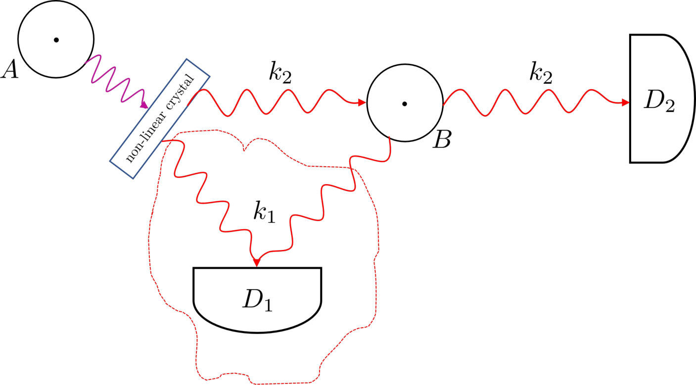
Refer to caption
Figure 6: Systems AA and BB describe 22-level systems, respectively. The allowed interactions are infinitesimally described as follows: If AA is in its excited state, it can emit a photon. Through parametric down-conversion, the photon is converted into two photons (of lower energy). One of those two photons, k1k_{1}, is sent to a detector D1D_{1}. The other, k2k_{2}, is sent to BB. If BB is in its ground state, it absorbs k2k_{2}. If BB is in its excited state, it cannot absorb k2k_{2}, so k2k_{2} passes through BB and travels to a detector D2D_{2}. Additionally, in this case, BB can emit a photon, indistinguishable from k1k_{1}, to D1D_{1}.
Example.

We consider the scenario of two 22-level atoms that can interact according to the processes specified in Fig. 6. We can describe this process either via a dilation (as in Theorem V.6) or via the Kraus operators (as in Corollary V.16). In the dilation picture, we introduce an auxiliary Hilbert space ℋE:=ℋ1⊗ℋ2\mathcal{H}_{E}:=\mathcal{H}_{1}\otimes\mathcal{H}_{2}, where ℋi\mathcal{H}_{i} is for the ithi^{\textrm{th}} photon. Then, the process is described by V=(𝟙A⊗U)​(A⊗𝟙B)+(𝟙A⊗B)V=(\mathds{1}_{A}\otimes U)(A\otimes\mathds{1}_{B})+(\mathds{1}_{A}\otimes B), with

A∈ℬ⁡(ℋA,ℋA⊗ℋE),A\displaystyle A\in\mathcal{B}\left(\mathcal{H}_{A};\mathcal{H}_{A}\otimes\mathcal{H}_{E}\right),~A =|0⟩⟨1|A⊗|11⟩E,\displaystyle=\lvert 0\rangle\langle 1\rvert_{A}\otimes\lvert 11\rangle_{E},
B∈ℬ⁡(ℋB,ℋB⊗ℋE),B\displaystyle B\in\mathcal{B}\left(\mathcal{H}_{B};\mathcal{H}_{B}\otimes\mathcal{H}_{E}\right),~B =|10⟩E⊗|0⟩⟨1|B,\displaystyle=\lvert 10\rangle_{E}\otimes\lvert 0\rangle\langle 1\rvert_{B},
U∈𝒰⁡(ℋE⊗ℋB,ℋB⊗ℋE),U\displaystyle U\in\mathcal{U}(\mathcal{H}_{E}\otimes\mathcal{H}_{B};\mathcal{H}_{B}\otimes\mathcal{H}_{E}),~U =𝔽E;B​(𝟙ℋ1⊗U~),\displaystyle=\mathbb{F}_{E;B}(\mathds{1}_{\mathcal{H}_{1}}\otimes\tilde{U}),

where U~∈𝒰⁡(ℋ2⊗ℋB)\tilde{U}\in\mathcal{U}\left(\mathcal{H}_{2}\otimes\mathcal{H}_{B}\right) is determined by

U~|00⟩ℋ2​B=|00⟩ℋ2​B,U~|10⟩ℋ2​B=|01⟩ℋ2​B,U~|11⟩ℋ2​B=|11⟩ℋ2​B.\displaystyle\tilde{U}\lvert 00\rangle_{\mathcal{H}_{2}B}=\lvert 00\rangle_{\mathcal{H}_{2}B},~\tilde{U}\lvert 10\rangle_{\mathcal{H}_{2}B}=\lvert 01\rangle_{\mathcal{H}_{2}B},~\tilde{U}\lvert 11\rangle_{\mathcal{H}_{2}B}=\lvert 11\rangle_{\mathcal{H}_{2}B}.

The crucial feature of this example is that the CP-part of the generator (trE​[V⋅V†]\mathrm{tr}_{E}\left[V\cdot V^{\dagger}\right]) cannot be written as a convex combination of the two building blocks (Φs​c\Phi_{sc} and idA⊗B^\mathrm{id}_{A}\otimes\hat{B}). As mentioned also in the quantization procedure before, this is a pure quantum feature and stems from the fact that it cannot be determined if a photon arriving at the detector D1D_{1} came from BB or AA. Hence, the system remains in a superposition state.
We can also look at the usual representation via jump operators. This can be achieved by switching from dilations to Kraus operators. We obtain the two jump-operators

L1:=Le⊗La⏟=:ϕ1+𝟙A⊗Le⏟B1,L2:=Le⊗|1⟩⟨1|⏟=:ϕ2,\displaystyle L_{1}:=\underbrace{L_{e}\otimes L_{a}}_{=:\phi_{1}}+\mathds{1}_{A}\otimes\underbrace{L_{e}}_{B_{1}},~L_{2}:=\underbrace{L_{e}\otimes\lvert 1\rangle\langle 1\rvert}_{=:\phi_{2}},

where Le=|0⟩⟨1|L_{e}=\lvert 0\rangle\langle 1\rvert and La=Le†L_{a}=L_{e}^{\dagger} describe emission and absorption of a photon, respectively. Thus, the usual Lindblad equation reads:

d​ρd​t=(Le⊗La+𝟙A⊗Le)​ρ​(Le⊗La+𝟙A⊗Le)+(𝟙A⊗Le)​ρ​(𝟙A⊗Le)−12​{𝟙A⊗Le†​Le+Le†​Le⊗𝟙B,ρ}\displaystyle\frac{d\rho}{dt}=(L_{e}\otimes L_{a}+\mathds{1}_{A}\otimes L_{e})\rho(L_{e}\otimes L_{a}+\mathds{1}_{A}\otimes L_{e})+(\mathds{1}_{A}\otimes L_{e})\rho(\mathds{1}_{A}\otimes L_{e})-\frac{1}{2}\left\{\mathds{1}_{A}\otimes L_{e}^{\dagger}L_{e}+L_{e}^{\dagger}L_{e}\otimes\mathds{1}_{B}\,,\,\rho\right\}

It is also possible and instructive to consider the reduced dynamics on system AA, which can also be described by a Lindblad equation, since BB does not communicate to AA (this is not true otherwise):

d​ρAd​t=Le​ρA​Le†−12​{Le†​Le,ρA},\displaystyle\frac{d\rho_{A}}{dt}=L_{e}\rho_{A}L_{e}^{\dagger}-\frac{1}{2}\left\{L_{e}^{\dagger}L_{e}\,,\,\rho_{A}\right\},

where ρA​(t)=trB​[ρ⁡(t)]\rho_{A}(t)=\mathrm{tr}_{B}\left[\rho(t)\right]. Not surprisingly (given our model), this describes an atom emitting photons.

V.3 Generators of semigroups of quantum superchannels

We finally turn to semigroups of quantum superchannels (on finite-dimensional spaces), that is, a collection of quantum superchannels {S^t}t≥0⊆ℬ⁡(ℬ⁡(ℬ⁡(ℋA),ℬ⁡(ℋB)))\{\hat{S}_{t}\}_{t\geq 0}\subseteq\mathcal{B}(\mathcal{B}(\mathcal{B}(\mathcal{H}_{A});\mathcal{B}(\mathcal{H}_{B}))), such that S^0=id\hat{S}_{0}=\mathrm{id}, S^t+s=S^t​S^s\hat{S}_{t+s}=\hat{S}_{t}\hat{S}_{s} and the map t↦S^tt\mapsto\hat{S}_{t} is continuous (w.r.t. any and thus all of the equivalent norms on the finite-dimensional space ℬ⁡(ℬ⁡(ℬ⁡(ℋA),ℬ⁡(ℋB)))\mathcal{B}(\mathcal{B}(\mathcal{B}(\mathcal{H}_{A});\mathcal{B}(\mathcal{H}_{B})))). To formulate a technically slightly stronger result, we call a map S^∈ℬ⁡(ℬ⁡(ℬ⁡(ℋA),ℬ⁡(ℋB)))\hat{S}\in\mathcal{B}(\mathcal{B}(\mathcal{B}(\mathcal{H}_{A});\mathcal{B}(\mathcal{H}_{B}))) a preselecting supermap if ℭA;B∘S^∘ℭA;B−1\mathfrak{C}_{A;B}\circ\hat{S}\circ\mathfrak{C}^{-1}_{A;B} is a Schrödinger B↛AB\not\to A semicausal CP-map. Theorem V.3 then tells us that a superchannel is a special preselecting supermap. Again, as for semicausal CP-maps, we characterize the generators of semigroups of preselecting supermaps and superchannels in two ways: First, we answer how to determine if a given map L^∈ℬ⁡(ℬ⁡(ℬ⁡(ℋA),ℬ⁡(ℋB)))\hat{L}\in\mathcal{B}(\mathcal{B}(\mathcal{B}(\mathcal{H}_{A});\mathcal{B}(\mathcal{H}_{B}))) is such a generator. Second, we provide a normal form for all generators.

The answer to the first question is really a corollary of Lemma V.5 together with Theorem V.3. To this end, define 𝔏^:=ℭA​B;A​B​(ℭA;B∘L^∘ℭA;B−1)∈ℬ⁡(ℋA1⊗ℋB1⊗ℋA2⊗ℋB2)\hat{\mathfrak{L}}:=\mathfrak{C}_{AB;AB}\left(\mathfrak{C}_{A;B}\circ\hat{L}\circ\mathfrak{C}^{-1}_{A;B}\right)\in\mathcal{B}(\mathcal{H}_{A_{1}}\otimes\mathcal{H}_{B_{1}}\otimes\mathcal{H}_{A_{2}}\otimes\mathcal{H}_{B_{2}}), where we fix some orthonormal bases {|ai⟩}i=1dim⁡(ℋA)\{\lvert a_{i}\rangle\}_{i=1}^{\mathrm{dim}(\mathcal{H}_{A})} and {|bj⟩}j=1dim⁡(ℋB)\{\lvert b_{j}\rangle\}_{j=1}^{\mathrm{dim}(\mathcal{H}_{B})} of ℋA\mathcal{H}_{A} and ℋB\mathcal{H}_{B}, such that ℭA;B\mathfrak{C}_{A;B} is defined w.r.t. {|ai⟩}i=1dim⁡(ℋA)\{\lvert a_{i}\rangle\}_{i=1}^{\mathrm{dim}(\mathcal{H}_{A})} and ℭA​B;A​B\mathfrak{C}_{AB;AB} is defined w.r.t. the product of the two bases. Furthermore, we introduced the spaces ℋA1=ℋA2=ℋA\mathcal{H}_{A_{1}}=\mathcal{H}_{A_{2}}=\mathcal{H}_{A} and ℋB1=ℋB2=ℋA\mathcal{H}_{B_{1}}=\mathcal{H}_{B_{2}}=\mathcal{H}_{A} for notational convenience. Finally, we define P⊥∈ℬ⁡(ℋA1⊗ℋB1⊗ℋA2⊗ℋB2)P^{\bot}\in\mathcal{B}(\mathcal{H}_{A_{1}}\otimes\mathcal{H}_{B_{1}}\otimes\mathcal{H}_{A_{2}}\otimes\mathcal{H}_{B_{2}}) to be the orthogonal projection onto the orthogonal complement of {|Ω⟩}\{\lvert\Omega\rangle\}, where |Ω⟩=∑i,j|ai⟩⊗|bj⟩⊗|ai⟩⊗|bj⟩\lvert\Omega\rangle=\sum_{i,j}\lvert a_{i}\rangle\otimes\lvert b_{j}\rangle\otimes\lvert a_{i}\rangle\otimes\lvert b_{j}\rangle. We then have

Lemma V.17.

A linear map L^∈ℬ⁡(ℬ⁡(ℬ⁡(ℋA),ℬ⁡(ℋB)))\hat{L}\in\mathcal{B}(\mathcal{B}(\mathcal{B}(\mathcal{H}_{A});\mathcal{B}(\mathcal{H}_{B}))) generates a semigroup of quantum superchannels if and only if

  • •

    𝔏^\hat{\mathfrak{L}} is self-adjoint and P⊥​𝔏^​P⊥≥0P^{\bot}\hat{\mathfrak{L}}P^{\bot}\geq 0,

  • •

    (𝔽A1;B1⊗𝟙A2)​trB2​[𝔏^]​(𝔽A1;B1⊗𝟙A2)=𝟙B1⊗𝔏^A(\mathbb{F}_{A_{1};B_{1}}\otimes\mathds{1}_{A_{2}})\mathrm{tr}_{B_{2}}\left[\hat{\mathfrak{L}}\right](\mathbb{F}_{A_{1};B_{1}}\otimes\mathds{1}_{A_{2}})=\mathds{1}_{B_{1}}\otimes\hat{\mathfrak{L}}^{A}, for some (then necessarily self-adjoint) 𝔏^A∈ℬ⁡(ℋA1⊗ℋA2)\hat{\mathfrak{L}}^{A}\in\mathcal{B}(\mathcal{H}_{A_{1}}\otimes\mathcal{H}_{A_{2}}) and

  • •

    trA1​[𝔏^A]=0\mathrm{tr}_{A_{1}}\left[\hat{\mathfrak{L}}^{A}\right]=0.

L^\hat{L} is preselecting if and only if the first two conditions hold.

Proof.

Theorem V.3 tells us that {S^t}t≥0\{\hat{S}_{t}\}_{t\geq 0} forming a semigroup of superchannels is eqiuvalent to St=ℭA;B∘S^t∘ℭA;B−1S_{t}=\mathfrak{C}_{A;B}\circ\hat{S}_{t}\circ\mathfrak{C}_{A;B}^{-1} forming a semigroup of Schrödinger B↛AB\not\to A semicausal CP-maps and that the reduced map StAS_{t}^{A} satisfies StA​(𝟙A)=𝟙AS_{t}^{A}(\mathds{1}_{A})=\mathds{1}_{A}. By Lemma V.5 the semicausal semigroup property is equivalent to the first two conditions in the statement. This proves the claim about preselecting L^\hat{L}.
By differentiation, it follows that StA​(𝟙A)=𝟙AS_{t}^{A}(\mathds{1}_{A})=\mathds{1}_{A} is satisfied if and only if LAL^{A}, the generator of {StA}t≥0\{S_{t}^{A}\}_{t\geq 0}, satisfies LA​(𝟙A)=0L^{A}(\mathds{1}_{A})=0. But since trA1​[𝔏^A]=LA​(𝟙A)\mathrm{tr}_{A_{1}}\left[\hat{\mathfrak{L}}^{A}\right]=L^{A}(\mathds{1}_{A}), the claim follows. ∎

We finally turn to a normal form for generators of semigroups of preselecting supermaps and superchannels:

Theorem V.18.

A linear map L^:ℬ⁡(ℬ⁡(ℋA),ℬ⁡(ℋB))→ℬ⁡(ℬ⁡(ℋA),ℬ⁡(ℋB))\hat{L}:\mathcal{B}(\mathcal{B}(\mathcal{H}_{A});\mathcal{B}(\mathcal{H}_{B}))\rightarrow\mathcal{B}(\mathcal{B}(\mathcal{H}_{A});\mathcal{B}(\mathcal{H}_{B})) generates a semigroup of hyper-preselecting supermaps if and only if there exist a Hilbert space ℋE\mathcal{H}_{E}, a state σ∈ℬ⁡(ℋE)\sigma\in\mathcal{B}(\mathcal{H}_{E}), a unitary U∈𝒰⁡(ℋB⊗ℋE)U\in\mathcal{U}(\mathcal{H}_{B}\otimes\mathcal{H}_{E}), a self-adjoint operator HB∈ℬ⁡(ℋB)H_{B}\in\mathcal{B}(\mathcal{H}_{B}), and arbitrary operators A∈ℬ⁡(ℋA⊗ℋE)A\in\mathcal{B}(\mathcal{H}_{A}\otimes\mathcal{H}_{E}), B∈ℬ⁡(ℋB⊗ℋE)B\in\mathcal{B}(\mathcal{H}_{B}\otimes\mathcal{H}_{E}) and KA∈ℬ⁡(ℋA)K_{A}\in\mathcal{B}(\mathcal{H}_{A}), such that L^\hat{L} acts on T∈ℬ⁡(ℬ⁡(ℋA),ℬ⁡(ℋB))T\in\mathcal{B}(\mathcal{B}(\mathcal{H}_{A});\mathcal{B}(\mathcal{H}_{B})) as L^​(T)=Φ^​(T)−κ^L​(T)−κ^R​(T)\hat{L}(T)=\hat{\Phi}(T)-\hat{\kappa}_{L}(T)-\hat{\kappa}_{R}(T), with

Φ^​(T)​(ρ)=trE​[U⁡(T⊗idE)​(A⁡(ρ⊗σ)​A†)​U†]+trE​[B⁡(T⊗idE)​((ρ⊗σ)​A†)​U†]+trE​[U⁡(T⊗idE)​(A⁡(ρ⊗σ))​B†]+trE​[B⁡(T⊗idE)​((ρ⊗σ))​B†],\displaystyle\begin{split}\hat{\Phi}(T)(\rho)=&\mathrm{tr}_{E}\left[U\;(T\otimes\mathrm{id}_{E})(A(\rho\otimes\sigma)A^{\dagger})\;U^{\dagger}\right]+\mathrm{tr}_{E}\left[B\;(T\otimes\mathrm{id}_{E})((\rho\otimes\sigma)A^{\dagger})\;U^{\dagger}\right]\\ &+\mathrm{tr}_{E}\left[U\;(T\otimes\mathrm{id}_{E})(A(\rho\otimes\sigma))\;B^{\dagger}\right]+\mathrm{tr}_{E}\left[B\;(T\otimes\mathrm{id}_{E})((\rho\otimes\sigma))\;B^{\dagger}\right],\end{split} (17)
κ^L​(T)​(ρ)\displaystyle\hat{\kappa}_{L}(T)(\rho) =trE​[B†​U​(T⊗idE)​(A⁡(ρ⊗σ))]+12​trE​[B†​B​(T⊗idE)​(ρ⊗σ)]+T⁡(KA​ρ)+i​HB​T​(ρ),\displaystyle=\mathrm{tr}_{E}\left[B^{\dagger}U\;(T\otimes\mathrm{id}_{E})(A(\rho\otimes\sigma))\right]+\frac{1}{2}\mathrm{tr}_{E}\left[B^{\dagger}B(T\otimes\mathrm{id}_{E})(\rho\otimes\sigma)\right]\;+T(K_{A}\,\rho)+iH_{B}\,T(\rho), (18a)
κ^R​(T)​(ρ)\displaystyle\hat{\kappa}_{R}(T)(\rho) =trE​[(T⊗idE)​((ρ⊗σ)​A†)​U†​B]+12​trE​[(T⊗idE)​(ρ⊗σ)​B†​B]+T⁡(ρ​KA†)−T⁡(ρ)​i​HB.\displaystyle=\mathrm{tr}_{E}\left[(T\otimes\mathrm{id}_{E})((\rho\otimes\sigma)A^{\dagger})\;U^{\dagger}B\right]+\frac{1}{2}\mathrm{tr}_{E}\left[(T\otimes\mathrm{id}_{E})(\rho\otimes\sigma)B^{\dagger}B\right]\;+T(\rho\,K_{A}^{\dagger})-T(\rho)\,iH_{B}. (18b)

We can choose σ\sigma to be pure and ℋE\mathcal{H}_{E} with dim⁡(ℋE)≤(dA​dB)2\mathrm{dim}(\mathcal{H}_{E})\leq(d_{A}d_{B})^{2}, where dAd_{A} and dBd_{B} are the dimensions of ℋA\mathcal{H}_{A} and ℋB\mathcal{H}_{B}, respectively.
Furthermore, L^\hat{L} generates a semigroup of superchannels if and only if L^\hat{L} generates a semigroup of preselecting supermaps and trσ​[A†​A]=KA+KA†\mathrm{tr}_{\sigma}\left[A^{\dagger}A\right]=K_{A}+K_{A}^{\dagger}. In that case, we can split L^\hat{L} into a dissipative part D^\hat{D} and a ‘Hamiltonian’ part H^\hat{H}, i.e., a part which generates a (semi-)group of invertible superchannels whose inverses are superchannels as well. We have L^​(T)=D^​(T)+H^​(T)\hat{L}(T)=\hat{D}(T)+\hat{H}(T), with

D^​(T)​(ρ)=trE​[D^′​(T)​(ρ)]andH^​(T)​(ρ)=−i⁡[HB,T⁡(ρ)]−i​T​([HA,ρ]),\displaystyle\hat{D}(T)(\rho)=\mathrm{tr}_{E}\left[\hat{D}^{\prime}(T)(\rho)\right]\quad\text{and}\quad\hat{H}(T)(\rho)=-i\left[H_{B}\,,\,T(\rho)\right]-iT(\left[H_{A}\,,\,\rho\right]),

where HAH_{A} is the imaginary part of KAK_{A}, where

D^′​(T)​(ρ)\displaystyle\hat{D}^{\prime}(T)(\rho) =U⁡(T⊗idE)​(A⁡(ρ⊗σ)​A†)​U†\displaystyle=U(T\otimes\mathrm{id}_{E})(A(\rho\otimes\sigma)A^{\dagger})U^{\dagger} −12​(T⊗idE)​({A†​A,ρ⊗σ})\displaystyle-\frac{1}{2}(T\otimes\mathrm{id}_{E})(\left\{A^{\dagger}A\,,\,\rho\otimes\sigma\right\}) (19a)
+B⁡(T⊗idE)​(ρ⊗σ)​B†\displaystyle+B(T\otimes\mathrm{id}_{E})(\rho\otimes\sigma)B^{\dagger} −12​{B†​B,(T⊗idE)​(ρ⊗σ)}\displaystyle-\frac{1}{2}\left\{B^{\dagger}B\,,\,(T\otimes\mathrm{id}_{E})(\rho\otimes\sigma)\right\} (19b)
+[U⁡(T⊗idE)​(A⁡(ρ⊗σ)),B†]\displaystyle+\left[U(T\otimes\mathrm{id}_{E})(A(\rho\otimes\sigma))\,,\,B^{\dagger}\right] +[B,(T⊗idE)​((ρ⊗σ)​A†)​U†],\displaystyle+\left[B\,,\,(T\otimes\mathrm{id}_{E})((\rho\otimes\sigma)A^{\dagger})U^{\dagger}\right], (19c)

and where [⋅,⋅][\cdot,\cdot] and {⋅,⋅}\{\cdot,\cdot\} denote the commutator and anticommutator, respectively.

Remark V.19.

Similarly to Theorem V.6, the proof of Theorem V.18 is constructive. In Appendix D we discuss in detail how to obtain the operators AA, UU, KAK_{A}, BB, HAH_{A} and HBH_{B} starting from the conditions in Theorem V.17.

As in the classical case, the proof strategy is to use the relation between superchannels and semicausal channels and Theorem V.6. As this translation process is more involved than in the classical case, we need two auxilliary lemmas.

Lemma V.20.

Let S:ℬ⁡(ℋA⊗ℋB)→ℬ⁡(ℋA⊗ℋB)S:\mathcal{B}(\mathcal{H}_{A}\otimes\mathcal{H}_{B})\rightarrow\mathcal{B}(\mathcal{H}_{A}\otimes\mathcal{H}_{B}) be given by

S⁡(X)=trE​[(𝟙A⊗LB)​(LA⊗𝟙B)​X​(RA†⊗𝟙B)​(𝟙A⊗RB†)],\displaystyle S(X)=\mathrm{tr}_{E}\left[(\mathds{1}_{A}\otimes L_{B})(L_{A}\otimes\mathds{1}_{B})X(R_{A}^{\dagger}\otimes\mathds{1}_{B})(\mathds{1}_{A}\otimes R_{B}^{\dagger})\right], (20)

with Hilbert spaces ℋC\mathcal{H}_{C} and ℋE\mathcal{H}_{E}, operators LA,RA∈ℬ⁡(ℋA,ℋA⊗ℋC)L_{A},R_{A}\in\mathcal{B}(\mathcal{H}_{A};\mathcal{H}_{A}\otimes\mathcal{H}_{C}) and LB,RB∈ℬ⁡(ℋC⊗ℋB,ℋB⊗ℋE)L_{B},R_{B}\in\mathcal{B}(\mathcal{H}_{C}\otimes\mathcal{H}_{B};\mathcal{H}_{B}\otimes\mathcal{H}_{E}). Then, for T∈ℬ⁡(ℬ⁡(ℋA),ℬ⁡(ℋB))T\in\mathcal{B}(\mathcal{B}(\mathcal{H}_{A});\mathcal{B}(\mathcal{H}_{B})) and ρ∈ℬ⁡(ℋA)\rho\in\mathcal{B}(\mathcal{H}_{A}),

[ℭA;B−1∘S∘ℭA;B]​(T)​(ρ)=trE​[VL​(T⊗idC)​(WL​ρ​WR†)​VR†],\displaystyle\left[\mathfrak{C}_{A;B}^{-1}\circ S\circ\mathfrak{C}_{A;B}\right](T)(\rho)=\mathrm{tr}_{E}\left[V_{L}(T\otimes\mathrm{id}_{C})\left(W_{L}\rho W_{R}^{\dagger}\right)V_{R}^{\dagger}\right], (21)

with VL=LB​𝔽B;CV_{L}=L_{B}\mathbb{F}_{B;C}, VR=RB​𝔽B;CV_{R}=R_{B}\mathbb{F}_{B;C}; and WL=LATAW_{L}=L_{A}^{T_{A}}, WR=RATAW_{R}=R_{A}^{T_{A}}. Here, the partial transpose on ℋA\mathcal{H}_{A} is taken w.r.t. the basis used to define the Choi–Jamiołkowski isomorphism.

Proof.

The proof is a direct calculation. We present it in detail in Appendix A. ∎

Lemma V.21.

Let X∈ℬ⁡(ℋA⊗ℋC,ℋA⊗ℋB)X\in\mathcal{B}(\mathcal{H}_{A}\otimes\mathcal{H}_{C};\mathcal{H}_{A}\otimes\mathcal{H}_{B}), Y∈ℬ⁡(ℋA⊗ℋB,ℋA⊗ℋC)Y\in\mathcal{B}(\mathcal{H}_{A}\otimes\mathcal{H}_{B};\mathcal{H}_{A}\otimes\mathcal{H}_{C}), ρ∈𝒮1​(ℋB)\rho\in\mathcal{S}_{1}(\mathcal{H}_{B}). Then trρ​[X​Y]T=trC​[YTA​(𝟙A⊗ρ)​XTA]\mathrm{tr}_{\rho}\left[XY\right]^{T}=\mathrm{tr}_{C}\left[Y^{T_{A}}(\mathds{1}_{A}\otimes\rho)X^{T_{A}}\right].

Proof.

The proof is a direct calculation. We present it in detail in Appendix A. ∎

We are finally ready to prove Theorem V.18

Proof.

(Theorem V.18) The idea is to relate the generators of superchannels to semicausal maps. This relation is given by definition for preselecting superamps and by Theorem V.3 for superchannels. For a generator L^\hat{L} of a semigroup of preselecting supermaps {St^}t≥0\{\hat{S_{t}}\}_{t\geq 0}, we have

L^=ℭA;B−1∘dd​t|t=0​[ℭA;B∘S^t∘ℭA;B−1]∘ℭA;B.\displaystyle\hat{L}=\mathfrak{C}_{A;B}^{-1}\circ\frac{d}{dt}\bigg|_{t=0}[\mathfrak{C}_{A;B}\circ\hat{S}_{t}\circ\mathfrak{C}_{A;B}^{-1}]\circ\mathfrak{C}_{A;B}.

Thus L^\hat{L} generates a semigroup of preselecting supermaps if and only if L^\hat{L} can be written as L^=ℭA;B−1∘L∘ℭA;B\hat{L}=\mathfrak{C}_{A;B}^{-1}\circ L\circ\mathfrak{C}_{A;B} for some generator LL of a semigroup of Schrödinger B↛AB\not\to A semicausal CP-maps. Thus to prove the first part of our theorem, we can take the normal form in Corollary V.15 and compute the similarity transformation above. We now execute this in detail. To start with, Corollary V.15 tells us that L⁡(ρ)=ΦS​(ρ)−K​ρ−ρ​K†L(\rho)=\Phi_{S}(\rho)-K\rho-\rho K^{\dagger}, where

ΦS​(ρ)\displaystyle\Phi_{S}(\rho) =trE​[V​ρ​V†], with ​V=(𝟙A⊗U~)​(A~⊗𝟙B)+(𝟙A⊗B~),\displaystyle=\mathrm{tr}_{E}\left[V\rho V^{\dagger}\right],\text{ with }V=(\mathds{1}_{A}\otimes\tilde{U})(\tilde{A}\otimes\mathds{1}_{B})+(\mathds{1}_{A}\otimes\tilde{B}), (22a)
K\displaystyle K =(𝟙A⊗B~†​U~)​(A~⊗𝟙B)+12​𝟙A⊗B~†​B~+K~A⊗𝟙B+𝟙A⊗i​H~B.\displaystyle=(\mathds{1}_{A}\otimes\tilde{B}^{\dagger}\tilde{U})(\tilde{A}\otimes\mathds{1}_{B})+\frac{1}{2}\mathds{1}_{A}\otimes\tilde{B}^{\dagger}\tilde{B}+\tilde{K}_{A}\otimes\mathds{1}_{B}+\mathds{1}_{A}\otimes i\tilde{H}_{B}. (22b)

for some unitary U~∈𝒰⁡(ℋE⊗ℋB,ℋB⊗ℋE)\tilde{U}\in\mathcal{U}(\mathcal{H}_{E}\otimes\mathcal{H}_{B};\mathcal{H}_{B}\otimes\mathcal{H}_{E}), some self-adjoint H~B∈ℬ⁡(ℋB)\tilde{H}_{B}\in\mathcal{B}(\mathcal{H}_{B}) and some operators A~∈ℬ⁡(ℋA,ℋA⊗ℋE)\tilde{A}\in\mathcal{B}(\mathcal{H}_{A};\mathcal{H}_{A}\otimes\mathcal{H}_{E}), B~∈ℬ⁡(ℋB,ℋB⊗ℋE)\tilde{B}\in\mathcal{B}(\mathcal{H}_{B};\mathcal{H}_{B}\otimes\mathcal{H}_{E}) and K~A∈ℬ⁡(ℋA)\tilde{K}_{A}\in\mathcal{B}(\mathcal{H}_{A}). In order to apply Lemma V.20, we fix a unit vector |ξ⟩∈ℋE\lvert\xi\rangle\in\mathcal{H}_{E} and define ΞA:=𝟙A⊗|ξ⟩∈ℬ(ℋA;ℋA⊗ℋE)\Xi_{A}:=\mathds{1}_{A}\otimes\lvert\xi\rangle\in\mathcal{B}(\mathcal{H}_{A};\mathcal{H}_{A}\otimes\mathcal{H}_{E}) and ΞB:=|ξ⟩⊗𝟙B∈ℬ(ℋB;ℋE⊗ℋB)\Xi_{B}:=\lvert\xi\rangle\otimes\mathds{1}_{B}\in\mathcal{B}(\mathcal{H}_{B};\mathcal{H}_{E}\otimes\mathcal{H}_{B}), so that 𝟙A⊗B~=(𝟙A⊗B~​ΞB†)​(ΞA⊗𝟙B)\mathds{1}_{A}\otimes\tilde{B}=(\mathds{1}_{A}\otimes\tilde{B}\Xi_{B}^{\dagger})(\Xi_{A}\otimes\mathds{1}_{B}). We can then write

ΦS​(ρ)\displaystyle\Phi_{S}(\rho) =trE​[(𝟙A⊗U~)​(A~⊗𝟙B)​ρ​(A~†⊗𝟙B)​(𝟙A⊗U†)]+trE​[(𝟙A⊗B~​ΞB†)​(ΞA⊗𝟙B)​ρ​(ΞA†⊗𝟙B)​(𝟙A⊗ΞB​B~†)]\displaystyle=\mathrm{tr}_{E}\left[(\mathds{1}_{A}\otimes\tilde{U})(\tilde{A}\otimes\mathds{1}_{B})\rho(\tilde{A}^{\dagger}\otimes\mathds{1}_{B})(\mathds{1}_{A}\otimes U^{\dagger})\right]+\mathrm{tr}_{E}\left[(\mathds{1}_{A}\otimes\tilde{B}\Xi_{B}^{\dagger})(\Xi_{A}\otimes\mathds{1}_{B})\rho(\Xi_{A}^{\dagger}\otimes\mathds{1}_{B})(\mathds{1}_{A}\otimes\Xi_{B}\tilde{B}^{\dagger})\right]
+trE​[(𝟙A⊗U~)​(A~⊗𝟙B)​ρ​(ΞA†⊗𝟙B)​(𝟙A⊗ΞB​B~†)]+trE​[(𝟙A⊗B~​ΞB†)​(ΞA⊗𝟙B)​ρ​(A~†⊗𝟙B)​(𝟙A⊗U†)],\displaystyle+\mathrm{tr}_{E}\left[(\mathds{1}_{A}\otimes\tilde{U})(\tilde{A}\otimes\mathds{1}_{B})\rho(\Xi_{A}^{\dagger}\otimes\mathds{1}_{B})(\mathds{1}_{A}\otimes\Xi_{B}\tilde{B}^{\dagger})\right]+\mathrm{tr}_{E}\left[(\mathds{1}_{A}\otimes\tilde{B}\Xi_{B}^{\dagger})(\Xi_{A}\otimes\mathds{1}_{B})\rho(\tilde{A}^{\dagger}\otimes\mathds{1}_{B})(\mathds{1}_{A}\otimes U^{\dagger})\right],

which is an expression suitable for a term by term application of Lemma V.20. Doing so yields

Φ^​(T)​(ρ)\displaystyle\hat{\Phi}(T)(\rho) :=(ℭA;B−1∘ΦS∘ℭA;B)​(T)​(ρ)\displaystyle:=(\mathfrak{C}^{-1}_{A;B}\circ\Phi_{S}\circ\mathfrak{C}_{A;B})(T)(\rho)
=trE​[U⁡(T⊗idE)​(A⁡(ρ⊗σ)​A†)​U†]+trE​[B⁡(T⊗idE)​((ρ⊗σ)​A†)​U†]\displaystyle=\mathrm{tr}_{E}\left[U\;(T\otimes\mathrm{id}_{E})(A(\rho\otimes\sigma)A^{\dagger})\;U^{\dagger}\right]+\mathrm{tr}_{E}\left[B\;(T\otimes\mathrm{id}_{E})((\rho\otimes\sigma)A^{\dagger})\;U^{\dagger}\right]
+trE​[U⁡(T⊗idE)​(A⁡(ρ⊗σ))​B†]+trE​[B⁡(T⊗idE)​((ρ⊗σ))​B†],\displaystyle+\mathrm{tr}_{E}\left[U\;(T\otimes\mathrm{id}_{E})(A(\rho\otimes\sigma))\;B^{\dagger}\right]+\mathrm{tr}_{E}\left[B\;(T\otimes\mathrm{id}_{E})((\rho\otimes\sigma))\;B^{\dagger}\right],

where we defined U:=U~​𝔽B;EU:=\tilde{U}\mathbb{F}_{B;E}, B:=B~​ΞB†​𝔽B;EB:=\tilde{B}\Xi_{B}^{\dagger}\mathbb{F}_{B;E}, A:=A~TA​ΞA†A:=\tilde{A}^{T_{A}}\Xi_{A}^{\dagger} and σ:=|ξ⟩⟨ξ|\sigma:=\lvert\xi\rangle\langle\xi\rvert. This proves Equation (17). Similarly, upon defining κL​(ρ):=K​ρ\kappa_{L}(\rho):=K\rho we can write 22 2 The partial trace trℂ​[⋅]\mathrm{tr}_{\mathbb{C}}\left[\cdot\right] over the one-dimensional space ℂ\mathbb{C} is just to ensure formal similarity with Lemma V.20.

κL​(ρ)\displaystyle\kappa_{L}(\rho) =trE​[(𝟙A⊗𝔽E;B​ΞB​B~†​U~)​(A~⊗𝟙B)​ρ​(ΞA†⊗𝟙B)​(𝟙A⊗𝔽B;E)]+trE​[(𝟙A⊗𝔽E;B​ΞB​B~†​B~​ΞB†)​(ΞA⊗𝟙B)​ρ​(ΞA†⊗𝟙B)​(𝟙A⊗𝔽B;E)]\displaystyle=\mathrm{tr}_{E}\left[(\mathds{1}_{A}\otimes\mathbb{F}_{E;B}\Xi_{B}\tilde{B}^{\dagger}\tilde{U})(\tilde{A}\otimes\mathds{1}_{B})\rho(\Xi_{A}^{\dagger}\otimes\mathds{1}_{B})(\mathds{1}_{A}\otimes\mathbb{F}_{B;E})\right]+\mathrm{tr}_{E}\left[(\mathds{1}_{A}\otimes\mathbb{F}_{E;B}\Xi_{B}\tilde{B}^{\dagger}\tilde{B}\Xi_{B}^{\dagger})(\Xi_{A}\otimes\mathds{1}_{B})\rho(\Xi_{A}^{\dagger}\otimes\mathds{1}_{B})(\mathds{1}_{A}\otimes\mathbb{F}_{B;E})\right]
+trℂ​[(𝟙A⊗𝟙B)​(K~A⊗𝟙B)​ρ​(𝟙A⊗𝟙B)​(𝟙A⊗𝟙B)]+trℂ​[(𝟙A⊗i​HB)​(𝟙A⊗𝟙B)​ρ​(𝟙A⊗𝟙B)​(𝟙A⊗𝟙B)],\displaystyle+\mathrm{tr}_{\mathbb{C}}\left[(\mathds{1}_{A}\otimes\mathds{1}_{B})(\tilde{K}_{A}\otimes\mathds{1}_{B})\rho(\mathds{1}_{A}\otimes\mathds{1}_{B})(\mathds{1}_{A}\otimes\mathds{1}_{B})\right]+\mathrm{tr}_{\mathbb{C}}\left[(\mathds{1}_{A}\otimes iH_{B})(\mathds{1}_{A}\otimes\mathds{1}_{B})\rho(\mathds{1}_{A}\otimes\mathds{1}_{B})(\mathds{1}_{A}\otimes\mathds{1}_{B})\right],

and apply Lemma V.20 term by term, which yields

κ^L​(T)​(ρ)\displaystyle\hat{\kappa}_{L}(T)(\rho) :=(ℭA;B−1∘κL∘ℭA;B)​(T)​(ρ)\displaystyle:=(\mathfrak{C}^{-1}_{A;B}\circ\kappa_{L}\circ\mathfrak{C}_{A;B})(T)(\rho)
=trE​[B†​U​(T⊗idE)​(A⁡(ρ⊗σ))]+12​trE​[B†​B​(T⊗idE)​(ρ⊗σ)]+T⁡(KA​ρ)+i​HB​T​(ρ),\displaystyle=\mathrm{tr}_{E}\left[B^{\dagger}U\;(T\otimes\mathrm{id}_{E})(A(\rho\otimes\sigma))\right]+\frac{1}{2}\mathrm{tr}_{E}\left[B^{\dagger}B(T\otimes\mathrm{id}_{E})(\rho\otimes\sigma)\right]\;+T(K_{A}\,\rho)+iH_{B}\,T(\rho),

where UU, AA and BB are defined as above and KA:=(K~A)TK_{A}:=(\tilde{K}_{A})^{T} and HB:=H~BH_{B}:=\tilde{H}_{B}. An analogous calculation with κR​(ρ):=ρ​K†\kappa_{R}(\rho):=\rho K^{\dagger} and κ^R​(T):=(ℭA;B−1∘κR∘ℭA;B)​(T)\hat{\kappa}_{R}(T):=(\mathfrak{C}^{-1}_{A;B}\circ\kappa_{R}\circ\mathfrak{C}_{A;B})(T) finishes the proof of the first part, since the claim about the dimension of ℋE\mathcal{H}_{E} follows form the corresponding statements in Theorem V.6.

To prove the second part, first remember that we have observed above that Theorem V.3 implies that LL is Schrödinger B↛AB\not\to A semicausal, with trB​[L⁡(ρ)]=LA​(trB​[ρ])\mathrm{tr}_{B}\left[L(\rho)\right]=L^{A}(\mathrm{tr}_{B}\left[\rho\right]). Furthermore, if we write St=ℭA;B∘S^t∘ℭA;B−1S_{t}=\mathfrak{C}_{A;B}\circ\hat{S}_{t}\circ\mathfrak{C}^{-1}_{A;B}, then Theorem V.3 implies that StS_{t} is Schrödinger B↛AB\not\to A semicausal for all t≥0t\geq 0, with trB​[St​(ρ)]=StA​(trB​[ρ])\mathrm{tr}_{B}\left[S_{t}(\rho)\right]=S_{t}^{A}(\mathrm{tr}_{B}\left[\rho\right]) and also StA​(𝟙A)=𝟙AS_{t}^{A}(\mathds{1}_{A})=\mathds{1}_{A} holds. Differentiating that expression at t=0t=0 yields the equivalent condition LA​(𝟙A)=0L^{A}(\mathds{1}_{A})=0. So, our goal is to incorporate the last condition into the form of (22). To do so, we determine LAL^{A} by calculating trB​[L​(ρ)]\mathrm{tr}_{B}\left[L(\rho)\right], where LL is in the form of (22). We obtain trB​[L⁡(ρ)]=trE​[A~​trB​[ρ]​A~†]−K~A​trB​[ρ]−trB​[ρ]​K~A†\mathrm{tr}_{B}\left[L(\rho)\right]=\mathrm{tr}_{E}\left[\tilde{A}\,\mathrm{tr}_{B}\left[\rho\right]\,\tilde{A}^{\dagger}\right]-\tilde{K}_{A}\mathrm{tr}_{B}\left[\rho\right]-\mathrm{tr}_{B}\left[\rho\right]\tilde{K}_{A}^{\dagger}. Thus, the condition LA​(𝟙)=0L^{A}(\mathds{1})=0 holds if and only if trE​[A~​A~†]=K~A+K~A†\mathrm{tr}_{E}\left[\tilde{A}\tilde{A}^{\dagger}\right]=\tilde{K}_{A}+\tilde{K}_{A}^{\dagger}. Transposing both sides of this equation and using that the definition of AA implies that A~=ATA​ΞA\tilde{A}=A^{T_{A}}\Xi_{A}, yields (trE​[ATA​(𝟙A⊗σ)​(A†)TA])T=KA+KA†\left(\mathrm{tr}_{E}\left[A^{T_{A}}(\mathds{1}_{A}\otimes\sigma)(A^{\dagger})^{T_{A}}\right]\right)^{T}=K_{A}+K_{A}^{\dagger}. But the left hand side is, by Lemma V.21, equal to trσ​[A†​A]\mathrm{tr}_{\sigma}\left[A^{\dagger}A\right]. This proves the claim that L^\hat{L} generates a semigroup of superchannels if and only if L^\hat{L} is hyper-preselecting and trσ​[A†​A]=KA+KA†\mathrm{tr}_{\sigma}\left[A^{\dagger}A\right]=K_{A}+K_{A}^{\dagger}. Finally, defining HA:=12​i​(KA−KA†)H_{A}:=\frac{1}{2i}(K_{A}-K_{A}^{\dagger}) and a few rearrangements lead to (19).
∎

VI Conclusion

Summary

The underlying question of this work was: How can we mathematically characterize the processes that describe the aging of quantum devices? We have argued that, under a Markovianity assumption, such processes can be modeled by continuous semigroups of quantum superchannels. Therefore, the goal of this work was to provide a full characterization of such semigroups of superchannels.

We have derived such a general characterization in terms of the generators of these semigroups. Crucially, we have exploited that superchannels correspond to certain semicausal maps, and that therefore it suffices to characterize generators of semigroups of semicausal maps. We have demonstrated both an efficient procedure for checking whether a given generator is indeed a valid semicausal GKLS generator and a complete characterization of such valid semicausal GKLS generators. The latter is constructive in the sense that it can be used to describe parametrizations of these generators. Aside from the theoretical relevance of these results, they will be valuable in studying properties of these generators numerically. Finally, we have translated these results back to the level of superchannels, thus answering our initial question.

We have also posed and answered the classical counterpart of the above question. I.e., we have characterized the generators semigroups of classical superchannels and of semicausal non-negative maps. These results for the classical case might be of independent interest. From the perspective of quantum information theory, they provide a comparison helpful to understand and interpret the characterizations in the quantum case.

Outlook and open questions

We conclude by presenting some open questions raised by our work. First, in our proof of the characterization of semicausal GKLS generators, we have described a procedure for constructing a semicausal CP-map associated to such a generator. We believe that this method can be applied to a wide range of problems. Determining the exact scope of this method is currently work in progress.

Second, there is a wealth of results on the spectral properties of quantum channels and, in particular, semigroups of quantum channels. With the explicit form of generators of semigroups of superchannels now known, we can conduct analogous studies for semigroups of quantum superchannels. Understanding such spectral properties, and potentially how they differ from the properties in the scenario of quantum channels, would in particular lead to a better understanding of the asymptotic behavior of semigroups of superchannels, e.g., w.r.t. entropy production Gour and Wilde 2021; Gour 2019, the thermodynamics of quantum channels Faist et al. 2019 or entanglement-breaking properties Chen and Chitambar 2020.

A further natural question would be a quantum superchannel analogue of the Markovianity problem: When can a quantum superchannel S^\hat{S} be written as eL^e^{\hat{L}} for some L^\hat{L} that generates a semigroup of superchannels? Several works have investigated the Markovianity problem for quantum channels Wolf et al. 2008; Cubitt et al. 2012a; Cubitt et al. 2012b; Onorati et al. 2021 and a divisibility variant of this question, both for quantum channels and for stochastic matrices Wolf and Cirac 2008; Bausch and Cubitt 2016; Caro and Graswald 2021. It would be interesting to see how these results translate to quantum or classical superchannels. Similarly, we can now ask questions of reachability along Markovian paths. Yet another question aiming at understanding Markovianity: If we consider master equations arising from a Markovianity assumption on the underlying process formalized not via semigroups of channels, but instead via semigroups of superchannels, what are the associated classes of (time-dependent) generators and corresponding CPTP evolutions?

Two related directions, both of which will lead to a better understanding of Markovian structures in higher order quantum operations, are: Support our mathematical characterization of the generators of semigroups of superchannels by a physical interpretation, similar to the Monte Carlo wave function interpretation of Lindblad generators of quantum channels. And extend our characterization from superchannels to general higher order maps.

This work has focused on generators of general semigroups of superchannels, without further restrictions. For quantum channels and their Lindblad generators, there exists a well developed theory of locality, at the center of which are Lieb-Robinson bounds Nachtergaele et al. 2019. If we put locality restrictions on generators of superchannels, how do these translate to the generated superchannels?

Finally, an important conceptual direction for future work is to identify further applications of our theory of dynamical semigroups of superchannels. In the introduction we gave a physical meaning to semigroups of superchannels by relating them to the decay process of quantum devices. This, however, is only one possible interpretation. For example, semigroups of superchannels might also describe a manufacturing process, where a quantum device is created layer-by-layer. We hope that other use-cases will be found in the future.

Acknowledgments

Both M.C.C. and M.H. thank Michael M. Wolf for insightful discussions about the contents of this paper. We also thank Li Gao, Lisa Hänggli, Robert König, and Farzin Salek for helpful suggestions for improving the presentation. Also, M.C.C. and M.H. thank the anonymous reviewers from TQC 2022 and from the Journal of Mathematical Physics for their constructive criticism. M.H. was supported by the Bavarian excellence network ENB via the International PhD Programme of Excellence Exploring Quantum Matter (EXQM). M.C.C. gratefully acknowledges support from the TopMath Graduate Center of the TUM Graduate School at the Technische Universität München, Germany, from the TopMath Program at the Elite Network of Bavaria, and from the German Academic Scholarship Foundation (Studienstiftung des deutschen Volkes).

Appendix A Proof of Lemmas V.20 and V.21

In this appendix we provide a complete proof of Lemmas V.20 and V.21.

Lemma A.1.

(Restatement of Lemma V.20) Let S:ℬ⁡(ℋA⊗ℋB)→ℬ⁡(ℋA⊗ℋB)S:\mathcal{B}(\mathcal{H}_{A}\otimes\mathcal{H}_{B})\rightarrow\mathcal{B}(\mathcal{H}_{A}\otimes\mathcal{H}_{B}) be given by

S⁡(X)=trE​[(𝟙A⊗LB)​(LA⊗𝟙B)​X​(RA†⊗𝟙B)​(𝟙A⊗RB†)],\displaystyle S(X)=\mathrm{tr}_{E}\left[(\mathds{1}_{A}\otimes L_{B})(L_{A}\otimes\mathds{1}_{B})X(R_{A}^{\dagger}\otimes\mathds{1}_{B})(\mathds{1}_{A}\otimes R_{B}^{\dagger})\right],

with Hilbert spaces ℋC\mathcal{H}_{C} and ℋE\mathcal{H}_{E}, operators LA,RA∈ℬ⁡(ℋA,ℋA⊗ℋC)L_{A},R_{A}\in\mathcal{B}(\mathcal{H}_{A};\mathcal{H}_{A}\otimes\mathcal{H}_{C}) and LB,RB∈ℬ⁡(ℋC⊗ℋB,ℋB⊗ℋE)L_{B},R_{B}\in\mathcal{B}(\mathcal{H}_{C}\otimes\mathcal{H}_{B};\mathcal{H}_{B}\otimes\mathcal{H}_{E}). Then, for T∈ℬ⁡(ℬ⁡(ℋA),ℬ⁡(ℋB))T\in\mathcal{B}(\mathcal{B}(\mathcal{H}_{A});\mathcal{B}(\mathcal{H}_{B})) and ρ∈ℬ⁡(ℋA)\rho\in\mathcal{B}(\mathcal{H}_{A}),

[ℭA;B−1∘S∘ℭA;B]​(T)​(ρ)=trE​[VL​(T⊗idC)​(WL​ρ​WR†)​VR†],\displaystyle\left[\mathfrak{C}_{A;B}^{-1}\circ S\circ\mathfrak{C}_{A;B}\right](T)(\rho)=\mathrm{tr}_{E}\left[V_{L}(T\otimes\mathrm{id}_{C})\left(W_{L}\rho W_{R}^{\dagger}\right)V_{R}^{\dagger}\right],

with VL=LB​𝔽B;CV_{L}=L_{B}\mathbb{F}_{B;C}, VR=RB​𝔽B;CV_{R}=R_{B}\mathbb{F}_{B;C}; and WL=LATAW_{L}=L_{A}^{T_{A}}, WR=RATAW_{R}=R_{A}^{T_{A}}. Here, the partial transpose on ℋA\mathcal{H}_{A} is taken w.r.t. the basis used to define the Choi–Jamiołkowski isomorphism.

Proof.

Let {|ei⟩}i\{\lvert e_{i}\rangle\}_{i} be the orthonormal basis of ℋA\mathcal{H}_{A}, w.r.t. which the Choi–Jamiołkowski isomorphism is defined. Let {|cn⟩}n\{\lvert c_{n}\rangle\}_{n} be an orthonormal basis of ℋC\mathcal{H}_{C}. Then the formal calculation, which is an algebraic version of drawing the corresponding tensor-network pictures, can be executed as follows:

[ℭA;B−1∘S∘ℭA;B]​(T)​(ρ)\displaystyle\left[\mathfrak{C}_{A;B}^{-1}\circ S\circ\mathfrak{C}_{A;B}\right](T)(\rho) =trA​[(ρT⊗𝟙B)​trE​[(𝟙A⊗LB)​(LA⊗𝟙B)​ℭA;B​(T)​(RA†⊗𝟙B)​(𝟙A⊗RB†)]]\displaystyle=\mathrm{tr}_{A}\left[(\rho^{T}\otimes\mathds{1}_{B})\,\mathrm{tr}_{E}\left[(\mathds{1}_{A}\otimes L_{B})(L_{A}\otimes\mathds{1}_{B})\mathfrak{C}_{A;B}(T)(R_{A}^{\dagger}\otimes\mathds{1}_{B})(\mathds{1}_{A}\otimes R_{B}^{\dagger})\right]\right]
=trE​[LB​trA​[(ρT⊗𝟙C⊗𝟙B)​(LA⊗𝟙B)​ℭA;B​(T)​(RA†⊗𝟙B)]​RB†]\displaystyle=\mathrm{tr}_{E}\left[L_{B}\,\mathrm{tr}_{A}\left[(\rho^{T}\otimes\mathds{1}_{C}\otimes\mathds{1}_{B})(L_{A}\otimes\mathds{1}_{B})\mathfrak{C}_{A;B}(T)(R_{A}^{\dagger}\otimes\mathds{1}_{B})\right]R_{B}^{\dagger}\right]
=∑i,jtrE[LB(trA[(ρT⊗𝟙C)LA|ei⟩⟨ej|RA†]⊗T(|ei⟩⟨ej|)RB†]\displaystyle=\sum_{i,j}\mathrm{tr}_{E}\left[L_{B}\,\left(\mathrm{tr}_{A}\left[(\rho^{T}\otimes\mathds{1}_{C})L_{A}\lvert e_{i}\rangle\langle e_{j}\rvert R_{A}^{\dagger}\right]\otimes T(\lvert e_{i}\rangle\langle e_{j}\rvert\right)R_{B}^{\dagger}\right]
=∑i,j,k,m,n⟨ekcn|((ρT⊗𝟙C)LA|ei⟩⟨ej|RA†)ekcm⟩trE[LB(|cn⟩⟨cm|⊗T(|ei⟩⟨ej|))RB†]\displaystyle=\sum_{i,j,k,m,n}\langle e_{k}\,c_{n}|\left((\rho^{T}\otimes\mathds{1}_{C})L_{A}\lvert e_{i}\rangle\langle e_{j}\rvert R_{A}^{\dagger}\right)\,e_{k}\,c_{m}\rangle\;\mathrm{tr}_{E}\left[L_{B}\,\left(\lvert c_{n}\rangle\langle c_{m}\rvert\otimes T(\lvert e_{i}\rangle\langle e_{j}\rvert)\right)R_{B}^{\dagger}\right]
=∑i,j,m,n⟨ei|(LAT(ρ⊗|cn⟩⟨cm|)R¯A)ej⟩trE[LB(|cn⟩⟨cm|⊗T(|ei⟩⟨ej|))RB†]\displaystyle=\sum_{i,j,m,n}\langle e_{i}|\left(L_{A}^{T}(\rho\otimes\lvert c_{n}\rangle\langle c_{m}\rvert)\overline{R}_{A}\right)\,e_{j}\rangle\;\mathrm{tr}_{E}\left[L_{B}\,\left(\lvert c_{n}\rangle\langle c_{m}\rvert\otimes T(\lvert e_{i}\rangle\langle e_{j}\rvert)\right)R_{B}^{\dagger}\right]
=∑m,ntrE[LB(|cn⟩⟨cm|⊗T(LAT(ρ⊗|cn⟩⟨cm|)R¯A))RB†]\displaystyle=\sum_{m,n}\mathrm{tr}_{E}\left[L_{B}\,\left(\lvert c_{n}\rangle\langle c_{m}\rvert\otimes T\left(L_{A}^{T}(\rho\otimes\lvert c_{n}\rangle\langle c_{m}\rvert)\overline{R}_{A}\right)\right)R_{B}^{\dagger}\right]
=trE[LB𝔽B;C(T⊗idC)([∑n(𝟙A⊗|cn⟩)LAT(𝟙A⊗|cn⟩)]ρ[∑m(𝟙A⊗|cm⟩)RAT(𝟙A⊗|cm⟩)]†)𝔽B;CRB†]\displaystyle=\mathrm{tr}_{E}\left[L_{B}\mathbb{F}_{B;C}(T\otimes\mathrm{id}_{C})\left(\left[\sum_{n}(\mathds{1}_{A}\otimes\lvert c_{n}\rangle)L_{A}^{T}(\mathds{1}_{A}\otimes\lvert c_{n}\rangle)\right]\,\rho\,\left[\sum_{m}(\mathds{1}_{A}\otimes\lvert c_{m}\rangle)R_{A}^{T}(\mathds{1}_{A}\otimes\lvert c_{m}\rangle)\right]^{\dagger}\right)\mathbb{F}_{B;C}R_{B}^{\dagger}\right]
=trE​[VL​(T⊗idC)​(WL​ρ​WR†)​VR†].\displaystyle=\mathrm{tr}_{E}\left[V_{L}(T\otimes\mathrm{id}_{C})\left(W_{L}\rho W_{R}^{\dagger}\right)V_{R}^{\dagger}\right].

∎

Lemma A.2.

Let X∈ℬ⁡(ℋA⊗ℋC,ℋA⊗ℋB)X\in\mathcal{B}(\mathcal{H}_{A}\otimes\mathcal{H}_{C};\mathcal{H}_{A}\otimes\mathcal{H}_{B}), Y∈ℬ⁡(ℋA⊗ℋB,ℋA⊗ℋC)Y\in\mathcal{B}(\mathcal{H}_{A}\otimes\mathcal{H}_{B};\mathcal{H}_{A}\otimes\mathcal{H}_{C}), ρ∈𝒮1​(ℋB)\rho\in\mathcal{S}_{1}(\mathcal{H}_{B}). Then trρ​[X​Y]T=trC​[YTA​(𝟙A⊗ρ)​XTA]\mathrm{tr}_{\rho}\left[XY\right]^{T}=\mathrm{tr}_{C}\left[Y^{T_{A}}(\mathds{1}_{A}\otimes\rho)X^{T_{A}}\right].

Proof.

Let {|ai⟩}i\{\lvert a_{i}\rangle\}_{i} be the orthonormal basis w.r.t. which the transposition is taken. Using the general identity tr⁡[MT]=tr⁡[M]\mathrm{tr}\left[M^{T}\right]=\mathrm{tr}\left[M\right], the definition of the trace w.r.t. a trace-class operator and the cyclicity of the trace, we obtain for every σ∈𝒮1​(ℋA)\sigma\in\mathcal{S}_{1}(\mathcal{H}_{A}),

tr⁡[σ​trρ​[X​Y]T]\displaystyle\mathrm{tr}\left[\sigma\mathrm{tr}_{\rho}\left[XY\right]^{T}\right] =tr⁡[σT​trρ​[X​Y]]\displaystyle=\mathrm{tr}\left[\sigma^{T}\mathrm{tr}_{\rho}\left[XY\right]\right]
=tr⁡[(σT⊗ρ)​X​Y]\displaystyle=\mathrm{tr}\left[(\sigma^{T}\otimes\rho)XY\right]
=∑i,j,ktr[(⟨ai|⊗𝟙B)(σT⊗ρ)(|aj⟩⟨aj|⊗𝟙B)X(|ak⟩⟨ak|⊗𝟙C)Y(|ai⟩⊗𝟙B)]\displaystyle=\sum_{i,j,k}\mathrm{tr}\left[(\langle a_{i}\rvert\otimes\mathds{1}_{B})(\sigma^{T}\otimes\rho)(\lvert a_{j}\rangle\langle a_{j}\rvert\otimes\mathds{1}_{B})X(\lvert a_{k}\rangle\langle a_{k}\rvert\otimes\mathds{1}_{C})Y(\lvert a_{i}\rangle\otimes\mathds{1}_{B})\right]
=∑i,j,ktr[(⟨aj|⊗𝟙B)(σ⊗ρ)(|ai⟩⟨ak|⊗𝟙B)XTA(|aj⟩⟨ai|⊗𝟙C)YTA(|ak⟩⊗𝟙B)]\displaystyle=\sum_{i,j,k}\mathrm{tr}\left[(\langle a_{j}\rvert\otimes\mathds{1}_{B})(\sigma\otimes\rho)(\lvert a_{i}\rangle\langle a_{k}\rvert\otimes\mathds{1}_{B})X^{T_{A}}(\lvert a_{j}\rangle\langle a_{i}\rvert\otimes\mathds{1}_{C})Y^{T_{A}}(\lvert a_{k}\rangle\otimes\mathds{1}_{B})\right]
=∑ktr[ρ(⟨ak|⊗𝟙B)XTA((∑i,j⟨aj|σai⟩|ai⟩⟨aj|)⊗𝟙C)YTA(|ak⟩⊗𝟙B)]\displaystyle=\sum_{k}\mathrm{tr}\left[\rho(\langle a_{k}\rvert\otimes\mathds{1}_{B})X^{T_{A}}\left(\left(\sum_{i,j}\langle a_{j}|\sigma\,a_{i}\rangle\lvert a_{i}\rangle\langle a_{j}\rvert\right)\otimes\mathds{1}_{C}\right)Y^{T_{A}}(\lvert a_{k}\rangle\otimes\mathds{1}_{B})\right]
=tr⁡[(𝟙A⊗ρ)​XTA​(σ⊗𝟙C)​YTA]\displaystyle=\mathrm{tr}\left[(\mathds{1}_{A}\otimes\rho)X^{T_{A}}(\sigma\otimes\mathds{1}_{C})Y^{T_{A}}\right]
=tr⁡[σ​trC​[YTA​(𝟙A⊗ρ)​XTA]].\displaystyle=\mathrm{tr}\left[\sigma\mathrm{tr}_{C}\left[Y^{T_{A}}(\mathds{1}_{A}\otimes\rho)X^{T_{A}}\right]\right].

This proves the claim. ∎

Appendix B No information without disturbance

Here we prove a ‘no information without disturbance’-like lemma that yielded a useful interpretation in the main text.

Lemma B.1.

Let T∈CPσ​(ℋA⊗ℋB)T\in\mathrm{CP}_{\sigma}(\mathcal{H}_{A}\otimes\mathcal{H}_{B}) be such that

T⁡(XA⊗𝟙B)=XA⊗𝟙B,\displaystyle T(X_{A}\otimes\mathds{1}_{B})=X_{A}\otimes\mathds{1}_{B}, (B1)

for all XA∈ℬ⁡(ℋA)X_{A}\in\mathcal{B}(\mathcal{H}_{A}). Then T⁡(X)=(𝟙A⊗W†)​(X⊗𝟙E)​(𝟙A⊗W)T(X)=(\mathds{1}_{A}\otimes W^{\dagger})(X\otimes\mathds{1}_{E})(\mathds{1}_{A}\otimes W), for all X∈ℬ⁡(ℋA⊗ℋB)X\in\mathcal{B}(\mathcal{H}_{A}\otimes\mathcal{H}_{B}) and some isometry W∈ℬ⁡(ℋB,ℋB⊗ℋE)W\in\mathcal{B}(\mathcal{H}_{B};\mathcal{H}_{B}\otimes\mathcal{H}_{E}), where ℋE\mathcal{H}_{E} is some Hilbert space.

Proof.

This claim follows from the uniqueness of the minimal Stinespring dilation in the same way as the “semicausal = semilocalizable” Theorem. Write Eq. (B1) in Stinespring form as

V†​(XA⊗𝟙B⊗𝟙E)​V=XA⊗𝟙B,\displaystyle V^{\dagger}(X_{A}\otimes\mathds{1}_{B}\otimes\mathds{1}_{E})V=X_{A}\otimes\mathds{1}_{B},

for some V∈ℬ⁡(ℋA⊗ℋB,ℋA⊗ℋB⊗ℋC)V\in\mathcal{B}(\mathcal{H}_{A}\otimes\mathcal{H}_{B};\mathcal{H}_{A}\otimes\mathcal{H}_{B}\otimes\mathcal{H}_{C}). Then VV and 𝟙A​B\mathds{1}_{AB} are the Stinespring operators of the same CP-map (XA↦XA⊗𝟙BX_{A}\mapsto X_{A}\otimes\mathds{1}_{B}) and the latter clearly belongs to a minimal dilation. Thus there exists an isometry W∈ℬ⁡(ℋB,ℋB⊗ℋE)W\in\mathcal{B}(\mathcal{H}_{B};\mathcal{H}_{B}\otimes\mathcal{H}_{E}) such that V=(𝟙A⊗W)​𝟙A​BV=(\mathds{1}_{A}\otimes W)\mathds{1}_{AB}. This is the claim. ∎

Note that the lemma above is just a formulation of the ‘obvious’ fact that if system AA undergoes a closed system evolution (idA\mathrm{id}_{A}), then there is no interaction with an external system BB.

Appendix C Constructive Approach to Theorem V.6

In this appendix, we are going to describe in detail, how one can computationally construct the operators AA, UU, BB, KAK_{A} and HBH_{B} in Theorem V.6, if the conditions of Lemma V.5 are met.

Since it is important for an actual implementation on a computer, let us be very precise about notation. We introduce indexed copies of ℋA\mathcal{H}_{A} and ℋB\mathcal{H}_{B}, i.e. ℋA0=ℋA1=ℋA2=ℋA\mathcal{H}_{A_{0}}=\mathcal{H}_{A_{1}}=\mathcal{H}_{A_{2}}=\mathcal{H}_{A} and ℋB0=ℋB1=ℋB2=ℋB\mathcal{H}_{B_{0}}=\mathcal{H}_{B_{1}}=\mathcal{H}_{B_{2}}=\mathcal{H}_{B}. Furthermore, we fix orthonormal bases {|ai⟩}i=1dA\{\lvert a_{i}\rangle\}_{i=1}^{d_{A}} and {|bi⟩}i=1dB\{\lvert b_{i}\rangle\}_{i=1}^{d_{B}} of ℋA\mathcal{H}_{A} and ℋB\mathcal{H}_{B}, respectively. We use the symbol Ω\Omega with some subscript to denote the maximally entangled state on various systems. For example |ΩA1;A2⟩:=∑i|ai⟩⊗|ai⟩∈ℋA1⊗ℋA2\lvert\Omega_{A_{1};A_{2}}\rangle:=\sum_{i}\lvert a_{i}\rangle\otimes\lvert a_{i}\rangle\in\mathcal{H}_{A_{1}}\otimes\mathcal{H}_{A_{2}} and |ΩA1​B1;A2​B2⟩=∑i,j|ai⟩⊗|bj⟩⊗|ai⟩⊗|bj⟩∈ℋA1⊗ℋB1⊗ℋA2⊗ℋB2\lvert\Omega_{A_{1}B_{1};A_{2}B_{2}}\rangle=\sum_{i,j}\lvert a_{i}\rangle\otimes\lvert b_{j}\rangle\otimes\lvert a_{i}\rangle\otimes\lvert b_{j}\rangle\in\mathcal{H}_{A_{1}}\otimes\mathcal{H}_{B_{1}}\otimes\mathcal{H}_{A_{2}}\otimes\mathcal{H}_{B_{2}}. We further reserve reserve P∈ℬ⁡(ℋA1⊗ℋB1⊗ℋA2⊗ℋB2)P\in\mathcal{B}(\mathcal{H}_{A_{1}}\otimes\mathcal{H}_{B_{1}}\otimes\mathcal{H}_{A_{2}}\otimes\mathcal{H}_{B_{2}}) for the orthogonal projection onto span{|ΩA1​B1;A2​B2⟩}\mathrm{span}\{\lvert\Omega_{A_{1}B_{1};A_{2}B_{2}}\rangle\} (i.e. P=(dAdB)−1|ΩA1​B1;A2​B2⟩⟨ΩA1​B1;A2​B2|P=(d_{A}d_{B})^{-1}\lvert\Omega_{A_{1}B_{1};A_{2}B_{2}}\rangle\langle\Omega_{A_{1}B_{1};A_{2}B_{2}}\rvert) and take P⊥=𝟙A1​B1​A2​B2−PP^{\bot}=\mathds{1}_{A_{1}B_{1}A_{2}B_{2}}-P.

Now, let 𝔏∈ℬ⁡(ℋA1⊗ℋB1⊗ℋA2⊗ℋB2)\mathfrak{L}\in\mathcal{B}(\mathcal{H}_{A_{1}}\otimes\mathcal{H}_{B_{1}}\otimes\mathcal{H}_{A_{2}}\otimes\mathcal{H}_{B_{2}}) be given as in Lemma V.5 then we can compute the operators AA, UU, BB, KAK_{A} and HBH_{B} via the following fifteen steps:

  1. 1.

    Compute τ=P⊥​𝔏​P⊥\tau=P^{\bot}\mathfrak{L}P^{\bot}.

  2. 2.

    Compute V=(𝟙A0​B0⊗τ)(|ΩA0​B0;A1​B1⟩⊗𝟙A2​B2)V=(\mathds{1}_{A_{0}B_{0}}\otimes\sqrt{\tau})(\lvert\Omega_{A_{0}B_{0};A_{1}B_{1}}\rangle\otimes\mathds{1}_{A_{2}B_{2}}).

  3. 3.

    Define ℋE:=ℋA1⊗ℋB1⊗ℋA2⊗ℋB2\mathcal{H}_{E}:=\mathcal{H}_{A_{1}}\otimes\mathcal{H}_{B_{1}}\otimes\mathcal{H}_{A_{2}}\otimes\mathcal{H}_{B_{2}}, so that V∈ℬ⁡(ℋA⊗ℋB,ℋA⊗ℋB⊗ℋE)V\in\mathcal{B}(\mathcal{H}_{A}\otimes\mathcal{H}_{B};\mathcal{H}_{A}\otimes\mathcal{H}_{B}\otimes\mathcal{H}_{E}). (identification)

  4. 4.

    Compute B=1dA​trA​[V]B=\frac{1}{d_{A}}\mathrm{tr}_{A}\left[V\right].

  5. 5.

    Compute Vs​c=V−𝟙A⊗BV_{sc}=V-\mathds{1}_{A}\otimes B.

  6. 6.

    Compute τs​c=(𝟙A1​B1⊗Vs​c)†(|ΩA1​B1;A​B⟩⟨ΩA1​B1;A​B|⊗𝟙E)(𝟙A1​B1⊗Vs​c)∈ℬ(ℋA1⊗ℋB1⊗ℋA⊗ℋB)\tau_{sc}=(\mathds{1}_{A_{1}B_{1}}\otimes V_{sc})^{\dagger}(\lvert\Omega_{A_{1}B_{1};AB}\rangle\langle\Omega_{A_{1}B_{1};AB}\rvert\otimes\mathds{1}_{E})(\mathds{1}_{A_{1}B_{1}}\otimes V_{sc})\in\mathcal{B}(\mathcal{H}_{A_{1}}\otimes\mathcal{H}_{B_{1}}\otimes\mathcal{H}_{A}\otimes\mathcal{H}_{B}).

  7. 7.

    Choose any unit vector |β⟩∈ℋB\lvert\beta\rangle\in\mathcal{H}_{B}.

  8. 8.

    Compute τs​cA=(𝟙A1​A2⊗⟨β|)trB1[τs​c](𝟙A1​A2⊗|β⟩)\tau^{A}_{sc}=(\mathds{1}_{A_{1}A_{2}}\otimes\langle\beta\rvert)\mathrm{tr}_{B_{1}}\left[\tau_{sc}\right](\mathds{1}_{A_{1}A_{2}}\otimes\lvert\beta\rangle).

  9. 9.

    Compute ℋF=range⁡(τs​cA)\mathcal{H}_{F}=\mathrm{range}(\sqrt{\tau^{A}_{sc}}), so that τs​cA∈ℬ⁡(ℋA1⊗ℋA2,ℋF)\sqrt{\tau_{sc}^{A}}\in\mathcal{B}(\mathcal{H}_{A_{1}}\otimes\mathcal{H}_{A_{2}};\mathcal{H}_{F}) is surjective.

  10. 10.

    Compute A=(𝟙A0⊗τs​cA)(|ΩA0;A1⟩⊗𝟙A2)A=(\mathds{1}_{A_{0}}\otimes\sqrt{\tau^{A}_{sc}})(\lvert\Omega_{A_{0};A_{1}}\rangle\otimes\mathds{1}_{A_{2}}).

  11. 11.

    Compute UU as the solution of the system of linear equations ℳ⁡(U)=Vs​c\mathcal{M}(U)=V_{sc}, where the dA2​dB2​dE×dF​dB2​dEd_{A}^{2}d_{B}^{2}d_{E}\times d_{F}d_{B}^{2}d_{E}-matrix ℳ:ℬ⁡(ℋF⊗ℋB,ℋB⊗ℋE)→ℬ⁡(ℋA⊗ℋB,ℋA⊗ℋB⊗ℋE)\mathcal{M}:\mathcal{B}(\mathcal{H}_{F}\otimes\mathcal{H}_{B};\mathcal{H}_{B}\otimes\mathcal{H}_{E})\rightarrow\mathcal{B}(\mathcal{H}_{A}\otimes\mathcal{H}_{B};\mathcal{H}_{A}\otimes\mathcal{H}_{B}\otimes\mathcal{H}_{E}) is defined by ℳ⁡(U)=(𝟙A⊗U)​(A⊗𝟙B)\mathcal{M}(U)=(\mathds{1}_{A}\otimes U)(A\otimes\mathds{1}_{B}). Clearly, we must first represent ℳ\mathcal{M} w.r.t. some basis.

  12. 12.

    Compute K=−trA1​B1​[P​𝔏​P⊥+12​tr​[P​𝔏]​P]K=-\mathrm{tr}_{A_{1}B_{1}}\left[P\mathfrak{L}P^{\bot}+\frac{1}{2}\mathrm{tr}\left[P\mathfrak{L}\right]P\right], where we identify ℋA2⊗ℋB2=ℋA⊗ℋB\mathcal{H}_{A_{2}}\otimes\mathcal{H}_{B_{2}}=\mathcal{H}_{A}\otimes\mathcal{H}_{B} so that K∈ℬ⁡(ℋA⊗ℋB)K\in\mathcal{B}(\mathcal{H}_{A}\otimes\mathcal{H}_{B})

  13. 13.

    Compute Ks​c=K−(𝟙A⊗B†)​Vs​c−12​𝟙A⊗B†​BK_{sc}=K-(\mathds{1}_{A}\otimes B^{\dagger})V_{sc}-\frac{1}{2}\mathds{1}_{A}\otimes B^{\dagger}B.

  14. 14.

    Compute KA=1dB​trB​[Ks​c]K_{A}=\frac{1}{d_{B}}\mathrm{tr}_{B}\left[K_{sc}\right].

  15. 15.

    Compute HB=−idA​trA​[Ks​c−KA⊗𝟙B]H_{B}=\frac{-i}{d_{A}}\mathrm{tr}_{A}\left[K_{sc}-K_{A}\otimes\mathds{1}_{B}\right].

Note that the procedure above computes an isometry U∈ℬ⁡(ℋF⊗ℋB,ℋB⊗ℋE)U\in\mathcal{B}(\mathcal{H}_{F}\otimes\mathcal{H}_{B};\mathcal{H}_{B}\otimes\mathcal{H}_{E}) which can then be extended to a unitary, if necessary. In that case we also have to embed ℋF\mathcal{H}_{F} into ℋE\mathcal{H}_{E} and redefine AA accordingly. More precisely, we need to execute the following additional steps

  1. 16.

    Compute 𝟙F→E=𝟙A1⊗|β⟩B1⊗𝟙A2⊗|β⟩B2\mathds{1}_{F\rightarrow E}=\mathds{1}_{A_{1}}\otimes\lvert\beta\rangle_{B_{1}}\otimes\mathds{1}_{A_{2}}\otimes\lvert\beta\rangle_{B_{2}}

  2. 17.

    Redefine A←(𝟙A0⊗𝟙F→E)​AA\leftarrow(\mathds{1}_{A_{0}}\otimes\mathds{1}_{F\rightarrow E})A

  3. 18.

    Extend UU via the following steps :

    1. (a)

      Compute U^=U⁡(𝟙F→E†⊗𝟙B)\hat{U}=U(\mathds{1}_{F\rightarrow E}^{\dagger}\otimes\mathds{1}_{B}).

    2. (b)

      Compute an orthonormal basis {|fi⊥⟩}i=1N\{\lvert f^{\bot}_{i}\rangle\}_{i=1}^{N} of range⁡(𝟙E​B−U^†​U^)\mathrm{range}(\mathds{1}_{EB}-\hat{U}^{\dagger}\hat{U}).

    3. (c)

      Compute an orthonormal basis {|ri⊥⟩}i=1N\{\lvert r^{\bot}_{i}\rangle\}_{i=1}^{N} of range⁡(𝟙B​E−U^​U^†)\mathrm{range}(\mathds{1}_{BE}-\hat{U}\hat{U}^{\dagger}).

    4. (d)

      Redefine U←U^+∑i=1N|ri⊥⟩⟨fi⊥|U\leftarrow\hat{U}+\sum_{i=1}^{N}\lvert r_{i}^{\bot}\rangle\langle f_{i}^{\bot}\rvert.

Let us comment on why the steps above give the right result. In general, we have

𝔏=P⊥​𝔏​P⊥+P​𝔏​P⊥+P⊥​𝔏​P+P​𝔏​P=τ+(P​𝔏​P⊥+12​tr​[P​𝔏]​P)+(P⊥​𝔏​P+12​tr​[P​𝔏]​P).\mathfrak{L}=P^{\bot}\mathfrak{L}P^{\bot}+P\mathfrak{L}P^{\bot}+P^{\bot}\mathfrak{L}P+P\mathfrak{L}P=\tau+(P\mathfrak{L}P^{\bot}+\frac{1}{2}\mathrm{tr}\left[P\mathfrak{L}\right]P)+(P^{\bot}\mathfrak{L}P+\frac{1}{2}\mathrm{tr}\left[P\mathfrak{L}\right]P).

Thus the maps Φ\Phi and KK appearing in the GKLS-form in Theorem V.6 can be extracted from the previous equation by applying the inverse of the Choi–Jamiołkowski isomorphism. One readily obtains Φ=ℭA​B;A​B−1∘τ\Phi=\mathfrak{C}_{AB;AB}^{-1}\circ\tau and K=−trA1​B1​[P​𝔏​P⊥+12​tr​[P​𝔏]​P]K=-\mathrm{tr}_{A_{1}B_{1}}\left[P\mathfrak{L}P^{\bot}+\frac{1}{2}\mathrm{tr}\left[P\mathfrak{L}\right]P\right].

  • •

    Step 2 computes the Stinespring dilation of a CP-map whose Choi–Jamiołkowski operator is τ\tau. A direct computation shows that τ=(𝟙A1​B1⊗V)†(|ΩA1​B1;A2​B2⟩⟨ΩA1​B1;A2​B2|⊗𝟙E)(𝟙A1​B1⊗V)\tau=(\mathds{1}_{A_{1}B_{1}}\otimes V)^{\dagger}(\lvert\Omega_{A_{1}B_{1};A_{2}B_{2}}\rangle\langle\Omega_{A_{1}B_{1};A_{2}B_{2}}\rvert\otimes\mathds{1}_{E})(\mathds{1}_{A_{1}B_{1}}\otimes V).

  • •

    Step 4 computes the operator BB in the representation. In the proof of Theorem V.6, BB was obtained from B~\tilde{B}, which in turn was obtained from VV and Lemma V.13. In the finite-dimensional setting, Lemma V.13 constructs BB exactly as is written down above.

  • •

    Steps 6,7 and 8 define τs​c\tau_{sc} as the Choi–Jamiołkowski operator of a CP-map with Stinespring operator Vs​cV_{sc}. Thus, according to the proof of Theorem V.6, τ\tau is the Choi–Jamiołkowski of a Heisenberg B↛AB\not\to A semicausal map. And semicausality is expressed on the level of Choi–Jamiołkowski operators by the existence of an operator τs​cA\tau_{sc}^{A}, such that trB1​[τs​c]=τs​cA⊗𝟙B2\mathrm{tr}_{B_{1}}\left[\tau_{sc}\right]=\tau_{sc}^{A}\otimes\mathds{1}_{B_{2}} (compare with the proof of Lemma V.5). Using this relation makes clear, that step 8 extracts τs​cA\tau_{sc}^{A} from τs​c\tau_{sc} and that the result is independent of the choice of |β⟩\lvert\beta\rangle.

  • •

    Step 10 defines AA as the Stinespring dilation of the (reduced) map whose Choi–Jamiołkowski operator is τs​cA\tau_{sc}^{A}. The dilation constructed in this way is minimal. This is exactly the way in which the operator W=AW=A was constructed in the proof of Theorem V.6.

  • •

    Step 11 obtains UU by solving the defining relation (for U~\tilde{U}) in the proof of Theorem V.6. One might wonder why the solution to this system of equations is unique (even though ℳ\mathcal{M} is not a square matrix). Uniqueness follows from the minimality of A⊗𝟙BA\otimes\mathds{1}_{B}, that is, vectors the form (XA⊗𝟙F​B)(A⊗𝟙B)|ψ⟩(X_{A}\otimes\mathds{1}_{FB})(A\otimes\mathds{1}_{B})\lvert\psi\rangle span ℋA⊗ℋB⊗ℋE\mathcal{H}_{A}\otimes\mathcal{H}_{B}\otimes\mathcal{H}_{E}. In detail, if UU and U′U^{\prime} satisfy ℳ⁡(U)=ℳ⁡(U′)\mathcal{M}(U)=\mathcal{M}(U^{\prime}), then 0=(𝟙A⊗(U−U′))​(A⊗𝟙B)0=(\mathds{1}_{A}\otimes(U-U^{\prime}))(A\otimes\mathds{1}_{B}) and hence 0=(𝟙A⊗(U−U′))(XA⊗𝟙F​B)(A⊗𝟙B)|ψ⟩0=(\mathds{1}_{A}\otimes(U-U^{\prime}))(X_{A}\otimes\mathds{1}_{FB})(A\otimes\mathds{1}_{B})\lvert\psi\rangle. By linearity, this implies U−U′=0U-U^{\prime}=0.

  • •

    Step 12 computes the operator KK in the GKLS-form according to the discussion above.

  • •

    Step 13 defines an operator Ks​cK_{sc}, which according the statement of Theorem V.6 and also due to the discussion below Eq. (16) is of the form KA⊗𝟙B+𝟙A⊗i​HBK_{A}\otimes\mathds{1}_{B}+\mathds{1}_{A}\otimes iH_{B}.

  • •

    Steps 14 and 15 extract KAK_{A} and HBH_{B} from Ks​cK_{sc}. Note that such a decomposition is not unique, since for any λ∈ℝ\lambda\in\mathbb{R}, the transformation KA→KA+i​λ​𝟙AK_{A}\rightarrow K_{A}+i\lambda\mathds{1}_{A}, HB→HB−λ​𝟙BH_{B}\rightarrow H_{B}-\lambda\mathds{1}_{B} leaves Ks​cK_{sc} invariant. This transformation, however, allows us to choose HBH_{B} traceless. In that case steps 14 and 15 determine KAK_{A} and HBH_{B}.

Appendix D Constructive Approach to Theorem V.18

In this appendix, we are going to describe in detail, how one can computationally the operators AA, UU, BB, HAH_{A} and HBH_{B} in Theorem V.18, if the conditions of Lemma V.17 are met. We use the notation from Appendix C.

Given the operator 𝔏^∈ℬ⁡(ℋA1⊗ℋB1⊗ℋA2⊗ℋB2)\hat{\mathfrak{L}}\in\mathcal{B}(\mathcal{H}_{A_{1}}\otimes\mathcal{H}_{B_{1}}\otimes\mathcal{H}_{A_{2}}\otimes\mathcal{H}_{B_{2}}) be given as in Lemma V.17 then we can compute the operators AA, UU, BB, HAH_{A} and HBH_{B} via the following eight steps:

  1. 1.

    Apply the steps 1-18 in the protocol in Appendix C to 𝔏^\hat{\mathfrak{L}}. This yields ℋE=ℋA1⊗ℋB1⊗ℋA2⊗ℋB2\mathcal{H}_{E}=\mathcal{H}_{A_{1}}\otimes\mathcal{H}_{B_{1}}\otimes\mathcal{H}_{A_{2}}\otimes\mathcal{H}_{B_{2}}, A~∈ℬ⁡(ℋA2,ℋA0⊗ℋE)\tilde{A}\in\mathcal{B}(\mathcal{H}_{A_{2}};\mathcal{H}_{A_{0}}\otimes\mathcal{H}_{E}), U~∈ℬ⁡(ℋE⊗ℋB,ℋB⊗ℋE)\tilde{U}\in\mathcal{B}(\mathcal{H}_{E}\otimes\mathcal{H}_{B};\mathcal{H}_{B}\otimes\mathcal{H}_{E}), K~A∈ℬ⁡(ℋA)\tilde{K}_{A}\in\mathcal{B}(\mathcal{H}_{A}) and H~B∈ℬ⁡(ℋB)\tilde{H}_{B}\in\mathcal{B}(\mathcal{H}_{B}).

  2. 2.

    Choose any unit vector |ξ⟩∈ℋE\lvert\xi\rangle\in\mathcal{H}_{E}.

  3. 3.

    Compute σ=|ξ⟩⟨ξ|\sigma=\lvert\xi\rangle\langle\xi\rvert.

  4. 4.

    Compute A=(𝟙A−1⊗𝟙E⊗⟨ΩA0;A3|)(𝟙A−1⊗𝔽A0;EA~⊗𝟙A3)(|ΩA−1;A2⟩⊗𝟙A3⊗⟨ξ|)A=(\mathds{1}_{A_{-1}}\otimes\mathds{1}_{E}\otimes\langle\Omega_{A_{0};A_{3}}\rvert)(\mathds{1}_{A_{-1}}\otimes\mathbb{F}_{A_{0};E}\tilde{A}\otimes\mathds{1}_{A_{3}})(\lvert\Omega_{A_{-1};A_{2}}\rangle\otimes\mathds{1}_{A_{3}}\otimes\langle\xi\rvert).

  5. 5.

    Compute B=B~(𝟙B⊗⟨ξ|)B=\tilde{B}(\mathds{1}_{B}\otimes\langle\xi\rvert).

  6. 6.

    Compute U=U~​𝔽B;EU=\tilde{U}\mathbb{F}_{B;E}.

  7. 7.

    Set HB=H~BH_{B}=\tilde{H}_{B}.

  8. 8.

    Calculate HA=12​i​(K~AT−K~A†T)H_{A}=\frac{1}{2i}(\tilde{K}_{A}^{T}-\tilde{K}_{A}^{\dagger T}), where the transposition is w.r.t. the {|ai⟩}\{\lvert a_{i}\rangle\} basis defined in Appendix C.

Let us comment on why the steps above yield the right result:

  • •

    Step 1 can be executed, since the assumptions of Lemma V.5 are the first two assumptions in Lemma V.17.

  • •

    Steps 2, 3 define σ\sigma as in the proof of Theorem V.18.

  • •

    Step 4 is a more explicit expression for A~TA​ΞA†\tilde{A}^{T_{A}}\Xi_{A}^{\dagger} in the proof of Theorem V.18.

  • •

    Steps 5, 6 and 7 are exactly the definitions of BB, UU and ℋB\mathcal{H}_{B} in the proof of Theorem V.18.

  • •

    For step 8, we note that the condition trA1​[𝔏^A]=0\mathrm{tr}_{A_{1}}\left[\hat{\mathfrak{L}}^{A}\right]=0 implies LA​(𝟙)=0L^{A}(\mathds{1})=0 so that we can follow the last few sentences in the proof of Theorem V.18.

References