跳到论文正文
W Papers独立论文阅读器 arXiv:2109.03844 论文正文 计算阅读时间 · 0%
引用这篇论文根据当前论文元数据生成,正式投稿前建议核对。


License: arXiv.org perpetual non-exclusive license
arXiv:2109.03844v1 [stat.ME] 08 Sep 2021

On a quantile autoregressive conditional duration model applied to high-frequency financial data

Helton Saulo Affiliation: Department of Statistics, University of Brasilia, Brasilia, Brazil 70910-900 Affiliation: Department of Mathematics and Statistics, McMaster University, Hamilton, Ontario, Canada L8S 4K1 Affiliation: Narayanaswamy Balakrishnan Affiliation: Department of Mathematics and Statistics, McMaster University, Hamilton, Ontario, Canada L8S 4K1 Affiliation: and Affiliation: Roberto Vila Affiliation: Department of Statistics, University of Brasilia, Brasilia, Brazil 70910-900
Abstract

Autoregressive conditional duration (ACD) models are primarily used to deal with data arising from times between two successive events. These models are usually specified in terms of a time-varying conditional mean or median duration. In this paper, we relax this assumption and consider a conditional quantile approach to facilitate the modeling of different percentiles. The proposed ACD quantile model is based on a skewed version of Birnbaum-Saunders distribution, which provides better fitting of the tails than the traditional Birnbaum-Saunders distribution, in addition to advancing the implementation of an expectation conditional maximization (ECM) algorithm. A Monte Carlo simulation study is performed to assess the behavior of the model as well as the parameter estimation method and to evaluate a form of residual. A real financial transaction data set is finally analyzed to illustrate the proposed approach.

Keywords: Skewed Birnbaum-Saunders distribution; Conditional quantile; ECM algorithm; Monte Carlo simulation; Financial transaction data.

1 Introduction

Transaction-level high-frequency financial data modeling has become increasingly important in the era of big data. In particular, duration data between successive events (trades, price changes, etc.) were initially modeled by the family of autoregressive conditional duration (ACD) models, proposed by Engle and Russell, 1998. Since the inception of Engle and Russell’s ACD model, several works have been published, supplying the literature with generalizations of the original model, associated inferential results, and diverse applications; see the literature review by Pacurar, 2008 and its extension by Bhogal and Variyam Thekke, 2019.

One of the most prominent ACD models in terms of fit and forecasting performance is the Birnbaum-Saunders distribution-based ACD (BS-ACD) model. This model was proposed by Bhatti, 2010 and as emphasized by Bhogal and Variyam Thekke, 2019, it is constructed by taking into consideration the concept of conditional quantile estimation; the BS-ACD model is constructed in terms of a time-varying median duration; see also the recent discussion paper by Balakrishnan and Kundu, 2019. Recently, Saulo et al., 2019 made a study and have shown that the BS-ACD model outperforms many other existing models in terms of model fitting and forecasting ability.

In this work, we propose a new ACD model by modeling the conditional quantile duration rather than the traditionally employed conditional mean (or median) duration. The quantile approach allows us to capture the influences of conditioning variables on the characteristics of the response distribution; see Koenker and Xiao, 2006. The proposed model is based on a skewed version of the BS (skew-BS) distribution, which has the main advantage over the classic BS distribution in its capability to fit data that are highly concentrated on the left-tail of the distribution, such is the case for transaction-level high-frequency financial data; the skew-BS distribution was proposed by Vilca and Leiva, 2006 and inferential results for this model have been discussed by Vilca et al., 2011. We first introduce a reparameterization of the skew-BS model by inserting a quantile parameter, similarly to the work of Sánchez et al., 2021 who introduced a quantile parameter in the BS distribution, and then develop the new ACD model, denoted by skew-QBS-ACD. We then demonstrate that the proposed skew-QBS-ACD model outperforms the BS-ACD model in terms of model fitting and forecasting ability, making it a practical and useful model.

The rest of this paper proceeds as follows. In Section 2, we describe the usual skew-BS distribution and propose a reparameterization of this distribution in terms of a quantile parameter. In Section 3, we introduce the skew-QBS-ACD model. In this section, we also describe the expectation conditional maximization (ECM) algorithm for the maximum likelihood (ML) estimation of the model parameters. In Section 4, we carry out a Monte Carlo simulation study to evaluate the performance of the estimators. In Section 5, we apply the skew-QBS-ACD model to a real price duration data set, and finally in Section 6, we provide some concluding remarks.

2 Preliminaries

In this section, we describe briefly the skew-BS distribution. We then introduce a quantile-based reparameterization of this distribution, which will be useful subsequently for developing the new ACD model. We derive some properties of the quantile-based skew-BS distribution; see Appendix A.

2.1 The classical skew-BS distribution

A random variable YY follows a skew-BS distribution with shape parameter α>0\alpha>0, scale parameter β>0\beta>0 and skewness parameter λ\lambda, denoted by Y∼skew-BS​(α,β,λ)Y\sim\textrm{skew-BS}(\alpha,\beta,\lambda), if its probability density function (PDF) is given by

fY​(y,α,β,λ)=2​ϕ​[a⁡(y,α,β)]​Φ​[λ​a​(y,α,β)]​a′​(y,α,β),y>0,f_{Y}(y;\alpha,\beta,\lambda)=2\phi\big[a(y;\alpha,\beta)\big]\Phi\big[\lambda a(y;\alpha,\beta)\big]a^{\prime}(y;\alpha,\beta),\quad y>0, (1)

where

a⁡(y,α,β)=1α​[yβ−βy];a′​(y,α,β)=12​α​y​[yβ+βy];\displaystyle a(y;\alpha,\beta)=\frac{1}{\alpha}\left[\sqrt{\frac{y}{\beta}}-\sqrt{\frac{\beta}{y}}\,\right];\quad a^{\prime}(y;\alpha,\beta)={1\over 2\alpha y}\left[\sqrt{y\over\beta}+{\sqrt{\beta\over y}}\,\right]; (2)

and ϕ⁡(⋅)\phi(\cdot) and Φ⁡(⋅)\Phi(\cdot) are the standard normal PDF and cumulative distribution function (CDF), respectively.

Remark 1.

Note that the skew-BS distribution (1) can be approached as a weighted distribution

fY​(y,α,β,λ)=w⁡(y)​fT​(y,α,β)𝔼⁡[w⁡(T)],y>0,\displaystyle f_{Y}(y;\alpha,\beta,\lambda)={w(y)f_{T}(y;\alpha,\beta)\over\mathbb{E}[w(T)]},\quad y>0,

where w⁡(y)=Φ⁡[λ​a​(y,α,β)]w(y)=\Phi\big[\lambda a(y;\alpha,\beta)\big] and TT follows a classic BS distribution, T∼BS​(α,β)T\sim\textrm{BS}(\alpha,\beta); see Birnbaum and Saunders, 1969 for details on the classic BS distribution.

Figure 1 displays different shapes of the skew-BS PDF for different combinations of parameters. The plot show the clear effect the skewness parameter λ\lambda has on the density function.

Refer to caption
Refer to caption
Figure 1: Skew-QBS PDFs for some parameter values (β=2.00\beta=2.00).

The random variable YY can be stochastically represented as

Y=β4​[α​X+(α​X)2+4]2,X=δ​U+Z​1−δ2,Y=\frac{\beta}{4}\left[\alpha X+\sqrt{(\alpha X)^{2}+4}\right]^{2},\quad X=\delta U+Z\sqrt{1-\delta^{2}}, (3)

where δ=λ/1+λ2\delta=\lambda/\sqrt{1+\lambda^{2}}, XX is a random variable following a skew-normal (SN) distribution, X∼SN​(λ)X\sim\textrm{SN}(\lambda), ZZ is a standard normal random variable, Z∼N​(0,1)Z\sim\textrm{N}(0,1), and UU is a standard half-normal (HN) random variable, U∼HN​(0,1)U\sim\textrm{HN}(0,1); see Vilca et al., 2011. The 100​q100q-th quantile of Y∼skew-BS​(α,β,λ)Y\sim\textrm{skew-BS}(\alpha,\beta,\lambda) is given by

Ξq=QY​(q,α,β,λ)=β4​{α​QX​(q,λ)+[α​QX​(q,λ)]2+4}2.\Xi_{q}=Q_{Y}(q;\alpha,\beta,\lambda)=\frac{\beta}{4}\left\{\alpha Q_{X}(q;\lambda)+\sqrt{[\alpha Q_{X}(q;\lambda)]^{2}+4}\right\}^{2}. (4)

Interested readers may refer to the book by Azzalini and Capitanio, 2014 for elaborate details on skew-normal distribution and related issues.

2.2 The quantile-based skew-QBS distribution

Consider a fixed number q∈(0,1)q\in(0,1) and the following reparameterization (α,β,λ)↦(α,Ξq,λ)(\alpha,\beta,\lambda)\mapsto(\alpha,\Xi_{q},\lambda), where Ξq\Xi_{q} is the 100​q100q-th quantile of Y∼skew-BS​(α,β,λ)Y\sim\textrm{skew-BS}(\alpha,\beta,\lambda), as in (4). Then, the PDF of YY based on Ξq\Xi_{q} is given by

fY​(y,α,Ξq,λ)\displaystyle f_{Y}(y;\alpha,\Xi_{q},\lambda) =2​ϕ​[a⁡(y,α,Ξq)]​Φ​[λ​a​(y,α,Ξq)]​a′​(y,α,Ξq),y>0,\displaystyle=2\phi\big[a(y;\alpha,\Xi_{q})\big]\Phi\big[\lambda a(y;\alpha,\Xi_{q})\big]a^{\prime}(y;\alpha,\Xi_{q}),\quad y>0, (5)

where

a⁡(y,α,Ξq)=1α​[y​ηα;λ24​Ξq−4​Ξqy​ηα;λ2];a′​(y,α,Ξq)=12​α​y​[y​ηα;λ24​Ξq+4​Ξqy​ηα;λ2];a(y;\alpha,\Xi_{q})=\frac{1}{\alpha}\left[\sqrt{\frac{y\eta_{\alpha;\lambda}^{2}}{4\Xi_{q}}}-\sqrt{\frac{4\Xi_{q}}{y\eta_{\alpha;\lambda}^{2}}}\right];\quad a^{\prime}(y;\alpha,\Xi_{q})={1\over 2\alpha y}\left[\sqrt{\frac{y\eta_{\alpha;\lambda}^{2}}{4\Xi_{q}}}+\sqrt{\frac{4\Xi_{q}}{y\eta_{\alpha;\lambda}^{2}}}\right]; (6)

with ηα;λ=α​QX​(q,λ)+[α​QX​(q,λ)]2+4\eta_{\alpha;\lambda}=\alpha Q_{X}(q;\lambda)+\sqrt{[\alpha Q_{X}(q;\lambda)]^{2}+4}. Let us denote Y∼skew-QBS​(α,Ξq,λ)Y\sim\textrm{skew-QBS}(\alpha,\Xi_{q},\lambda). Figure 2 illustrates some shapes provided by different values of Ξq\Xi_{q} and λ\lambda for the skew-QBS PDF.

Refer to caption
Refer to caption
Figure 2: Skew-QBS PDFs for some parameter values with α=0.50\alpha=0.50 (left) and α=1.50\alpha=1.50 (right) (p=0.50p=0.50).

Note that, as in Vilca et al., 2011, the extended BS (EBS) distribution is obtained from the PDF of Y|(U=u)Y|(U=u) with Y∼skew-QBS​(α,Ξq,λ)Y\sim\textrm{skew-QBS}(\alpha,\Xi_{q},\lambda) and U∼HN​(0,1)U\sim\textrm{HN}(0,1), which is given by

fY|U​(y|u;αδ,Ξq,λh)=ϕ⁡[λh+a⁡(y,αδ,Ξq)]​a′​(y,αδ,Ξq),y>0,f_{Y|U}(y|u;\alpha_{\delta},\Xi_{q},\lambda_{h})=\phi\big[\lambda_{h}+a(y;\alpha_{\delta},\Xi_{q})\big]a^{\prime}(y;\alpha_{\delta},\Xi_{q}),\quad y>0, (7)

where αδ=α​1−δ2\alpha_{\delta}=\alpha\sqrt{1-\delta^{2}}, λh=−δh/1−δ2\lambda_{h}=-\delta h/\sqrt{1-\delta^{2}}, and aa and a′a^{\prime} are as presented in (2) with α\alpha and λ\lambda replaced by αδ\alpha_{\delta} and λh\lambda_{h}, respectively. We use the notation Y∼EBS⁡(αδ,Ξq,λh)Y\sim{\rm EBS}(\alpha_{\delta},\Xi_{q},\lambda_{h}) in this case. Moreover, it is possible to obtain the conditional PDF of UU, given Y=tY=t, that is, the HN standard PDF:

fU|Y​(u|y;α,Ξq,λ,δ)=ϕ⁡[u;μ=δ​a​(y,α,Ξq),σ2=1−δ2]Φ⁡[λ​a​(y,α,Ξq)],u≥0,f_{U|Y}(u|y;\alpha,\Xi_{q},\lambda,\delta)=\frac{\phi\big[u;\mu=\delta a(y;\alpha,\Xi_{q}),\sigma^{2}=1-\delta^{2}\big]}{\Phi\big[\lambda a(y;\alpha,\Xi_{q})\big]},\quad u\geq 0, (8)

where a⁡(y,α,Ξq)a(y;\alpha,\Xi_{q}) is as given in (2).

3 The skew-QBS ACD model and ECM estimation

3.1 The skew-QBS ACD model

Let T1,…,TnT_{1},\ldots,T_{n} be a sequence of successive recorded times at which market events (trade, price change, etc.) occur. Then, define Yt=Tt−Tt−1Y_{t}=T_{t}-T_{t-1}, for i=1,…,ni=1,\ldots,n, that is, YtY_{t} is the time elapsed between two successive market events. We now propose a skew-QBS ACD model specified in terms of a time varying conditional quantile, Ξq,t=FY−1​(q;α,Ξq,t,λ|𝔽t−1)\Xi_{q,t}=F_{Y}^{-1}(q;\alpha,\Xi_{q,t},\lambda|\mathbb{F}_{t-1}) say, where FYt−1F_{Y_{t}}^{-1} is the quantile function of the skew-QBS distribution and 𝔽t−1\mathbb{F}_{t-1} is the set of all data available until time Tt−1T_{t-1}. The conditional PDF of the skew-QBS ACD is given by

fY|Ξq​(yt,α,Ξq,t,λ)=2​ϕ​[a⁡(yt,α,Ξq,t,λ)]​Φ​[λ​a​(yt,α,Ξq,t,λ)]​a′​(yt,α,Ξq,t,λ),yt>0,f_{Y|\Xi_{q}}(y_{t};\alpha,\Xi_{q,t},\lambda)=2\phi\big[a(y_{t};\alpha,\Xi_{q,t},\lambda)\big]\Phi\big[\lambda a(y_{t};\alpha,\Xi_{q,t},\lambda)\big]a^{\prime}(y_{t};\alpha,\Xi_{q,t},\lambda),\quad y_{t}>0, (9)

where

a⁡(y,α,Ξq,t,λ)=1α​[y​ηα;λ24​Ξq,t−4​Ξq,ty​ηα;λ2];\displaystyle a(y;\alpha,\Xi_{q,t},\lambda)=\frac{1}{\alpha}\left[\sqrt{\frac{y\eta_{\alpha;\lambda}^{2}}{4\Xi_{q,t}}}-\sqrt{\frac{4\Xi_{q,t}}{y\eta_{\alpha;\lambda}^{2}}}\right]; (10)
a′​(y,α,Ξq,t,λ)=12​α​y​[y​ηα;λ24​Ξq,t+4​Ξq,ty​ηα;λ2];\displaystyle a^{\prime}(y;\alpha,\Xi_{q,t},\lambda)={1\over 2\alpha y}\left[\sqrt{\frac{y\eta_{\alpha;\lambda}^{2}}{4\Xi_{q,t}}}+\sqrt{\frac{4\Xi_{q,t}}{y\eta_{\alpha;\lambda}^{2}}}\right]; (11)

and

ηα;λ=α​QX​(q,λ)+[α​QX​(q,λ)]2+4.\displaystyle\eta_{\alpha;\lambda}=\alpha Q_{X}(q;\lambda)+\sqrt{[\alpha Q_{X}(q;\lambda)]^{2}+4}. (12)

Here QX​(q,λ)Q_{X}(q;\lambda) denotes the 100​q100q-th quantile of X∼SN​(λ)X\sim\textrm{SN}(\lambda). Furthermore, the dynamics of the conditional quantile are governed by

log(Ξq,t)=ϖ+∑j=1rρjlog(Ξq,t−j)+∑j=1sσj​yt−jΞq,t−j,t=1,…,n,\log(\Xi_{q,t})=\varpi+\sum_{j=1}^{r}\rho_{j}\log(\Xi_{q,t-j})+\sum_{j=1}^{s}\frac{\sigma_{j}\,y_{t-j}}{\Xi_{q,t-j}},\quad t=1,\ldots,n, (13)

implying the notation skew-QBS-ACD(r,s,qr,s,q). The ACD model in (5) included as a special case the BS-ACD(r,sr,s) model proposed by Bhatti, 2010 when q=0.5q=0.5 and λ=0\lambda=0. Note that the model in (9) can be represented as

Yt=Ξq,tϱt,t=1,…,n,Y_{t}=\Xi_{q,t}\,\varrho_{t},\quad t=1,\ldots,n, (14)

where ϱt\varrho_{t} are independent and identically distributed (iid) random variables following the skew-QBS distribution, that is, ϱt∼iidskew-QBS​(α,Ξq=1,λ)\varrho_{t}\stackrel{{\scriptstyle\text{iid}}}{{\sim}}\textrm{skew-QBS}(\alpha,\Xi_{q}=1,\lambda) (see Proposition 6), and then the YtY_{t}s are independent (ind) and non-identically distributed, i.e., Yt∼indskew-QBS​(α,Ξq,t,λ)Y_{t}\stackrel{{\scriptstyle\text{ind}}}{{\sim}}\textrm{skew-QBS}(\alpha,\Xi_{q,t},\lambda).

In what follows we establish some results on moments, dispersion index function and autocorrelation function of the skew-QBS ACD model. To this end, let us define the following:

𝛀=(ρ1ρ2…ρp−1ρp10…0001…0000…10),ϕk=𝝆⊤​𝛀k−p−1​ϕ,k>p=max⁡{r,s},\bm{\Omega}=\begin{pmatrix}\rho_{1}&\rho_{2}&\ldots&\rho_{p-1}&\rho_{p}\\ 1&0&\ldots&0&0\\ 0&1&\ldots&0&0\\ 0&0&\ldots&1&0\end{pmatrix},\quad\phi_{k}=\bm{\rho}^{\top}\bm{\Omega}^{k-p-1}\bm{\phi},\ k>p=\max\{r,s\},

where 𝝆=(ρ1,…,ρp)⊤\bm{\rho}=(\rho_{1},\ldots,\rho_{p})^{\top} and ϕ=(ϕ1,…,ϕp)\bm{\phi}=(\phi_{1},\ldots,\phi_{p}) such that

ϕ0=1,ϕ1=ρ1,ϕl={∑j=1lρj​ϕl−j,l=2,…,p,∑j=1pρj​ϕl−j,l>p.\phi_{0}=1,\quad\phi_{1}=\rho_{1},\quad\phi_{l}=\begin{cases}\sum_{j=1}^{l}\rho_{j}\phi_{l-j},&l=2,\ldots,p,\\ \sum_{j=1}^{p}\rho_{j}\phi_{l-j},&l>p.\end{cases}

Using the above notation, the next result shows that the moments of the skew-QBS ACD model depend on the moments of ϱt\varrho_{t}.

Proposition 1.

Assume that 𝔼⁡[em​θj​ϱt]\mathbb{E}[{\rm e}^{m\theta_{j}\varrho_{t}}] and μm=𝔼⁡[Ytm]\mu_{m}=\mathbb{E}[Y_{t}^{m}] exist for each m>0m>0. For the skew-QBS ACD model, λmax<1\lambda_{\rm max}<1 iff μm\mu_{m} exists, where λmax\lambda_{\rm max} is the absolute value of the maximum eigenvalue of the matrix 𝛀\bm{\Omega}. Furthermore,

  1. 1.

    Moments of the skew-QBS ACD model:

    𝔼⁡[Ytm]=μm​em​ϖ​(1−∑j=1pρj)−1​∏j=1∞𝔼⁡[em​θj​ϱt],\mathbb{E}[Y_{t}^{m}]=\mu_{m}{\rm e}^{m\varpi(1-\sum_{j=1}^{p}\rho_{j})^{-1}}\,\prod_{j=1}^{\infty}\mathbb{E}[{\rm e}^{m\theta_{j}\varrho_{t}}],

    where θ1=σ1​and​θl={∑j=1lσj​ϕl−j,l=2,…,p,∑j=1pσj​ϕl−j,l>p.\theta_{1}=\sigma_{1}\ \text{and}\ \theta_{l}=\begin{cases}\sum_{j=1}^{l}\sigma_{j}\phi_{l-j},&l=2,\ldots,p,\\ \sum_{j=1}^{p}\sigma_{j}\phi_{l-j},&l>p.\end{cases}

  2. 2.

    Dispersion index function:

    1+δY=(1+δ2)​∏j=1∞𝔼⁡[e2​θj​ϱt]{∏j=1∞𝔼⁡[eθj​ϱt]}2⩾1+δ2,1+\delta_{Y}=(1+\delta^{2}){\prod_{j=1}^{\infty}\mathbb{E}[{\rm e}^{2\theta_{j}\varrho_{t}}]\over\big\{\prod_{j=1}^{\infty}\mathbb{E}[{\rm e}^{\theta_{j}\varrho_{t}}]\big\}^{2}}\geqslant 1+\delta^{2},

    where δ=Var⁡(ϱt)/𝔼⁡[ϱt]\delta=\sqrt{\rm Var(\varrho_{t})}/\mathbb{E}[\varrho_{t}] is the dispersion index of ϱt\varrho_{t} and δY\delta_{Y} denotes the degree of dispersion of the random variable YY by the coefficient of variation.

Proof.

The proof follows the same steps as those of Theorem 1 and Corollary 1 in Bauwens et al., 2003, by taking

ψt=log(Ξq,t),ϖ=ω,αj=σj,g(ϵt)=ϵt=ϱt=ytΞq,t,βj=ρjandp=max{r,s}\psi_{t}=\log(\Xi_{q,t}),\ \ \ \varpi=\omega,\ \ \ \alpha_{j}=\sigma_{j},\ \ \ g(\epsilon_{t})=\epsilon_{t}=\varrho_{t}={y_{t}\over\Xi_{q,t}},\ \ \ \beta_{j}=\rho_{j}\ \ \ \text{and}\ \ \ p=\max\{r,s\}

in Equation (5) of reference Bauwens et al., 2003. ∎

Proposition 2.

Assume that μ=𝔼⁡[ϱt]<∞\mu=\mathbb{E}[\varrho_{t}]<\infty, λmax<1\lambda_{\rm max}<1, 𝔼⁡[eδ​ϱt]<∞\mathbb{E}[{{\rm e}^{\delta\varrho_{t}}}]<\infty for any δ∈ℝ\delta\in\mathbb{R}, 𝔼⁡[ϱt−n​eθn​ϱt−n]<∞\mathbb{E}[\varrho_{t-n}{\rm e}^{\theta_{n}\varrho_{t-n}}]<\infty for any n∈ℕ+n\in\mathbb{N}_{+}, and 𝔼⁡[e(ϕn−j​σj+h+θh​n∗)​(ϱt−n−h)]<∞\mathbb{E}[{\rm e}^{(\phi_{n-j}\sigma_{j+h}+\theta^{*}_{hn})(\varrho_{t-n-h})}]<\infty for jj and hh such that n⩾1n\geqslant 1, where λmax\lambda_{\rm max} is as defined in Proposition 1. Then, for n⩾1n\geqslant 1, the nn-th order autocorrelation of {Yt}\{Y_{t}\} has the form

ρn=μ​𝔼​[ϱt​eθn​ϱt]​∏j=1n−1𝔼⁡[eθj​ϱt]​∏j=p∞𝔼⁡[eθj​n∗​ϱt]​Mn,p−μ2​(∏j=1∞𝔼⁡[eθj​ϱt])2μ2​∏j=1∞𝔼⁡[e2​θj​ϱt]−μ2​(∏j=1∞𝔼⁡[eθj​ϱt])2,\displaystyle\rho_{n}={\mu\mathbb{E}[\varrho_{t}{\rm e}^{\theta_{n}\varrho_{t}}]\prod_{j=1}^{n-1}\mathbb{E}[{{\rm e}^{\theta_{j}\varrho_{t}}}]\prod_{j=p}^{\infty}\mathbb{E}[{{\rm e}^{\theta^{*}_{jn}\varrho_{t}}}]M_{n,p}-\mu^{2}(\prod_{j=1}^{\infty}\mathbb{E}[{{\rm e}^{\theta_{j}\varrho_{t}}}])^{2}\over\mu_{2}\prod_{j=1}^{\infty}\mathbb{E}[{{\rm e}^{2\theta_{j}\varrho_{t}}}]-\mu^{2}(\prod_{j=1}^{\infty}\mathbb{E}[{{\rm e}^{\theta_{j}\varrho_{t}}}])^{2}},

where

Mn,p={∏h=1p−n𝔼⁡[e(∑j=1nϕn−j​σj+h+θh​n∗)​(ϱt−n−h)]​∏h=1n−1𝔼⁡[e(∑j=1hϕn−j​σp−h+j+θp−h,n∗)​(ϱt−n−h)],n⩽p∏h=1p−1𝔼⁡[e(∑j=1p−hϕn−j​σh+j+θh​n∗)​(ϱt−n−h)],n>p,\displaystyle M_{n,p}=\begin{cases}\prod_{h=1}^{p-n}\mathbb{E}[{\rm e}^{(\sum_{j=1}^{n}\phi_{n-j}\sigma_{j+h}+\theta^{*}_{hn})(\varrho_{t-n-h})}]\prod_{h=1}^{n-1}\mathbb{E}[{\rm e}^{(\sum_{j=1}^{h}\phi_{n-j}\sigma_{p-h+j}+\theta^{*}_{p-h,n})(\varrho_{t-n-h})}],&n\leqslant p\\ \prod_{h=1}^{p-1}\mathbb{E}[{\rm e}^{(\sum_{j=1}^{p-h}\phi_{n-j}\sigma_{h+j}+\theta^{*}_{hn})(\varrho_{t-n-h})}],&n>p\end{cases},

θj​n∗={∑j=1hσj​ϕh+1−j,n∗,h=1,…,p∑j=1pσj​ϕh+1−j,n∗,h>p,\theta^{*}_{jn}=\begin{cases}\sum_{j=1}^{h}\sigma_{j}\phi^{*}_{h+1-j,n},&h=1,\ldots,p\\ \sum_{j=1}^{p}\sigma_{j}\phi^{*}_{h+1-j,n},&h>p\end{cases}, ϕ∗\phi^{*} is as in (56) of Bauwens et al., 2003, and μ2=Var⁡(ϱt)+μ2\mu_{2}={\rm Var}(\varrho_{t})+\mu^{2}.

Proof.

The proof follows from Theorem 2 of Bauwens et al., 2003 by using the same notation as in the proof of Proposition 1. ∎

3.2 Estimation via the ECM algorithm

3.2.1 ML approach

Let 𝒀=(Y1,…,Yn)⊤\bm{Y}=(Y_{1},\ldots,Y_{n})^{\top} be a random sample from Yt∼skew-QBS​(α,Ξq,t,λ)Y_{t}\sim\textrm{skew-QBS}(\alpha,\Xi_{q,t},\lambda), for t=1,…,nt=1,\ldots,n, with PDF as given in (5), and 𝒚=(y1,…,yn)⊤{\bm{y}}=(y_{1},\ldots,y_{n})^{\top} be the corresponding observations. To obtain the ML estimates of the model parameters, 𝜽=(α,ϖ,ρ1,…,ρr,σ1,…,σs,λ)⊤\bm{\theta}=(\alpha,\varpi,\rho_{1},\ldots,\rho_{r},\sigma_{1},\ldots,\sigma_{s},\lambda)^{\top} say, we can maximize the log-likelihood function

ℓ⁡(𝜽)=∑t=1nlog⁡[fY|Ξq​(yt,α,Ξq,t,λ)],\ell(\bm{\theta})=\sum_{t=1}^{n}\log\big[f_{Y|\Xi_{q}}(y_{t};\alpha,\Xi_{q,t},\lambda)\big], (15)

where fY|Ξq​(yt,α,Ξq,t,λ)f_{Y|\Xi_{q}}(y_{t};\alpha,\Xi_{q,t},\lambda) and Ξq,t\Xi_{q,t} are as in (9) and (13), respectively. As usual, it can be done by equating the score vector ℓ˙​(𝜽)\dot{\bm{\ell}}(\bm{\theta}) to zero, and by using an iterative procedure for non-linear optimization, such as the Broyden-Fletcher-Goldfarb-Shanno (BFGS) quasi-Newton method.

Let fT|Ξq​(yt,α,Ξq,t,λ)=ϕ⁡[a⁡(y,α,Ξq,t,λ)]​a′​(y,α,Ξq,t,λ)f_{T|\Xi_{q}}(y_{t};\alpha,\Xi_{q,t},\lambda)=\phi\big[a(y;\alpha,\Xi_{q,t},\lambda)\big]a^{\prime}(y;\alpha,\Xi_{q,t},\lambda) be the conditional PDF of the QBS distribution, where a⁡(y,α,Ξq,t,λ)a(y;\alpha,\Xi_{q,t},\lambda) and a′​(y,α,Ξq,t,λ)a^{\prime}(y;\alpha,\Xi_{q,t},\lambda) are as in (10) and (11), respectively. Then, by using (9), the conditional PDF of the skew-QBS ACD can be written as

fY|Ξq​(yt,α,Ξq,t,λ)=2​Φ​[λ​a​(yt,α,Ξq,t,λ)]​fT|Ξq​(yt,α,Ξq,t,λ).f_{Y|\Xi_{q}}(y_{t};\alpha,\Xi_{q,t},\lambda)=2\Phi\big[\lambda a(y_{t};\alpha,\Xi_{q,t},\lambda)\big]f_{T|\Xi_{q}}(y_{t};\alpha,\Xi_{q,t},\lambda).

Using the above relation, note that the elements of the score vector ℓ˙​(𝜽)\dot{\bm{\ell}}(\bm{\theta}) are given by

∂ℓ⁡(𝜽)∂γ=∑t=1n1fY|Ξq​(yt,α,Ξq,t,λ)​∂fY|Ξq​(yt,α,Ξq,t,λ)∂γ,\displaystyle{\partial\ell(\bm{\theta})\over\partial\gamma}=\sum_{t=1}^{n}\dfrac{1}{f_{Y|\Xi_{q}}(y_{t};\alpha,\Xi_{q,t},\lambda)}\,\dfrac{\partial f_{Y|\Xi_{q}}(y_{t};\alpha,\Xi_{q,t},\lambda)}{\partial\gamma},

for each γ∈{α,ϖ,ρ1,…,ρr,σ1,…,σs,λ}\gamma\in\{\alpha,\varpi,\rho_{1},\ldots,\rho_{r},\sigma_{1},\ldots,\sigma_{s},\lambda\}, where

∂fY|Ξq​(yt,α,Ξq,t,λ)∂γ=\displaystyle{\partial f_{Y|\Xi_{q}}(y_{t};\alpha,\Xi_{q,t},\lambda)\over\partial\gamma}= 2​λ​ϕ​[λ​a​(yt,α,Ξq,t,λ)]​fT|Ξq​(yt,α,Ξq,t,λ)​∂a⁡(yt,α,Ξq,t,λ)∂γ\displaystyle 2\lambda\phi\big[\lambda a(y_{t};\alpha,\Xi_{q,t},\lambda)\big]f_{T|\Xi_{q}}(y_{t};\alpha,\Xi_{q,t},\lambda)\,{\partial a(y_{t};\alpha,\Xi_{q,t},\lambda)\over\partial\gamma}
+2​Φ​[λ​a​(yt,α,Ξq,t,λ)]​∂fT|Ξq​(yt,α,Ξq,t,λ)∂γ,\displaystyle+2\Phi\big[\lambda a(y_{t};\alpha,\Xi_{q,t},\lambda)\big]\,{\partial f_{T|\Xi_{q}}(y_{t};\alpha,\Xi_{q,t},\lambda)\over\partial\gamma},
∂fT|Ξq​(yt,α,Ξq,t,λ)∂γ=\displaystyle{\partial f_{T|\Xi_{q}}(y_{t};\alpha,\Xi_{q,t},\lambda)\over\partial\gamma}= ϕ⁡[a⁡(yt,α,Ξq,t,λ)]\displaystyle\phi\big[a(y_{t};\alpha,\Xi_{q,t},\lambda)\big]
×{∂a′​(yt,α,Ξq,t,λ)∂γ−a⁡(yt,α,Ξq,t,λ)​a′​(yt,α,Ξq,t,λ)​∂a⁡(yt,α,Ξq,t,λ)∂γ},\displaystyle\times\left\{{\partial a^{\prime}(y_{t};\alpha,\Xi_{q,t},\lambda)\over\partial\gamma}-a(y_{t};\alpha,\Xi_{q,t},\lambda)a^{\prime}(y_{t};\alpha,\Xi_{q,t},\lambda)\,{\partial a(y_{t};\alpha,\Xi_{q,t},\lambda)\over\partial\gamma}\right\},

for each γ∈{α,ϖ,ρ1,…,ρr,σ1,…,σs,λ}\gamma\in\{\alpha,\varpi,\rho_{1},\ldots,\rho_{r},\sigma_{1},\ldots,\sigma_{s},\lambda\}. The above first order partial derivatives of functions a⁡(yt,α,Ξq,t,λ)a(y_{t};\alpha,\Xi_{q,t},\lambda) and a′​(yt,α,Ξq,t,λ)a^{\prime}(y_{t};\alpha,\Xi_{q,t},\lambda) defined in (10) and (11), respectively, are written as

∂a⁡(yt,α,Ξq,t,λ)∂α\displaystyle\textstyle{\partial a(y_{t};\alpha,\Xi_{q,t},\lambda)\over\partial\alpha} =−a⁡(yt,α,Ξq,t,λ)α+2​a′​(yt,α,Ξq,t,λ)​ηα;λ​∂ηα;λ∂α,\displaystyle=\textstyle-{a(y_{t};\alpha,\Xi_{q,t},\lambda)\over\alpha}+2a^{\prime}(y_{t};\alpha,\Xi_{q,t},\lambda)\eta_{\alpha;\lambda}\,{\partial\eta_{\alpha;\lambda}\over\partial\alpha},
∂a⁡(yt,α,Ξq,t,λ)∂γ∗\displaystyle\textstyle{\partial a(y_{t};\alpha,\Xi_{q,t},\lambda)\over\partial\gamma^{*}} =−a′​(yt,α,Ξq,t,λ)​1Ξq,t2​∂Ξq,t∂γ∗;γ∗∈{ϖ,ρ1,…,ρr,σ1,…,σs},\displaystyle=\textstyle-a^{\prime}(y_{t};\alpha,\Xi_{q,t},\lambda)\,{1\over\Xi_{q,t}^{2}}\,{\partial\Xi_{q,t}\over\partial\gamma^{*}};\quad\gamma^{*}\in\{\varpi,\rho_{1},\ldots,\rho_{r},\sigma_{1},\ldots,\sigma_{s}\},
∂a⁡(yt,α,Ξq,t,λ)∂λ\displaystyle\textstyle{\partial a(y_{t};\alpha,\Xi_{q,t},\lambda)\over\partial\lambda} =2​a′​(yt,α,Ξq,t,λ)​ηα;λ​∂ηα;λ∂λ,\displaystyle=\textstyle 2a^{\prime}(y_{t};\alpha,\Xi_{q,t},\lambda)\,\eta_{\alpha;\lambda}\,{\partial\eta_{\alpha;\lambda}\over\partial\lambda},

and

∂a′​(yt,α,Ξq,t,λ)∂α\displaystyle\textstyle{\partial a^{\prime}(y_{t};\alpha,\Xi_{q,t},\lambda)\over\partial\alpha} =−a′​(yt,α,Ξq,t,λ)2​α​yt+2​a′′​(yt,α,Ξq,t,λ)​ηα;λ​∂ηα;λ∂α,\displaystyle=\textstyle-{a^{\prime}(y_{t};\alpha,\Xi_{q,t},\lambda)\over 2\alpha y_{t}}+2a^{\prime\prime}(y_{t};\alpha,\Xi_{q,t},\lambda)\eta_{\alpha;\lambda}\,{\partial\eta_{\alpha;\lambda}\over\partial\alpha},
∂a′​(yt,α,Ξq,t,λ)∂γ∗\displaystyle\textstyle{\partial a^{\prime}(y_{t};\alpha,\Xi_{q,t},\lambda)\over\partial\gamma^{*}} =−a′′​(yt,α,Ξq,t,λ)​1Ξq,t2​∂Ξq,t∂γ∗,γ∗∈{ϖ,ρ1,…,ρr,σ1,…,σs},\displaystyle=\textstyle-a^{\prime\prime}(y_{t};\alpha,\Xi_{q,t},\lambda)\,{1\over\Xi_{q,t}^{2}}\,{\partial\Xi_{q,t}\over\partial\gamma^{*}},\quad\gamma^{*}\in\{\varpi,\rho_{1},\ldots,\rho_{r},\sigma_{1},\ldots,\sigma_{s}\},
∂a′​(yt,α,Ξq,t,λ)∂λ\displaystyle\textstyle{\partial a^{\prime}(y_{t};\alpha,\Xi_{q,t},\lambda)\over\partial\lambda} =2​a′′​(yt,α,Ξq,t,λ)​ηα;λ​∂ηα;λ∂λ,\displaystyle=\textstyle 2a^{\prime\prime}(y_{t};\alpha,\Xi_{q,t},\lambda)\eta_{\alpha;\lambda}\,{\partial\eta_{\alpha;\lambda}\over\partial\lambda},

where ηα;λ\eta_{\alpha;\lambda} is as in (12) and

a′′​(yt,α,Ξq,t,λ)=−14​α​yt2​[yt​ηα;λ24​Ξq,t+3​4​Ξq,tyt​ηα;λ2].\displaystyle a^{\prime\prime}(y_{t};\alpha,\Xi_{q,t},\lambda)=-{1\over 4\alpha y^{2}_{t}}\left[\sqrt{\frac{y_{t}\eta_{\alpha;\lambda}^{2}}{4\Xi_{q,t}}}+3\sqrt{\frac{4\Xi_{q,t}}{y_{t}\eta_{\alpha;\lambda}^{2}}}\right]. (16)

Furthermore, by using (13), the above partial derivatives of quantile Ξq,t\Xi_{q,t} are given by

∂Ξq,t∂ϖ\displaystyle\textstyle{\partial\Xi_{q,t}\over\partial\varpi} =Ξq,t​[1+∑j=1rρj​1Ξq,t−j​∂Ξq,t−j∂ϖ−∑j=1sσj​yt−j​1Ξq,t−j2​∂Ξq,t−j∂ϖ],\displaystyle=\textstyle\Xi_{q,t}\big[1+\sum_{j=1}^{r}\rho_{j}\,{1\over\Xi_{q,t-j}}\,{\partial\Xi_{q,t-j}\over\partial\varpi}-\sum_{j=1}^{s}\sigma_{j}y_{t-j}\,{1\over\Xi^{2}_{q,t-j}}\,{\partial\Xi_{q,t-j}\over\partial\varpi}\big],
∂Ξq,t∂ρk\displaystyle\textstyle{\partial\Xi_{q,t}\over\partial\rho_{k}} =Ξq,t[ρklog(Ξq,t−k)+∑j=1rρj1Ξq,t−j∂Ξq,t−j∂ρk−∑j=1sσjyt−j1Ξq,t−j2∂Ξq,t−j∂ρk],k=1,…,r,\displaystyle=\textstyle\Xi_{q,t}\big[\rho_{k}\log(\Xi_{q,t-k})+\sum_{j=1}^{r}\rho_{j}\,{1\over\Xi_{q,t-j}}\,{\partial\Xi_{q,t-j}\over\partial\rho_{k}}-\sum_{j=1}^{s}\sigma_{j}y_{t-j}\,{1\over\Xi^{2}_{q,t-j}}\,{\partial\Xi_{q,t-j}\over\partial\rho_{k}}\big],\ k=1,\ldots,r,
∂Ξq,t∂σl\displaystyle\textstyle{\partial\Xi_{q,t}\over\partial\sigma_{l}} =Ξq,t[∑j=1rρj1Ξq,t−j∂Ξq,t−j∂σl+yt−l1Ξq,t−l−∑j=1sσjyt−j1Ξq,t−j2∂Ξq,t−j∂σl],l=1,…,s.\displaystyle=\textstyle\Xi_{q,t}\big[\sum_{j=1}^{r}\rho_{j}\,{1\over\Xi_{q,t-j}}\,{\partial\Xi_{q,t-j}\over\partial\sigma_{l}}+y_{t-l}\,{1\over\Xi_{q,t-l}}-\sum_{j=1}^{s}\sigma_{j}y_{t-j}\,{1\over\Xi^{2}_{q,t-j}}\,{\partial\Xi_{q,t-j}\over\partial\sigma_{l}}\big],\quad l=1,\ldots,s.

Let I⁡(𝜽𝟎)I(\bm{\theta_{0}}) denote the expected Fisher information matrix, where 𝜽𝟎\bm{\theta_{0}} is the true value of the population parameter vector. Let us consider the following regularity conditions:

  • •

    The conditional PDF (9) of the skew-QBS ACD is an injective function in 𝜽\bm{\theta}.

  • •

    The log-likelihood function ℓ⁡(𝜽){\ell}(\bm{\theta}) is three times differentiable with respect to the unknown parameter vector 𝜽\bm{\theta} and the third partial derivatives are continuous in 𝜽\bm{\theta}.

  • •

    Let 𝒀=(Y1,…,Yn)⊤\bm{Y}=(Y_{1},\ldots,Y_{n})^{\top} be a random sample from Yt∼skew-QBS​(α,Ξq,t,λ)Y_{t}\sim\textrm{skew-QBS}(\alpha,\Xi_{q,t},\lambda), for t=1,…,nt=1,\ldots,n. For any 𝜽𝟎∈Θ\bm{\theta_{0}}\in\Theta, there exists δ>0\delta>0 and functions Hu​v​w​(𝒚)H_{uvw}({\bm{y}}), for all 𝒚{\bm{y}} in Σ\Sigma (the support of the data), such that for 𝜽=(α,ϖ,ρ1,…,ρr,σ1,…,σs,λ)⊤=(γ1,γ2,…,γr+s+3)⊤\bm{\theta}=(\alpha,\varpi,\rho_{1},\ldots,\rho_{r},\sigma_{1},\ldots,\sigma_{s},\lambda)^{\top}=(\gamma_{1},\gamma_{2},\ldots,\gamma_{r+s+3})^{\top} and u,v,w,z=1,2,…,r+s+3u,v,w,z=1,2,\ldots,r+s+3,

    |∂3ℓ⁡(𝜽)∂γu​∂γv​∂γw|⩽Hu​v​w​(𝒚),for all​𝒚∈Σ​and​|γz−γ0,z|<δ,\displaystyle\left|{\partial^{3}{\ell}(\bm{\theta})\over\partial\gamma_{u}\partial\gamma_{v}\partial\gamma_{w}}\right|\leqslant H_{uvw}({\bm{y}}),\quad\text{for all}\,{\bm{y}}\in\Sigma\,\text{and}\,|\gamma_{z}-\gamma_{0,z}|<\delta,

    whenever 𝔼​[Hu​v​w​(𝒀)]\mathbb{E}\big[H_{uvw}({\bm{Y}})\big] is finite.

  • •

    For all 𝜽∈Θ\bm{\theta}\in\Theta and u=1,2,…,r+s+3u=1,2,\ldots,r+s+3; 𝔼⁡[∂ℓ⁡(𝜽)∂γu]=0\mathbb{E}\big[{\partial{\ell}(\bm{\theta})\over\partial\gamma_{u}}\big]=0.

  • •

    The expected Fisher information matrix I⁡(𝜽)I(\bm{\theta}) is finite, symmetric and positive definite. Furthermore,

    n​[I⁡(𝜽)]u​v=𝔼⁡[∂ℓ⁡(𝜽)∂γu​∂ℓ⁡(𝜽)∂γv]=−𝔼⁡[∂2ℓ⁡(𝜽)∂γu​∂γv],\displaystyle n\big[I(\bm{\theta})\big]_{uv}=\mathbb{E}\bigg[{\partial{\ell}(\bm{\theta})\over\partial\gamma_{u}}\,{\partial{\ell}(\bm{\theta})\over\partial\gamma_{v}}\bigg]=-\mathbb{E}\bigg[{\partial^{2}{\ell}(\bm{\theta})\over\partial\gamma_{u}\partial\gamma_{v}}\bigg],

    for each u,v=1,2,…,r+s+3u,v=1,2,\ldots,r+s+3.

Following Davison, 2008, under the above assumptions, it follows that

n​[I⁡(𝜽0)]1/2​(𝜽^n−𝜽0)​→n→∞d​N​(𝟎,I(r+s+3)×(r+s+3)),\displaystyle\sqrt{n}\big[I(\bm{\theta}_{0})\big]^{1/2}\big(\widehat{\bm{\theta}}_{n}-{\bm{\theta}_{0}}\big)\underset{n\rightarrow\infty}{\xrightarrow{\hskip 19.91684pt\rm d\hskip 19.91684pt}}{\rm N}\big({\bm{0}},I_{(r+s+3)\times(r+s+3)}\big),

where 𝜽^n\widehat{\bm{\theta}}_{n} is the MLE of the parameter of interest 𝜽{\bm{\theta}}, 𝟎{\bm{0}} is the (r+s+3)×1(r+s+3)\times 1 zero vector and I(r+s+3)×(r+s+3)I_{(r+s+3)\times(r+s+3)} is the (r+s+3)×(r+s+3){(r+s+3)\times(r+s+3)} identity matrix. In practice, one may approximate the expected Fisher information matrix by its observed version, which is obtained from the Hessian matrix; see Appendix B. Then, the corresponding diagonal elements of the inverse of the observed Fisher information matrix can be used to approximate the standard errors (SEs) of the estimates.

3.2.2 ECM algorithm

We can implement the ECM algorithm presented in Vilca et al., 2011. Specifically, let 𝒚=(y1,…,yn)⊤{\bm{y}}=(y_{1},\ldots,y_{n})^{\top} and 𝒖=(u1,…,un)⊤{\bm{u}}=(u_{1},\ldots,u_{n})^{\top} be the observed and missing data, respectively, with 𝒀\bm{Y} and 𝑼\bm{U} being their corresponding random vectors. Thus, the complete data vector is written as 𝒚c=(𝒚⊤,𝒖⊤)⊤{\bm{y}}_{c}=({\bm{y}}^{\top},{\bm{u}}^{\top})^{\top}. From (7), we obtain

Yt|(Ut=ut)∼EBS​(αδ,Ξq,λht)withUt∼HN​(0,1),t=1,…,n.Y_{t}|(U_{t}=u_{t})\sim\textrm{EBS}(\alpha_{\delta},\Xi_{q},\lambda_{h_{t}})\quad\text{with}\quad U_{t}\sim\textrm{HN}(0,1),\quad t=1,\ldots,n. (17)

Then, the complete data log-likelihood function for the skew-QBS-ACD model, associated with 𝒚c=(𝒚⊤,𝒖⊤)⊤{\bm{y}}_{c}=({\bm{y}}^{\top},{\bm{u}}^{\top})^{\top}, is given by (without the constant)

ℓc​(𝜽)=∑t=1n{−log⁡(αδ)+log⁡(yt​ηq2+4​Ξq,t2​ηq​Ξq,t)−12​(1−δ2)​[a⁡(yt,α,Ξq,t)−δ​ht]2}.\ell^{c}(\bm{\theta})=\sum_{t=1}^{n}\left\{-\log(\alpha_{\delta})+\log\left(\frac{y_{t}\eta_{q}^{2}+4\Xi_{q,t}}{2\eta_{q}\sqrt{\Xi_{q,t}}}\right)-\frac{1}{2(1-\delta^{2})}\big[a(y_{t};\alpha,\Xi_{q,t})-\delta h_{t}\big]^{2}\right\}. (18)

The implementation of the ECM algorithm requires the computation of the expected value of the complete log-likelihood equation in (18), conditional on 𝑼=𝒖\bm{U}=\bm{u}, that is,

Q⁡(𝜽|𝜽^)\displaystyle Q({\bm{\theta}}|\widehat{\bm{\theta}}) =\displaystyle= E⁡[ℓc​(𝜽)|𝑼=𝒖]\displaystyle E\left[\ell^{c}(\bm{\theta})|\bm{U}=\bm{u}\right] (19)
=\displaystyle= ∑t=1n{−log⁡(αδ)+log⁡(yt​ηq2+4​Ξq,t2​ηq​Ξq,t)−b2​(yt,Ξq,t)2​αδ2+λαδ​b​(yt,Ξq,t)​u^t−λ22​u^t2}.\displaystyle\sum_{t=1}^{n}\left\{-\log(\alpha_{\delta})+\log\left(\frac{y_{t}\eta_{q}^{2}+4\Xi_{q,t}}{2\eta_{q}\sqrt{\Xi_{q,t}}}\right)-\frac{b^{2}(y_{t};\Xi_{q,t})}{2\alpha_{\delta}^{2}}+\frac{\lambda}{\alpha_{\delta}}b(y_{t};\Xi_{q,t})\widehat{u}_{t}-\frac{\lambda^{2}}{2}\widehat{u}_{t}^{2}\right\}.

where b⁡(yt,Ξq,t)=[yt​ηq24​Ξq,t−4​Ξq,tyt​ηq2]b(y_{t};\Xi_{q,t})=\left[\sqrt{\frac{y_{t}\eta_{q}^{2}}{4\Xi_{q,t}}}-\sqrt{\frac{4\Xi_{q,t}}{y_{t}\eta_{q}^{2}}}\right], λ=δ/1−δ2\lambda=\delta/\sqrt{1-\delta^{2}}, and

u^t=E[Ut|Yt=yt;𝜽^]=δ^a(yt;α^,Ξq,t)+1−δ^2ΥΦ[δ^​a​(yt,α^,Ξq,t)1−δ^2]\widehat{u}_{t}=E[U_{t}|Y_{t}=y_{t};\widehat{\bm{\theta}}]=\widehat{\delta}a(y_{t};\widehat{\alpha},{\Xi}_{q,t})+\sqrt{1-\widehat{\delta}^{2}}\Upsilon_{\Phi}\left[\frac{\widehat{\delta}a(y_{t};\widehat{\alpha},{\Xi}_{q,t})}{\sqrt{1-\widehat{\delta}^{2}}}\right]
u^t2=E[Ut2|Yt=yt;𝜽^]=δ^2a2(yt;α^,Ξq,t)+(1−δ^2)+δ^1−δ^2ΥΦ[δ^​a​(yt,α^,Ξq,t)1−δ^2]a(yt;α^,Ξq,t),\widehat{u}_{t}^{2}=E[U_{t}^{2}|Y_{t}=y_{t};\widehat{\bm{\theta}}]=\widehat{\delta}^{2}a^{2}(y_{t};\widehat{\alpha},{\Xi}_{q,t})+(1-\widehat{\delta}^{2})+\widehat{\delta}\sqrt{1-\widehat{\delta}^{2}}\Upsilon_{\Phi}\left[\frac{\widehat{\delta}a(y_{t};\widehat{\alpha},{\Xi}_{q,t})}{\sqrt{1-\widehat{\delta}^{2}}}\right]a(y_{t};\widehat{\alpha},{\Xi}_{q,t}),
log⁡(Ξq,t)=ϖ^+∑j=1rρ^j​log⁡(Ξq,t−j)+∑j=1sσ^j​yt−jΞq,t−j,\log(\Xi_{q,t})=\widehat{\varpi}+\sum_{j=1}^{r}\widehat{\rho}_{j}\log(\Xi_{q,t-j})+\sum_{j=1}^{s}\frac{\widehat{\sigma}_{j}\,y_{t-j}}{\Xi_{q,t-j}},

with ΥΦ​(x)=ϕ⁡(x)/Φ⁡(x)\Upsilon_{\Phi}(x)=\phi(x)/\Phi(x) for x∈ℝx\in\mathbb{R}; see Vilca et al., 2011.

The steps to obtain the ML estimates of the skew-QBS-ACD model via the ECM algorithm have been summarized in Algorithm 1. Starting values are required to initiate the procedure, particularly, α^(0),ϖ^(0),ρ^1(0),…,ρ^r(0),σ^1(0),…,σ^s(0)\widehat{\alpha}^{(0)},\widehat{\varpi}^{(0)},\widehat{\rho}_{1}^{(0)},\ldots,\widehat{\rho}_{r}^{(0)},\widehat{\sigma}_{1}^{(0)},\ldots,\widehat{\sigma}_{s}^{(0)}. These are obtained from Saulo et al., 2019, and then λ^(0)\widehat{\lambda}^{(0)} from Vilca et al., 2011. The iterations of Algorithm 1 are repeated until a stopping criterion has been met, such as ℓ⁡(𝜽v+1)−ℓ⁡(𝜽v)≤ϵ\ell(\bm{\theta}^{v+1})-\ell(\bm{\theta}^{v})\leq\epsilon, where ϵ\epsilon is a prescribed small tolerance level.

Algorithm 1 ECM approach for the skew-QBS-ACD(r,s,qr,s,q) model
1: E-step. Compute u^t(v)\widehat{u}_{t}^{(v)} and u^t2​(v)\widehat{u}_{t}^{2(v)}, given 𝜽=𝜽^(r){\bm{\theta}}=\widehat{\bm{\theta}}^{(r)}, for t=1,…,nt=1,\ldots,n, v=1,2,…v=1,2,\ldots;
2: CM-step 1. Fix 𝚫^(v)=(ϖ^(v),ρ^1(v),…,ρ^r(v),σ^1(v),…,σ^s(v))⊤\widehat{\bm{\Delta}}^{(v)}=(\widehat{\varpi}^{(v)},\widehat{\rho}_{1}^{(v)},\ldots,\widehat{\rho}_{r}^{(v)},\widehat{\sigma}_{1}^{(v)},\ldots,\widehat{\sigma}_{s}^{(v)})^{\top} and update α^(v)\widehat{\alpha}^{(v)} and δ^(v)\widehat{\delta}^{(v)} as
α^2​(v+1)=1n​∑t=1nb2​(yt,Ξq,t)+[1−1n​∑t=1nu^t2​(v)]​[∑t=1nu^t(v)​b​(yt,Ξq,t)∑t=1nu^t2​(v)]2​and\widehat{\alpha}^{2(v+1)}=\frac{1}{n}\sum_{t=1}^{n}b^{2}(y_{t};\Xi_{q,t})+\left[1-\frac{1}{n}\sum_{t=1}^{n}\widehat{u}_{t}^{2(v)}\right]\left[\frac{\sum_{t=1}^{n}\widehat{u}_{t}^{(v)}b(y_{t};\Xi_{q,t})}{\sum_{t=1}^{n}\widehat{u}_{t}^{2(v)}}\right]^{2}\hskip 9.24994pt\textrm{and}
δ^(v+1)=1α^(v)​[∑t=1nu^t(v)​b​(yt,Ξq,t)∑t=1nu^t2​(v)],\widehat{\delta}^{(v+1)}=\frac{1}{\widehat{\alpha}^{(v)}}\left[\frac{\sum_{t=1}^{n}\widehat{u}_{t}^{(v)}b(y_{t};\Xi_{q,t})}{\sum_{t=1}^{n}\widehat{u}_{t}^{2(v)}}\right],
with
log⁡(Ξq,t)=ϖ^(v)+∑j=1rρ^j(v)​log⁡(Ξq,t−j)+∑j=1sσ^j(v)​yt−jΞq,t−j;\log(\Xi_{q,t})=\widehat{\varpi}^{(v)}+\sum_{j=1}^{r}\widehat{\rho}_{j}^{(v)}\log(\Xi_{q,t-j})+\sum_{j=1}^{s}\frac{\widehat{\sigma}_{j}^{(v)}\,y_{t-j}}{\Xi_{q,t-j}};
3: CM-step 2. Fix α^(v+1)\widehat{\alpha}^{(v+1)} and δ^(v+1)\widehat{\delta}^{(v+1)} and update 𝚫^(r)\widehat{\bm{\Delta}}^{(r)} by maximizing (19).

3.3 Residual analysis

To assess the goodness of fit and departures from the assumptions of the model, we shall use the generalized Cox-Snell (GCS) residual, given by

RtGCS=−log⁡[S^​(yt|Ωt−1)],R^{\textrm{GCS}}_{t}=-\log\big[\widehat{S}(y_{t}|\Omega_{t-1})\big], (20)

where S^​(⋅)\widehat{S}(\cdot) denotes the survival function fitted to the ACD data. This residual has a standard exponential, EXP(1), distribution when the model is correctly specified. Then, quantile-quantile (QQ) plots with simulated envelope can be used to assess the fit.

4 Monte Carlo simulation

We present the results of two Monte Carlo simulation studies for the skew-QBS-ACD(r,s,qr,s,q) model. Results are presented only for order of the lags set as p=1p=1 and q=1q=1, since a higher order for skew-QBS-ACD models did not improve the model fit considerably; see related results in Bhatti, 2010 and Saulo et al., 2019. The first study considers the evaluation of the performance of the ML estimation procedure developed in Algorithm 1, while the second study evaluates the empirical distribution of the residuals.

4.1 ML estimation via the ECM algorithm

The first simulation scenario considers the following setting: sample size n∈{500,1000,2000}n\in\{500,1000,2000\}, vector of true parameters (ϖ,ρ,σ,α,λ)=(0.20,0.70,0.10,0.50,−0.50)(\varpi,\rho,\sigma,\alpha,\lambda)=(0.20,0.70,0.10,0.50,-0.50) and (ϖ,ρ,σ,α,λ)=(0.20,0.70,0.10,1.00,−0.50)(\varpi,\rho,\sigma,\alpha,\lambda)=(0.20,0.70,0.10,1.00,-0.50), and q={0.20,0.50,0.80}q=\{0.20,0.50,0.80\}, with 200200 Monte Carlo replications for each sample size. The skew-QBS-ACD samples were generated using the transformation

Yt=Ξq,tηq2​[α​Xt+(α​Xt)2+4]2,Y_{t}=\frac{\Xi_{q,t}}{\eta_{q}^{2}}\left[\alpha X_{t}+\sqrt{(\alpha X_{t})^{2}+4}\right]^{2},

where ηq\eta_{q} is as in (6), Ξq,t\Xi_{q,t} is as in (13), and XtX_{t} is a SN random variable generated by the function rsn of the R package sn; see Azzalini, 2019.

The ML estimation results are presented in Table 1 wherein the empirical mean, bias, root mean squared error (RMSE), coefficients of skewness, and coefficients of (excess) kurtosis are all reported. A look at the results in Table 1 allows us to conclude that, in general, as the sample size increases, the bias and RMSE of the estimates decrease, as expected. Moreover, ϖ^\widehat{\varpi}, ρ^\widehat{\rho}, σ^\widehat{\sigma}, α^\widehat{\alpha} and λ^\widehat{\lambda} seem all to be consistent and marginally asymptotically distributed as normal.

Table 1: Summary statistics from simulated skew-QBS-ACD data.
q=0.20q=0.20 q=0.50q=0.50 q=0.80q=0.80
Statistic n=500n=500 n=1000n=1000 n=2000n=2000 n=500n=500 n=1000n=1000 n=2000n=2000 n=500n=500 n=1000n=1000 n=2000n=2000
ϖ^\widehat{\varpi} ϖ^\widehat{\varpi}
True value 0.2000 0.2000 0.2000 0.2000 0.2000 0.2000 0.2000 0.2000 0.2000
Mean 0.2761 0.2494 0.2027 0.3304 0.2459 0.2205 0.3116 0.2504 0.2135
Bias 0.0761 0.0494 0.0027 0.1304 0.0459 0.0205 0.1116 0.0504 0.0135
Root Mean Squar. Error 0.3721 0.2820 0.0658 0.3894 0.2087 0.0920 0.3496 0.2267 0.1005
Coefficient of skewness 4.7959 6.5433 0.4690 2.8714 4.9210 0.7686 2.1133 3.2815 0.8670
Coefficient of kurtosis 27.5630 49.5154 2.6336 9.3422 34.9339 0.8334 7.6321 18.5650 3.8926
ρ^\widehat{\rho} ρ^\widehat{\rho} ρ^\widehat{\rho}
True value 0.7000 0.7000 0.7000 0.7000 0.7000 0.7000 0.7000 0.7000 0.7000
Mean 0.6351 0.6590 0.6991 0.5681 0.6543 0.6798 0.5674 0.6420 0.6855
Bias -0.0649 -0.0410 -0.0009 -0.1319 -0.0457 -0.0202 -0.1326 -0.0580 -0.0145
Root Mean Squar. Error 0.2912 0.2211 0.0581 0.3753 0.2010 0.0961 0.4077 0.2609 0.1200
Coefficient of skewness -4.4652 -6.1797 -0.4745 -2.4850 -4.2562 -0.6326 -1.8745 -2.9022 -0.8088
Coefficient of kurtosis 25.1453 45.8789 2.8597 6.7188 27.7012 0.7042 6.3473 15.9944 4.0282
σ^\widehat{\sigma} σ^\widehat{\sigma} σ^\widehat{\sigma}
True value 0.1000 0.1000 0.1000 0.1000 0.1000 0.1000 0.1000 0.1000 0.1000
Mean 0.1021 0.1003 0.0995 0.1066 0.1016 0.1008 0.1054 0.0993 0.0988
Bias 0.0021 0.0003 -0.0005 0.0066 0.0016 0.0008 0.0054 -0.0007 -0.0012
Root Mean Squar. Error 0.0291 0.0204 0.0122 0.0365 0.0248 0.0170 0.0526 0.0378 0.0253
Coefficient of skewness -0.8058 -0.9762 0.0715 -0.1877 -0.3339 0.0317 -0.1767 0.3540 0.2581
Coefficient of kurtosis 5.1543 8.1370 3.0733 0.3655 1.5183 -0.1561 3.6280 3.6456 2.7845
α^\widehat{\alpha} α^\widehat{\alpha} α^\widehat{\alpha}
True value 0.5000 0.5000 0.5000 0.5000 0.5000 0.5000 1.0000 1.0000 1.0000
Mean 0.5729 0.5528 0.5466 0.5432 0.5172 0.5047 1.1255 1.0902 1.0469
Bias 0.0729 0.0528 0.0466 0.0432 0.0172 0.0047 0.1255 0.0902 0.0469
Root Mean Squar. Error 0.0923 0.0675 0.0581 0.0773 0.0464 0.0304 0.2445 0.1736 0.1174
Coefficient of skewness 0.3083 0.3835 0.2141 0.6612 0.6130 0.5629 1.0625 1.0157 0.9184
Coefficient of kurtosis 2.4722 2.3807 2.3406 0.1477 -0.1976 -0.2117 3.2276 3.6309 2.8638
λ^\widehat{\lambda} λ^\widehat{\lambda} λ^\widehat{\lambda}
True value -0.5000 -0.5000 -0.5000 -0.5000 -0.5000 -0.5000 -0.5000 -0.5000 -0.5000
Mean -0.9964 -0.8655 -0.8285 -0.6447 -0.5228 -0.4382 -0.6915 -0.7408 -0.6222
Bias -0.4964 -0.3655 -0.3285 -0.1447 -0.0228 0.0618 -0.1915 -0.2408 -0.1222
Root Mean Squar. Error 0.6272 0.4570 0.4013 0.6439 0.4280 0.3401 0.8838 0.5625 0.3772
Coefficient of skewness 0.7651 -0.1717 -0.1820 0.4968 0.4101 0.6433 1.1817 -0.0401 -0.6527
Coefficient of kurtosis 8.2048 2.4254 2.2408 0.2460 -0.5180 -0.0385 8.2765 5.4238 2.5382

4.2 Empirical distribution of the residuals

In this subsection, we present a Monte Carlo simulation study to evaluate the performance of the GCS residuals. The sample generation as well as the simulation scenario are the same (α=0.50\alpha=0.50) in Subsection 4.1.

Table 2 presents the empirical mean, standard deviation, coefficient of skewness and coefficient of kurtosis, whose values are expected to be 1, 1, 2 and 9, respectively, for RGCSR^{\textrm{GCS}}. Notice that the reference distribution for RGCSR^{\textrm{GCS}} is standard exponential distribution. From Table 2, we note that, in general, the considered residuals conform well with the reference distribution.

Table 2: Summary statistics of the RGCSR^{\textrm{GCS}} residuals.
Statistic q=0.20q=0.20 q=0.50q=0.50 q=0.80q=0.80
n=500n=500 n=1000n=1000 n=2000n=2000 n=500n=500 n=1000n=1000 n=2000n=2000 n=500n=500 n=1000n=1000 n=2000n=2000
Mean 0.9963 0.9981 0.9992 0.9968 0.9985 0.9993 0.9962 0.9982 0.9993
Standard deviation 1.0118 1.0091 1.0075 1.0046 1.0051 1.0036 1.0029 1.0001 1.0001
Coefficient of skewness 2.0449 2.0210 2.0344 1.9779 2.0052 2.0101 1.9915 1.9639 1.9904
Coefficient of kurtosis 9.1639 8.9867 9.2581 8.6297 8.8636 9.0717 8.7890 8.5955 8.9215

5 Application to price duration data

5.1 Exploratory data analysis

In this section, a real high frequency financial data set corresponding to price durations of BASF-SE stock on 19th April 2016 is used to illustrate the proposed methodology; see Saulo et al., 2019. The data were adjusted to remove intraday seasonality, namely, activity is low at lunchtime and high at the beginning and closing of the trading day. Table 3 provides descriptive statistics for both plain and adjusted price durations. From this table, we note that both series show positive skewness and a high degree of kurtosis.

Table 3: Summary statistics for the BASF-SE data.
BASF-SE data Plain Adjusted
nn 2194 2194
Minimum 1 0.061
10th percentile 1 0.127
Mean 12.292 1.067
50th percentile (median) 7 0.682
90th percentile 28 2.438
Maximum 266 9.776
Standard deviation 16.156 1.167
Coefficient of variation 131.43% 109.35%
Coefficient of skewness 4.695 2.521
Coefficient of excess kurtosis 39.516 5.902

5.2 Estimation and model validation

Table 4 presents the ML estimates, computed by the ECM algorithm, and SEs for the skew-QBS-ACD model parameters with q={0.13,0.50}q=\{0.13,0.50\}. On the one hand, the value of q=0.13q=0.13 was chosen through the profile log-likelihood, that is, for a grid of values of qq, 0.01,0.02,…,0.990.01,0.02,\ldots,0.99, we estimated the model parameters and computed the corresponding log-likelihood functions. Then, the optimal value of qq was the one which maximized the log-likelihood function. On the other hand, the value of q=0.50q=0.50 corresponds to the skew-QBS-ACD in terms of the conditional median duration, such as the BS-ACD model. Table 4 also reports the log-likelihood value, Akaike (AIC) and Bayesian information (BIC) criteria, and pp-values of the Ljung-Box (LB) statistic, Q⁡(l)Q(l) say, for up to ll-th order serial correlation. The LB statistics evaluate the autocorrelation of the residuals. For comparative purpose, the results of the exponential ACD (EXP-ACD), generalized gamma ACD (GG-ACD) and BS-ACD models, are provided as well. The results of Table 4 reveal that the skew-QBS-ACD models with q={0.13,0.50}q=\{0.13,0.50\} provide better adjustments compared to other models based on the values of log-likelihood, AIC and BIC. However, these values are not substantially different for the two values of qq. Finally, the LB pp-values provide no evidence of serial correlation in the residuals for all models considered in this application.

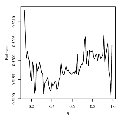
Figure 3 plots the estimated parameters of the skew-QBS-ACD model across q∈{0.01,…,0.99}q\in\{0.01,\ldots,0.99\}. Results suggest that this BASF-SE series displays asymmetric dynamics: the estimates of ϖ{\varpi} and σ{\sigma} tend to be increasing across qq, with a change of sign in the first case. On the other hand, the estimates of ρ\rho, α\alpha and λ\lambda appear to vary with the same pattern, but without an explicit trend.

Table 4: ML estimates (with SE in parentheses) and model selection measures for fit to the BASF-SE data.
EXP-ACD GG-ACD BS-ACD skew-QBS-ACD skew-QBS-ACD
(q=0.50q=0.50) (q=0.13q=0.13)
ϖ\varpi 0.0658 0.0724 −-0.2756 −-0.2362 -0.7723
(0.0180) (0.0183) (0.0975) (0.0822) (0.3034)
ρ\rho 0.6807 0.7204 0.5800 0.5948 0.5962
(0.1203) (0.0936) 0.1759 (0.1712) (0.1685)
σ\sigma 0.0937 0.1041 0.0403 0.0450 0.0119
(0.0206) (0.0211) (0.0107) (0.0118) (0.0031)
α\alpha 15.0013 1.1975 1.3060 1.3066
(6.5247) (0.0180) (0.0633) (0.0638)
ξ\xi 0.2467
(0.0547)
λ\lambda 0.5197 0.5213
(0.1578) (0.1586)
Log-lik. -2315.916 -2239.192 -2226.839 -2216.559 -2216.516
AIC 4637.832 4488.384 4461.659 4443.118 4443.033
BIC 4654.912 4516.851 4484.433 4471.585 4471.500
Q⁡(4)Q(4) 0.9451 0.9451 0.8152 0.8152 0.8141
Q⁡(16)Q(16) 0.3468 0.3468 0.2566 0.2566 0.2565
Refer to caption
(a) ϖ^\widehat{\varpi}
Refer to caption
(b) ρ^\widehat{\rho}
Refer to caption
(c) σ^\widehat{\sigma}
Refer to caption
(d) α^\widehat{\alpha}
Refer to caption
(e) λ^\widehat{\lambda}
Figure 3: Estimated parameters in the skew-QBS-ACD model across qq for the BASF-SE data.

Figure 4 shows the QQ plots with simulated envelope of the generalized Cox-Snell residuals for the models considered in Table 4. We see clearly that the skew-QBS-ACD models provide better fit than the EXP-ACD, GG-ACD and BS-ACD models.

Refer to caption
(a) EXP-ACD
Refer to caption
(b) GG-ACD
Refer to caption
(c) BS-ACD
Refer to caption
(d) skew-QBS-ACD(q=0.50q=0.50)
Refer to caption
(e) skew-QBS-ACD(q=0.13q=0.13)
Figure 4: QQ plot and its envelope for the generalized Cox-Snell residual in the indicated model with the BASF-SE data.

5.3 Forecasting performance

Figure 5 plots the in-sample and out-of-sample quantile forecasts from the adjusted skew-QBS-ACD and BS-ACD models. The construction of the plots is as follows. For each value of q∈{0.01,…,0.99}q\in\{0.01,\ldots,0.99\}, the skew-QBS-ACD model is estimated and the respective estimates are used to obtain the forecast of the quantile of interest. Since the BS-ACD model is independent of the value of qq, it is estimated only once and its forecasts are obtained from this single estimation. For in-sample forecasting, all data are used. In the case of out-of-sample forecasting, 2/3 of the data are used for estimation and the other 1/3 for forecasting.

From Figures 5(a,b), we observe that the forecasts of the skew-BS-ACD model are much closer to the actual values than those of the BS-ACD model. In fact, the forecasts of this latter model are quite far from the actual values. The superiority of the skew-QBS-ACD model may be due to different estimates obtained for the parameters; see, e.g., Figure 3. For different quantiles, we obtain different estimates, which makes the forecasts closer to the actual values. The results of the estimated mean square error (MSE) between the actual data and in-sample forecasted values of the adjusted skew-QBS-ACD and BS-ACD models are 0.041 and 1.277, respectively. Moreover, the MSE between the actual data and out-of-sample forecasted values of the adjusted skew-QBS-ACD and BS-ACD models are 0.029 and 1.199, respectively. Thus, the MSE values do confirm the results found in Figures 5(a,b).

Refer to caption
(a) In-sample
Refer to caption
(b) Out-of-sample
Figure 5: In-sample and out-of-sample quantile forecasts from the skew-QBS-ACD and BS-ACD models for the BASF-SE data.

6 Concluding remarks

In this paper, we have proposed a quantile autoregressive conditional duration model for dealing with high frequency financial duration data. The proposed model is based on a reparameterized version of the skewed Birnbaum-Saunders distribution, which has the distribution quantile as one of its parameters. Thus, the proposed conditional duration model is defined in terms of a conditional quantile duration, allowing different estimates for different quantiles of interest. A Monte Carlo simulation is carried out to evaluate the performance of the maximum likelihood estimators, study obtained by the ECM algorithm. We have applied the proposed and some other existing models to a real financial duration data set from the German DAX stock exchange. The results are seen to be quite favorable to the proposed model both in terms of model fitting and forecasting ability. The gain in considering the dynamics in terms of conditional quantile duration seems quite evident, especially in the forecasting superiority of the model. As part of future research, it will be of interest to use the theory of estimating functions for estimating the model parameters (Allen et al., 2013). Furthermore, quantile autoregressive conditional duration models can be used to estimate the intraday volatility of a stock (Tse and Yang, 2012). Work on these problems is currently in progress and we hope to report these findings in future papers.

Funding: Helton Saulo gratefully acknowledges financial support from FAP-DF.

References

  • Allen et al., (2013) Allen, D., Ng, K., and Peiris, S. (2013). Estimating and simulating Weibull models of risk or price durations: An application to ACD models. The North American Journal of Economics and Finance, 25:214–225.
  • Azzalini, (2019) Azzalini, A. (2019). The R package sn: The Skew-Normal and Related Distributions such as the Skew-tt (version 1.5-4). Università di Padova, Italia.
  • Azzalini and Capitanio, (2014) Azzalini, A. and Capitanio, A. (2014). The Skew-Normal and Related Families. Cambridge University Press, Cambridge, England.
  • Balakrishnan and Kundu, (2019) Balakrishnan, N. and Kundu, D. (2019). Birnbaum-saunders distribution: A review of models, analysis, and applications. Applied Stochastic Models in Business and Industry, 35:4–49.
  • Bauwens et al., (2003) Bauwens, L., Galli, F., and Giot, P. (2003). The moments of log-ACD models. CORE Discussion Paper, Available at SSRN: https://ssrn.com/abstract=375180 or http://dx.doi.org/10.2139/ssrn.375180.
  • Bhatti, (2010) Bhatti, C. (2010). The Birnbaum-Saunders autoregressive conditional duration model. Mathematics and Computers in Simulation, 80:2062–2078.
  • Bhogal and Variyam Thekke, (2019) Bhogal, S. K. and Variyam Thekke, R. (2019). Conditional duration models for high-frequency data: A review on recent developments. Journal of Economic Surveys, 33(1):252–273.
  • Birnbaum and Saunders, (1969) Birnbaum, Z. W. and Saunders, S. C. (1969). A new family of life distributions. Journal of Applied Probability, 6:319–327.
  • Davison, (2008) Davison, A. C. (2008). Statistical Models. Cambridge Series in Statistical and Probabilistic Mathematics, Cambridge University Press.
  • Engle and Russell, (1998) Engle, R. and Russell, J. (1998). Autoregressive conditional duration: A new method for irregularly spaced transaction data. Econometrica, 66:1127–1162.
  • Glaser, (1980) Glaser, R. E. (1980). Bathtub and related failure rate characterizations. Journal of the American Statistical Association, 75:667–672.
  • Koenker and Xiao, (2006) Koenker, R. and Xiao, Z. (2006). Quantile autoregression. Journal of the American Statistical Association, 101(475):980–990.
  • Pacurar, (2008) Pacurar, M. (2008). Autoregressive conditional durations models in finance: A survey of the theoretical and empirical literature. Journal of Economic Surveys, 22:711–751.
  • Sánchez et al., (2021) Sánchez, L., Leiva, V., Galea, M., and Saulo, H. (2021). Birnbaum-saunders quantile regression and its diagnostics with application to economic data. Applied Stochastic Models in Business and Industry, 37:53–73.
  • Saulo et al., (2019) Saulo, H., Leão, J., Leiva, V., and Aykroyd, R. G. (2019). Birnbaum-Saunders autoregressive conditional duration models applied to high-frequency financial data. Statistical Papers, 60:1605–1629.
  • Tse and Yang, (2012) Tse, Y.-k. and Yang, T. T. (2012). Estimation of high-frequency volatility: An autoregressive conditional duration approach. Journal of Business and Economic Statistics, 30.
  • Vilca and Leiva, (2006) Vilca, F. and Leiva, V. (2006). A new fatigue life model based on the family of skew-elliptical distributions. Communications in Statistics: Theory and Methods, 35:229–244.
  • Vilca et al., (2011) Vilca, F., Santana, L., Leiva, V., and Balakrishnan, N. (2011). Estimation of extreme percentiles in Birnbaum-Saunders distributions. Computational Statistics and Data Analysis, 55:1665–1678.

Appendix A Appendix

A.1 Some properties of the skew-QBS distribution

In this subsection, some results on the unimodality property, monotonicity of the hazard function, among others, of the skew-QBS distribution, are obtained.

Proposition 3 (Modes).

A mode of the skew-QBS(α,Ξq,λ)(\alpha,\Xi_{q},\lambda) is any point y0=y0​(α,Ξq,λ)y_{0}=y_{0}(\alpha,\Xi_{q},\lambda) that satisfies the following non-linear equation:

λ​[a′​(y,α,Ξq)]2​ϕ​[λ​a​(y,α,Ξq)]+Φ⁡[λ​a​(y,α,Ξq)]​{a′′​(y,α,Ξq)−a⁡(y,α,Ξq)​[a′​(y,α,Ξq)]2}=0.\lambda\big[a^{\prime}(y;\alpha,\Xi_{q})\big]^{2}\phi\big[\lambda a(y;\alpha,\Xi_{q})\big]+\Phi\big[\lambda a(y;\alpha,\Xi_{q})\big]\Big\{a^{\prime\prime}(y;\alpha,\Xi_{q})-a(y;\alpha,\Xi_{q})\Big[a^{\prime}(y;\alpha,\Xi_{q})\big]^{2}\Big\}=0.
Proof.

The proof is trivial and omitted. ∎

A.1.1 Unimodality property of the skew-QBS distribution

The following result provides sufficient conditions to guarantee unimodality of the skew-QBS distribution when the skewness parameter is positive.

Theorem 1 (Unimodality).

Let Y∼skew-QBS​(α,Ξq,λ)Y\sim\textrm{skew-QBS}(\alpha,\Xi_{q},\lambda) with λ>0\lambda>0. If fY′′′​(y,α,β,λ)≤0f^{\prime\prime\prime}_{Y}(y;\alpha,\beta,\lambda)\leq 0 for all y≥yBSy\geq y_{\rm BS}, where yBSy_{\rm BS} is the unique mode of the BS PDF satisfying the inequality

λ2​yBS3+Ξq​(2​α2+λ2)​yBS2+Ξq2​(3−λ2)​yBS−λ2​Ξq3>0,\displaystyle\lambda^{2}y_{\rm BS}^{3}+\Xi_{q}(2\alpha^{2}+\lambda^{2})y_{\rm BS}^{2}+\Xi_{q}^{2}(3-\lambda^{2})y_{\rm BS}-\lambda^{2}\Xi_{q}^{3}>0, (21)

then the skew-QBS PDF is unimodal.

Proof.

Let T∼BS​(α,Ξq)T\sim\textrm{BS}(\alpha,\Xi_{q}) be a random variable with BS PDF fT​(y,α,Ξq)f_{T}(y;\alpha,\Xi_{q}), y>0y>0. A simple computation shows that

fY′​(y,α,Ξq,λ)=\displaystyle f^{\prime}_{Y}(y;\alpha,\Xi_{q},\lambda)= 2​λ​a′​(y,α,Ξq)​ϕ​[λ​a​(y,α,Ξq)]​fT​(y,α,Ξq)\displaystyle 2\lambda a^{\prime}(y;\alpha,\Xi_{q})\phi\big[\lambda a(y;\alpha,\Xi_{q})\big]f_{T}(y;\alpha,\Xi_{q})
+2​Φ​[λ​a​(y,α,Ξq)]​fT′​(y,α,Ξq);\displaystyle+2\Phi\big[\lambda a(y;\alpha,\Xi_{q})\big]f^{\prime}_{T}(y;\alpha,\Xi_{q}); (22)
fY′′​(y,α,Ξq,λ)=\displaystyle f^{\prime\prime}_{Y}(y;\alpha,\Xi_{q},\lambda)= 2​λ​ϕ​[λ​a​(y,α,Ξq)]​[G⁡(y,α,Ξq,λ)​fT​(y,α,Ξq)+2​a′​(y,α,Ξq)​fT′​(y,α,Ξq)]\displaystyle 2\lambda\phi\big[\lambda a(y;\alpha,\Xi_{q})\big]\Big[G(y;\alpha,\Xi_{q},\lambda)f_{T}(y;\alpha,\Xi_{q})+2a^{\prime}(y;\alpha,\Xi_{q})f^{\prime}_{T}(y;\alpha,\Xi_{q})\Big]
+2​Φ​[λ​a​(y,α,Ξq)]​fT′′​(y,α,Ξq);\displaystyle+2\Phi\big[\lambda a(y;\alpha,\Xi_{q})\big]f^{\prime\prime}_{T}(y;\alpha,\Xi_{q}); (23)

where G⁡(y,α,Ξq,λ)G(y;\alpha,\Xi_{q},\lambda) is the function defined as

G⁡(y,α,Ξq,λ)=a′′​(y,α,Ξq)−λ2​a​(y,α,Ξq)​[a′​(y,α,Ξq)]2.\displaystyle G(y;\alpha,\Xi_{q},\lambda)=a^{\prime\prime}(y;\alpha,\Xi_{q})-\lambda^{2}a(y;\alpha,\Xi_{q})\big[a^{\prime}(y;\alpha,\Xi_{q})\big]^{2}.

By using the expression of the first derivative of a⁡(y,α,Ξq)a(y;\alpha,\Xi_{q}) given in (6), and the following second and third derivatives of a⁡(y,α,Ξq)a(y;\alpha,\Xi_{q}):

a′′​(y,α,Ξq)=−14​α​y2​[tΞq+3​Ξqy];a′′′​(y,α,Ξq)=38​α​y3​[yΞq+5​Ξqy];\displaystyle\begin{array}[]{lllll}\displaystyle a^{\prime\prime}(y;\alpha,\Xi_{q})=-\dfrac{1}{4\alpha y^{2}}\left[\sqrt{t\over\Xi_{q}}+3\sqrt{\Xi_{q}\over y}\right];&\displaystyle a^{\prime\prime\prime}(y;\alpha,\Xi_{q})=\dfrac{3}{8\alpha y^{3}}\left[\sqrt{y\over\Xi_{q}}+5\sqrt{\Xi_{q}\over y}\right];\end{array}

we can rewrite G⁡(y,α,Ξq,λ)G(y;\alpha,\Xi_{q},\lambda) as follows

G⁡(y,α,Ξq,λ)=−18​α3​Ξq3/2​y​[λ2​y3+Ξq​(2​α2+λ2)​y2+Ξq2​(3−λ2)​y−λ2​Ξq3].\displaystyle G(y;\alpha,\Xi_{q},\lambda)=-{1\over 8\alpha^{3}\Xi_{q}^{3/2}y}\,\Big[\lambda^{2}y^{3}+\Xi_{q}(2\alpha^{2}+\lambda^{2})y^{2}+\Xi_{q}^{2}(3-\lambda^{2})y-\lambda^{2}\Xi_{q}^{3}\Big]. (24)

In what follows we highlight the following remarks:

  • (a)

    For λ>0\lambda>0, a′​(y,α,Ξq)>0a^{\prime}(y;\alpha,\Xi_{q})>0 and fT′​(yBS,α,Ξq)=0f^{\prime}_{T}(y_{\rm BS};\alpha,\Xi_{q})=0, by (22), we have

    fY′​(yBS,α,Ξq,λ)=\displaystyle f^{\prime}_{Y}(y_{\rm BS};\alpha,\Xi_{q},\lambda)= 2​λ​a′​(yBS,α,Ξq)​ϕ​[λ​a​(yBS,α,Ξq)]​fT​(yBS,α,Ξq)>0.\displaystyle 2\lambda a^{\prime}(y_{\rm BS};\alpha,\Xi_{q})\phi\big[\lambda a(y_{\rm BS};\alpha,\Xi_{q})\big]f_{T}(y_{\rm BS};\alpha,\Xi_{q})>0.
  • (b)

    Since the unique mode of the BS PDF, yBSy_{\rm BS}, satisfies the inequality (21), from (24) it follows that G⁡(yBS,α,Ξq,λ)<0G(y_{\rm BS};\alpha,\Xi_{q},\lambda)<0. Hence, since fT′​(yBS,α,Ξq)=0f^{\prime}_{T}(y_{\rm BS};\alpha,\Xi_{q})=0 and fT′′​(yBS,α,Ξq)<0f^{\prime\prime}_{T}(y_{\rm BS};\alpha,\Xi_{q})<0, by (23), we get

    fY′′​(yBS,α,Ξq,λ)=\displaystyle f^{\prime\prime}_{Y}(y_{\rm BS};\alpha,\Xi_{q},\lambda)= 2​λ​ϕ​[λ​a​(yBS,α,Ξq)]​G​(yBS,α,Ξq,λ)​fT​(yBS,α,Ξq)\displaystyle 2\lambda\phi\big[\lambda a(y_{\rm BS};\alpha,\Xi_{q})\big]G(y_{\rm BS};\alpha,\Xi_{q},\lambda)f_{T}(y_{\rm BS};\alpha,\Xi_{q})
    +2​Φ​[λ​a​(yBS,α,Ξq)]​fT′′​(yBS,α,Ξq)<0.\displaystyle+2\Phi\big[\lambda a(y_{\rm BS};\alpha,\Xi_{q})\big]f^{\prime\prime}_{T}(y_{\rm BS};\alpha,\Xi_{q})<0.

Note that statements in Items (a) and (b), in addition to the hypothesis fY′′′​(y,α,Ξq,λ)≤0f^{\prime\prime\prime}_{Y}(y;\alpha,\Xi_{q},\lambda)\leq 0 for all y≥yBSy\geq y_{\rm BS}, guarantee that the function fY′​(y,α,Ξq,λ)f^{\prime}_{Y}(y;\alpha,\Xi_{q},\lambda) is decreasing and concave down. Hence, it follows that the function fY′​(y,α,Ξq,λ)f^{\prime}_{Y}(y;\alpha,\Xi_{q},\lambda) has a unique root, denoted by y0y_{0}, in the interval (yBS,+∞)(y_{\rm BS},+\infty). On the other hand, by unimodality of the BS distribution (Balakrishnan and Kundu, 2019), note that fT​(y,α,Ξq)f_{T}(y;\alpha,\Xi_{q}) is increasing on (0,yBS)(0,y_{\rm BS}), implying that the skew-QBS PDF fY​(y,α,Ξq,λ)f_{Y}(y;\alpha,\Xi_{q},\lambda) is also increasing on the interval (0,yBS)(0,y_{\rm BS}). Therefore, we obtain that y0y_{0} is the unique critical point for the function fY​(y,α,Ξq,λ)f_{Y}(y;\alpha,\Xi_{q},\lambda), y>0y>0. Finally, since limy→0+fY​(y,α,Ξq,λ)=0\lim_{y\to 0^{+}}f_{Y}(y;\alpha,\Xi_{q},\lambda)=0 and limy→+∞fY​(y,α,Ξq,λ)=0\lim_{y\to+\infty}f_{Y}(y;\alpha,\Xi_{q},\lambda)=0, we conclude that y0y_{0} is the unique mode of the skew-QBS distribution. ∎

A.1.2 Monotonicity of HR of the skew-QBS distribution

The survival and hazard functions, denoted by SF and HR of the skew-QBS distribution are given by SY​(y,α,Ξq,λ)=1−∫0yfY​(ξ,α,Ξq,λ)​𝑑ξS_{Y}(y;\alpha,\Xi_{q},\lambda)=1-\int_{0}^{y}f_{Y}(\xi;\alpha,\Xi_{q},\lambda)\,{\rm d}\xi, y>0y>0, and

HY​(y,α,Ξq,λ)\displaystyle H_{Y}(y;\alpha,\Xi_{q},\lambda) =fY​(y,α,Ξq,λ)SY​(y,α,Ξq,λ),y>0,\displaystyle={f_{Y}(y;\alpha,\Xi_{q},\lambda)\over S_{Y}(y;\alpha,\Xi_{q},\lambda)},\quad y>0,

respectively.

Proposition 4 (Monotonicity of HR).

Under the conditions of Theorem 1, the HR of the skew-QBS distribution has the following monotonic properties:

  • 1)

    It is increasing for all y<y0y<y_{0};

  • 2)

    It is decreasing for all y>y∗y>y_{*}, for some y∗≥y0y_{*}\geq y_{0};

where y0y_{0} is the mode of the skew-QBS density.

Proof.

By unimodality of the skew-QBS density (Theorem 1), the skew-QBS density fYf_{Y} increases on (0,y0)(0,y_{0}). Then, since the survival function SY​(y,α,Ξq,λ)S_{Y}(y;\alpha,\Xi_{q},\lambda), y>0y>0, is a decreasing function it follows that HY​(y,α,Ξq,λ)H_{Y}(y;\alpha,\Xi_{q},\lambda) is a product of two nonnegative increasing functions. Therefore, it is a increasing function for all y<y0y<y_{0}, and the proof of first item follows.

In order to prove the second item, by unimodality (Theorem 1), we have the existence of a point y∗≥y0y_{*}\geq y_{0} such that the skew-QBS density is a concave upward function on the interval J=(y∗,+∞)J=(y_{*},+\infty). That is, fY′′​(y,α,Ξq,λ)>0f_{Y}^{\prime\prime}(y;\alpha,\Xi_{q},\lambda)>0 for all Y∈JY\in J. Hence, fY′​(y,α,Ξq,λ)f_{Y}^{\prime}(y;\alpha,\Xi_{q},\lambda) is a decreasing function on JJ. Furthermore, by unimodality, the skew-QBS density fYf_{Y} decreases on this interval. Then the function GY​(y,α,Ξq,λ)G_{Y}(y;\alpha,\Xi_{q},\lambda), defined as

WY​(y,α,Ξq,λ)=−fY′​(y,α,Ξq,λ)fY​(y,α,Ξq,λ),\displaystyle W_{Y}(y;\alpha,\Xi_{q},\lambda)=-\,{f_{Y}^{\prime}(y;\alpha,\Xi_{q},\lambda)\over f_{Y}(y;\alpha,\Xi_{q},\lambda)},

decreases for all y∈Jy\in J, because WY​(y,α,Ξq,λ)W_{Y}(y;\alpha,\Xi_{q},\lambda), y∈Jy\in J, is a product of nonnegative decreasing functions. Hence, Glaser, 1980 guarantees that the HR HY​(y,α,Ξq,λ)H_{Y}(y;\alpha,\Xi_{q},\lambda) is a decreasing function for all y>y∗y>y_{*}. This completes the proof of Item 2). We thus complete the proof of proposition. ∎

A.1.3 Other properties of the skew-QBS distribution

Let Θq=2​erf−1​(q)\Theta_{q}=\sqrt{2}{\rm erf}^{-1}(q) be the 100​q100q-th quantile of the HN distribution, where erf−1{\rm erf}^{-1} is the inverse error function. The following proposition shows that the skew-QBS​(α,Ξq,λ)\textrm{skew-QBS}(\alpha,\Xi_{q},\lambda) distribution approaches the truncated BS​(α,Θq)\textrm{BS}(\alpha,\Theta_{q}) distribution with support [Θq,∞)[\Theta_{q},\infty), when the skewness parameter λ\lambda tends to infinity.

Proposition 5.

If Y∼skew-QBS​(α,Ξq,λ)Y\sim\textrm{skew-QBS}(\alpha,\Xi_{q},\lambda), the following properties hold:

  1. 1.

    limλ→∞fY​(y,α,Ξq,λ)=2​ϕ​[a⁡(y,α,Θq)]​a′​(y,α,Θq)​I[Θq,∞)​(y),\lim\limits_{\lambda\to\infty}f_{Y}(y;\alpha,\Xi_{q},\lambda)=2\phi\big[a(y;\alpha,\Theta_{q})\big]a^{\prime}(y;\alpha,\Theta_{q})\,I_{[\Theta_{q},\infty)}(y),\ for all y≠Θqy\neq\Theta_{q};

  2. 2.

    limλ→∞fY​(Θq,α,Ξq,λ)=(α​Θq​2​π)−1.\lim\limits_{\lambda\to\infty}f_{Y}(\Theta_{q};\alpha,\Xi_{q},\lambda)=\big(\alpha\Theta_{q}\sqrt{2\pi}\,\big)^{-1}.

Proof.

The proof is immediate upon observing that limλ→∞Ξq=Θq\lim_{\lambda\to\infty}\Xi_{q}=\Theta_{q}, limλ→∞a⁡(y,α,Ξq)=a⁡(y,α,Θq)\lim_{\lambda\to\infty}a(y;\alpha,\Xi_{q})=a(y;\alpha,\Theta_{q}) and limλ→∞a′​(y,α,Ξq)=a′​(y,α,Θq)\lim_{\lambda\to\infty}a^{\prime}(y;\alpha,\Xi_{q})=a^{\prime}(y;\alpha,\Theta_{q}). ∎

Proposition 6.

Let Y∼skew-QBS​(α,Ξq,λ)Y\sim\textrm{skew-QBS}(\alpha,\Xi_{q},\lambda). Then:

  1. 1.

    c​T∼skew-QBS​(α,c​Ξq,λ)cT\sim\textrm{skew-QBS}(\alpha,c\,\Xi_{q},\lambda), with c>0c>0;

  2. 2.

    T−1∼skew-QBS​(α,Ξq−1,−λ)T^{-1}\sim\textrm{skew-QBS}(\alpha,\Xi_{q}^{-1},-\lambda).

Proof.

The proof follows immediately through transformation of variables. ∎

Appendix B Appendix

The elements of the Hessian matrix are given by

∂2ℓ⁡(𝜽)∂γ​∂ϑ=\displaystyle{\partial^{2}{\ell}(\bm{\theta})\over\partial\gamma\partial\vartheta}= −∑t=1n1fY|Ξq2​(yt,α,Ξq,t,λ)∂fY|Ξq​(yt,α,Ξq,t,λ)∂γ∂fY|Ξq​(yt,α,Ξq,t,λ)∂ϑ\displaystyle-\sum_{t=1}^{n}\dfrac{1}{f^{2}_{Y|\Xi_{q}}(y_{t};\alpha,\Xi_{q,t},\lambda)}\,\dfrac{\partial f_{Y|\Xi_{q}}(y_{t};\alpha,\Xi_{q,t},\lambda)}{\partial\gamma}\,\dfrac{\partial f_{Y|\Xi_{q}}(y_{t};\alpha,\Xi_{q,t},\lambda)}{\partial\vartheta}
+∑t=1n1fY|Ξq​(yt,α,Ξq,t,λ)∂2fY|Ξq​(yt,α,Ξq,t,λ)∂γ​∂ϑ,\displaystyle+\sum_{t=1}^{n}\dfrac{1}{f_{Y|\Xi_{q}}(y_{t};\alpha,\Xi_{q,t},\lambda)}\,\dfrac{\partial^{2}f_{Y|\Xi_{q}}(y_{t};\alpha,\Xi_{q,t},\lambda)}{\partial\gamma\partial\vartheta},

for each γ,ϑ∈{α,ϖ,ρ1,…,ρr,σ1,…,σs,λ}\gamma,\vartheta\in\{\alpha,\varpi,\rho_{1},\ldots,\rho_{r},\sigma_{1},\ldots,\sigma_{s},\lambda\}, where

∂2fY|Ξq​(yt,α,Ξq,t,λ)∂γ​∂ϑ∗=2​Φ​[λ​a​(yt,α,Ξq,t,λ)]​∂2fT|Ξq​(yt,α,Ξq,t,λ)∂γ​∂ϑ∗\displaystyle{\partial^{2}f_{Y|\Xi_{q}}(y_{t};\alpha,\Xi_{q,t},\lambda)\over\partial\gamma\partial\vartheta^{*}}=2\Phi\big[\lambda a(y_{t};\alpha,\Xi_{q,t},\lambda)\big]\,{\partial^{2}f_{T|\Xi_{q}}(y_{t};\alpha,\Xi_{q,t},\lambda)\over\partial\gamma\partial\vartheta^{*}}
+2λϕ[λa(yt;α,Ξq,t,λ)]{∂a⁡(yt,α,Ξq,t,λ)∂γ∂fT|Ξq​(yt,α,Ξq,t,λ)∂ϑ∗+∂a⁡(yt,α,Ξq,t,λ)∂ϑ∗∂fT|Ξq​(yt,α,Ξq,t,λ)∂γ\displaystyle+2\lambda\phi\big[\lambda a(y_{t};\alpha,\Xi_{q,t},\lambda)\big]\bigg\{{\partial a(y_{t};\alpha,\Xi_{q,t},\lambda)\over\partial\gamma}\,{\partial f_{T|\Xi_{q}}(y_{t};\alpha,\Xi_{q,t},\lambda)\over\partial\vartheta^{*}}+{\partial a(y_{t};\alpha,\Xi_{q,t},\lambda)\over\partial\vartheta^{*}}\,{\partial f_{T|\Xi_{q}}(y_{t};\alpha,\Xi_{q,t},\lambda)\over\partial\gamma}
+[∂2a⁡(yt,α,Ξq,t,λ)∂γ​∂ϑ∗−λ2a(yt;α,Ξq,t,λ)∂a⁡(yt,α,Ξq,t,λ)∂γ∂a⁡(yt,α,Ξq,t,λ)∂ϑ∗]fT|Ξq(yt;α,Ξq,t,λ)}\displaystyle+\bigg[{\partial^{2}a(y_{t};\alpha,\Xi_{q,t},\lambda)\over\partial\gamma\partial\vartheta^{*}}-\lambda^{2}a(y_{t};\alpha,\Xi_{q,t},\lambda)\,{\partial a(y_{t};\alpha,\Xi_{q,t},\lambda)\over\partial\gamma}\,{\partial a(y_{t};\alpha,\Xi_{q,t},\lambda)\over\partial\vartheta^{*}}\bigg]f_{T|\Xi_{q}}(y_{t};\alpha,\Xi_{q,t},\lambda)\bigg\}

and

∂2fY|Ξq​(yt,α,Ξq,t,λ)∂γ​∂λ=∂2fY|Ξq​(yt,α,Ξq,t,λ)∂γ​∂ϑ∗+2​ϕ​[λ​a​(yt,α,Ξq,t,λ)]​fT|Ξq​(yt,α,Ξq,t,λ)​∂a⁡(yt,α,Ξq,t,λ)∂γ,\displaystyle{\partial^{2}f_{Y|\Xi_{q}}(y_{t};\alpha,\Xi_{q,t},\lambda)\over\partial\gamma\partial\lambda}={\partial^{2}f_{Y|\Xi_{q}}(y_{t};\alpha,\Xi_{q,t},\lambda)\over\partial\gamma\partial\vartheta^{*}}+2\phi\big[\lambda a(y_{t};\alpha,\Xi_{q,t},\lambda)\big]f_{T|\Xi_{q}}(y_{t};\alpha,\Xi_{q,t},\lambda)\,{\partial a(y_{t};\alpha,\Xi_{q,t},\lambda)\over\partial\gamma},

for each ϑ∗∈{α,ϖ,ρ1,…,ρr,σ1,…,σs}\vartheta^{*}\in\{\alpha,\varpi,\rho_{1},\ldots,\rho_{r},\sigma_{1},\ldots,\sigma_{s}\}, with

∂2fT|Ξq​(yt,α,Ξq,t,λ)∂γ​∂ϑ=−a⁡(yt,α,Ξq,t,λ)​∂a⁡(yt,α,Ξq,t,λ)∂ϑ​∂fT|Ξq​(yt,α,Ξq,t,λ)∂ϑ\displaystyle{\partial^{2}f_{T|\Xi_{q}}(y_{t};\alpha,\Xi_{q,t},\lambda)\over\partial\gamma\partial\vartheta}=-a(y_{t};\alpha,\Xi_{q,t},\lambda)\,{\partial a(y_{t};\alpha,\Xi_{q,t},\lambda)\over\partial\vartheta}\,{\partial f_{T|\Xi_{q}}(y_{t};\alpha,\Xi_{q,t},\lambda)\over\partial\vartheta}
+ϕ[a(yt;α,Ξq,t,λ)]{∂2a′​(yt,α,Ξq,t,λ)∂γ​∂ϑ−a(yt;α,Ξq,t,λ)a′(yt;α,Ξq,t,λ)∂2a⁡(yt,α,Ξq,t,λ)∂γ​∂ϑ\displaystyle+\phi\big[a(y_{t};\alpha,\Xi_{q,t},\lambda)\big]\bigg\{{\partial^{2}a^{\prime}(y_{t};\alpha,\Xi_{q,t},\lambda)\over\partial\gamma\partial\vartheta}-a(y_{t};\alpha,\Xi_{q,t},\lambda)a^{\prime}(y_{t};\alpha,\Xi_{q,t},\lambda)\,{\partial^{2}a(y_{t};\alpha,\Xi_{q,t},\lambda)\over\partial\gamma\partial\vartheta}
−[∂a⁡(yt,α,Ξq,t,λ)∂ϑa′(yt;α,Ξq,t,λ)+a(yt;α,Ξq,t,λ)∂a′​(yt,α,Ξq,t,λ)∂ϑ]},\displaystyle-\bigg[{\partial a(y_{t};\alpha,\Xi_{q,t},\lambda)\over\partial\vartheta}\,a^{\prime}(y_{t};\alpha,\Xi_{q,t},\lambda)+a(y_{t};\alpha,\Xi_{q,t},\lambda)\,{\partial a^{\prime}(y_{t};\alpha,\Xi_{q,t},\lambda)\over\partial\vartheta}\bigg]\bigg\},

for each γ,ϑ∈{α,ϖ,ρ1,…,ρr,σ1,…,σs,λ}\gamma,\vartheta\in\{\alpha,\varpi,\rho_{1},\ldots,\rho_{r},\sigma_{1},\ldots,\sigma_{s},\lambda\}. A simple computation shows that the above second order partial derivatives of functions a⁡(yt,α,Ξq,t,λ)a(y_{t};\alpha,\Xi_{q,t},\lambda) and a′​(yt,α,Ξq,t,λ)a^{\prime}(y_{t};\alpha,\Xi_{q,t},\lambda) are expressed as

∂2a⁡(yt,α,Ξq,t,λ)∂α2\displaystyle\textstyle{\partial^{2}a(y_{t};\alpha,\Xi_{q,t},\lambda)\over\partial\alpha^{2}} =a⁡(yt,α,Ξq,t,λ)α2−1α​∂a⁡(yt,α,Ξq,t,λ)∂α+2​a′​(yt,α,Ξq,t,λ)​ηα;λ​∂2ηα;λ∂α2\displaystyle=\textstyle{a(y_{t};\alpha,\Xi_{q,t},\lambda)\over\alpha^{2}}-{1\over\alpha}\,{\partial a(y_{t};\alpha,\Xi_{q,t},\lambda)\over\partial\alpha}+2a^{\prime}(y_{t};\alpha,\Xi_{q,t},\lambda)\eta_{\alpha;\lambda}\,{\partial^{2}\eta_{\alpha;\lambda}\over\partial\alpha^{2}}
+2​[∂a′​(yt,α,Ξq,t,λ)∂α​ηα;λ+a′​(yt,α,Ξq,t,λ)​∂ηα;λ∂α]​∂ηα;λ∂α,\displaystyle\quad+\textstyle 2\big[{\partial a^{\prime}(y_{t};\alpha,\Xi_{q,t},\lambda)\over\partial\alpha}\,\eta_{\alpha;\lambda}+a^{\prime}(y_{t};\alpha,\Xi_{q,t},\lambda)\,{\partial\eta_{\alpha;\lambda}\over\partial\alpha}\big]{\partial\eta_{\alpha;\lambda}\over\partial\alpha},
∂2a⁡(yt,α,Ξq,t,λ)∂α​∂γ∗\displaystyle\textstyle{\partial^{2}a(y_{t};\alpha,\Xi_{q,t},\lambda)\over\partial\alpha\partial\gamma^{*}} =−1α​∂a⁡(yt,α,Ξq,t,λ)∂γ∗+2​∂a′​(yt,α,Ξq,t,λ)∂γ∗​∂ηα;λ∂α​ηα;λ,γ∗∈{ϖ,ρk,σl},\displaystyle=\textstyle-{1\over\alpha}\,{\partial a(y_{t};\alpha,\Xi_{q,t},\lambda)\over\partial\gamma^{*}}+2\,{\partial a^{\prime}(y_{t};\alpha,\Xi_{q,t},\lambda)\over\partial\gamma^{*}}\,{\partial\eta_{\alpha;\lambda}\over\partial\alpha}\,\eta_{\alpha;\lambda},\quad\gamma^{*}\in\{\varpi,\rho_{k},\sigma_{l}\},
∂2a⁡(yt,α,Ξq,t,λ)∂α​∂λ\displaystyle\textstyle{\partial^{2}a(y_{t};\alpha,\Xi_{q,t},\lambda)\over\partial\alpha\partial\lambda} =−1α​∂a⁡(yt,α,Ξq,t,λ)∂λ+2​a′​(yt,α,Ξq,t,λ)​ηα;λ​∂2ηα;λ∂α​∂λ\displaystyle=\textstyle-{1\over\alpha}\,{\partial a(y_{t};\alpha,\Xi_{q,t},\lambda)\over\partial\lambda}+2a^{\prime}(y_{t};\alpha,\Xi_{q,t},\lambda)\eta_{\alpha;\lambda}\,{\partial^{2}\eta_{\alpha;\lambda}\over\partial\alpha\partial\lambda}
+2​[∂a′​(yt,α,Ξq,t,λ)∂λ​ηα;λ+a′​(yt,α,Ξq,t,λ)​∂ηα;λ∂λ]​∂ηα;λ∂α,\displaystyle\quad+\textstyle 2\big[{\partial a^{\prime}(y_{t};\alpha,\Xi_{q,t},\lambda)\over\partial\lambda}\,\eta_{\alpha;\lambda}+a^{\prime}(y_{t};\alpha,\Xi_{q,t},\lambda)\,{\partial\eta_{\alpha;\lambda}\over\partial\lambda}\big]{\partial\eta_{\alpha;\lambda}\over\partial\alpha},
∂2a⁡(yt,α,Ξq,t,λ)∂γ∗​∂ϑ∗\displaystyle\textstyle{\partial^{2}a(y_{t};\alpha,\Xi_{q,t},\lambda)\over\partial\gamma^{*}\partial\vartheta^{*}} =[2Ξq,t−∂a′​(yt,α,Ξq,t,λ)∂ϑ∗]​1Ξq,t2​∂Ξq,t∂γ∗−a′​(yt,α,Ξq,t,λ)Ξq,t​∂2Ξq,t∂γ∗​∂ϑ∗,γ∗,ϑ∗∈{ϖ,ρk,σl},\displaystyle=\textstyle\big[{2\over\Xi_{q,t}}-{\partial a^{\prime}(y_{t};\alpha,\Xi_{q,t},\lambda)\over\partial\vartheta^{*}}\big]{1\over\Xi^{2}_{q,t}}\,{\partial\Xi_{q,t}\over\partial\gamma^{*}}-{a^{\prime}(y_{t};\alpha,\Xi_{q,t},\lambda)\over\Xi_{q,t}}\,{\partial^{2}\Xi_{q,t}\over\partial\gamma^{*}\partial\vartheta^{*}},\quad\gamma^{*},\vartheta^{*}\in\{\varpi,\rho_{k},\sigma_{l}\},
∂2a⁡(yt,α,Ξq,t,λ)∂γ∗​∂λ\displaystyle\textstyle{\partial^{2}a(y_{t};\alpha,\Xi_{q,t},\lambda)\over\partial\gamma^{*}\partial\lambda} =−1Ξq,t2​∂a′​(yt,α,Ξq,t,λ)∂λ​∂Ξq,t∂γ∗,\displaystyle=\textstyle-{1\over\Xi_{q,t}^{2}}\,{\partial a^{\prime}(y_{t};\alpha,\Xi_{q,t},\lambda)\over\partial\lambda}\,{\partial\Xi_{q,t}\over\partial\gamma^{*}},
∂2a⁡(yt,α,Ξq,t,λ)∂λ2\displaystyle\textstyle{\partial^{2}a(y_{t};\alpha,\Xi_{q,t},\lambda)\over\partial\lambda^{2}} =+2​a′​(yt,α,Ξq,t,λ)​ηα;λ​∂2ηα;λ∂λ2\displaystyle=\textstyle+2a^{\prime}(y_{t};\alpha,\Xi_{q,t},\lambda)\eta_{\alpha;\lambda}\,{\partial^{2}\eta_{\alpha;\lambda}\over\partial\lambda^{2}}
+2​[∂a′​(yt,α,Ξq,t,λ)∂λ​ηα;λ+a′​(yt,α,Ξq,t,λ)​∂ηα;λ∂λ]​∂ηα;λ∂λ,\displaystyle\quad+\textstyle 2\big[{\partial a^{\prime}(y_{t};\alpha,\Xi_{q,t},\lambda)\over\partial\lambda}\,\eta_{\alpha;\lambda}+a^{\prime}(y_{t};\alpha,\Xi_{q,t},\lambda)\,{\partial\eta_{\alpha;\lambda}\over\partial\lambda}\big]{\partial\eta_{\alpha;\lambda}\over\partial\lambda},

where ηα;λ\eta_{\alpha;\lambda} is as in (12), k=1,…,rk=1,\ldots,r and l=1,…,sl=1,\ldots,s, and

∂2a′​(yt,α,Ξq,t,λ)∂α2\displaystyle\textstyle{\partial^{2}a^{\prime}(y_{t};\alpha,\Xi_{q,t},\lambda)\over\partial\alpha^{2}} =a′​(yt,α,Ξq,t,λ)α2−1α​∂a′​(yt,α,Ξq,t,λ)∂α+2​a′′​(yt,α,Ξq,t,λ)​ηα;λ​∂2ηα;λ∂α2\displaystyle=\textstyle{a^{\prime}(y_{t};\alpha,\Xi_{q,t},\lambda)\over\alpha^{2}}-{1\over\alpha}\,{\partial a^{\prime}(y_{t};\alpha,\Xi_{q,t},\lambda)\over\partial\alpha}+2a^{\prime\prime}(y_{t};\alpha,\Xi_{q,t},\lambda)\eta_{\alpha;\lambda}\,{\partial^{2}\eta_{\alpha;\lambda}\over\partial\alpha^{2}}
+2​[∂a′′​(yt,α,Ξq,t,λ)∂α​ηα;λ+a′′​(yt,α,Ξq,t,λ)​∂ηα;λ∂α]​∂ηα;λ∂α,\displaystyle\quad+\textstyle 2\big[{\partial a^{\prime\prime}(y_{t};\alpha,\Xi_{q,t},\lambda)\over\partial\alpha}\,\eta_{\alpha;\lambda}+a^{\prime\prime}(y_{t};\alpha,\Xi_{q,t},\lambda)\,{\partial\eta_{\alpha;\lambda}\over\partial\alpha}\big]{\partial\eta_{\alpha;\lambda}\over\partial\alpha},
∂2a′​(yt,α,Ξq,t,λ)∂α​∂γ∗\displaystyle\textstyle{\partial^{2}a^{\prime}(y_{t};\alpha,\Xi_{q,t},\lambda)\over\partial\alpha\partial\gamma^{*}} =−1α​∂a′​(yt,α,Ξq,t,λ)∂γ∗+2​∂a′′​(yt,α,Ξq,t,λ)∂γ∗​∂ηα;λ∂α​ηα;λ,γ∗∈{ϖ,ρk,σl},\displaystyle=\textstyle-{1\over\alpha}\,{\partial a^{\prime}(y_{t};\alpha,\Xi_{q,t},\lambda)\over\partial\gamma^{*}}+2\,{\partial a^{\prime\prime}(y_{t};\alpha,\Xi_{q,t},\lambda)\over\partial\gamma^{*}}\,{\partial\eta_{\alpha;\lambda}\over\partial\alpha}\,\eta_{\alpha;\lambda},\quad\gamma^{*}\in\{\varpi,\rho_{k},\sigma_{l}\},
∂2a′​(yt,α,Ξq,t,λ)∂α​∂λ\displaystyle\textstyle\textstyle{\partial^{2}a^{\prime}(y_{t};\alpha,\Xi_{q,t},\lambda)\over\partial\alpha\partial\lambda} =−1α​∂a′​(yt,α,Ξq,t,λ)∂λ+2​a′′​(yt,α,Ξq,t,λ)​ηα;λ​∂2ηα;λ∂α​∂λ\displaystyle=\textstyle-{1\over\alpha}\,{\partial a^{\prime}(y_{t};\alpha,\Xi_{q,t},\lambda)\over\partial\lambda}+2a^{\prime\prime}(y_{t};\alpha,\Xi_{q,t},\lambda)\eta_{\alpha;\lambda}\,{\partial^{2}\eta_{\alpha;\lambda}\over\partial\alpha\partial\lambda}
+2​[∂a′′​(yt,α,Ξq,t,λ)∂λ​ηα;λ+a′′​(yt,α,Ξq,t,λ)​∂ηα;λ∂λ]​∂ηα;λ∂α,\displaystyle\quad+\textstyle 2\big[{\partial a^{\prime\prime}(y_{t};\alpha,\Xi_{q,t},\lambda)\over\partial\lambda}\,\eta_{\alpha;\lambda}+a^{\prime\prime}(y_{t};\alpha,\Xi_{q,t},\lambda)\,{\partial\eta_{\alpha;\lambda}\over\partial\lambda}\big]{\partial\eta_{\alpha;\lambda}\over\partial\alpha},
∂2a′​(yt,α,Ξq,t,λ)∂γ∗​∂ϑ∗\displaystyle\textstyle{\partial^{2}a^{\prime}(y_{t};\alpha,\Xi_{q,t},\lambda)\over\partial\gamma^{*}\partial\vartheta^{*}} =[2Ξq,t−∂a′′​(yt,α,Ξq,t,λ)∂ϑ∗]​1Ξq,t2​∂Ξq,t∂γ∗−a′′​(yt,α,Ξq,t,λ)Ξq,t​∂2Ξq,t∂γ∗​∂ϑ∗,γ∗,ϑ∗∈{ϖ,ρk,σl},\displaystyle=\textstyle\big[{2\over\Xi_{q,t}}-{\partial a^{\prime\prime}(y_{t};\alpha,\Xi_{q,t},\lambda)\over\partial\vartheta^{*}}\big]{1\over\Xi^{2}_{q,t}}\,{\partial\Xi_{q,t}\over\partial\gamma^{*}}-{a^{\prime\prime}(y_{t};\alpha,\Xi_{q,t},\lambda)\over\Xi_{q,t}}\,{\partial^{2}\Xi_{q,t}\over\partial\gamma^{*}\partial\vartheta^{*}},\quad\gamma^{*},\vartheta^{*}\in\{\varpi,\rho_{k},\sigma_{l}\},
∂2a′​(yt,α,Ξq,t,λ)∂γ∗​∂λ\displaystyle\textstyle{\partial^{2}a^{\prime}(y_{t};\alpha,\Xi_{q,t},\lambda)\over\partial\gamma^{*}\partial\lambda} =−1Ξq,t2​∂a′′​(yt,α,Ξq,t,λ)∂λ​∂Ξq,t∂γ∗,\displaystyle=\textstyle-{1\over\Xi_{q,t}^{2}}\,{\partial a^{\prime\prime}(y_{t};\alpha,\Xi_{q,t},\lambda)\over\partial\lambda}\,{\partial\Xi_{q,t}\over\partial\gamma^{*}},
∂2a′​(yt,α,Ξq,t,λ)∂λ2\displaystyle\textstyle{\partial^{2}a^{\prime}(y_{t};\alpha,\Xi_{q,t},\lambda)\over\partial\lambda^{2}} =+2​a′′​(yt,α,Ξq,t,λ)​ηα;λ​∂2ηα;λ∂λ2\displaystyle=\textstyle+2a^{\prime\prime}(y_{t};\alpha,\Xi_{q,t},\lambda)\eta_{\alpha;\lambda}\,{\partial^{2}\eta_{\alpha;\lambda}\over\partial\lambda^{2}}
+2​[∂a′′​(yt,α,Ξq,t,λ)∂λ​ηα;λ+a′′​(yt,α,Ξq,t,λ)​∂ηα;λ∂λ]​∂ηα;λ∂λ,\displaystyle\quad+\textstyle 2\big[{\partial a^{\prime\prime}(y_{t};\alpha,\Xi_{q,t},\lambda)\over\partial\lambda}\,\eta_{\alpha;\lambda}+a^{\prime\prime}(y_{t};\alpha,\Xi_{q,t},\lambda)\,{\partial\eta_{\alpha;\lambda}\over\partial\lambda}\big]{\partial\eta_{\alpha;\lambda}\over\partial\lambda},

for each k=1,…,rk=1,\ldots,r and l=1,…,sl=1,\ldots,s, with

∂a′′​(yt,α,Ξq,t,λ)∂α\displaystyle\textstyle{\partial a^{\prime\prime}(y_{t};\alpha,\Xi_{q,t},\lambda)\over\partial\alpha} =−a′′​(yt,α,Ξq,t,λ)2​α​yt+2​a′′′​(yt,α,Ξq,t,λ)​ηα;λ​∂ηα;λ∂α,\displaystyle=\textstyle-{a^{\prime\prime}(y_{t};\alpha,\Xi_{q,t},\lambda)\over 2\alpha y_{t}}+2a^{\prime\prime\prime}(y_{t};\alpha,\Xi_{q,t},\lambda)\eta_{\alpha;\lambda}\,{\partial\eta_{\alpha;\lambda}\over\partial\alpha},
∂a′′​(yt,α,Ξq,t,λ)∂γ∗\displaystyle\textstyle{\partial a^{\prime\prime}(y_{t};\alpha,\Xi_{q,t},\lambda)\over\partial\gamma^{*}} =−a′′′​(yt,α,Ξq,t,λ)​1Ξq,t2​∂Ξq,t∂γ∗,γ∗∈{ϖ,ρ1,…,ρr,σ1,…,σs},\displaystyle=\textstyle-a^{\prime\prime\prime}(y_{t};\alpha,\Xi_{q,t},\lambda)\,{1\over\Xi_{q,t}^{2}}\,{\partial\Xi_{q,t}\over\partial\gamma^{*}},\quad\gamma^{*}\in\{\varpi,\rho_{1},\ldots,\rho_{r},\sigma_{1},\ldots,\sigma_{s}\},
∂a′′​(yt,α,Ξq,t,λ)∂λ\displaystyle\textstyle{\partial a^{\prime\prime}(y_{t};\alpha,\Xi_{q,t},\lambda)\over\partial\lambda} =2​a′′′​(yt,α,Ξq,t,λ)​ηα;λ​∂ηα;λ∂λ,\displaystyle=\textstyle 2a^{\prime\prime\prime}(y_{t};\alpha,\Xi_{q,t},\lambda)\eta_{\alpha;\lambda}\,{\partial\eta_{\alpha;\lambda}\over\partial\lambda},

and

a′′′​(yt,α,Ξq,t,λ)=38​α​yt3​[yt​ηα;λ24​Ξq,t+5​4​Ξq,tyt​ηα;λ2].\displaystyle a^{\prime\prime\prime}(y_{t};\alpha,\Xi_{q,t},\lambda)={3\over 8\alpha y^{3}_{t}}\left[\sqrt{\frac{y_{t}\eta_{\alpha;\lambda}^{2}}{4\Xi_{q,t}}}+5\sqrt{\frac{4\Xi_{q,t}}{y_{t}\eta_{\alpha;\lambda}^{2}}}\right].