Bosonic Dark Matter in Neutron Stars and its Effect on Gravitational Wave Signal

Despite enormous efforts during the past three decades, the nature of dark matter (DM) still remains unknown. Currently there are several motivated particle candidates for DM such as Weakly Interacting Massive Particles (WIMPs), axions, sterile neutrinos, etc Bertone and Tait 2018; Bertone and Hooper 2018. Research into the detectability of these particles has revealed a vast number of promising experimental facilities ranging from high-precision table-top experiments to incorporating astronomical surveys and Gravitational-Wave (GW) observations.

The terrestrial experiments have been operating during the years in order to detect DM particles, including the recoil experiments that aim to measure the direct evidence of the interaction between the new particle and nuclear or atomic targets Mayet et al. 2016; Billard et al. 2021; Roberts and Flambaum 2019; Catena et al. 2020. Due to the null results achieved in the direct DM searches with masses larger than a few GeV in the past years, recently an increase of detection efforts have been conducted in the sub-GeV region, which has a mass between 1 keV and the mass of proton Kouvaris and Pradler 2017; Essig et al. 2019; Aprile et al. 2019; Essig et al. 2017. The sub-GeV mass range is relatively unexplored because of the experimental challenges of detecting such light DM particles with traditional techniques. Recently, the XENON1T collaboration observed a $3.5\sigma$ excess of events from recoil electrons Aprile et al. 2020 which might be the evidence for the existence of DM particles with masses around $90\ \text{keV}$ Shakeri et al. 2020.

Other existing DM search strategies are the decay of known particle into the DM particles, e.g, the anomalous decay of B-meson reported by the LHCb collaboration Cerdeño et al. 2019, and indirect searches which are looking for self-annihilation signal generated by DM particles at the Galactic center Argüelles et al. 2019; Slatyer 2016; Brdar et al. 2018.

On the other hand, compact astrophysical objects such as neutron stars (NSs) can capture a sizable amount of DM which provide a unique astrophysical laboratory to indirectly probe the nature of DM. The presence of DM can substantially alter the star’s structure and its thermodynamic properties leading to observable signals from astrophysical measurements Panotopoulos and Lopes 2017; Nelson et al. 2019; Ellis et al. 2018a; Ivanytskyi et al. 2020; Rezaei 2017; de Lavallaz and Fairbairn 2010; Gresham and Zurek 2019. An accretion of self-annihilating DM into a NS can be detected via increasing the luminosity and the effective temperature Kouvaris 2008; Bhat and Paul 2020; Fuller and Ott 2015; Acevedo et al. 2021a or by modifying the cooling curves of the star of a certain mass Sedrakian 2019; Sedrakian 2016. However, DM particles with negligible annihilation rate will settle within the NSs. This scenario is realized as Asymmetric Dark Matter (ADM) in which a particle-antiparticle asymmetry in the dark sector exists similar to one of the baryon asymmetry in the Universe Kaplan et al. 2009; Shelton and Zurek 2010; Petraki and Volkas 2013; Kouvaris and Nielsen 2015a. Non-annihilating ADM whether fermionic or bosonic nature might form stable compact object named dark stars Narain et al. 2006; Kouvaris and Nielsen 2015a; Eby et al. 2016. Accumulation of ADM in NS could continue until a black hole (BH) formation which can tightly constraint ADM models by the presence of old NSs McDermott et al. 2012; Bertone and Fairbairn 2008; Kouvaris and Tinyakov 2011a; Kouvaris and Tinyakov 2011b; Acevedo et al. 2021b; Khlopov et al. 1985.

It has been shown that an accretion of massive ADM particles can significantly reduce the maximum mass of the host NS making the two solar mass limit unattainable Xiang et al. 2014; Leung et al. 2011; Li et al. 2012a; Deliyergiyev et al. 2019. Thus, observational fact of an existence of two heavy pulsars, i.e, PSR J0348+0432 with mass $2.01\pm 0.04M_{\odot}$ Antoniadis et al. 2013 and PSR J0740+6620 of $2.14^{+0.10}_{-0.09}M_{\odot}$ Cromartie et al. 2019, enables us to constrain the properties of massive DM particles and their fraction inside the compact stars. On the other hand, light DM particles lead to formation of an extended halo around the NS and could increase its total gravitational mass Ivanytskyi et al. 2020; Nelson et al. 2019.

Based on the NS observations, it has been argued that the presence of light bosonic ADM without self-interaction has been excluded in the mass range $2\ \text{keV}$ - $16\ \text{GeV}$ due to the BH formation Kouvaris and Tinyakov 2011b. Furthermore, a similar result has been reported about tight constraints on the noninteracting scalar ADM with masses between 5 MeV and 13 GeV McDermott et al. 2012. The observed discrepancy in the low-mass region reported in Ref. Kouvaris and Tinyakov 2011b and Ref. McDermott et al. 2012 is because of an inclusion of an effect of neutron degeneracy on the capture rate in the latter case. However, it was shown that taking into account a repulsive self-interaction among DM particles prevents instability issues related to the BH formation Bell et al. 2013; Kouvaris 2013; Nelson et al. 2019; Mielke and Schunck 2000; Ho et al. 1999. In addition, self-interacting DM can resolve a series of issues in the collisionless cold DM (CCDM) scenario for the small-scale cosmological observations Rocha et al. 2013; Vogelsberger et al. 2012; Zavala et al. 2013; Argüelles et al. 2016. The self-interaction cross section per unit DM mass in range $0.1\ \text{cm}^{2}/\text{gr}\lesssim\sigma/m\lesssim 1\ \text{cm}^{2}/\text{gr}$ is sufficient to explain various inconsistencies between numerical simulations and observational results in CCDM paradigm Giudice et al. 2016; Eby et al. 2016; Amaro-Seoane et al. 2010; Peter et al. 2013; Kaplinghat et al. 2016. Moreover, it has been shown that a self-interacting complex scalar field can form a Bose-Einstein condensate (BEC) which yields an attractive solution for the DM Galactic halo and other astronomical DM issues Arbey et al. 2003; Suárez et al. 2014; Suárez and Chavanis 2015; Boehmer and Harko 2007; Li et al. 2014; Chavanis 2017; Sikivie and Yang 2009; Harko 2011; Chavanis and Harko 2012; Suárez and Chavanis 2017.

The stability of a self-gravitating system of fermionic DM particles without self-interaction is provided by the Fermi pressure. For bosonic DM the only source of pressure against the gravitational contraction comes from the uncertainty principle leading to formation of Boson Stars (BSs), for a comprehensive review on BSs see Schunck and Mielke 2003; Liebling and Palenzuela 2017; Visinelli 2021. Historically, the idea of BS was proposed by Kaup 1968, Ruffini and Bonazzola 1969, they showed that BSs consisting of noninteracting particles have much lower maximum mass compared to their fermionic counterparts. However, introducing the repulsive interaction between bosons, e.g, proposed by Colpi et al. 1986, drastically changes the physical properties of BSs. Depending on the mass and strength of the self-interaction between DM particles, BSs of stellar mass could have observable signatures at GW detectors Pacilio et al. 2020; Giudice et al. 2016. Therefore, either self-interacting bosonic ADM as the complex scalar field or ultra light axions without self-interaction could form a dark BS of the stellar mass Gleiser 1988; Kusmartsev et al. 1991; Kolb and Tkachev 1993; Schunck and Mielke 1998; Mielke and Schunck 2000; Chavanis and Harko 2012; Maselli et al. 2017; Eby et al. 2016; Chavanis and Delfini 2011; Chavanis 2011; Visinelli et al. 2018; Chavanis 2018; Kouvaris et al. 2020. As other possibilities, the dark BS can be formed in terms of a Bose-Einstein gravitational condensation described by Gross-Pitaevskii-Poisson equation Chavanis and Harko 2012; Li et al. 2012b, or it can be made of bosons with a repulsive self-interaction described within the mean-field approximation and general relativity Agnihotri et al. 2009. Both above mentioned dark BS models were utilized as a DM component within NSs Nelson et al. 2019; Li et al. 2012c; Ellis et al. 2018a.

Generally, three different scenarios can be realized for a DM admixed NS Mukhopadhyay et al. 2017; Li et al. 2012c; Goldman et al. 2013; Tolos and Schaffner-Bielich 2015 :
(i) DM is condensed in a NS core. In this case, radius of DM component ($R_{D}$) is smaller than radius of baryonic matter (BM) component ($R_{B}$), i.e, $R_{B}>R_{D}$;
(ii) DM distributed in entire NS with $R_{B}=R_{D}$;
(iii) DM creates an extended halo around a NS with $R_{D}>R_{B}$.
The above mentioned configurations are valid for only gravitational interaction between BM and DM, allowing a mixture of both fluids at the core and the possible appearance of one of them at the outer shell of the combined object Nelson et al. 2019; Ellis et al. 2018a; Xiang et al. 2014; Goldman et al. 2013; Tolos and Schaffner-Bielich 2015; Sandin and Ciarcelluti 2009; Ciarcelluti and Sandin 2011; Mukhopadhyay et al. 2017; Deliyergiyev et al. 2019; Mukhopadhyay and Schaffner-Bielich 2016; Ivanytskyi et al. 2020.

In the case of sufficiently strong nongravitational interaction between both components their mixing is prevented leading to two more scenarios. One of them corresponds to a star with a pure baryonic core surrounded by a DM halo, while the other one describes a star with a pure DM core and a baryonic shell Gresham and Zurek 2019; Li et al. 2012c; Zhang et al. 2020; Zhang and Lin 2020. Meanwhile, in the presence of the nongravitational interactions between BM and DM, the whole system can be described by a single equation of state (EoS) obtained from the relativistic mean-field model Panotopoulos and Lopes 2017; Gresham and Zurek 2019; Das et al. 2019a; Das et al. 2020a; Sen and Guha 2021; Das et al. 2021.

The recent detections of GWs from the binary NS mergers opened a new window for probing DM particles Abbott et al. 2017; Abbott et al. 2020a. The impact of ADM particles on the internal structure of NSs can be considered through GW signals especially during the post-merger stage Ellis et al. 2018b; Bezares et al. 2019; Bezares and Palenzuela 2018; Horowitz and Reddy 2019; Bauswein et al. 2020. The GW signal is also sensitive to the deformation effects of binary NSs during the inspiral phase. This information encodes in the tidal deformability parameter which gives valuable clues into the EoS of NSs Hinderer 2008; Hinderer et al. 2010; Postnikov et al. 2010; Zhao and Lattimer 2018; Han and Steiner 2019. The upper bound on tidal deformability $\Lambda\leq 800$ for $M=1.4M_{\odot}$ was obtained by the GW observation at the $90\%$ confidence level for GW170817 created by coalescence of the binary NSs Abbott et al. 2017. An improved estimate of $\Lambda_{1.4}=190^{+390}_{-120}$ has been reported in Abbott et al. 2018. It is worth mentioning that most of BM EoSs obtained from many-body theories, taking into account the realistic nucleon-nucleon interactions Nelson et al. 2019; Gandolfi et al. 2012; Hebeler et al. 2015; Tews et al. 2018; Hebeler et al. 2010; Goudarzi et al. 2018; Fattoyev et al. 2018; Dengler et al. 2021, produce the tidal deformability in the range of 100-500. The presence of DM in NSs will alter the tidal deformability which can be utilized to probe the parameter space of DM model and the amount of DM within NSs to be consistent with observational constraints Nelson et al. 2019; Ellis et al. 2018a; Quddus et al. 2020; Ciancarella et al. 2021; Zhang and Lin 2020; Le Tiec and Casals 2021; Das et al. 2019b; Sen and Guha 2021. Meanwhile, multimessenger observations of NSs from combining GW detections (by e.g, LIGO/Virgo/KAGRA Abbott et al. 2021) with x-ray (by e.g, NICER Miller et al. 2019; Raaijmakers et al. 2020) and radio (by e.g, SKA Watts et al. 2015) data can be used to examine the presence of DM inside or around the NSs Silva et al. 2021.

In this work, we study an effect of bosonic ADM on the compact star properties such as the maximum mass and tidal deformability for different DM distribution regimes. We focus here on DM mass ranging from a few MeV to GeV and the strong coupling regime with a coupling constant of order $\mathcal{O}(1)$. The DM component is treated as a self-repulsive complex scalar field described by the EoS proposed by Colpi et al. 1986. Further on we will refer to it as a bosonic self-interacting DM (SIDM). This EoS is demonstrated to produce BSs of high enough mass to be consistent with typical NSs described within hadronic EoSs Maselli et al. 2017. On the other hand, the baryonic component is modeled by the unified EoS with induced surface tension (IST) that was successfully applied to describe the nuclear matter, heavy-ion collision data and dense matter existing inside NS Bugaev et al. 2018; Sagun et al. 2019a; Sagun et al. 2019b.

We show that depending on the mass, fraction and the strength of DM self-interaction, a DM halo or DM core can be formed which will modify the GW emission during the coalescence of two compact stars. Taking into account two key observable constraints of NSs, i.e, maximum mass $M_{T_{max}}\geq 2M_{\odot}$ and tidal deformability $\Lambda_{1.4}\leq 580$, we set an upper limit on the fraction of sub-GeV bosonic DM inside NSs which disfavors the values above $\sim 5\%$. The considered fractions include the conservative values obtained by the DM accretion from the surrounding medium Deliyergiyev et al. 2019; Del Popolo et al. 2020; Baryakhtar et al. 2017; Bramante and Elahi 2015, as well as higher values based on possible scenarios of its augmentation, e.g, enhanced production of DM during the supernova explosion stage Nelson et al. 2019, absorption of primordial DM clumps Ellis et al. 2018a; Goldman et al. 2013, etc.

The paper is organized as follows. In Sec. II we describe the EoSs for bosonic DM and BM. In Sec. III we show the distribution of DM for different values of coupling constant, mass of DM particles and their fraction. Sections IV and V are devoted to the analysis of an effect of DM on maximum mass and tidal deformability of NSs. In Sec. VI we present a constraint on the mass of DM particles and their fraction. Finally we briefly discuss different scenarios for the presence of DM inside compact stars in Sec. VII. The results are summarized in Sec. VIII. We use units in which $\hbar=c=G=1$.

In order to study the compact objects formed by the admixture of BM and bosonic SIDM, we consider two-fluid TOV formalism where each component is described as a perfect fluid. Due to the negligibly weak interaction between DM and BM we consider their interaction only through gravity Sandin and Ciarcelluti 2009; Ciarcelluti and Sandin 2011; Deliyergiyev et al. 2019; Tolos and Schaffner-Bielich 2015; Ellis et al. 2018a. In this case, the energy-momentum tensors of each component are conserved separately (for an explicit derivation see Refs. Ivanytskyi et al. 2020; Xiang et al. 2014) and the system of equations for relativistic hydrostatic equilibrium is defined as

	$\displaystyle\frac{dp_{\text{B}}}{dr}$	$\displaystyle=$	$\displaystyle-\left(p_{\text{B}}+\epsilon_{\text{B}}\right)\frac{d\nu}{dr}\,,$		(5)
	$\displaystyle\frac{dM_{\text{B}}}{dr}$	$\displaystyle=$	$\displaystyle 4\pi\epsilon_{\text{B}}r^{2}\,,$		(6)
	$\displaystyle\frac{dp_{\text{D}}}{dr}$	$\displaystyle=$	$\displaystyle-\left(p_{\text{D}}+\epsilon_{\text{D}}\right)\frac{d\nu}{dr}\,,$		(7)
	$\displaystyle\frac{dM_{\text{D}}}{dr}$	$\displaystyle=$	$\displaystyle 4\pi\epsilon_{\text{D}}r^{2}\,,$		(8)
	$\displaystyle\frac{d\nu}{dr}$	$\displaystyle=$	$\displaystyle\frac{(M_{\text{B}}+M_{\text{D}})+4\pi r^{3}(p_{\text{B}}+p_{\text{D}})}{r(r-2(M_{\text{B}}+M_{\text{D}}))}\,,$		(9)

where $p_{B}(p_{D})$ and $\epsilon_{B}(\epsilon_{D})$ are pressure and energy density of BM (DM) component, and $r$ is the distance from the center of a star. Thus, total pressure $p=p_{B}+p_{D}$ and energy density $\epsilon=\epsilon_{B}+\epsilon_{D}$ have two contributions from BM and DM.

The system of Equations (5-9) was obtained from the Einstein ones for spherically symmetric metric

$\displaystyle ds^{2}=-e^{2\nu(r)}dt^{2}+e^{2\lambda(r)}dr^{2}+r^{2}d\Omega^{2},$

(10)

where is $\lambda$ and $\nu$ are the metric functions.

In general to solve single fluid TOV equations Tolman 1939; Oppenheimer and Volkoff 1939 the boundary conditions should be determined. In the case of the two-fluid formalism, two sets of boundary conditions for DM and BM have to be considered Sandin and Ciarcelluti 2009; Ciarcelluti and Sandin 2011. For the fixed values of central pressure, $p_{B}$ and $p_{D}$, and mass in the center of a star, $M_{B}(r\simeq 0)=M_{D}(r\simeq 0)\simeq 0$, we performed a numerical integration of Eqs. (5-9) up to a radius at which pressure of one of the components vanishes. In principle this radius can be realized as DM core radius $R_{D}$ or BM core radius $R_{B}$.

Thus, for i) and ii) scenarios described in the Introduction for which DM is distributed inside the NS ($R_{B}\geq R_{D}$) we continue the numerical integration to reach the visible radius of the star where $p_{B}(R_{B})=0$. In this case the total gravitational mass of the star is defined by

$\displaystyle M_{T}=\int_{0}^{R_{B}}4\pi r^{2}[\epsilon_{B}(r)+\epsilon_{D}(r)]dr.$

(11)

For a NS surrounded by an extended DM halo (see iii) scenario in the Introduction), i.e, $R_{D}>R_{B}$, where $p_{B}(r>R_{B})=0$, in order to find the total mass one has to replace the upper limit of the integration in Eq. (11) by $R_{D}$. Consequently, the total gravitational mass of a DM admixed NS is

$\displaystyle M_{T}=M_{B}(R_{B})+M_{D}(R_{D}).$

(12)

However, the observable radius of the star is still defined by $R_{B}$, this is due to the visibility of $R_{B}$ compared to $R_{D}$ and technical difficulties in direct detection of dark radius $R_{D}$.

The DM fraction is a crucial parameter in our analysis, which characterizes the amount of DM in a DM admixed NS and is defined as

$$F_{\chi}=\frac{M_{D}(R_{D})}{M_{T}}.$$

(13)

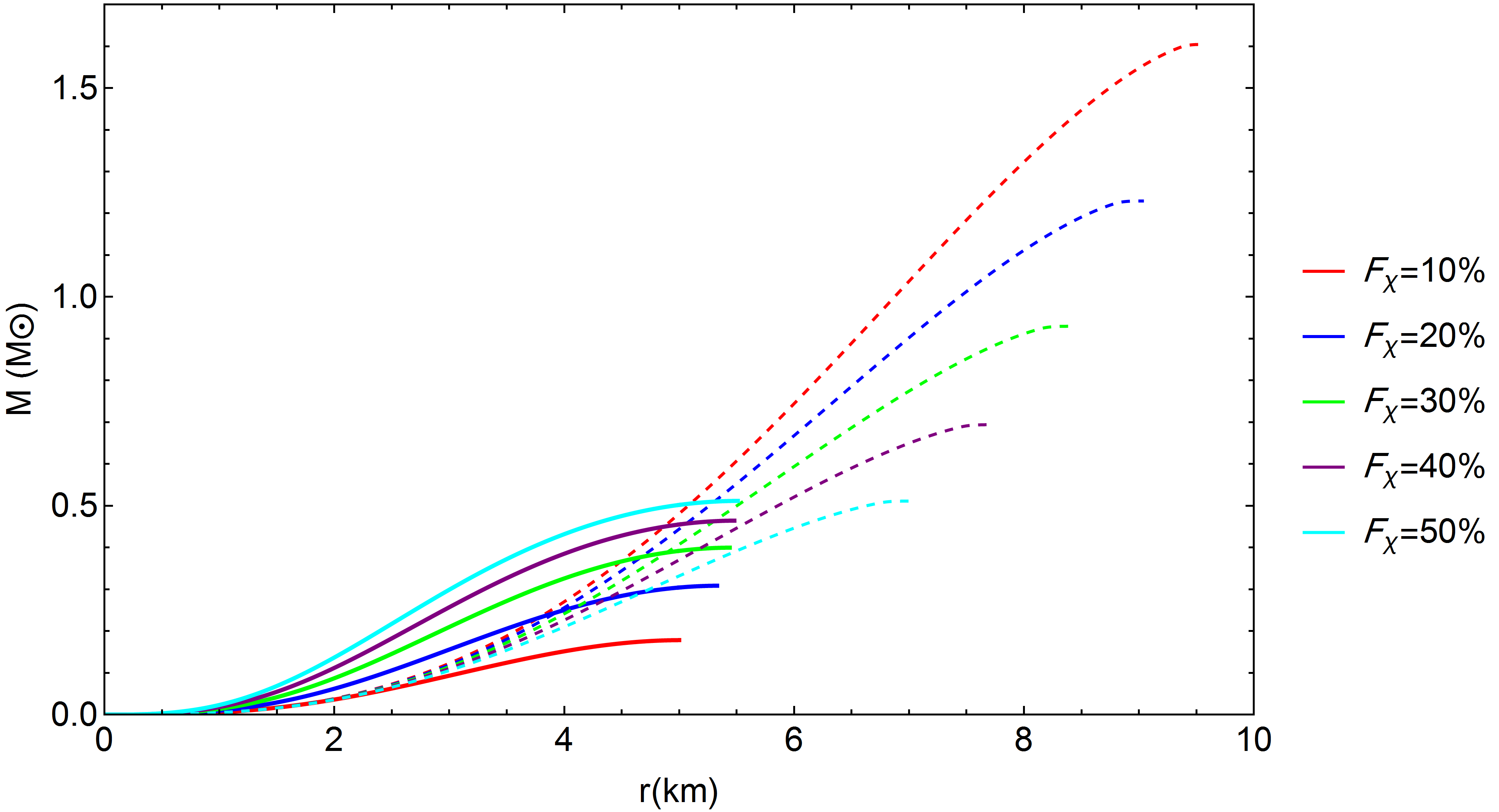
As the distribution of DM depends on the particle’s mass $m_{\chi}$, fraction $F_{\chi}$ and the value of the coupling constant $\lambda$ we perform a thorough analysis to show the role of each parameter. Thus, Fig. 1 shows energy density and mass profiles for $m_{\chi}=400$ MeV, $\lambda=\pi$ values and different DM fractions $F_{\chi}$ between $10\%-50\%$. It was implemented by fixing pressure of both components in the center in such a way to obtain the desired fraction. For better understanding each matter component is depicted separately, i.e, BM (dashed lines) and DM (solid lines). From Fig. 1, we see that a DM core with $R_{D}\approx 5\text{km}$ is embedded in a baryonic star with bigger radius. An increase of DM fraction from $10\%$ to $50\%$ leads to an increase of the size and mass of the DM core, while these properties of baryonic component decrease and it becomes more compact.

Another type of behavior is demonstrated in Fig. 2 where energy density and mass profiles for $m_{\chi}=100$ MeV are presented. As it is seen the light DM particles lead to a formation of a halo around BM star with much larger radius that is a function of DM fraction. Higher fractions lead to an increase of mass and radius of DM halo.

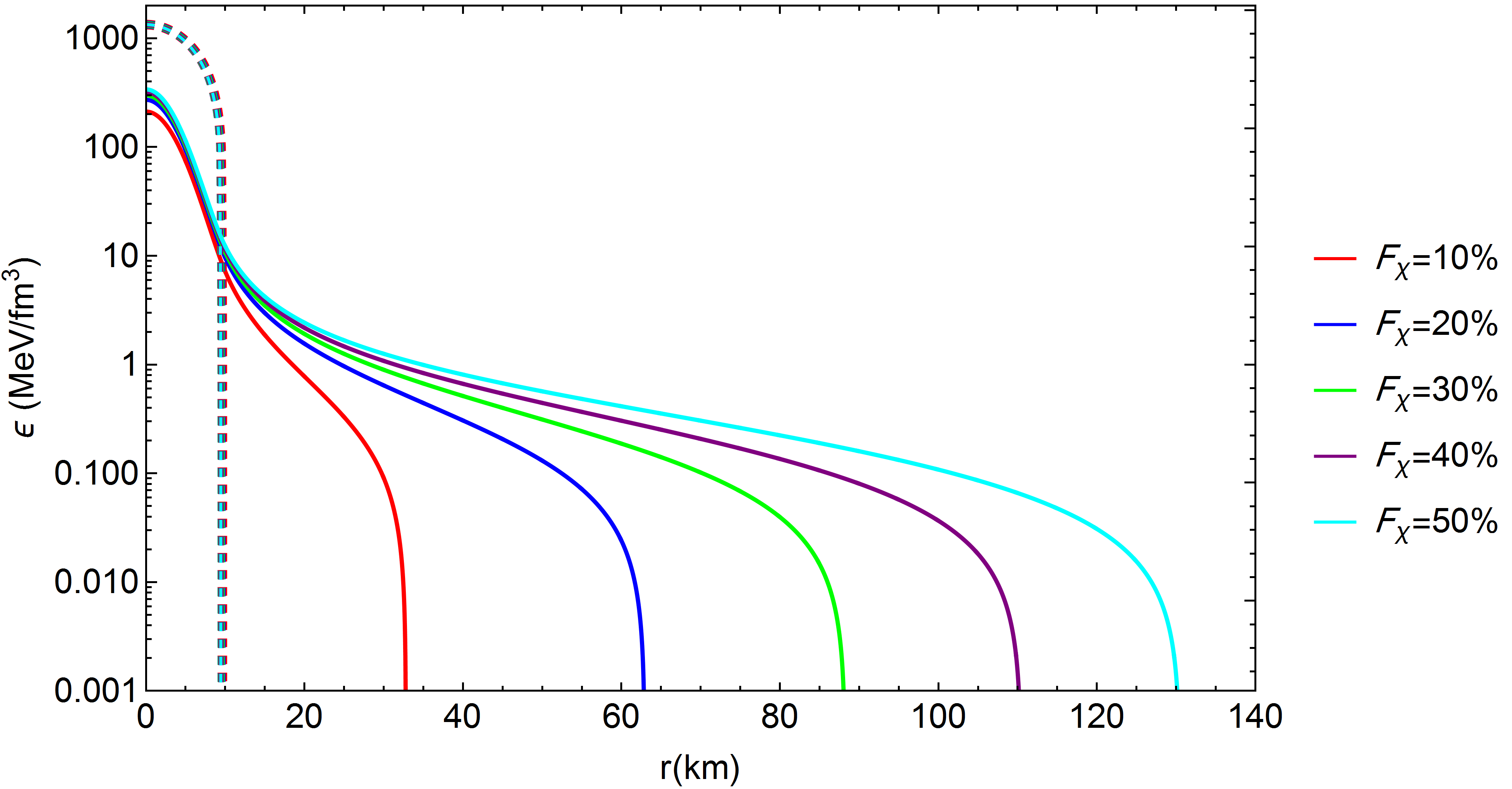
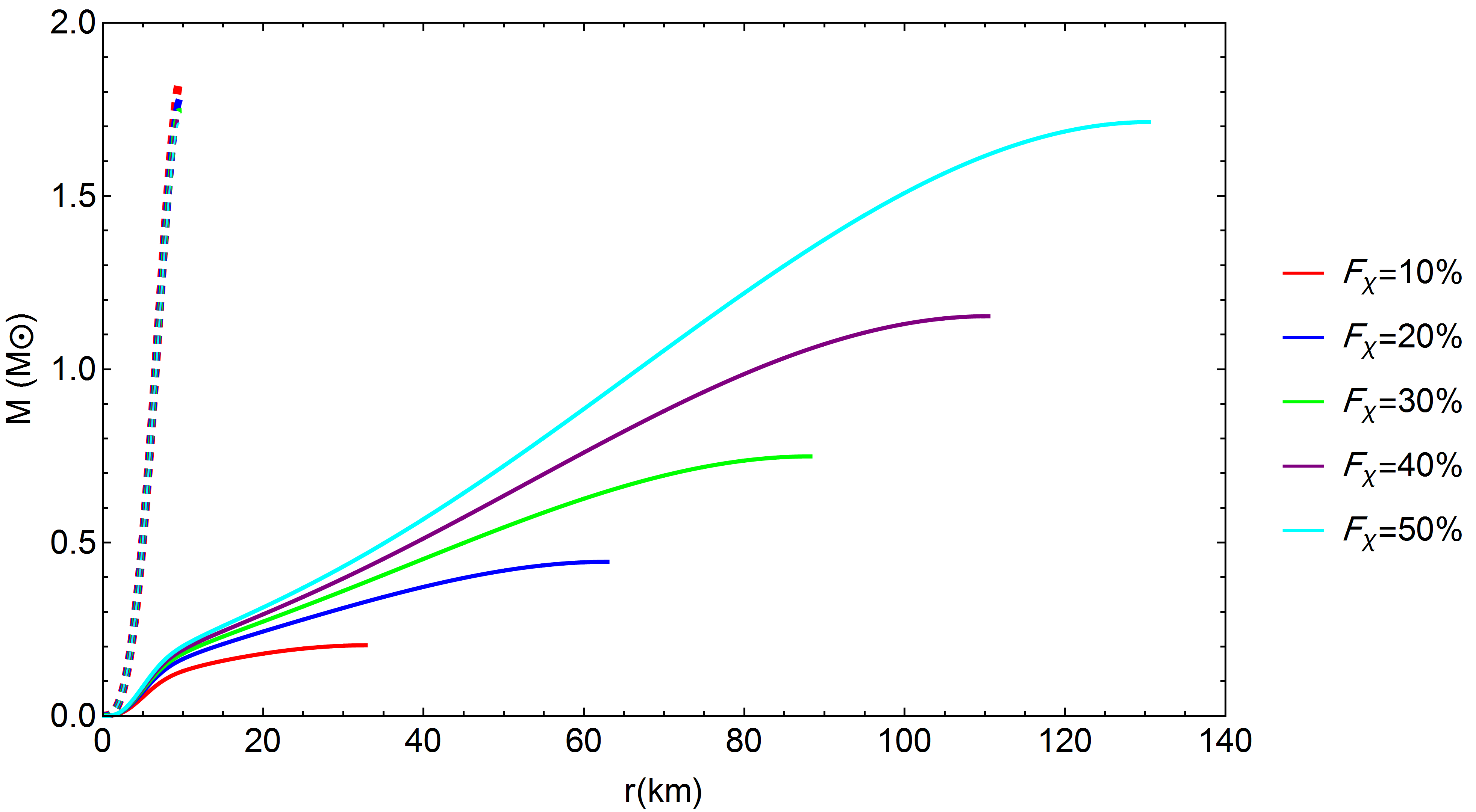
A comparison of Figs. 1 and 2 makes us to conclude that a transition from DM core to halo occurs from $m_{\chi}=400$ MeV to $100$ MeV for $\lambda=\pi$ and different values of $F_{\chi}$. To spot the exact value of $m_{\chi}$ at which this transition happens, we plot the energy density profiles for BM and DM separately with $m_{\chi}$ varies from 100 MeV to 500 MeV at fixed $\lambda$ and $F_{\chi}$. As it is seen on the upper panel of Fig. 3 at $m_{\chi}\approx 175$ MeV radii of both components coincide ($R_{B}\approx R_{D}$), while a slight decrease of $m_{\chi}$ leads to the formation of halo structure with $R_{D}>R_{B}$. In the opposite case, the DM core will be formed for more massive SIDM particles. The middle and lower panels show how the DM distribution is changed by varying the value of coupling constant and DM fraction. By a thorough analysis of an effect of model parameters from Fig. 3, one can show that a DM halo is always formed around NS for $F_{\chi}=10\%$ and $\lambda$ in the range between $0.5\pi-2\pi$ for $m_{\chi}\leq 140$ MeV. A compatible result has been obtained recently in Ref. Ivanytskyi et al. 2020 but for fermionic DM without any self-interaction.

Therefore, as a general behavior we can conclude that light DM particles with $m_{\chi}<200$ MeV tend to form halo around a NS, while heavier ones for low DM fractions would mainly create a DM core inside a compact star. However, for massive DM particles it would be still possible to form a DM halo for high values of $F_{\chi}$. More detailed consideration of the role of DM fraction in the formation of DM core and DM halo will be presented in the following section.

The mass-radius (M-R) relations for DM admixed NSs are shown in Figs. 4 and 5 in which $M=M_{T}=M_{B}+M_{D}$. Here $R$ is the outermost radius of the star which is determined by $R_{B}$ for (i) and (ii) scenarios and by $R_{D}$ for iii) scenario that includes a DM halo formation. A solid black curve on each panel corresponds to the M-R relation for pure baryonic stars described by the IST EoS. Gray dashed horizontal line indicates the $2M_{\odot}$ maximum mass limit for NS, magenta and cyan regions mark causality and GR limits, respectively.

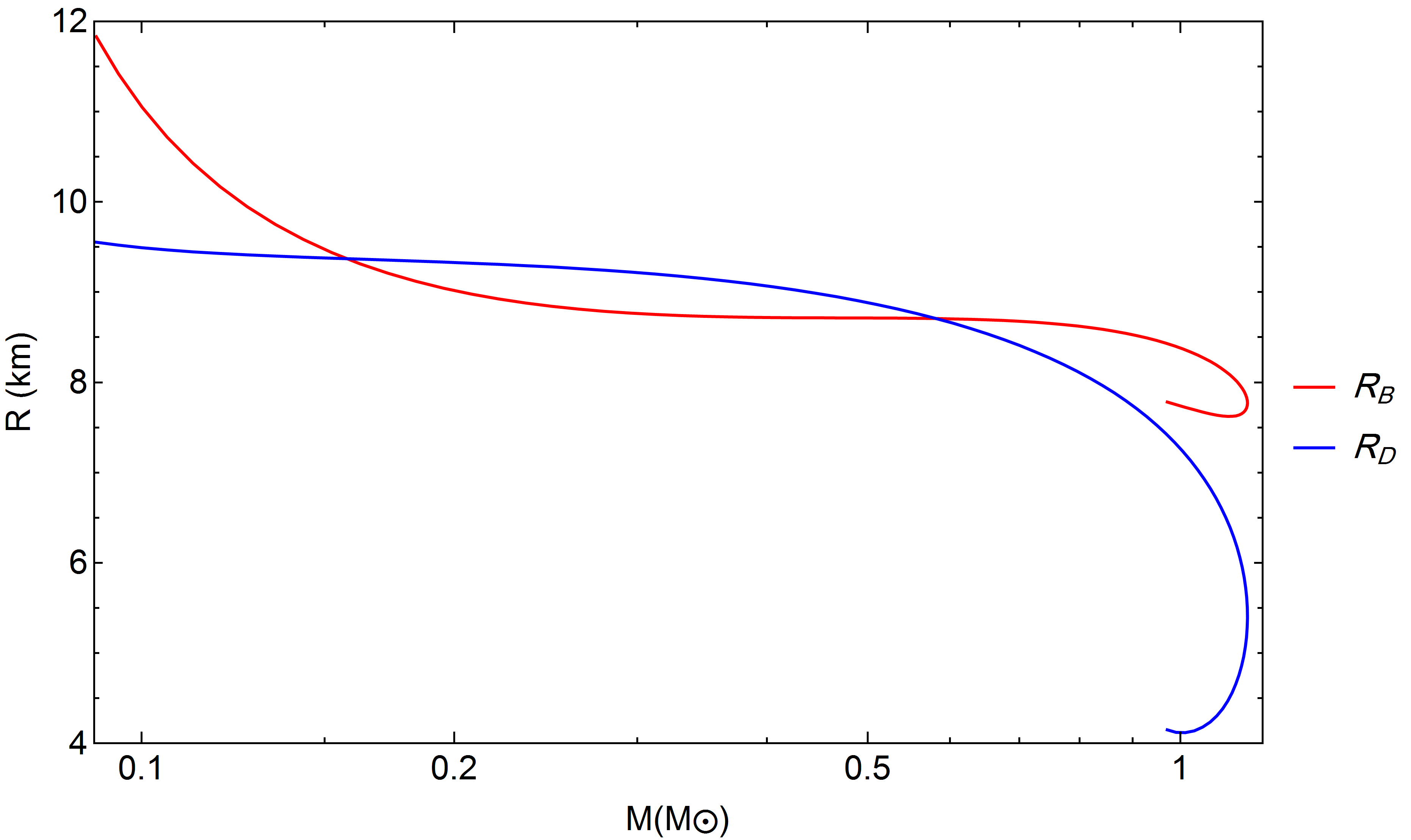
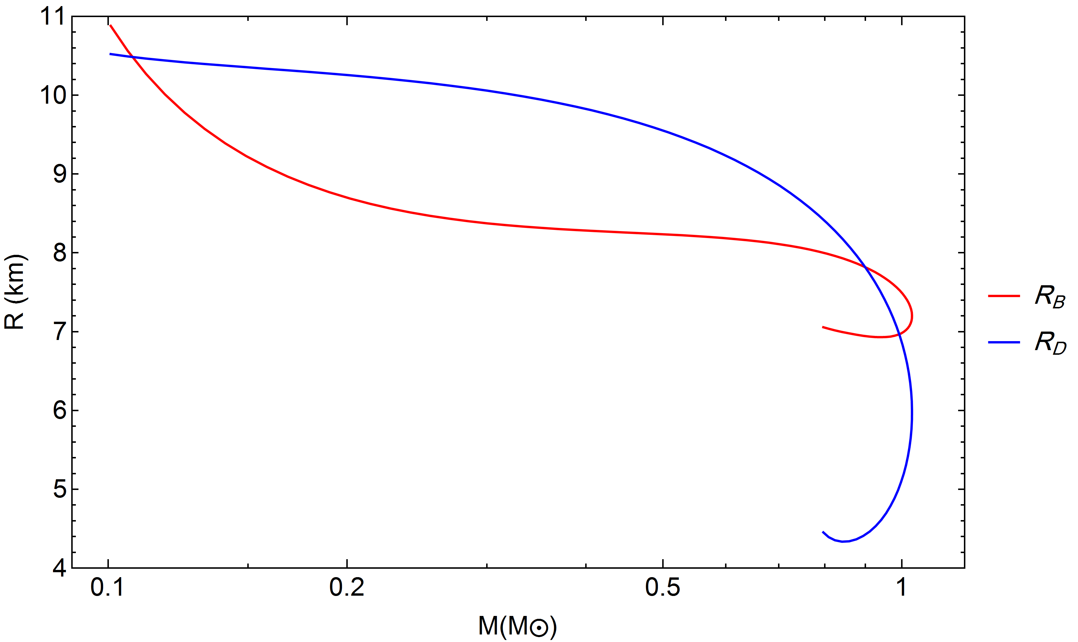
In Fig. 4 we show an effect of different values of $m_{\chi}$ and $\lambda$ on the maximum mass and profile of the M-R relation of DM admixed NSs for a fixed DM fraction $20\%$. In the lower panel, it is shown that a decrease of $m_{\chi}$ leads to an increase of the maximum mass. We find that the star’s radius grows very drastically for lower DM masses compared to heavy masses, due to the fact that the outermost radius of the star in the former case is determined by $R_{D}$ (DM EoS), while the latter one is defined by $R_{B}$ (BM EoS). For $m_{\chi}=100$ MeV (red dashed curve in the lower panel of Fig. 4) for which a DM halo forms around a baryonic NS, the total maximum mass increases. On the other hand for $m_{\chi}>200$ MeV a DM core forms inside a NS leading to a decrease of the total mass compared to a pure BM star. As an intermediate regime, we want to point out on the blue dashed curve in the lower panel of Fig. 4 obtained for $m_{\chi}=200$ MeV, $F_{\chi}=20\%$ and $\lambda=\pi$ which shows a reduction of the maximum mass although a DM halo is formed (see Fig. 11 for more details).

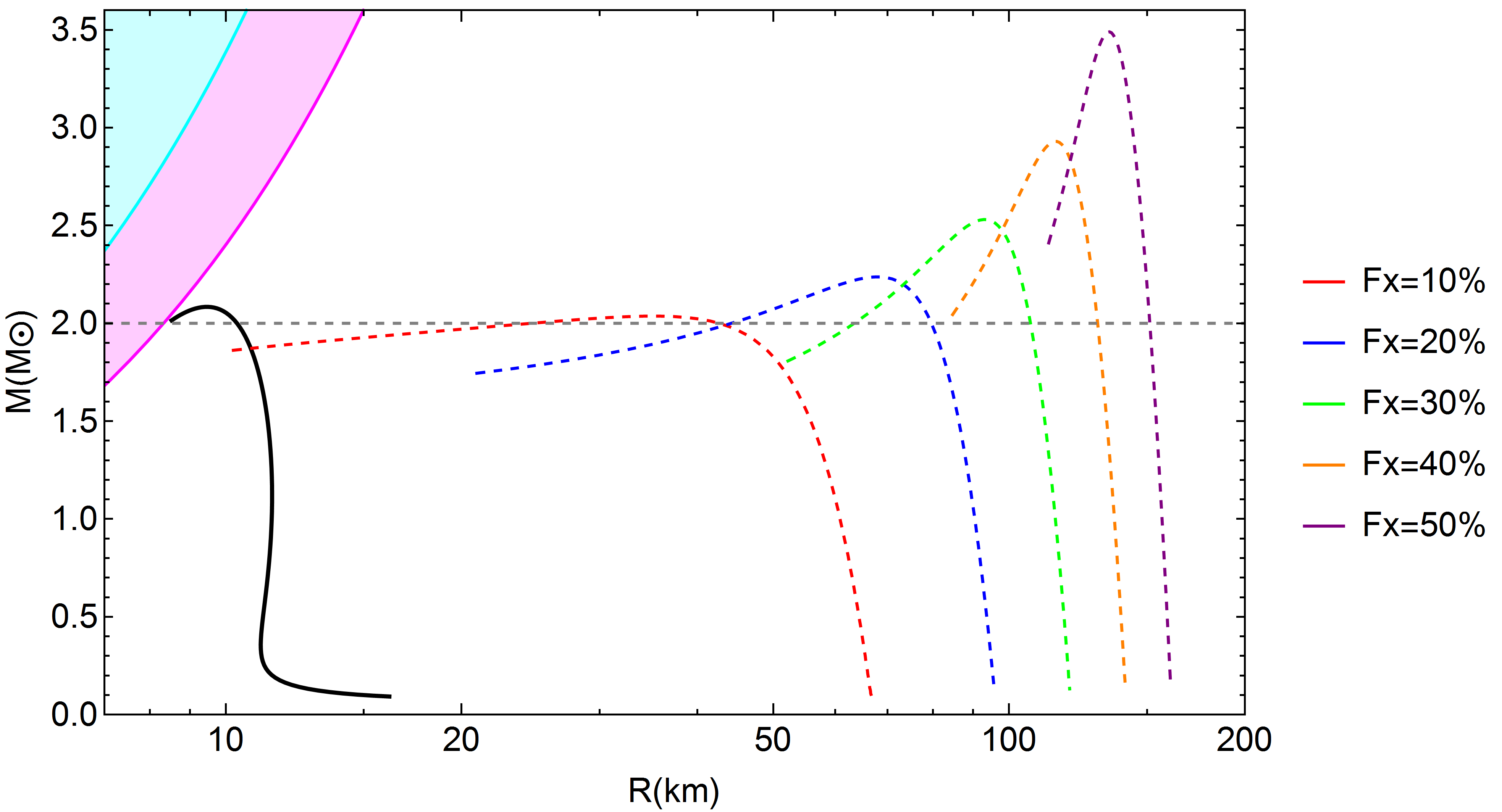
In the upper panel of Fig. 4 an effect of self-coupling constant $\lambda=(0.5,1,1.5,2)\pi$ on the total maximum mass of the compact stars is investigated. Here M-R profiles are shown for $m_{\chi}=100$ MeV (dashed curves) as an example of a DM halo and $m_{\chi}=400$ MeV (solid curves) to illustrate a DM core formation. As you can see on the upper panel of Fig. 4, DM particles with mass $400$ MeV lead to a decrease of the maximum mass leaving it below $2M_{\odot}$ constraint. At the same time, an increase of $\lambda$ rises the maximum mass for both DM masses while the star’s radius has a small reduction for $m_{\chi}=400$ MeV and drastically increases for $m_{\chi}=100$ MeV.

We show an impact of DM fraction on the M-R profiles of compact stars in Fig. 5. For light DM particles with mass $100$ MeV (see the upper panel) the bigger fraction causes a grow of the maximum mass and radius of stars. For heavier DM particles $m_{\chi}=400$ MeV, we see an opposite behavior that prompt a reduction of total maximum mass and radius with an increase of fraction (lower panel on Fig. 5). It is worth mentioning that for all above mentioned cases in which a DM halo is formed ($R_{D}>R_{B}$), the visible radius of a star remains to be $R_{B}$.

We see here that in agreement with previous studies the existence of a DM core decreases the maximum stable mass and the corresponding minimum radius while the formation of a DM halo increases these quantities Leung et al. 2011; Nelson et al. 2019; Ivanytskyi et al. 2020; Ellis et al. 2018a. Moreover, we report a new interesting behavior presented on the lower panel of Fig. 4 for $m_{\chi}=300$ MeV and $F_{\chi}=20\%$ and on the lower panel of Fig. 5 for $m_{\chi}=400$ MeV and $F_{\chi}=40\%$, 50% which occurs due to a DM core - halo transition. In fact, for a given $m_{\chi}$, $\lambda$ and $F_{\chi}$ values the outermost radius of the object may interchange between $R_{B}$ and $R_{D}$ along the M-R profile for DM admixed NSs. To clarify this new interesting feature, we plotted the radius of BM and DM components separately (see Figs. 6-7). Thus, Fig. 6 for $m_{\chi}=300$ MeV (green dashed curve) shows that for an intermediate mass range the radius of the DM component exceeds the BM one, $R_{D}>R_{B}$, while for the low and high mass tails the baryonic component has a larger radius. Fig. 7 illustrates a similar transition for particles with $m_{\chi}=400$ MeV and high DM fractions $40\%$ and $50\%$. Along the M-R relation $R_{D}<R_{B}$ for the low mass stars, $R_{D}>R_{B}$ in the intermediate region of total gravitational masses, and $R_{D}<R_{B}$ for massive stars. According to our best knowledge, this is a new feature never reported before, we named it a DM core - halo transition.

To have a clear understanding on how the results depend on DM model parameters, we present a behavior of the maximum total gravitational mass of DM admixed NSs in a wide range of DM fractions in Fig. 8. This figure shows that considering $\lambda=\pi$, (i) for $m_{\chi}\leq 105$ MeV, the maximum mass is always above $2M_{\odot}$ for any DM fraction. The limiting masses for different self-coupling constants are given as ($\lambda,m_{\chi}$)= ($0.5\pi$, 88.4 MeV), ($1.5\pi$, 116 MeV) and ($2\pi$, 125 MeV). (ii) For a DM mass range between $105$ MeV and $200$ MeV the maximum total mass decreases for low DM fractions, and goes below $2M_{\odot}$. However, by increasing $F_{\chi}$, the maximum total mass after reaching to a local minimum gradually increases above $2M_{\odot}$ for high DM fractions. This behaviour is a signature of a core to halo transition induced by variation of amount of DM fraction. (iii) For bosons with masses of about $m_{\chi}\gtrsim 300$ MeV, we clearly see a DM core formation inside NSs leading to a reduction of the total mass by increasing the DM fraction. For massive DM particles and high fractions, we see a small rise of the total maximum mass, however it never reaches to $2M_{\odot}$ limit even for a pure DM star.

The effect of different values of self-coupling constant $\lambda=(0.5,1,1.5,2)\pi$ on the total maximum mass as a function of DM fraction is depicted in Fig. 9 for $m_{\chi}$=100, 200 and 400 MeV. This figure shows that the total maximum mass grows by increasing $\lambda$ and the DM fraction at which $M_{T_{max}}$ crosses $2M_{\odot}$ line has a strong dependence on $\lambda$. Fig. 10 illustrates a contribution of BM (dashed curves) and DM (dot-dashed curves) components to the maximum total gravitational mass (solid curves) of DM admixed NSs. As you can see, in contrast to $M_{B}$, $M_{D}$ is increasing with $F_{\chi}$, however, the variation rates of these two masses are considerably different for a DM halo (e.g, $m_{\chi}=100$ MeV) and for a DM core (e.g, $m_{\chi}=400$ MeV). We see from Fig. 11 that depending on the DM masses for a fixed $\lambda=\pi$, a DM halo starts to form at a specific fraction of DM when $R_{D}>R_{B}$. The upper panel shows the variation of radii of the DM component $R_{D}$ (dotted curves) and the BM one $R_{B}$ (solid curves) as a function of DM fraction for different $m_{\chi}$. It indicates that $R_{B}\approx 10$ km, while $R_{D}$ gradually increases toward larger values. The condition $R_{D}\approx R_{B}$ satisfies when a DM halo appears. On the lower panel of Fig. 11, the total maximum mass (solid curves), $R_{D}$ (dashed curves) and $R_{B}$ (dotted curves) are presented in a single plot. It can be seen that a DM halo is appeared for $m_{\chi}=100$ MeV, 150 MeV at $F_{\chi}<10\%$ and for $m_{\chi}=200$ MeV at $F_{\chi}<20\%$. However, the total maximum mass of DM admixed NS starts to increase at higher DM fractions compared to the one of halo formation.

In this section, we analyse an effect of bosonic SIDM on the tidal deformability $\Lambda$ of a DM admixed NS. The quadrupole tidal distortion $Q_{ij}$ in terms of external tidal tensor $\mathcal{E}_{ij}$ can be parametrized as follows

$\displaystyle Q_{ij}=\frac{2}{3}k_{2}R^{5}\mathcal{E}_{ij}=\lambda_{t}\mathcal{E}_{ij}\,,$

(14)

where $k_{2}$ is the tidal Love number which can be calculated from the TOV equations Hinderer 2008; Postnikov et al. 2010. Therefore, the tidal deformability $\lambda_{t}$ strongly depends on the star’s EoS.

Unlike $\lambda_{t}$ which has dimension, dimensionless tidal deformability $\Lambda$ can be defined as

$\displaystyle\Lambda=\frac{\lambda_{t}}{M^{5}}=\frac{2}{3}k_{2}\left(\frac{R}{M}\right)^{5}\,.$

(15)

Here R and M are the radius and mass of a compact star, $k_{2}$ is calculated by the method presented in Refs. Hinderer 2008; Hinderer et al. 2010; Postnikov et al. 2010 as

	$\displaystyle k_{2}$	$\displaystyle=$	$\displaystyle\frac{8C^{5}}{5}(1-2C)^{2}[2+2C(y-1)-y]$		(16)
			$\displaystyle\times\{2C[6-3y+3C(5y-8)]$
			$\displaystyle+4C^{3}[13-11y+C(3y-2)$
			$\displaystyle+2C^{2}(1+y)]+3(1-2C)^{2}[2-y$
			$\displaystyle+2C(y-1)]\ln(1-2C)\}^{-1}\,,$

here $C=M/R$ is the compactness and $y$ is related to the quadrupolar perturbed metric function. It is determined at the star’s surface $y\equiv y(r)|_{r=R}$ through solving the following differential equation with the appropriate boundary conditions Hinderer 2008

	$\displaystyle ry^{\prime}(r)+y(r)^{2}+y(r)e^{\lambda(r)}\left\{1+4\pi r^{2}\right.$				(17)
	$\displaystyle\left.\left[p(r)-\epsilon(r)\right]\right\}+r^{2}Q(r)$	$\displaystyle=$	$\displaystyle 0.$

Assuming a spherically symmetric star, the metric functions $\lambda(r)$ and $\nu(r)$ are given by

	$\displaystyle e^{\lambda(r)}$	$\displaystyle=$	$\displaystyle\left[1-\frac{2M(r)}{r}\right]^{-1},$		(18)
	$\displaystyle\frac{d\nu}{dr}$	$\displaystyle=$	$\displaystyle\frac{2}{r}\left[\frac{M(r)+4\pi p(r)r^{3}}{r-2M(r)}\right].$		(19)

By using EoSs for BM and DM as inputs and setting the initial condition $y(0)=2$ Kumar et al. 2017; Postnikov et al. 2010, the values of $y$, $k_{2}$ and $\Lambda$ can be calculated by simultaneously solving the TOV equations and Eq. (17). For a two fluid system composed of DM and BM, the parameters $\epsilon$, $p$ and $M$ are defined as

$\displaystyle p=\sum_{i}p_{i},\ \ \epsilon=\sum_{i}\epsilon_{i},\ \ M=\sum_{i}M_{i},\ \ \text{i=BM, DM}.~~~~~$

(20)

The parameter $Q(r)$ (see Appendix B of Ref. Das et al. 2020b) is given by

	$\displaystyle Q(r)=4\pi e^{\lambda(r)}\left[5\epsilon(r)+9p(r)+\sum_{i}\frac{\epsilon_{i}(r)+p_{i}(r)}{dp_{i}/d\epsilon_{i}}\right]$
	$\displaystyle-6\frac{e^{\lambda(r)}}{r^{2}}-(\nu^{\prime}(r))^{2}.\ ~~$		(21)

Note that in a DM admixed NS, $y$ and $C$ and, therefore, $k_{2}$ should be determined at the outermost radius of the object. In other words, the tidal deformability parameter is sensitive to the gravitational radius which might be different from the visible radius of the star. For a DM halo $R=R_{D}$ and for a DM core $R=R_{B}$. Meanwhile, stiffness and softness of the EoS affects the tidal deformability through $k_{2}$ parameter.

In the following, we investigate the effect of the bosonic SIDM distributed either as a DM core or a DM halo on the dimensionless tidal deformability parameter. The dependence of $\Lambda$ on the total gravitational mass and radius of DM admixed NSs is shown in Figs. 12 -14 for different values of $m_{\chi}$, $\lambda$ and $F_{\chi}$. In these figures the gray horizontal dashed lines indicate the LIGO/Virgo upper bound $\Lambda_{1.4}=580$ Abbott et al. 2018, the gray solid vertical lines show $M_{T}=1.4M_{\odot}$ and the colored dashed vertical lines stand for $R_{1.4}$ radius for the corresponding model parameters.

The tidal deformability calculated for the pure baryonic IST EoS (see Sec. II.2) is denoted by the solid black curve in Figs. 12 -14. As you can see, its $\Lambda_{1.4}$ value is well below the LIGO/Virgo constraint. Thus, within the IST EoS we are able to model both core and halo distributions without violating the tidal deformability constraint. It is related to the fact that the presence of a dense DM core or an extended halo effectively leads to decrease or increase of $\Lambda$, respectively. However for those BM EoSs for which $\Lambda_{1.4}>580$, in order to be compatible with GW170817 tidal limit, the presence of DM mainly as a core component is allowed.

In fact, a general profile of the tidal deformability in Figs. 12 -14 is a decreasing (increasing) function of the total gravitational mass (radius). From Eq. (15), we can see that $\Lambda$ is a function of $R/M$, and, therefore, its lowest value is associated with the maximum mass and/or minimum radius of the DM admixed NS. The main reason that the tidal deformability increases when a DM halo forms around a NS and reduces when a DM core forms inside it, is related to a strong dependence of $\Lambda$ on the stellar radius (the outermost radius) and mass through Eq. (15).

The effect of varying the boson mass $m_{\chi}$ on the tidal deformability is illustrated in Fig. 12 for $\lambda=\pi$ and $F_{\chi}=10\%$. As you can see, a decrease of the DM particle’s mass leads to an increase of $\Lambda$. Such a behavior is in agreement with our understanding, since for light DM particles a DM halo tends to form. It consequently causes a growth of the outermost radius of the object giving rise to higher values of the tidal deformability parameter. On the lower panel of Fig. 12, it is shown how $R_{1.4}$ grows as $m_{\chi}$ becomes smaller. At the same time in the upper panel, the tidal deformability for $m_{\chi}<200$ MeV lies above the curve for the IST EoS (black curve). However, when a DM core is formed inside a NS (e.g, $m_{\chi}\geq 300$ MeV), $\Lambda$ value drops below the one for the IST EoS. Note that a change in the behavior of the tidal deformability curve as a function of R for $m_{\chi}=200$ MeV is an indication of a DM core - halo transition which has been extensively discussed in Sec IV. During a transition the outermost radius of the star switches between $R_{B}$ and $R_{D}$.

Fig. 13 shows how DM fraction affects the tidal deformability of DM admixed NSs at the fixed value of boson mass $m_{\chi}=200$ MeV and $\lambda=\pi$. Higher DM fractions correspond to a DM halo formation leading to higher $\Lambda$ values and $\Lambda_{1.4}\leq 580$ constraint is fulfilled for $F_{\chi}\leq 25\%$. However, low DM fractions give rise to a DM core formation, and, consequently, cause a reduction of the tidal deformability to be below the IST curve. A DM core - halo transition is among the features that appears by changing $F_{\chi}$. In Fig. 14, the tidal deformability is calculated for different values of the self-coupling constant between $0.5\pi$ and $2\pi$ for $m_{\chi}=200$ MeV and $F_{\chi}=10\%$. It turns out that higher values of $\lambda$ generate larger $\Lambda$. Note, that a core-halo transition can be observed for all curves in Fig. 14.

It is important to note that in the case of a DM halo formation for relatively light DM particles with $m_{\chi}\leq 100$ MeV, radius of DM component $R_{D}$ (see Figs. 4 - 5) can reach even above 100 km, which leads to significant enhancement of the value of tidal deformability.

At the moment, an analysis of the inspiral phase of NS-NS coalescence does not include hydrodynamic simulations, and therefore it is limited to a case of finite separation between the stars. To stay in agreement with the present GW analysis, we restrict ourselves to $R_{D}\leq 75$ km to prevent an overlap of DM halos which corresponds to lower frequencies detectable by Ad. LIGO Nelson et al. 2019; Ellis et al. 2018a.

To give more insight, taking into account the observable constraint from GW170817 Abbott et al. 2017; Abbott et al. 2018, in Fig. 15, we demonstrate the tidal deformability as a function of $F_{\chi}$ for a fixed value of the total star’s mass $1.4M_{\odot}$. On the upper panel, the tidal deformability is an increasing function of DM fraction for the light DM particles where a DM halo is formed for $F_{\chi}\leq 6\%$. The horizontal gray line indicates $F_{\chi}$ at which a DM admixed NS satisfies the $\Lambda_{1.4}\leq 580$ constraint. On the middle panel, we consider an intermediate mass range between 200 MeV - 230 MeV for which the tidal deformability behavior shows the features of both a DM core (part of the curve depicted as dashed) and a DM halo (part of the curve depicted as solid). We see that for low DM fractions $F_{\chi}\leq 10\%$, DM tends to condensate in the core of a NS and $\Lambda$ is a decreasing function of $F_{\chi}$. The tidal deformability reaches minimum at a specific value of DM fraction at which a core to halo transition occurs and afterwards $\Lambda$ starts to grow with $F_{\chi}$.

On the lower panel of Fig. 15, we show three curves calculated for $m_{\chi}=(300,400,500$) MeV that tend to create a dense DM core inside a NS. In this case the tidal deformability is a monotonically decreasing function, which heavier DM particles cause bigger reduction in $\Lambda$ at a fixed fraction. Regarding the tidal deformability of NSs admixed with heavy DM particles, we should be careful about the lower tidal limit reported by LIGO/Virgo Collaborations to be $\Lambda_{1.4}=70$ Abbott et al. 2018. Meanwhile, according to the recent results of NICER Miller et al. 2019; Raaijmakers et al. 2020; Miller et al. 2021 and astrophysical observations Özel and Freire 2016; Raaijmakers et al. 2021, we know that $R_{1.4}$ is about 12 km, this is an additional reason for cutting the DM core curves at a specific DM fraction.

Finally, for the sake of completeness, the effect of DM self-interaction strength $\lambda$ for $m_{\chi}=100$ MeV (upper panel) and $m_{\chi}=400$ MeV (lower panel) for $1.4M_{\odot}$ star is presented in Fig. 16. It turns out that for higher values of the coupling constant an allowed range of DM fractions, consistent with $\Lambda_{1.4}\leq 580$ constraint, is decreased (see the upper panel of Fig. 16). The lower panel shows that higher $\lambda$ leads to higher tidal deformability for a fixed DM fraction. In fact the DM EoS for the higher coupling constants is stiffer which causes larger values of the tidal deformability. Thus, regardless of the DM being distributed in a core or a halo, higher values of $\lambda$ leads to larger $\Lambda$ at fixed $F_{\chi}$ for DM admixed NSs.

In summary, we show that in agreement with the previous studies the DM halo causes an increase of the tidal deformability Nelson et al. 2019, while the DM core reduces the tidal deformability compared to the case of pure BM Ellis et al. 2018a. Interestingly for the first time we show that there is a continues transition between a DM core and a DM halo regimes for different DM masses and fractions. In fact depending on the DM fraction, particles of different masses in sub-GeV range can form either a DM core or a DM halo, as was shown previously in Fig. 11. The light bosons $m_{\chi}\lesssim 200$ MeV form a DM core at very small fractions and DM halo at intermediate and large fractions while heavy bosons $m_{\chi}\gtrsim 300$ MeV lead to a DM halo at very large values of $F_{\chi}$ and a DM core at intermediate and small $F_{\chi}$.

As it was shown in the Secs. III-V, the properties of DM admixed NSs depend on three model parameters: boson mass $m_{\chi}$, DM fraction $F_{\chi}$ and the value of the coupling constant $\lambda$. To make the final conclusion about the allowed range of parameters in a 2D plot, we fixed $\lambda=\pi$ as the medium and most representative value of the coupling constant in our consideration. In Fig. 17, the remaining two parameters are plotted with an indication of the total maximum mass and the tidal deformability values. The solid black curve in Fig. 17 indicates the values of $F_{\chi}$ and $m_{\chi}$ for which the total maximum gravitational mass equals to $M_{T_{max}}=2M_{{\odot}}$. Thus, any point below the black curve (cyan region in Fig. 17) gives $M_{T_{max}}>2M_{{\odot}}$ which is in agreement with the two heaviest observed pulsars Antoniadis et al. 2013; Cromartie et al. 2019. The dark red curve depicts the tidal deformability constraint $\Lambda_{1.4}=580$ Abbott et al. 2018. Hence, all the parameter space on the right hand side of the red line (dark red region in Fig. 17) yields $\Lambda_{1.4}\leq 580$ values. Note that in a log scale the $\Lambda_{1.4}=580$ constraint is a straight line. A DM core formation constraints an upper limit of the allowed range of parameters due to decrease of the maximum mass of DM admixed NS for $m_{\chi}>200$ MeV and $F_{\chi}\lesssim 10\%$. However, lighter bosons that form a DM halo around a NS impose a lower limit on the allowed range of parameters, since a DM halo increases the tidal deformability and could exceed the limit reported by the LIGO/Virgo Collaboration.

From Fig. 17, we see that allowed DM fractions inside NS drastically narrowed down by inclusion the tidal deformability constraint, more specifically for $m_{\chi}\lesssim 70$ MeV it imposes a limit on the amount of DM to be less than $1\%$ of the total NS mass. We can conclude that for sub-GeV bosonic DM, the existing observational data support low DM fractions below $5\%$. According to our study, the recent measurements for the maximum mass and tidal deformability of NSs are in agreement with the DM admixed NS scenario. The fraction of DM in their interior is compatible with the amount accreted during star’s lifetime as well as its possible augmentation that will be discussed in Sec. VII. By applying two observable quantities we set a stringent constraint on the amount of DM inside NSs. Further narrowing down the DM fractions is possible by considering simultaneous measurements of mass and radius, e.g, by ongoing NICER observations Riley et al. 2021; Miller et al. 2021; Raaijmakers et al. 2021.

It is worth mentioning that Fig. 17 shows the results for one value of the coupling constant $\lambda=\pi$. For the higher values of $\lambda$ the $M_{T_{max}}=2M_{\odot}$ curve will be lifted up, increasing the range of fractions compatible with the heaviest observed NSs. On the other hand, the $\Lambda_{1.4}=580$ curve will be shifted to the right, limiting the allowed values of $F_{\chi}$ consistent with the LIGO/Virgo constraint. A detailed analysis of the above mentioned effects and a scan over different values of the coupling constants will be subject of a following paper.

An important question we want to address at this section is related to how compact stars can contain and accumulate DM in their interior. The capturing rate of DM by NSs depends on the local density of DM, the DM-BM scattering cross section, and the DM mass Bramante et al. 2013; Bell et al. 2021; Bell et al. 2020. If the DM decay or annihilation is permitted, the number of DM particles in a NS could be depleted. The most plausible scenario for the presence of DM in NSs is its accumulation throughout different stages of star’s lifetime. In this regard, four main evolution phases should be considered: (a) progenitor, (b) main sequence star, (c) supernova explosion with formation of a proto-NS, and (d) equilibrated NS. Depending on the distance of a star from the Galactic center the local DM density varies significantly, and consequently the amount of accreted DM Navarro et al. 1996; Einasto 1965; Ruffini et al. 2015; Argüelles et al. 2018; Del Popolo et al. 2020; Ivanytskyi et al. 2020; Ciancarella et al. 2021. The total accreted mass in a spherically symmetric accretion scenario for a typical NS with $M=1.4M_{\odot}$ and $R=10$ km is given by

$$M_{acc}\approx 10^{-14}\left(\frac{\rho_{dm}}{0.3\ GeV/cm^{3}}\right)\left(\frac{\sigma_{\chi n}}{10^{-45}cm^{2}}\right)\left(\frac{t}{Gyr}\right)M_{\odot},$$

(22)

where $\rho_{dm}$ is the local density of DM, $\sigma_{\chi n}$ is the nucleon-DM elastic cross section and t denotes the age of the NS Kouvaris and Tinyakov 2010; Kouvaris 2013. While the DM density in the Solar system is about $0.3$ GeV$/$cm³, it can reach at most $\sim(10^{11}-10^{12})~$GeV$/$cm³ near the center of the Galaxy for certain DM profiles Bertone and Merritt 2005; Merritt 2004; Freese et al. 2009. It can be shown that the accreted mass can be varied from $\sim 10^{-13}-10^{-14}M_{\odot}$ to $\sim 10^{-5}-10^{-8}M_{\odot}$ Ivanytskyi et al. 2020; Del Popolo et al. 2020; Baryakhtar et al. 2017; Bramante and Elahi 2015; Güver et al. 2014. Moreover, DM production in the NS interior might be an additional effective mechanism which should be taken into account. For instance, due to high baryon density in the core of compact stars, during a supernova explosion or a binary NSs merger a creation of DM particles from nucleons could be triggered, whereas a major part of DM could be created and trapped inside a NS Nelson et al. 2019; Ellis et al. 2018a. High DM fractions Li et al. 2012c; Leung et al. 2011; Leung et al. 2012; Ciancarella et al. 2021; Ciarcelluti and Sandin 2011; Sandin and Ciarcelluti 2009 cannot be easily obtained during a typical star’s lifetime from normal accretion processes considering only a smooth spatial distribution of DM in the Galaxy. However, high DM factions inside compact stars can be acquired by accounting for additional scenarios: (i) clumps of DM were present at the early stages of the Universe forming seeds/accretion centers for BM, this process may lead to a DM admixed NS even with dominant contribution of DM. In fact, instead of accretion of DM onto ordinary NS, one may assume accretion of ordinary matter onto a pre-existing dark core Ellis et al. 2018a; Goldman et al. 2013; Ciarcelluti and Sandin 2011; Deliyergiyev et al. 2019. (ii) Since the density of DM at a certain distance from the Galactic center in a first approximation is homogeneous, a NS can pass through a region in space with locally high DM density leading to an accretion of a large amount of DM Sandin and Ciarcelluti 2009; Del Popolo et al. 2020; Deliyergiyev et al. 2019; Li et al. 2012a; Del Popolo et al. 2020; Profumo et al. 2006; Berezinsky et al. 2013; Berezinsky et al. 2014. (iii) One might speculate a formation of a stable compact object composed of ADM as a dark star Kouvaris and Nielsen 2015b; Maselli et al. 2017; Eby et al. 2016. Hence, NS could capture DM from the dark star companion Ellis et al. 2018a; Goldman et al. 2013; Xiang et al. 2014 or a merger like event may occur Ciarcelluti and Sandin 2011; Gresham and Zurek 2019; Sandin and Ciarcelluti 2009. Regarding all above three possible scenarios, we showed that the existence of high DM fractions is tightly constrain by joint observations of the tidal deformability and the maximum mass.

In this paper, we have investigated the possible effects of bosonic ADM with repulsive self-interaction on the compact star properties including its radius and gravitational mass. We have shown that depending on DM model parameters such as boson mass $m_{\chi}$, self-coupling constant $\lambda$ and DM fraction $F_{\chi}$, DM can be distributed either in a core or a halo. The impact of various DM distribution regimes on observable quantities e.g, the maximum total gravitational mass and the tidal deformability has been considered. We found that DM condensed in the core of a NS leads to decrease of the total gravitational mass, radius and the tidal deformability compared to a typical baryonic NS. On the other hand, the presence of DM particles in the halo around the NS increases those observable quantities. A rich phenomenology of the scenario presented in this article allows a transition between the DM core and halo for different particle’s masses and fractions. During the DM core - halo transition, the outermost radius of the object interchanges from the radius of BM to DM component. This leads to some new features in mass-radius profile and the tidal deformability-radius behavior of the DM admixed NS.

As our main result, we show a combined analysis of the observational data for the heaviest observed NSs and the upper bound on the tidal deformability, in order to put a stringent constraint on the DM fraction for sub-GeV bosonic particles (see Fig. 17). We see that allowed region in which both the total maximum mass $M_{T_{max}}\geq 2M_{\odot}$ and tidal deformability $\Lambda_{1.4}\leq 580$ constraints are satisfied is limited to relatively low DM fractions $F_{\chi}\lesssim 5\%$ at the fixed value of the self-coupling constant $\lambda=\pi$.

The upper limit for the allowed DM fraction reduces significantly for light bosons going well below $1\%$. In our study we explore not only the conservative range of fractions achieved by accretion, but also alternative scenarios that predict large amount of DM inside a star. We showed that the existing data on compact stars do not contradict to the DM admixed NS scenario, and every observed NS could potentially contain low DM fraction distributed in a core or in an extended halo. Moreover, DM admixed NS can serve as a satisfactory explanation for the unusual observational evidences on compact stars, e.g, the secondary object in the GW190814 event with the mass about $2.6M_{\odot}$ Abbott et al. 2020b.

Note that for sub-GeV boson masses depending on the DM fraction, formation of both DM core and halo are possible for fixed $m_{\chi}$ and $\lambda$. In order to break the degeneracy and answer the question whether DM exists in the form of halo or core inside NSs, additional observable quantities other than the tidal deformability and the maximum mass are essential. The ongoing observations by the NICER Raaijmakers et al. 2021; Watts 2019; Riley et al. 2021; Miller et al. 2021 and LIGO/Virgo/KAGRA Collaboration Abbott et al. 2021; Abbott et al. 2020b; Akutsu et al. 2020; Akutsu et al. 2019, as well as the future Advanced Telescope for High Energy Astrophysics (ATHENA) Barcons et al. 2012; Cassano et al. 2018, the enhanced X-ray Timing and Polarimetry mission (eXTP) in ’t Zand et al. 2019; Zhang et al. 2019; Zhang et al. 2016, and the Spectroscopic Time-Resolving Observatory for Broadband Energy X-rays (STROBE-X) Ray et al. 2019; Wilson-Hodge et al. 2017 telescopes may shed more light on the possible forms of bosonic SIDM in NSs.

The outermost radius of a compact star with DM condensed in its core equals to the baryonic radius. However, observation of the outermost radius in the case of a DM halo formation imposes much bigger challenges. Due to the fact that DM component distributed in the halo is undetectable through the spectroscopic measurements, the use of multimessenger astronomy is unavoidable. Thus, combining analysis of astrophysical and GW observations, as well as searches for microlensing or other gravitational effects close to the surface of compact stars, may give information about the halo structure around them.

Moreover, an additional piece of valuable data is expected from the radio telescopes, e.g, the Karoo Array Telescope (MeerKAT) Bailes et al. 2018, the Square Kilometer Array (SKA) Watts et al. 2015; Weltman et al. 2020, and the Next Generation Very Large Array (ngVLA) Di Francesco et al. 2019; Selina 2018, that will look into the Galactic center. Despite a big dust extinction in the most central part of the Galaxy, we expect to find pulsars and magnetars in the region up to 70 pc from the center. This region may contain a high DM fraction, and therefore, can host DM admixed compact stars with altered properties.

S.S. and D.R. are very thankful to Fazlollah Hajkarim for insightful discussions and comments on the draft. D.R. appreciates Sajad Khalili for his valuable assistance in writing the codes. V.S. acknowledges the support from the Fundação para a Ciência e  a Tecnologia (FCT) within the projects No. UID/FIS/04564/2019, No. UID/04564/2020 and PHAROS COST Action CA16214. O.I. acknowledges the support from the Polish National Science Centre (NCN) under grant No. 2019/33/B/ST9/03059. It is part of a project that has received funding from the European Union’s Horizon 2020 research and innovation program under grant agreement STRONG – 2020 - No 824093.

The DM EoS (1) has been originally obtained by Colpi et al. 1986. For the readers convenience we present its derivation in a flat space-time. Such a treatment is justified by the fact that gradients of metrics are small compared to the spatial scales. This can be shown by considering the gradient of the time-time component $g_{tt}$. Using the explicit expression from Ref. Oppenheimer and Volkoff 1939 one gets

$\displaystyle\frac{\partial g_{tt}}{\partial r}=-\frac{2g_{tt}}{P+\rho}\frac{dP}{dr}$

(A.1)

with $P$ and $\rho$ being local pressure and energy density. We consider this quantity on the stellar surface where space-time is the most curved. In this case $g_{tt}=1-\frac{2M_{tot}}{R}$, $P=0$ and gradient of the pressure can be expressed using the TOV equation as $\frac{dP}{dr}=-\frac{\rho M_{tot}}{R^{2}g_{tt}}$. This yields $\frac{\partial g_{tt}}{\partial r}=\frac{2M_{tot}}{R^{2}}<\frac{1}{R}$, where the Schwarzschild limit $\frac{2M_{tot}}{R}=1$ was used on the second step. Thus, for a NS of radius $R\sim 10~km$ within the spherical layer of thickness $\Delta r\sim 1~m$, which is enough to be treated as a macroscopical scale allowing thermodynamic treatment of DM, relative deviation of the metrics from the flat one can be estimated as $\Delta r\frac{dg_{tt}}{dr}\lesssim\frac{\Delta r}{R}\sim 10^{-4}$.

The model of bosonic SIDM used in this work corresponds to the Lagrangian

$\displaystyle\mathcal{L}=\frac{1}{2}\partial_{\mu}\phi^{*}\partial^{\mu}\phi-\frac{m_{\chi}^{2}}{2}\phi^{*}\phi-\frac{\lambda}{4}(\phi^{*}\phi)^{2}.$

(A.2)

Under the mean-field approximation deviation of the field bilinear $\phi^{*}\phi$ from its expectation value $\langle\phi^{*}\phi\rangle$ is assumed to be small. Therefore interaction term in $\mathcal{L}$ can be expanded up to terms linear in $\phi^{*}\phi-\langle\phi^{*}\phi\rangle$. Thus, the linearized mean-field Lagrangian becomes

$\displaystyle\mathcal{L}_{MF}=\frac{1}{2}\partial_{\mu}\phi^{*}\partial^{\mu}\phi-\frac{m_{\chi}^{*2}}{2}\phi^{*}\phi+\frac{\lambda}{4}\langle\phi^{*}\phi\rangle^{2}.$

(A.3)

First two terms of this Lagrangian describe free quasiparticles with the effective mass $m_{\chi}^{*2}=m_{\chi}^{2}+\lambda\langle\phi^{*}\phi\rangle$. At zero temperature they form BEC (see e.g, Kapusta and Gale 2011). The corresponding contribution to the total pressure is $\zeta^{2}(\mu^{2}_{\chi}-m_{\chi}^{*2})$, where $\zeta$ represents the amplitude of zero mode and $\mu_{\chi}$ is bosonic chemical potential. The last term in the mean-field Lagrangian does not include any dynamical fields but only the average of their product. Consequently, this term contributes the total pressure just as a constant term. Thus

$\displaystyle P=\zeta^{2}(\mu_{\chi}^{2}-m_{\chi}^{*2})+\frac{\lambda}{4}\langle\phi^{*}\phi\rangle^{2}.$

(A.4)

The amplitude of zero bosonic mode $\zeta$ attains a value, which maximizes the total pressure, i.e, $\frac{\partial p}{\partial\zeta}=0$. Condensate $\langle\phi^{*}\phi\rangle$ also maximizes the pressure leading to the condition $\frac{\partial p}{\partial\langle\phi^{*}\phi\rangle}=0$. Finally, number density of bosons can be defined using the thermodynamic identity $n_{\chi}=\frac{\partial P}{\partial\mu_{\chi}}$. This leads to

	$\displaystyle 2\zeta(\mu_{\chi}^{2}-m_{\chi}^{*2})=0,$		(A.5)
	$\displaystyle\lambda\left(-\zeta^{2}+\frac{\langle\phi^{*}\phi\rangle}{2}\right)=0,$		(A.6)
	$\displaystyle n_{\chi}=2\zeta^{2}\mu_{\chi}.$		(A.7)

Eqs. (A.6) and (A.7) immediately yield $\zeta^{2}=\frac{\langle\phi^{*}\phi\rangle}{2}$ and $n_{\chi}=\langle\phi^{*}\phi\rangle\mu_{\chi}$. Since $\zeta\neq 0$ in the condensate, then Eq. (A.5) gives $\mu_{\chi}^{2}=m_{\chi}^{*2}$ or equivalently $\mu^{2}_{\chi}=m_{\chi}^{2}+\lambda\langle\phi^{*}\phi\rangle$. This defines $\langle\phi^{*}\phi\rangle=\frac{\mu_{\chi}^{2}-m_{\chi}^{2}}{\lambda}$. Consequently, total pressure and DM particle number density become

	$\displaystyle P$	$\displaystyle=$	$\displaystyle\frac{1}{4\lambda}\left(\mu_{\chi}^{2}-m_{\chi}^{2}\right)^{2},$		(A.8)
	$\displaystyle n_{\chi}$	$\displaystyle=$	$\displaystyle\frac{\mu_{\chi}}{\lambda}\left(\mu_{\chi}^{2}-m_{\chi}^{2}\right).$		(A.9)

Energy density can be found using the thermodynamic identity

	$\displaystyle\rho$	$\displaystyle=$	$\displaystyle\mu_{\chi}n_{\chi}-P=\frac{3}{4\lambda}\left(\mu_{\chi}^{2}-m_{\chi}^{2}\right)^{2}+\frac{m_{\chi}^{2}}{\lambda}\left(\mu_{\chi}^{2}-m_{\chi}^{2}\right)$		(A.10)
		$\displaystyle=$	$\displaystyle 3P+2m_{\chi}^{2}\sqrt{\frac{P}{\lambda}},$

where on the second step $\mu_{\chi}^{2}-m_{\chi}^{2}$ was expressed through the pressure. This is a quadratic equation with respect to $\sqrt{P}$ yielding to

$$\sqrt{P}=\frac{1}{3}\left[-\frac{m_{\chi}^{2}}{\sqrt{\lambda}}\pm\sqrt{\left(\frac{m_{\chi}^{2}}{\sqrt{\lambda}}\right)^{2}+3\rho}\right].$$

(A.11)

The sign $"+"$ should be taken in order to provide positiveness of the solution. This gives exactly the Eq. (1).

References

- Bertone and Tait (2018) G. Bertone and T. Tait, M. P., Nature 562, 51 (2018), arXiv:1810.01668 [astro-ph.CO] .
- Bertone and Hooper (2018) G. Bertone and D. Hooper, Rev. Mod. Phys. 90, 045002 (2018), arXiv:1605.04909 [astro-ph.CO] .
- Mayet et al. (2016) F. Mayet et al., Phys. Rept. 627, 1 (2016), arXiv:1602.03781 [astro-ph.CO] .
- Billard et al. (2021) J. Billard et al., (2021), arXiv:2104.07634 [hep-ex] .
- Roberts and Flambaum (2019) B. M. Roberts and V. V. Flambaum, Phys. Rev. D 100, 063017 (2019), arXiv:1904.07127 [hep-ph] .
- Catena et al. (2020) R. Catena, T. Emken, N. A. Spaldin, and W. Tarantino, Phys. Rev. Res. 2, 033195 (2020), arXiv:1912.08204 [hep-ph] .
- Kouvaris and Pradler (2017) C. Kouvaris and J. Pradler, Phys. Rev. Lett. 118, 031803 (2017).
- Essig et al. (2019) R. Essig, J. Pérez-Ríos, H. Ramani, and O. Slone, Phys. Rev. Research 1, 033105 (2019).
- Aprile et al. (2019) E. Aprile et al. (XENON), Phys. Rev. Lett. 123, 251801 (2019), arXiv:1907.11485 [hep-ex] .
- Essig et al. (2017) R. Essig, T. Volansky, and T.-T. Yu, Phys. Rev. D 96, 043017 (2017), arXiv:1703.00910 [hep-ph] .
- Aprile et al. (2020) E. Aprile et al. (XENON), Phys. Rev. D 102, 072004 (2020), arXiv:2006.09721 [hep-ex] .
- Shakeri et al. (2020) S. Shakeri, F. Hajkarim, and S.-S. Xue, JHEP 12, 194 (2020), arXiv:2008.05029 [hep-ph] .
- Cerdeño et al. (2019) D. G. Cerdeño, A. Cheek, P. Martín-Ramiro, and J. M. Moreno, European Physical Journal C 79, 517 (2019), arXiv:1902.01789 [hep-ph] .
- Argüelles et al. (2019) C. A. Argüelles, A. Diaz, A. Kheirandish, A. Olivares-Del-Campo, I. Safa, and A. C. Vincent, arXiv e-prints , arXiv:1912.09486 (2019), arXiv:1912.09486 [hep-ph] .
- Slatyer (2016) T. R. Slatyer, Phys. Rev. D 93, 023521 (2016), arXiv:1506.03812 [astro-ph.CO] .
- Brdar et al. (2018) V. Brdar, J. Kopp, J. Liu, and X.-P. Wang, Phys. Rev. Lett. 120, 061301 (2018), arXiv:1710.02146 [hep-ph] .
- Panotopoulos and Lopes (2017) G. Panotopoulos and I. Lopes, Physical Review D 96 (2017), 10.1103/physrevd.96.083004.
- Nelson et al. (2019) A. E. Nelson, S. Reddy, and D. Zhou, Journal of Cosmology and Astroparticle Physics 2019, 012–012 (2019).
- Ellis et al. (2018a) J. Ellis, G. Hütsi, K. Kannike, L. Marzola, M. Raidal, and V. Vaskonen, Phys. Rev. D 97, 123007 (2018a), arXiv:1804.01418 [astro-ph.CO] .
- Ivanytskyi et al. (2020) O. Ivanytskyi, V. Sagun, and I. Lopes, Phys. Rev. D 102, 063028 (2020).
- Rezaei (2017) Z. Rezaei, Astrophys. J. 835, 33 (2017), arXiv:1612.02804 [astro-ph.HE] .
- de Lavallaz and Fairbairn (2010) A. de Lavallaz and M. Fairbairn, Phys. Rev. D 81, 123521 (2010), arXiv:1004.0629 [astro-ph.GA] .
- Gresham and Zurek (2019) M. I. Gresham and K. M. Zurek, Phys. Rev. D 99, 083008 (2019), arXiv:1809.08254 [astro-ph.CO] .
- Kouvaris (2008) C. Kouvaris, Physical Review D 77 (2008), 10.1103/physrevd.77.023006.
- Bhat and Paul (2020) S. A. Bhat and A. Paul, Eur. Phys. J. C 80, 544 (2020), arXiv:1905.12483 [hep-ph] .
- Fuller and Ott (2015) J. Fuller and C. Ott, Mon. Not. Roy. Astron. Soc. 450, L71 (2015), arXiv:1412.6119 [astro-ph.HE] .
- Acevedo et al. (2021a) J. F. Acevedo, J. Bramante, and A. Goodman, Phys. Rev. D 103, 123022 (2021a), arXiv:2012.10998 [hep-ph] .
- Sedrakian (2019) A. Sedrakian, Phys. Rev. D 99, 043011 (2019), arXiv:1810.00190 [astro-ph.HE] .
- Sedrakian (2016) A. Sedrakian, Phys. Rev. D 93, 065044 (2016), arXiv:1512.07828 [astro-ph.HE] .
- Kaplan et al. (2009) D. E. Kaplan, M. A. Luty, and K. M. Zurek, Phys. Rev. D 79, 115016 (2009), arXiv:0901.4117 [hep-ph] .
- Shelton and Zurek (2010) J. Shelton and K. M. Zurek, Phys. Rev. D 82, 123512 (2010), arXiv:1008.1997 [hep-ph] .
- Petraki and Volkas (2013) K. Petraki and R. R. Volkas, Int. J. Mod. Phys. A 28, 1330028 (2013), arXiv:1305.4939 [hep-ph] .
- Kouvaris and Nielsen (2015a) C. Kouvaris and N. G. Nielsen, Phys. Rev. D 92, 063526 (2015a), arXiv:1507.00959 [hep-ph] .
- Narain et al. (2006) G. Narain, J. Schaffner-Bielich, and I. N. Mishustin, Phys. Rev. D 74, 063003 (2006), arXiv:astro-ph/0605724 .
- Eby et al. (2016) J. Eby, C. Kouvaris, N. G. Nielsen, and L. Wijewardhana, JHEP 02, 028 (2016), arXiv:1511.04474 [hep-ph] .
- McDermott et al. (2012) S. D. McDermott, H.-B. Yu, and K. M. Zurek, Phys. Rev. D 85, 023519 (2012), arXiv:1103.5472 [hep-ph] .
- Bertone and Fairbairn (2008) G. Bertone and M. Fairbairn, Phys. Rev. D 77, 043515 (2008), arXiv:0709.1485 [astro-ph] .
- Kouvaris and Tinyakov (2011a) C. Kouvaris and P. Tinyakov, Phys. Rev. D 83, 083512 (2011a), arXiv:1012.2039 [astro-ph.HE] .
- Kouvaris and Tinyakov (2011b) C. Kouvaris and P. Tinyakov, Phys. Rev. Lett. 107, 091301 (2011b), arXiv:1104.0382 [astro-ph.CO] .
- Acevedo et al. (2021b) J. F. Acevedo, J. Bramante, A. Goodman, J. Kopp, and T. Opferkuch, JCAP 04, 026 (2021b), arXiv:2012.09176 [hep-ph] .
- Khlopov et al. (1985) M. Khlopov, B. A. Malomed, and I. B. Zeldovich, Mon. Not. Roy. Astron. Soc. 215, 575 (1985).
- Xiang et al. (2014) Q.-F. Xiang, W.-Z. Jiang, D.-R. Zhang, and R.-Y. Yang, Phys. Rev. C 89, 025803 (2014).
- Leung et al. (2011) S. Leung, M. Chu, and L. Lin, Phys. Rev. D 84, 107301 (2011), arXiv:1111.1787 [astro-ph.CO] .
- Li et al. (2012a) A. Li, F. Huang, and R.-X. Xu, Astropart. Phys. 37, 70 (2012a), arXiv:1208.3722 [astro-ph.SR] .
- Deliyergiyev et al. (2019) M. Deliyergiyev, A. Del Popolo, L. Tolos, M. Le Delliou, X. Lee, and F. Burgio, Physical Review D 99 (2019), 10.1103/physrevd.99.063015.
- Antoniadis et al. (2013) J. Antoniadis et al., Science 340, 6131 (2013), arXiv:1304.6875 [astro-ph.HE] .
- Cromartie et al. (2019) H. T. Cromartie et al. (NANOGrav), Nature Astron. 4, 72 (2019), arXiv:1904.06759 [astro-ph.HE] .
- Bell et al. (2013) N. F. Bell, A. Melatos, and K. Petraki, Physical Review D 87 (2013), 10.1103/physrevd.87.123507.
- Kouvaris (2013) C. Kouvaris, Adv. High Energy Phys. 2013, 856196 (2013), arXiv:1308.3222 [astro-ph.HE] .
- Mielke and Schunck (2000) E. W. Mielke and F. E. Schunck, Nucl. Phys. B 564, 185 (2000), arXiv:gr-qc/0001061 .
- Ho et al. (1999) J. Ho, S.-j. Kim, and B.-H. Lee, (1999), arXiv:gr-qc/9902040 .
- Rocha et al. (2013) M. Rocha, A. H. G. Peter, J. S. Bullock, M. Kaplinghat, S. Garrison-Kimmel, J. Onorbe, and L. A. Moustakas, Mon. Not. Roy. Astron. Soc. 430, 81 (2013), arXiv:1208.3025 [astro-ph.CO] .
- Vogelsberger et al. (2012) M. Vogelsberger, J. Zavala, and A. Loeb, Monthly Notices of the Royal Astronomical Society 423, 3740–3752 (2012).
- Zavala et al. (2013) J. Zavala, M. Vogelsberger, and M. G. Walker, Monthly Notices of the Royal Astronomical Society 431, L20 (2013), arXiv:1211.6426 [astro-ph.CO] .
- Argüelles et al. (2016) C. R. Argüelles, N. E. Mavromatos, J. A. Rueda, and R. Ruffini, JCAP 04, 038 (2016), arXiv:1502.00136 [astro-ph.GA] .
- Giudice et al. (2016) G. F. Giudice, M. McCullough, and A. Urbano, JCAP 10, 001 (2016), arXiv:1605.01209 [hep-ph] .
- Amaro-Seoane et al. (2010) P. Amaro-Seoane, J. Barranco, A. Bernal, and L. Rezzolla, JCAP 11, 002 (2010), arXiv:1009.0019 [astro-ph.CO] .
- Peter et al. (2013) A. H. G. Peter, M. Rocha, J. S. Bullock, and M. Kaplinghat, Mon. Not. Roy. Astron. Soc. 430, 105 (2013), arXiv:1208.3026 [astro-ph.CO] .
- Kaplinghat et al. (2016) M. Kaplinghat, S. Tulin, and H.-B. Yu, Phys. Rev. Lett. 116, 041302 (2016), arXiv:1508.03339 [astro-ph.CO] .
- Arbey et al. (2003) A. Arbey, J. Lesgourgues, and P. Salati, Phys. Rev. D 68, 023511 (2003).
- Suárez et al. (2014) A. Suárez, V. H. Robles, and T. Matos, Astrophys. Space Sci. Proc. 38, 107 (2014), arXiv:1302.0903 [astro-ph.CO] .
- Suárez and Chavanis (2015) A. Suárez and P.-H. Chavanis, Phys. Rev. D 92, 023510 (2015), arXiv:1503.07437 [gr-qc] .
- Boehmer and Harko (2007) C. G. Boehmer and T. Harko, JCAP 06, 025 (2007), arXiv:0705.4158 [astro-ph] .
- Li et al. (2014) B. Li, T. Rindler-Daller, and P. R. Shapiro, Phys. Rev. D 89, 083536 (2014), arXiv:1310.6061 [astro-ph.CO] .
- Chavanis (2017) P.-H. Chavanis, Eur. Phys. J. Plus 132, 248 (2017), arXiv:1611.09610 [gr-qc] .
- Sikivie and Yang (2009) P. Sikivie and Q. Yang, Phys. Rev. Lett. 103, 111301 (2009), arXiv:0901.1106 [hep-ph] .
- Harko (2011) T. Harko, JCAP 05, 022 (2011), arXiv:1105.2996 [astro-ph.CO] .
- Chavanis and Harko (2012) P.-H. Chavanis and T. Harko, Phys. Rev. D 86, 064011 (2012), arXiv:1108.3986 [astro-ph.SR] .
- Suárez and Chavanis (2017) A. Suárez and P.-H. Chavanis, Phys. Rev. D 95, 063515 (2017), arXiv:1608.08624 [gr-qc] .
- Schunck and Mielke (2003) F. E. Schunck and E. W. Mielke, Class. Quant. Grav. 20, R301 (2003), arXiv:0801.0307 [astro-ph] .
- Liebling and Palenzuela (2017) S. L. Liebling and C. Palenzuela, Living Rev. Rel. 20, 5 (2017), arXiv:1202.5809 [gr-qc] .
- Visinelli (2021) L. Visinelli, (2021), arXiv:2109.05481 [gr-qc] .
- Kaup (1968) D. J. Kaup, Phys. Rev. 172, 1331 (1968).
- Ruffini and Bonazzola (1969) R. Ruffini and S. Bonazzola, Phys. Rev. 187, 1767 (1969).
- Colpi et al. (1986) M. Colpi, S. Shapiro, and I. Wasserman, Phys. Rev. Lett. 57, 2485 (1986).
- Pacilio et al. (2020) C. Pacilio, M. Vaglio, A. Maselli, and P. Pani, Phys. Rev. D 102, 083002 (2020), arXiv:2007.05264 [gr-qc] .
- Gleiser (1988) M. Gleiser, Phys. Rev. D 38, 2376 (1988), [Erratum: Phys.Rev.D 39, 1257 (1989)].
- Kusmartsev et al. (1991) F. V. Kusmartsev, E. W. Mielke, and F. E. Schunck, Phys. Rev. D 43, 3895 (1991), arXiv:0810.0696 [astro-ph] .
- Kolb and Tkachev (1993) E. W. Kolb and I. I. Tkachev, Phys. Rev. Lett. 71, 3051 (1993), arXiv:hep-ph/9303313 .
- Schunck and Mielke (1998) F. E. Schunck and E. W. Mielke, Phys. Lett. A 249, 389 (1998).
- Maselli et al. (2017) A. Maselli, P. Pnigouras, N. G. Nielsen, C. Kouvaris, and K. D. Kokkotas, Phys. Rev. D 96, 023005 (2017), arXiv:1704.07286 [astro-ph.HE] .
- Chavanis and Delfini (2011) P.-H. Chavanis and L. Delfini, Phys. Rev. D 84, 043532 (2011), arXiv:1103.2054 [astro-ph.CO] .
- Chavanis (2011) P.-H. Chavanis, Physical Review D 84 (2011), 10.1103/physrevd.84.043531.
- Visinelli et al. (2018) L. Visinelli, S. Baum, J. Redondo, K. Freese, and F. Wilczek, Phys. Lett. B777, 64 (2018), arXiv:1710.08910 [astro-ph.CO] .
- Chavanis (2018) P.-H. Chavanis, Phys. Rev. D 98, 023009 (2018), arXiv:1710.06268 [gr-qc] .
- Kouvaris et al. (2020) C. Kouvaris, E. Papantonopoulos, L. Street, and L. C. R. Wijewardhana, Phys. Rev. D 102, 063014 (2020), arXiv:1910.00567 [hep-ph] .
- Li et al. (2012b) X. Li, T. Harko, and K. Cheng, JCAP 06, 001 (2012b), arXiv:1205.2932 [astro-ph.CO] .
- Agnihotri et al. (2009) P. Agnihotri, J. Schaffner-Bielich, and I. N. Mishustin, Phys. Rev. D 79, 084033 (2009), arXiv:0812.2770 [astro-ph] .
- Li et al. (2012c) X. Li, F. Wang, and K. Cheng, Journal of Cosmology and Astroparticle Physics 2012, 031–031 (2012c).
- Mukhopadhyay et al. (2017) S. Mukhopadhyay, D. Atta, K. Imam, D. Basu, and C. Samanta, Eur. Phys. J. C 77, 440 (2017), [Erratum: Eur.Phys.J.C 77, 553 (2017)], arXiv:1612.07093 [nucl-th] .
- Goldman et al. (2013) I. Goldman, R. Mohapatra, S. Nussinov, D. Rosenbaum, and V. Teplitz, Physics Letters B 725, 200–207 (2013).
- Tolos and Schaffner-Bielich (2015) L. Tolos and J. Schaffner-Bielich, Physical Review D 92 (2015), 10.1103/physrevd.92.123002.
- Sandin and Ciarcelluti (2009) F. Sandin and P. Ciarcelluti, Astroparticle Physics 32, 278–284 (2009).
- Ciarcelluti and Sandin (2011) P. Ciarcelluti and F. Sandin, Phys. Lett. B 695, 19 (2011), arXiv:1005.0857 [astro-ph.HE] .
- Mukhopadhyay and Schaffner-Bielich (2016) P. Mukhopadhyay and J. Schaffner-Bielich, Phys. Rev. D 93, 083009 (2016), arXiv:1511.00238 [astro-ph.HE] .
- Zhang et al. (2020) K. Zhang, G.-Z. Huang, and F.-L. Lin, (2020), arXiv:2002.10961 [astro-ph.HE] .
- Zhang and Lin (2020) K. Zhang and F.-L. Lin, Universe 6, 231 (2020), arXiv:2011.05104 [astro-ph.HE] .
- Das et al. (2019a) A. Das, T. Malik, and A. C. Nayak, Phys. Rev. D 99, 043016 (2019a), arXiv:1807.10013 [hep-ph] .
- Das et al. (2020a) H. C. Das, A. Kumar, B. Kumar, S. Kumar Biswal, T. Nakatsukasa, A. Li, and S. K. Patra, Mon. Not. Roy. Astron. Soc. 495, 4893 (2020a), arXiv:2002.00594 [nucl-th] .
- Sen and Guha (2021) D. Sen and A. Guha, Mon. Not. Roy. Astron. Soc. 504, 3 (2021), arXiv:2104.06141 [hep-ph] .
- Das et al. (2021) H. C. Das, A. Kumar, and S. K. Patra, (2021), arXiv:2104.01815 [astro-ph.HE] .
- Abbott et al. (2017) B. Abbott, R. Abbott, T. Abbott, F. Acernese, K. Ackley, C. Adams, T. Adams, P. Addesso, R. Adhikari, V. Adya, and et al., Physical Review Letters 119 (2017), 10.1103/physrevlett.119.161101.
- Abbott et al. (2020a) B. P. Abbott, R. Abbott, T. D. Abbott, S. Abraham, F. Acernese, K. Ackley, C. Adams, R. X. Adhikari, V. B. Adya, C. Affeldt, and et al., The Astrophysical Journal 892, L3 (2020a).
- Ellis et al. (2018b) J. Ellis, A. Hektor, G. Hütsi, K. Kannike, L. Marzola, M. Raidal, and V. Vaskonen, Phys. Lett. B 781, 607 (2018b), arXiv:1710.05540 [astro-ph.CO] .
- Bezares et al. (2019) M. Bezares, D. Viganò, and C. Palenzuela, Phys. Rev. D 100, 044049 (2019), arXiv:1905.08551 [gr-qc] .
- Bezares and Palenzuela (2018) M. Bezares and C. Palenzuela, Class. Quant. Grav. 35, 234002 (2018), arXiv:1808.10732 [gr-qc] .
- Horowitz and Reddy (2019) C. Horowitz and S. Reddy, Phys. Rev. Lett. 122, 071102 (2019), arXiv:1902.04597 [astro-ph.HE] .
- Bauswein et al. (2020) A. Bauswein, G. Guo, J.-H. Lien, Y.-H. Lin, and M.-R. Wu, (2020), arXiv:2012.11908 [astro-ph.HE] .
- Hinderer (2008) T. Hinderer, Astrophys. J. 677, 1216 (2008), arXiv:0711.2420 [astro-ph] .
- Hinderer et al. (2010) T. Hinderer, B. D. Lackey, R. N. Lang, and J. S. Read, Phys. Rev. D 81, 123016 (2010), arXiv:0911.3535 [astro-ph.HE] .
- Postnikov et al. (2010) S. Postnikov, M. Prakash, and J. M. Lattimer, Phys. Rev. D 82, 024016 (2010), arXiv:1004.5098 [astro-ph.SR] .
- Zhao and Lattimer (2018) T. Zhao and J. M. Lattimer, Phys. Rev. D 98, 063020 (2018), arXiv:1808.02858 [astro-ph.HE] .
- Han and Steiner (2019) S. Han and A. W. Steiner, Phys. Rev. D 99, 083014 (2019), arXiv:1810.10967 [nucl-th] .
- Abbott et al. (2018) B. P. Abbott et al. (LIGO Scientific, Virgo), Phys. Rev. Lett. 121, 161101 (2018), arXiv:1805.11581 [gr-qc] .
- Gandolfi et al. (2012) S. Gandolfi, J. Carlson, and S. Reddy, Phys. Rev. C 85, 032801 (2012), arXiv:1101.1921 [nucl-th] .
- Hebeler et al. (2015) K. Hebeler, J. D. Holt, J. Menendez, and A. Schwenk, Ann. Rev. Nucl. Part. Sci. 65, 457 (2015), arXiv:1508.06893 [nucl-th] .
- Tews et al. (2018) I. Tews, J. Carlson, S. Gandolfi, and S. Reddy, Astrophys. J. 860, 149 (2018), arXiv:1801.01923 [nucl-th] .
- Hebeler et al. (2010) K. Hebeler, J. M. Lattimer, C. J. Pethick, and A. Schwenk, Phys. Rev. Lett. 105, 161102 (2010), arXiv:1007.1746 [nucl-th] .
- Goudarzi et al. (2018) S. Goudarzi, H. R. Moshfegh, and P. Haensel, Nucl. Phys. A 969, 206 (2018), arXiv:1611.01768 [nucl-th] .
- Fattoyev et al. (2018) F. J. Fattoyev, J. Piekarewicz, and C. J. Horowitz, Phys. Rev. Lett. 120, 172702 (2018), arXiv:1711.06615 [nucl-th] .
- Dengler et al. (2021) Y. Dengler, J. Schaffner-Bielich, and L. Tolos, (2021), arXiv:2111.06197 [astro-ph.HE] .
- Quddus et al. (2020) A. Quddus, G. Panotopoulos, B. Kumar, S. Ahmad, and S. K. Patra, J. Phys. G 47, 095202 (2020), arXiv:1902.00929 [nucl-th] .
- Ciancarella et al. (2021) R. Ciancarella, F. Pannarale, A. Addazi, and A. Marciano, Phys. Dark Univ. 32, 100796 (2021), arXiv:2010.12904 [astro-ph.HE] .
- Le Tiec and Casals (2021) A. Le Tiec and M. Casals, Phys. Rev. Lett. 126, 131102 (2021), arXiv:2007.00214 [gr-qc] .
- Das et al. (2019b) A. Das, T. Malik, and A. C. Nayak, Physical Review D 99 (2019b), 10.1103/physrevd.99.043016.
- Abbott et al. (2021) R. Abbott et al. (LIGO Scientific, KAGRA, VIRGO), Astrophys. J. Lett. 915, L5 (2021), arXiv:2106.15163 [astro-ph.HE] .
- Miller et al. (2019) M. C. Miller, F. K. Lamb, A. J. Dittmann, S. Bogdanov, Z. Arzoumanian, K. C. Gendreau, S. Guillot, A. K. Harding, W. C. G. Ho, J. M. Lattimer, R. M. Ludlam, S. Mahmoodifar, S. M. Morsink, P. S. Ray, T. E. Strohmayer, K. S. Wood, T. Enoto, R. Foster, T. Okajima, G. Prigozhin, and Y. Soong, apjl 887, L24 (2019), arXiv:1912.05705 [astro-ph.HE] .
- Raaijmakers et al. (2020) G. Raaijmakers, S. K. Greif, T. E. Riley, T. Hinderer, K. Hebeler, A. Schwenk, A. L. Watts, S. Nissanke, S. Guillot, J. M. Lattimer, and R. M. Ludlam, The Astrophysical Journal 893, L21 (2020).
- Watts et al. (2015) A. Watts, C. M. Espinoza, R. Xu, N. Andersson, J. Antoniadis, D. Antonopoulou, S. Buchner, S. Datta, P. Demorest, P. Freire, J. Hessels, J. Margueron, M. Oertel, A. Patruno, A. Possenti, S. Ransom, I. Stairs, and B. Stappers, in Advancing Astrophysics with the Square Kilometre Array (AASKA14) (2015) p. 43, arXiv:1501.00042 [astro-ph.SR] .
- Silva et al. (2021) H. O. Silva, A. M. Holgado, A. Cárdenas-Avendaño, and N. Yunes, Phys. Rev. Lett. 126, 181101 (2021).
- Bugaev et al. (2018) K. A. Bugaev, V. V. Sagun, A. I. Ivanytskyi, I. P. Yakimenko, E. G. Nikonov, A. V. Taranenko, and G. M. Zinovjev, Nucl. Phys. A 970, 133 (2018).
- Sagun et al. (2019a) V. V. Sagun, I. Lopes, and A. I. Ivanytskyi, Astrophys. J. 871, 157 (2019a), arXiv:1805.04976 [astro-ph.HE] .
- Sagun et al. (2019b) V. Sagun, I. Lopes, and A. Ivanytskyi, Nucl. Phys. A 982, 883 (2019b), arXiv:1810.04245 [astro-ph.HE] .
- Del Popolo et al. (2020) A. Del Popolo, M. Deliyergiyev, M. Le Delliou, L. Tolos, and F. Burgio, Phys. Dark Univ. 28, 100484 (2020), arXiv:1904.13060 [gr-qc] .
- Baryakhtar et al. (2017) M. Baryakhtar, J. Bramante, S. W. Li, T. Linden, and N. Raj, Phys. Rev. Lett. 119, 131801 (2017), arXiv:1704.01577 [hep-ph] .
- Bramante and Elahi (2015) J. Bramante and F. Elahi, Phys. Rev. D 91, 115001 (2015), arXiv:1504.04019 [hep-ph] .
- Chavanis (2021) P.-H. Chavanis, (2021), arXiv:2109.05963 [gr-qc] .
- Tolman (1939) R. C. Tolman, Phys. Rev. 55, 364 (1939).
- Oppenheimer and Volkoff (1939) J. R. Oppenheimer and G. M. Volkoff, Phys. Rev. 55, 374 (1939).
- Sagun et al. (2014) V. V. Sagun, A. I. Ivanytskyi, K. A. Bugaev, and I. N. Mishustin, Nucl. Phys. A 924, 24 (2014), arXiv:1306.2372 [nucl-th] .
- Ivanytskyi et al. (2018) A. I. Ivanytskyi, K. A. Bugaev, V. V. Sagun, L. V. Bravina, and E. E. Zabrodin, Phys. Rev. C 97, 064905 (2018), arXiv:1710.08218 [nucl-th] .
- Sagun et al. (2018) V. V. Sagun, K. A. Bugaev, A. I. Ivanytskyi, I. P. Yakimenko, E. G. Nikonov, A. V. Taranenko, C. Greiner, D. B. Blaschke, and G. M. Zinovjev, Eur. Phys. J. A 54, 100 (2018), arXiv:1703.00049 [hep-ph] .
- Sagun et al. (2020) V. Sagun, G. Panotopoulos, and I. Lopes, Physical Review D 101 (2020), 10.1103/physrevd.101.063025.
- Kumar et al. (2017) B. Kumar, S. K. Biswal, and S. K. Patra, Phys. Rev. C 95, 015801 (2017).
- Das et al. (2020b) A. Das, T. Malik, and A. C. Nayak, (2020b), arXiv:2011.01318 [nucl-th] .
- Miller et al. (2021) M. C. Miller et al., Astrophys. J. Lett. 918, L28 (2021), arXiv:2105.06979 [astro-ph.HE] .
- Özel and Freire (2016) F. Özel and P. Freire, Ann. Rev. Astron. Astrophys. 54, 401 (2016), arXiv:1603.02698 [astro-ph.HE] .
- Raaijmakers et al. (2021) G. Raaijmakers, S. K. Greif, K. Hebeler, T. Hinderer, S. Nissanke, A. Schwenk, T. E. Riley, A. L. Watts, J. M. Lattimer, and W. C. G. Ho, Astrophys. J. Lett. 918, L29 (2021), arXiv:2105.06981 [astro-ph.HE] .
- Riley et al. (2021) T. E. Riley et al., Astrophys. J. Lett. 918, L27 (2021), arXiv:2105.06980 [astro-ph.HE] .
- Bramante et al. (2013) J. Bramante, K. Fukushima, and J. Kumar, Phys. Rev. D 87, 055012 (2013), arXiv:1301.0036 [hep-ph] .
- Bell et al. (2021) N. F. Bell, G. Busoni, T. F. Motta, S. Robles, A. W. Thomas, and M. Virgato, Phys. Rev. Lett. 127, 111803 (2021), arXiv:2012.08918 [hep-ph] .
- Bell et al. (2020) N. F. Bell, G. Busoni, S. Robles, and M. Virgato, JCAP 09, 028 (2020), arXiv:2004.14888 [hep-ph] .
- Navarro et al. (1996) J. F. Navarro, C. S. Frenk, and S. D. M. White, Astrophys. J. 462, 563 (1996), arXiv:astro-ph/9508025 .
- Einasto (1965) J. Einasto, Trudy Astrofizicheskogo Instituta Alma-Ata 5, 87 (1965).
- Ruffini et al. (2015) R. Ruffini, C. R. Argüelles, and J. A. Rueda, Monthly Notices of the Royal Astronomical Society 451, 622–628 (2015).
- Argüelles et al. (2018) C. Argüelles, A. Krut, J. Rueda, and R. Ruffini, Physics of the Dark Universe 21, 82–89 (2018).
- Del Popolo et al. (2020) A. Del Popolo, M. Le Delliou, and M. Deliyergiyev, Universe 6, 222 (2020).
- Kouvaris and Tinyakov (2010) C. Kouvaris and P. Tinyakov, Phys. Rev. D 82, 063531 (2010), arXiv:1004.0586 [astro-ph.GA] .
- Bertone and Merritt (2005) G. Bertone and D. Merritt, Phys. Rev. D72, 103502 (2005), arXiv:astro-ph/0501555 [astro-ph] .
- Merritt (2004) D. Merritt, Phys. Rev. Lett. 92, 201304 (2004), arXiv:astro-ph/0311594 [astro-ph] .
- Freese et al. (2009) K. Freese, P. Gondolo, J. A. Sellwood, and D. Spolyar, Astrophys. J. 693, 1563 (2009), arXiv:0805.3540 [astro-ph] .
- Güver et al. (2014) T. Güver, A. E. Erkoca, M. Hall Reno, and I. Sarcevic, JCAP 05, 013 (2014), arXiv:1201.2400 [hep-ph] .
- Leung et al. (2012) S. Leung, M. Chu, and L. Lin, Phys. Rev. D 85, 103528 (2012), arXiv:1205.1909 [astro-ph.CO] .
- Del Popolo et al. (2020) A. Del Popolo, M. Deliyergiyev, and M. Le Delliou, Phys. Dark Univ. 30, 100622 (2020), arXiv:2011.00984 [gr-qc] .
- Profumo et al. (2006) S. Profumo, K. Sigurdson, and M. Kamionkowski, Phys. Rev. Lett. 97, 031301 (2006), arXiv:astro-ph/0603373 .
- Berezinsky et al. (2013) V. S. Berezinsky, V. I. Dokuchaev, and Y. N. Eroshenko, JCAP 11, 059 (2013), arXiv:1308.6742 [astro-ph.CO] .
- Berezinsky et al. (2014) V. S. Berezinsky, V. I. Dokuchaev, and Y. N. Eroshenko, Phys. Usp. 57, 1 (2014), arXiv:1405.2204 [astro-ph.HE] .
- Kouvaris and Nielsen (2015b) C. Kouvaris and N. G. Nielsen, Physical Review D 92 (2015b), 10.1103/physrevd.92.063526.
- Abbott et al. (2020b) R. Abbott et al. (LIGO Scientific, Virgo), Astrophys. J. Lett. 896, L44 (2020b), arXiv:2006.12611 [astro-ph.HE] .
- Watts (2019) A. L. Watts, AIP Conf. Proc. 2127, 020008 (2019), arXiv:1904.07012 [astro-ph.HE] .
- Akutsu et al. (2020) T. Akutsu et al. (KAGRA), (2020), arXiv:2005.05574 [physics.ins-det] .
- Akutsu et al. (2019) T. Akutsu et al. (KAGRA), Class. Quant. Grav. 36, 165008 (2019), arXiv:1901.03569 [astro-ph.IM] .
- Barcons et al. (2012) X. Barcons et al., (2012), arXiv:1207.2745 [astro-ph.HE] .
- Cassano et al. (2018) R. Cassano et al., (2018), arXiv:1807.09080 [astro-ph.HE] .
- in ’t Zand et al. (2019) J. J. M. in ’t Zand et al. (eXTP), Sci. China Phys. Mech. Astron. 62, 029506 (2019), arXiv:1812.04023 [astro-ph.HE] .
- Zhang et al. (2019) S.-N. Zhang et al. (eXTP), Sci. China Phys. Mech. Astron. 62, 29502 (2019), arXiv:1812.04020 [astro-ph.IM] .
- Zhang et al. (2016) S. N. Zhang et al. (eXTP), Proc. SPIE Int. Soc. Opt. Eng. 9905, 99051Q (2016), arXiv:1607.08823 [astro-ph.IM] .
- Ray et al. (2019) P. S. Ray et al. (STROBE-X Science Working Group), (2019), arXiv:1903.03035 [astro-ph.IM] .
- Wilson-Hodge et al. (2017) C. A. Wilson-Hodge, P. S. Ray, K. Gendreau, D. Chakrabarty, M. Feroci, Z. Arzoumanian, S. Brandt, M. Hernanz, C. M. Hui, P. A. Jenke, T. Maccarone, R. Remillard, K. Wood, S. Zane, and Strobe-X Collaboration, Results in Physics 7, 3704 (2017), arXiv:1709.03494 [astro-ph.IM] .
- Bailes et al. (2018) M. Bailes et al., PoS MeerKAT2016, 011 (2018), arXiv:1803.07424 [astro-ph.IM] .
- Watts et al. (2015) A. Watts et al., PoS AASKA14, 043 (2015), arXiv:1501.00042 [astro-ph.SR] .
- Weltman et al. (2020) A. Weltman et al., Publ. Astron. Soc. Austral. 37, e002 (2020), arXiv:1810.02680 [astro-ph.CO] .
- Di Francesco et al. (2019) J. Di Francesco, D. Chalmers, N. Denman, L. Fissel, R. Friesen, B. Gaensler, J. Hlavacek-Larrondo, H. Kirk, B. Matthews, C. O’Dea, T. Robishaw, E. Rosolowsky, M. Rupen, S. Sadavoy, S. Sa-Harb, G. Sivakoff, M. Tahani, N. van der Marel, J. White, and C. Wilson, in Canadian Long Range Plan for Astronomy and Astrophysics White Papers, Vol. 2020 (2019) p. 32, arXiv:1911.01517 [astro-ph.IM] .
- Selina (2018) R. J. Selina, “The next generation very large array: A technical overview,” https://arxiv.org/ftp/arxiv/papers/1806/1806.08405.pdf (2018).
- Kapusta and Gale (2011) J. I. Kapusta and C. Gale, Finite-temperature field theory: Principles and applications, Cambridge Monographs on Mathematical Physics (Cambridge University Press, 2011).