Rotating Majorana Zero Modes in a disk geometry

Topological quantum computing is a promising approach to quantum information processing since it provides robustness against local perturbations, see for instance Nayak et al. 2008; O’Brien et al. 2018. One way to implement topological quantum computing is through manipulating Majorana zero modes. Using their non-Abelian statistics, one can use adiabatic exchange of Majorana zero modes to construct topological quantum gates. One of the attractive aspects of topology is the robustness against local perturbations with symmetry protection, and thus if one can produce Majorana zero modes, they may provide a very robust platform for quantum computation Kitaev 2001; Ivanov 2001; Aasen et al. 2016; O’Brien et al. 2018.

One particular set of systems of interest consists of time-reversal invariant topological superconductors (TSCs) and superfluids in two and three dimensions. These can host gapless counter-propagating Majorana edge modes Qi et al. 2009. One of the candidates for the realization of $p$-wave TSCs are doped Bi₂Se₃ compounds Zhang et al. 2009a; Fu and Berg 2010; Liu et al. 2010; Hsieh and Fu 2012; Venderbos et al. 2016; Phong et al. 2017; Chirolli et al. 2017, and several experiments have indeed given evidence for $p$-wave pairing in Cu_xBi₂Se₃ Hor et al. 2010; Sasaki et al. 2011.

Recent studies show that when a perturbation that breaks the symmetry protecting the topology is applied, the resulting system can host lower-dimensional topologically protected gap-less states called hinge or corner modes Schindler et al. 2018; Zhu 2018; Yan 2019. Such Majorana corner modes have been considered in various 2D systems Zhang et al. 2013; Zhu 2018; Yan et al. 2018; Wang et al. 2018; Phong et al. 2017; Wu et al. 2020.

In our work consider a quasi-two-dimensional system consisting of a thin disk of doped Bi₂Se₃, described by a model developed by Phong et al. Phong et al. 2017, which can be turned into a second-order TSC. In that approach, an in-plane magnetic field breaks the time-reversal symmetry and stabilizes Majorana zero modes on the edge of the system. Adiabatically rotating the orientation of the magnetic field results in the movement of Majorana zero modes along the edge of the disk. This fact can be used to define a protocol for braiding Majorana zero modes of multiple disks, clearly showing the advantage of working with a disk geometryPark and Recher 2015; Park et al. 2020; Zhang et al. 2020a; Zhang et al. 2020b.

Realistic braiding for topological quantum computation cannot be perfectly adiabatic. Thus, it is necessary to understand the nonadiabatic corrections that affect the movement of the Majorana zero modes Cheng et al. 2011; Scheurer and Shnirman 2013; Karzig et al. 2013; Amorim et al. 2015; Karzig et al. 2015; Conlon et al. 2019. In this paper, we will analyze in detail the evolution of Majorana states in the model considered in Ref. Phong et al. 2017. As discussed in section II, we derive a new effective one-dimensional description of the edge states, which allows us to analyze the behavior of the Majorana zero modes in detail. Numerical results for a fixed orientation of the magnetic field are shown in Sec. III. We then turn our attention to the dynamical evolution of zero modes for a rotating field as a function of frequency in Sec. IV. We concentrate on a detailed analysis of the overlap between the final state and the initial Majorana state in a one-cycle rotation. Through Floquet analysis of the evolution operator Shirley 1965; Barone et al. 1977, we find that, at the transition point between the high-frequency sudden phase and the low-frequency near-adiabatic phase, the quasi-energy spectral gap closes. It is shown that the approach to the adiabatic limit is not uniform, but we find pronounced oscillations of the zero mode probability amplitude, which can be described by a frequency-independent tunneling in a co-rotating frame. This oscillatory behavior is problematic, since it makes it harder to control quasi-particle poisoning. In Sec. V, we calculate the oscillation frequency using perturbation theory. We gain a better analytic understanding of the source of these problems. Furthermore, we identify field-rotation frequencies that are best for high-fidelity braiding of Majorana zero modes. Finally, we draw some conclusions in Sec. VI.

We study a minimal, universal model for a time-reversal-invariant two-dimensional $p$-wave TSC. This model occurs in various contexts, one of which is the description of a thin slab of three-dimensional triplet time-reversal superconducting phase in a topological superconductor such as doped Bi₂Se₃ Zhang et al. 2009a; Fu and Berg 2010; Liu et al. 2010; Hsieh and Fu 2012; Venderbos et al. 2016; Phong et al. 2017; Chirolli et al. 2017. In our work, following Phong et al. 2017 we consider this 2D topological superconductor system with a circular geometry, i.e., as a disk of radius $R$. Making the assumption that the Fermi energy lies well inside the conduction band, we can write the state of the system as a four-component wave function, $\Psi(\boldsymbol{r})=\left(\begin{array}[]{cccc}{\Psi_{\downarrow}^{e}(\boldsymbol{r})}&{\Psi_{\uparrow}^{h}(\boldsymbol{r})}&{-\Psi^{h}_{\downarrow}(\boldsymbol{r})}&{\Psi_{\uparrow}^{e}(\boldsymbol{r})}\end{array}\right)^{T}$, as shown in Ref. Phong et al. 2017. Here the subscripts $\uparrow$ and $\downarrow$ label the spin of the electron or hole, respectively. The superscripts “$e$” and “$h$” denote the components in Nambu (particle-hole) space.

We can then express the Bogoliubov–de Gennes Hamiltonian in polar coordinates as

In this equation, the Pauli matrices $\tau_{i}$ act in Nambu space, i.e., on the particle- and hole components of the wave function, and $s_{i}$ are the spin matrices. The parameters $\bar{\epsilon}_{F}$ is the difference between the Fermi energy and band gap of the original three-dimensional insulator ($E_{G}$), while the Fermi wavenumber $k_{F}=\sqrt{E_{G}\bar{\epsilon}_{F}}/(\hbar v_{F})$. Both the gap energy $E_{G}$ and Fermi velocity $v_{F}$ should be determined from experimental data. The dimensionless parameter $\gamma$ is defined by the measured superconducting gap $\Delta_{\text{exp}}$ and $\bar{\epsilon}_{F}$ as $\Delta_{\text{exp}}^{2}/(2\bar{\epsilon}_{F}^{2})$ Phong et al. 2017. Here, we select a gauge where the superconducting order parameter is real. We will use $\hbar=1$ and shall work at zero temperature throughout the rest of the paper. The TSC model (II) possesses time-reversal and particle-hole symmetry. A detailed discussion of the symmetry operators, including the time reversal $\hat{T}$ and charge conjugation $\hat{C}$, can be found in Appendix A.

The spectrum of 2D $p_{x}\pm\mathrm{i}p_{y}$ superconductors is gapped, but in finite systems there are in-gap edge states which are protected by the topological properties of the bulk. In such systems, the topological phase of the bulk is characterized in terms of the first Chern number, while its sign determines the propagation direction (chirality) of edge states Thouless et al. 1982; Stone and Roy 2004; Read and Green 2000; Qi et al. 2009; Phong et al. 2017; Sato and Ando 2017; Bernevig and Hughes 2013. In the time-reversal invariant system considered here, the subspace with left-handed chirality has Chern number $+1$, and the other subspace has Chern number $-1$. Edge states are not only characterized by chirality, but also by their total angular momentum, with the eigenvalues given by a half-integer angular momentum quantum number $j=\ell+1/2$ ($\ell$ is an integer). The total angular momentum operator for a chiral superconductor is $L_{z}=-\mathrm{i}\partial_{\theta}-\tau_{z}/2$ Phong et al. 2017, thus we can obtain the corresponding representation for a time-reversal-symmetric superconductor by combining two copies of $L_{z}$

When $\gamma$ is small and $R$ is large, the radial wave functions of the low-energy edge states satisfying hard-wall boundary conditions $\Psi(r=R,\theta)=0$ are approximately independent of $j$.

In terms of a dimensionless radius and Fermi momentum, $\rho=r/R$ and $\lambda=k_{F}R$, we can approximate the wave function for $\lambda\gg 1$,

where we define the two-component spinors $|+\rangle=(1,0)^{T}$ and $|-\rangle=(0,1)^{T}$ to correspond to the left-hand and the right-hand chiral state, respectively. The function $f(\rho)$ is the radial component of the wave function and is independent of $j$, and is normalized as

Finally, the parameter $\xi$ in Eq. (6) is defined as

The detailed derivation of the approximate wave function is given in Appendix A. We can make a rough estimate of the parameters in the wave function, and we see that the radial wavenumber is approximated as $k_{F}$ and the radial decay length of the wave function from the boundary to the interior of the disk is $k_{F}\sin{\xi}\approx\Delta_{\text{exp}}/(2k_{F}\bar{\epsilon}_{F})$ which should be much smaller than the disk’s radius $R$ for this model to be valid. In fact, the angular momentum of the edge states must be restricted to the region $|j|<\lambda\sqrt{1-\gamma/2}$. For larger $j$, such states lie outside the superconducting gap and are embedded in the continuum, and are therefore delocalized Phong et al. 2017. We have checked the validity of this inequality in a tight-binding model, as discussed in Appendix B. Note that, as shown in Ref. Michaeli and Fu 2012; Phong et al. 2017, the scalar disorder does not mix in-gap states.

In the limit of large $R$, the energy of $\Psi_{j}^{\pm}(\rho,\theta)$ isStone and Roy 2004

where

That is to say, the energy of edge states is approximately proportional to their angular momentum quantum number $j$. In what follows, a chiral edge state with total-angular-momentum quantum number $j$ is denoted as $|j,\chi\rangle$, where $\chi=\pm$ denotes the chirality, clockwise ($+$) and anti-clockwise ($-$), respectively. The two sets of chiral edge states sets are denoted as $\chi^{+}$ and $\chi^{-}$ respectively. We define a chirality operator $\hat{X}$ with eigenvalues $\pm 1$, represented by

which satisfies $\hat{X}|j,\chi\rangle=\chi|j,\chi\rangle$. The edge-state energies and symmetry transformations among these states are shown schematically in Fig. 1.

Finally, Majorana zero modes are generated by breaking time-reversal symmetry Phong et al. 2017; Zhu 2018. This can be achieved by applying an in-plane magnetic field, which turns the system into a higher-order TSC Schindler et al. 2018; Zhu 2018. The Zeeman Hamiltonian describing the coupling to an external magnetic field is

where $E_{Z}=\mu_{e}B_{Z}$ is the Zeeman energy of the field, $\mu_{e}$ is the magnetic moment of the electron, $B_{Z}$ is the field strength, and $\phi$ is the angle of that field with the $z$ axis. Note that we work in the regime where the Zeeman field is weak so as not to spoil the superconducting phase Clogston 1962.

While the in-plane Zeeman field breaks the time-reversal-symmetry, the Hamiltonian still retains the particle-hole symmetry and invariance under the product of time-reversal and chirality:

Since the in-plane Zeeman field couples states of opposite spin, it couples an edge state with angular momentum $j$ and chirality $\chi$ to the $j\pm 1$ states with the opposite chirality $-\chi$. This coupling scheme leads to two uncoupled subspaces spanned by two sets of edge states which are related by angular-momentum inversion:

Here $|j|$ must be constrained to $|j|<j_{\text{max}}=\lambda\sqrt{1-\gamma/2}$ Phong et al. 2017.

Since the edge states are concentrated at the boundary, a complete two-dimensional treatment is unnecessarily complex: we would like to construct a one-dimensional effective Hamiltonian that only involves said edge states. Note that there is only one term in Eq. (II) dependent on $j$ which is $e^{\mathrm{i}j\theta}$. We can thus write the effective Hamiltonian ignoring the radial part of the wave function, by considering only the angular part $e^{\mathrm{i}j\theta}|\pm\rangle/\sqrt{2\pi}$. In this basis, the operator $J_{z}$ defined in Eq. (3), maps to $p_{\theta}=-\mathrm{i}\partial_{\theta}$. This reduces the two-dimensional model on a disk to an effective one-dimensional model on a ring. This is valid as long as the decay length of edge states is much smaller than the disk’s radius. The reduced edge Hamiltonian takes the form

In the above equation, $\epsilon=E_{Z}/(2\omega_{0})$ is the dimensionless magnitude of the Zeeman field, and this Zeeman term is a Dirac mass term Bernevig and Hughes 2013. It is well known that a change of the sign of this term can create domain-wall soliton statesJackiw and Rebbi 1976; Su et al. 1979.

The reduced wave function can be written as

which must obey anti-periodic boundary condition because the angular momentum quantum number $j$ is half-integer. The two components of this spinor correspond to the angular functions for each of the two chiral blocks $\chi^{\pm}$.

In this effective model, the three basic symmetry operators of the original 2D model, the chirality operator $\hat{X}$, charge conjugation $\hat{C}$ and time reversal $\hat{T}$ are now represented by the operators $\sigma_{z}$, $\mathcal{K}$ and $-\mathrm{i}\sigma_{y}\mathcal{K}$, respectively. Here $\mathcal{K}$ is the complex conjugation operator.

We now analyze the effective Hamiltonian $H_{\text{edge}}$. For simplicity, we divide it by the frequency $\omega_{0}$, and due to rotational symmetry only consider $\phi=0$,

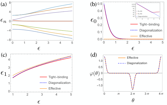
First of all, we expand the Hamiltonian in the eigenstates of $p_{\theta}$. Using particle-hole symmetry, the solutions in the two subspaces $\mathbf{J}_{1}$ and $\mathbf{J}_{2}$, Eq. (16), can be mapped onto each other. Hence, we can focus our discussion on the subset $\mathbf{J}_{1}$ and we take $j_{\max}=48+1/2$ as a reasonable illustration. By numerical matrix diagonalization, we find the full spectrum of the effective edge Hamiltonian. We show the energy of the seven states nearest zero as a function of the scaled Zeeman energy $\epsilon$ in Fig. 2(a) and compare the solution of the effective edge Hamiltonian with a more complete solution using a tight-binding method (see Appendix B for more details) in Figs. 2(b) and (c). In Figs. 2(a) and (b), we can see that a zero mode appears as $\epsilon>2$. By analyzing the results of the diagonalization of the reduced Hamiltonian in the $\mathbf{J}_{1}$ subspace, we find that zero-energy states decay faster than the best exponential fit $\epsilon_{0}\approx 0.528\exp{(-2.66\epsilon)}$, where $\epsilon=0.5E_{Z}k_{F}R/\Delta_{\exp}$. Thus, the energy splitting of zero modes can be suppressed exponentially by increasing the radius $R$ and the Zeeman energy $E_{Z}=\mu_{e}B_{Z}$ (defined in Eq. (II). In Fig. 2(b) and (c), we can see a good agreement between the three methods. We should mention that when $\epsilon$ becomes large the results of the numerical diagonalization and effective methods slightly deviate from the tight-binding model since it contains more states of the 2D bulk. This difference is small in the region of interest and the zero-mode energy is exponentially suppressed to $10^{-6}$ at $\epsilon=3.5$ (see the insert in Fig. 2(b)). As we increase the number of lattice points of the tight-binding calculation, the exponential suppression persists over a larger interval, and thus the flattening of the suppression is due to lattice effects.

We write the $\theta$ representation of the two-component wave function of the zero mode in the $\mathbf{J}_{1}$ subspace defined in Eq. (16), as

The general expansion of $\psi_{0}(\theta)$ is shown in Eq. (119). The zero mode in the other ($\mathbf{J}_{2}$) subspace has wave function $\psi_{0}^{\ast}(\theta)$. Using the symmetry operations in Eqs. (14) and (15), we can prove that

We can thus superimpose the degenerate zero-energy states and express the wave functions of the two Majorana zero modes as

where

We give the full expressions of the wave functions $\psi^{m}_{1}(\theta)$ and $\psi^{m}_{2}(\theta)$, as well as their inter-relations in Appendix C.

We show the angular function $\varphi(\theta)$ calculated through matrix diagonalization for the region $\theta\in[0,4\pi]$ in Fig. 2(d). It is clear from that figure that the Majorana zero mode $\psi^{m}_{1}$ is localized around the point $\theta=0$, and similarly $\psi^{m}_{2}$ is localized around $\theta=\pi$.

After analyzing the numerical results, we would like to get an approximate analytical description for further analysis. Due to the antiperiodic boundary conditions, we cannot approximate the Hamiltonian $h(\theta)$ by linearizing the Dirac mass term around the point it changes sign ($\theta=0$ or $\theta=\pi$) and solve the two independent Dirac-Landau level spectra as in Refs. Park and Recher 2015; Park et al. 2020. The method used in Phong et al. 2017 mixes the two uncoupled sets and thus only describes half the spectrum. To avoid these problems, we will work in the $j$-representation of the edge Hamiltonian but individually solve for a single set, which we take to be $\mathbf{J}_{1}$. To achieve this goal, we first relabel the angular momentum states as

to denote the basis in $\mathbf{J}_{1}$ with integer $k$, and then make the approximation that the low-energy wave functions vary slowly in $k$ so that we can approximately treat $k$ as continuous in this region. Hence, we express the Hamiltonian in terms of $k$ and derivatives with respect to $k$,

Note that $h(\theta)$ defined in Eq. (19) differs from $h(k)$ in the Eq. (III); the latter is a continuous Fourier representation for $h(\theta)$ in the subspace $\mathbf{J}_{1}$ only. To solve most compactly for the eigenstates of $h(k)$, we first apply a unitary transformation $Q^{\dagger}h(k)Q$ to $h(k)$, with

This substantially simplifies the matrix structure of $h(k)$ since it sets the diagonal elements to zero. We then expand the result to the first order in the derivative $\partial_{k}$ to obtain an effective Hamiltonian. The latter can then be simply expressed in terms of harmonic oscillator creation and annihilation operators, $a^{\dagger}$ and $a$ associated with the variable $k$ L.D.Landau and E.M.Lifshitz 1981; Sakurai 1994, as

The spectrum of the effective Hamiltonian is Karzig et al. 2013

This spectrum is the same as that of graphene, treated within the massless-Dirac-fermion approximation, in a uniform magnetic field Girvin and Yang 2019. The eigenstates of $h(k)$ are

where

are the harmonic-oscillator eigenstates. By using the above effective solutions, we can construct the approximate expression of $\varphi(\theta)$, see Appendix C. In Fig. 2(d), we see that the effective expression $\varphi(\theta)$ is extremely close to the matrix diagonalization result. We show more comparisons for different values of $\epsilon>2$ in Fig. 8 in Appendix C.

We now move to study the process of rotating Majorana zero modes on a disk by calculating their dynamical evolution in a uniformly rotating magnetic field. Hence, we focus on the following time-dependent Schrödinger equation

where $H_{\text{edge}}(\theta;\phi(t))$ is defined in Eq. (17), and the angle $\phi(t)$ rotates uniformly with angular velocity $\omega$. In this case, the evolution operator can be exactly solved as follows (for further details, see Appendix D)

Here the parameter $\alpha$ is defined as the ratio of spectral spacing, Eq. (9), the rotation frequency, $\omega_{0}/\omega$, and $h(\theta)$ is defined in Eq. (19). This parameter controls the adiabaticity of the evolution; the larger $\alpha$ is, the more adiabatic the motion becomes, and $\alpha=0$ corresponds to the sudden approximation.

One of the ways to analyze the nature of the motion is the overlap between the final state after a $2\pi$ rotation and the initial state, which we shall assume is one of the zero modes. More specifically, we define the overlap between the final state and the initial zero mode $\psi_{0}$ within the $\mathbf{J}_{1}$ subspace as $\mathcal{A}_{0}=\langle\psi_{0}|\hat{U}^{\alpha}(2\pi)|\psi_{0}\rangle$. If we start from a Majorana zero mode, the overlap between the final state and the initial Majorana zero mode can be related to $\mathcal{A}_{0}$ as

Since $U^{\alpha}(\phi)$ is generated by $p_{\theta}$ and $h(\theta)$ which do not couple the two sets $\mathbf{J}_{1}$ and $\mathbf{J}_{2}$, we limit the calculation to $\mathbf{J}_{1}$. Here we set $\epsilon=5$, $j_{\max}=48+1/2$. We show the resulting overlap $\mathcal{A}_{0}(\alpha)$ in Fig. 3. For small $\alpha$ ($\omega_{0}\ll\omega$), we see that $\text{Re}\{\mathcal{A}_{0}\}$ is very close to 1. This is due to the fact that the system cannot respond quickly enough to the rapid rotation of the magnetic field, so the state has not evolved when the magnetic field comes back to its original value. In the $\alpha>1$ region where $\omega<\omega_{0}$, $\mathcal{A}_{0}$ converges to $-1$ gradually as $\alpha$ increases, which corresponds to the $\pi$ phase shift that always appears for particles with half-integer angular momentum after an adiabatic $2\pi$ rotation. Surprisingly, we can see mild oscillations of $\text{Re}\{\mathcal{A}_{0}\}$ in the $\alpha>1$ region, which reveal non-adiabatic tunneling to excited states. We will discuss this point further in the next section.

Because of the drastic change in behavior of the overlap we observe when moving from the high-frequency region to the low-frequency region, we see that $\alpha=1$, where $\omega=\omega_{0}$, is a potential critical point. To understand this potential phase transition of the overlap $\mathcal{A}_{0}(\alpha)$, we now resort to Floquet analysis for the periodically driven topological superconductor and study the spectrum of the one-cycle evolution operator Barone et al. 1977; Shirley 1965; Bauer et al. 2019. The Floquet Hamiltonian can be defined through the $2\pi$ rotation evolution operator $U^{\alpha}(2\pi)$ as

where the factor $1/2$ represents the minus sign introduced by the left exponential in Eq. (37). We now diagonalize the Floquet Hamiltonian and denote the eigenvalues (quasi-energies) as $\varepsilon_{n}^{\alpha}$.

We calculate the Floquet spectrum through a numerical matrix diagonalization within $\mathbf{J}_{1}$. To study the behavior of the quasi-energies near $\alpha=1$, we show several curves with quasi-energy close to zero for $\alpha$ ranging from $0$ to $1.2$ in Fig. 3(b) and also present the $\alpha$-dependence of $\varepsilon_{0}$ in Fig. 3(c). As we increase $\alpha$ from $0$, we see that the quasi-energy gap closes at $\alpha=1$ and that a new mode appears at fixed quasi-energy $1/2$, and thus phase $\pi$, in the quasi-energy spectrum when $\alpha$ exceeds $1$. From the Floquet perspective, the collapse of the quasi-energy spectrum gives the critical point for the dynamical phase transition related to the evolution of the zero modes. The pi-phase mode in the low-frequency region (large $\alpha$) provides the mechanism by which the zero mode obtains the adiabatic $\pi$ phase shift for a $2\pi$ rotation. The transition point at $\alpha=1$ gives the upper bound of the frequency by which we can preserve the Majorana zero modes under rotation as $\omega_{0}/\hbar=\Delta_{\text{exp}}/(\hbar k_{F}R)$ ($\omega_{0}$ is defined in Eq. (10)).

By application of the angle translation operator $\exp{i\jth\phi}$ to the wave function, which takes its argument $\theta$ to $\theta+\phi$, we have

This equation shows that the Hamiltonian in the co-moving frame is $\omega[h_{F}^{\alpha}(\theta)-\frac{1}{2}]$. Thus, the Floquet pi-mode of $h_{F}$ is the zero mode of this Hamiltonian. For small $\omega$, the solutions to the domain-wall model contain soliton states made up of two counter-propagating chiral states, with the soliton located at the points where the Dirac mass term changes sign. However, when $\omega$ exceeds $\omega_{0}$, both left-hand and right-hand chiral states all propagate in the same direction, and the domain-wall bound state disappears. In fact, a similar dynamic model has been used to describe moving domain wall solitons in an infinite line Jackiw and Rebbi 1976; Karzig et al. 2013; Conlon et al. 2019. In Ref. Karzig et al. 2013, the authors studied the exact spectrum of the boosted model through a global Lorentz transformation in a the flat metric. Unfortunately, the same global transformation fails in our reduced 1D model with circular geometry. Thus, we resort to a Floquet analysis. Note that our analysis can be applied not only to intercalated Bi₂Se₃ but also to generic Dirac-type models in a disc geometry.

In this section, we use second-order perturbation theory Mostafazadeh 1997; Frasca 1998 to interpret the frequency-dependence of the oscillations of $\mathcal{A}_{0}$ in the low-frequency (large $\alpha$) regime and show that they can be related to non-adiabatic tunneling in the co-rotating frame.

To approach this problem, we work in the $k$-representation as set out in Eqs. (III-37) and work in a co-moving reference frame, Eq. (42). As before, we simplify the algebra by transforming the evolution operator by the operator $Q$, Eq. (III) so that the result can be expressed in terms of harmonic oscillator creation and annihilation operators. Using time-dependent perturbation theory, we expand the transformed evolution operator to the second order in $1/\alpha$ and find

where

Operating with the above effective evolution operator on the initial zero mode $\psi_{0}$, we have:

In the above equations, $\epsilon_{1}=\sqrt{4\epsilon}$ is the energy gap between the zero mode and the lowest positive energy state. Since the transition probabilities obey $|a_{0}(\phi)|^{2}\approx 1-(|a_{1}(\phi)|^{2}+|a_{-1}(\phi)|^{2})$, the non-adiabatic tunneling in the low-frequency regime mostly happens between $\psi_{0}$, and $\psi_{\pm 1}$ as defined in Eq. (34). Using the result Eq. (45), we can obtain an effective expression of the overlap $\mathcal{A}_{0}$ for a full one-cycle rotation,

This equation accurately describes the behavior of the frequency-dependent oscillation in the overlap $\mathcal{A}_{0}(\alpha)$. The minus sign originates from the anti-periodic boundary conditions on the wave function. We compare the results of a matrix diagonalization and the effective theory in Fig. 4. We can see that the result obtained with the two methods are very close. In the inset of Fig. 4, we show the highest and lowest points of the curve $\mathcal{A}_{0}$. The deviation between exact-diagonalization and effective results in Fig. 4 is about $0.1\%$.

From Eq. (48), we can see that the non-adiabatic error can be almost zero when the rotation period of the magnetic field is an integer multiple of the frequency-independent period $2\pi/(\sqrt{4\epsilon}\omega_{0})$.

This result can be understood as follows. In the co-rotating frame, the time-dependent evolution is governed by Eq. (42). The term $-p_{\theta}$ in $h_{F}$ can make the initial zero mode tunnel to other eigenstates of the equilibrium Hamiltonian. Also, the transition amplitude between the initial zero mode and the final state is equal to $1-\omega^{2}\sin{^2}\left(\sqrt{4\epsilon}\omega_{0}t/2\right)/(2\omega_{0}^{2})$, and vanishes when the $t$ is an integer multiple of the tunneling period, i.e., in the perturbative and adiabatic regime (in the case with $\epsilon=5$, the region starts at about $\alpha>4$), at frequencies

with $\nu$ an integer, the final state after one full rotation of the magnetic field has overlap $-1$ with the initial state. For a $2\pi$ rotation ($\Delta\phi=2\pi$), the integer $\nu$ should be larger than $18$ within the regime $\alpha>4$. Since $\nu$ is large, the difference of the two nearest-neighbor high-fidelity frequencies can be approximated as $\omega_{\nu}(2\pi)-\omega_{\nu+1}(2\pi)\approx\sqrt{4\epsilon}\omega_{0}/\nu^{2}$.

In order to see how realistic our theoretical approach is, we need to estimate the parameters of the model: From Refs. Phong et al. 2017; Zhang et al. 2009b; Hor et al. 2010; Sasaki et al. 2011; Wray et al. 2011; Sandilands et al. 2014, we estimate $\Delta_{\exp}=0.6\text{meV}$, $k_{F}=0.1\,\text{\AA}^{-1}$. For a device size $R=10\mu\text{m}$, we determine the dimensionless parameters as $\lambda=10^{4}$, $\gamma=\Delta_{\exp}^{2}/(2\bar{\epsilon}_{F}^{2})=4.5\times 10^{-6}$, and $\omega_{c}=\omega_{0}/\hbar\approx 91.2\,\text{MHz}$. To obtain a zero mode, one needs $\epsilon>2$, which in turn implies that the in-plane magnetic field should be larger than $B_{0}=4\omega_{0}/\mu_{e}\approx 4\,\text{mT}$. For $\epsilon=5$ as used in the main text, the corresponding magnetic field is about $10\,\text{mT}$. In this case, when the rotation frequency exceeds $\omega_{c}=91.2\,\text{MHz}$, Majorana pi-modes appear and the region where we can perform quasi-adiabatic 2$\pi$ rotations is $\alpha>4$, corresponding to $\omega<\omega_{c}/4\approx 22.8\,\text{MHz}$. Since the difference between the two nearest-neighbor high-fidelity frequencies is about $407/\nu^{2}$MHz and $\nu$ is larger than 18, we require the frequency width of the rotating magnetic field smaller than $0.315$MHz.

In conclusion, we have made progress on two issues: Firstly, we show through a rigorous process how to reduce a 2D Hamiltonian of a second-order $p$-wave superconductor with disc geometry to a 1D Hamiltonian for edge space and build an effective model to give the approximated analytical solution, which improves on the results in Ref. Phong et al. 2017, and also allows us to study the evolution in detail; Secondly, we show that the separation between diabatic and adiabatic motion of rotating Majorana zero-modes in the system exhibits an interesting dynamical phase transition at $\alpha=1$. Beyond this transition point, we have been able to give a detailed numerical and analytical analysis of the approach to adiabaticity. Thus the effective matrix model studied here, with its simple solution, could be of further interest.

We show that at a set of regularly spaced rotation frequencies, we have substantially higher fidelity; by choosing to work at one of these optimal frequencies, one can dramatically reduce quasi-particle poisoning and increase the robustness of the translation of the Majorana states, and thus the manipulation of quantum information in such a device. Our analysis ignores other sources of errors, such as those caused by disorders or fluctuations in the magnetic field, etc. These will be the subject of future work.

References

- Nayak et al. (2008) C. Nayak, S. H. Simon, A. Stern, M. Freedman, and S. Das Sarma, Non-abelian anyons and topological quantum computation, Rev. Mod. Phys. 80, 1083 (2008).
- O’Brien et al. (2018) T. E. O’Brien, P. Rożek, and A. R. Akhmerov, Majorana-based fermionic quantum computation, Phys. Rev. Lett. 120, 220504 (2018).
- Kitaev (2001) A. Y. Kitaev, Unpaired majorana fermions in quantum wires, Physics-Uspekhi 44, 131 (2001).
- Ivanov (2001) D. A. Ivanov, Non-abelian statistics of half-quantum vortices in -wave superconductors, Phys. Rev. Lett. 86, 268 (2001).
- Aasen et al. (2016) D. Aasen, M. Hell, R. V. Mishmash, A. Higginbotham, J. Danon, M. Leijnse, T. S. Jespersen, J. A. Folk, C. M. Marcus, K. Flensberg, and J. Alicea, Milestones toward majorana-based quantum computing, Phys. Rev. X 6, 031016 (2016).
- Qi et al. (2009) X.-L. Qi, T. L. Hughes, S. Raghu, and S.-C. Zhang, Time-reversal-invariant topological superconductors and superfluids in two and three dimensions, Phys. Rev. Lett. 102 (2009).
- Zhang et al. (2009a) H. Zhang, C.-X. Liu, X.-L. Qi, X. Dai, Z. Fang, and S.-C. Zhang, Topological insulators in bi2se3, bi2te3 and sb2te3 with a single dirac cone on the surface, Nature Physics 5, 438 (2009a).
- Fu and Berg (2010) L. Fu and E. Berg, Odd-parity topological superconductors: Theory and application to , Phys. Rev. Lett. 105, 097001 (2010).
- Liu et al. (2010) C.-X. Liu, X.-L. Qi, H. Zhang, X. Dai, Z. Fang, and S.-C. Zhang, Model hamiltonian for topological insulators, Phys. Rev. B 82, 045122 (2010).
- Hsieh and Fu (2012) T. H. Hsieh and L. Fu, Majorana fermions and exotic surface andreev bound states in topological superconductors: Application to , Phys. Rev. Lett. 108, 107005 (2012).
- Venderbos et al. (2016) J. W. F. Venderbos, V. Kozii, and L. Fu, Odd-parity superconductors with two-component order parameters: Nematic and chiral, full gap, and majorana node, Phys. Rev. B 94, 180504 (2016).
- Phong et al. (2017) V. T. Phong, N. R. Walet, and F. Guinea, Majorana zero modes in a two-dimensional -wave superconductor, Phys. Rev. B 96, 060505 (2017).
- Chirolli et al. (2017) L. Chirolli, F. de Juan, and F. Guinea, Time-reversal and rotation symmetry breaking superconductivity in dirac materials, Phys. Rev. B 95, 201110 (2017).
- Hor et al. (2010) Y. S. Hor, A. J. Williams, J. G. Checkelsky, P. Roushan, J. Seo, Q. Xu, H. W. Zandbergen, A. Yazdani, N. P. Ong, and R. J. Cava, Superconductivity in and its implications for pairing in the undoped topological insulator, Phys. Rev. Lett. 104, 057001 (2010).
- Sasaki et al. (2011) S. Sasaki, M. Kriener, K. Segawa, K. Yada, Y. Tanaka, M. Sato, and Y. Ando, Topological superconductivity in , Phys. Rev. Lett. 107, 217001 (2011).
- Schindler et al. (2018) F. Schindler, A. M. Cook, M. G. Vergniory, Z. Wang, S. S. P. Parkin, B. A. Bernevig, and T. Neupert, Higher-order topological insulators, Science Advances 4 (2018).
- Zhu (2018) X. Zhu, Tunable majorana corner states in a two-dimensional second-order topological superconductor induced by magnetic fields, Phys. Rev. B 97, 205134 (2018).
- Yan (2019) Z. Yan, Higher-order topological odd-parity superconductors, Phys. Rev. Lett. 123, 177001 (2019).
- Zhang et al. (2013) F. Zhang, C. L. Kane, and E. J. Mele, Time-reversal-invariant topological superconductivity and majorana kramers pairs, Phys. Rev. Lett. 111, 056402 (2013).
- Yan et al. (2018) Z. Yan, F. Song, and Z. Wang, Majorana corner modes in a high-temperature platform, Phys. Rev. Lett. 121, 096803 (2018).
- Wang et al. (2018) Q. Wang, C.-C. Liu, Y.-M. Lu, and F. Zhang, High-temperature majorana corner states, Phys. Rev. Lett. 121, 186801 (2018).
- Wu et al. (2020) Y.-J. Wu, J. Hou, Y.-M. Li, X.-W. Luo, X. Shi, and C. Zhang, In-plane zeeman-field-induced majorana corner and hinge modes in an -wave superconductor heterostructure, Phys. Rev. Lett. 124, 227001 (2020).
- Park and Recher (2015) S. Park and P. Recher, Detecting the exchange phase of majorana bound states in a corbino geometry topological josephson junction, Phys. Rev. Lett. 115, 246403 (2015).
- Park et al. (2020) S. Park, H.-S. Sim, and P. Recher, Electron-tunneling-assisted non-abelian braiding of rotating majorana bound states, Phys. Rev. Lett. 125, 187702 (2020).
- Zhang et al. (2020a) S.-B. Zhang, A. Calzona, and B. Trauzettel, All-electrically tunable networks of majorana bound states, Phys. Rev. B 102, 100503 (2020a).
- Zhang et al. (2020b) S.-B. Zhang, W. B. Rui, A. Calzona, S.-J. Choi, A. P. Schnyder, and B. Trauzettel, Topological and holonomic quantum computation based on second-order topological superconductors, Phys. Rev. Research 2, 043025 (2020b).
- Cheng et al. (2011) M. Cheng, V. Galitski, and S. Das Sarma, Nonadiabatic effects in the braiding of non-abelian anyons in topological superconductors, Phys. Rev. B 84, 104529 (2011).
- Scheurer and Shnirman (2013) M. S. Scheurer and A. Shnirman, Nonadiabatic processes in majorana qubit systems, Phys. Rev. B 88, 064515 (2013).
- Karzig et al. (2013) T. Karzig, G. Refael, and F. von Oppen, Boosting majorana zero modes, Phys. Rev. X 3, 041017 (2013).
- Amorim et al. (2015) C. S. Amorim, K. Ebihara, A. Yamakage, Y. Tanaka, and M. Sato, Majorana braiding dynamics in nanowires, Phys. Rev. B 91, 174305 (2015).
- Karzig et al. (2015) T. Karzig, A. Rahmani, F. von Oppen, and G. Refael, Optimal control of majorana zero modes, Phys. Rev. B 91, 201404 (2015).
- Conlon et al. (2019) A. Conlon, D. Pellegrino, J. K. Slingerland, S. Dooley, and G. Kells, Error generation and propagation in majorana-based topological qubits, Phys. Rev. B 100, 134307 (2019).
- Shirley (1965) J. H. Shirley, Solution of the schrödinger equation with a hamiltonian periodic in time, Phys. Rev. 138, B979 (1965).
- Barone et al. (1977) S. R. Barone, M. A. Narcowich, and F. J. Narcowich, Floquet theory and applications, Phys. Rev. A 15, 1109 (1977).
- Thouless et al. (1982) D. J. Thouless, M. Kohmoto, M. P. Nightingale, and M. den Nijs, Quantized hall conductance in a two-dimensional periodic potential, Phys. Rev. Lett. 49, 405 (1982).
- Stone and Roy (2004) M. Stone and R. Roy, Edge modes, edge currents, and gauge invariance in superfluids and superconductors, Phys. Rev. B 69, 184511 (2004).
- Read and Green (2000) N. Read and D. Green, Paired states of fermions in two dimensions with breaking of parity and time-reversal symmetries and the fractional quantum hall effect, Phys. Rev. B 61, 10267 (2000).
- Sato and Ando (2017) M. Sato and Y. Ando, Topological superconductors: a review, Reports on Progress in Physics 80, 076501 (2017).
- Bernevig and Hughes (2013) B. A. Bernevig and T. L. Hughes, Topological Insulators and Topological Superconductors (Princeton University Press, 2013).
- Michaeli and Fu (2012) K. Michaeli and L. Fu, Spin-orbit locking as a protection mechanism of the odd-parity superconducting state against disorder, Phys. Rev. Lett. 109, 187003 (2012).
- Clogston (1962) A. M. Clogston, Upper limit for the critical field in hard superconductors, Phys. Rev. Lett. 9, 266 (1962).
- Jackiw and Rebbi (1976) R. Jackiw and C. Rebbi, Solitons with fermion number 1/2, Phys. Rev. D 13, 3398 (1976).
- Su et al. (1979) W. P. Su, J. R. Schrieffer, and A. J. Heeger, Solitons in polyacetylene, Phys. Rev. Lett. 42, 1698 (1979).
- L.D.Landau and E.M.Lifshitz (1981) L.D.Landau and E.M.Lifshitz, Quantum Mechanics, 3rd ed. (Butterworth-Heinemann, 1981).
- Sakurai (1994) J. J. Sakurai, Modern quantum mechanics, rev. ed ed. (Addison-Wesley Pub. Co, 1994).
- Girvin and Yang (2019) S. M. Girvin and K. Yang, Modern Condensed Matter Physics (Cambridge University Press, 2019).
- Bauer et al. (2019) B. Bauer, T. Pereg-Barnea, T. Karzig, M.-T. Rieder, G. Refael, E. Berg, and Y. Oreg, Topologically protected braiding in a single wire using floquet majorana modes, Phys. Rev. B 100, 041102 (2019).
- Mostafazadeh (1997) A. Mostafazadeh, Quantum adiabatic approximation and the geometric phase, Phys. Rev. A 55, 1653 (1997).
- Frasca (1998) M. Frasca, Duality in perturbation theory and the quantum adiabatic approximation, Phys. Rev. A 58, 3439 (1998).
- Zhang et al. (2009b) G. Zhang, H. Qin, J. Teng, J. Guo, Q. Guo, X. Dai, Z. Fang, and K. Wu, Quintuple-layer epitaxy of thin films of topological insulator bi2se3, Applied Physics Letters 95, 053114 (2009b).
- Wray et al. (2011) L. A. Wray, S. Xu, Y. Xia, D. Qian, A. V. Fedorov, H. Lin, A. Bansil, L. Fu, Y. S. Hor, R. J. Cava, and M. Z. Hasan, Spin-orbital ground states of superconducting doped topological insulators: A majorana platform, Phys. Rev. B 83, 224516 (2011).
- Sandilands et al. (2014) L. J. Sandilands, A. A. Reijnders, M. Kriener, K. Segawa, S. Sasaki, Y. Ando, and K. S. Burch, Doping-dependent charge dynamics in , Phys. Rev. B 90, 094503 (2014).
- Arfken and Weber (1999) G. B. Arfken and H. J. Weber, Mathematical Methods for Physicists (AAPT, 1999).
- Bellman (1961) Bellman, A brief introduction to theta functions (International Thomson Publishing, 1961).