Chapter Ground and Applied-Field-Driven Magnetic States of Antiferromagnets

Hai-Feng Li Thanks: E-mail address: haifengli@um.edu.mo Affiliation: Joint Key Laboratory of the Ministry of Education,Institute of Applied Physics and Materials Engineering,University of Macau, Macao, China Zikang Tang Thanks: E-mail address: zktang@um.edu.mo Affiliation: Joint Key Laboratory of the Ministry of Education,Institute of Applied Physics and Materials Engineering,University of Macau, Macao, China

Abstract

As discussed in this chapter, we develop a mean-field mathematical method to calculate the ground states of antiferromagnets and better understand the applied magnetic-field induced exotic properties. Within antiferromagnetic materials competitive and cooperative interactions exist leading to substance extraordinary magnetic states. Our calculations predict that applying a magnetic field to antiferromagnets can switch it from one magnetic state to another. These include antiferromagnetic ground state, spin-flop transition, spin-flopped state, spin-flip transition and spin-flipped state. Our framework successfully demonstrates these phase changes. With this, a map of all equilibrium magnetic ground states, as well as the respective equilibrium phase conditions, are derived. Our study provides insight into the origins of the various magnetic states.

Keywords: antiferromagnet, ground state, magnetic-field effect, spin flop, spin flip

1. Introduction

Strongly-correlated electron materials are given that name due to the fact that a huge amount of electrons within them interact with each other to give the substance nontrivial properties such as the high $T_{\textrm{c}}$ superconductivity [1, 2, 3, 4, 5, 6], multiferroicity [7, 8, 9, 10, 11, 12, 13, 14], colossal magnetoresistance effect [15, 16, 17, 18, 19, 20], metal-insulator transition [21, 22, 23, 24, 25, 26, 27], or giant magnetostriction effect [17, 19, 28]. Most of these extraordinary macroscopic functionalities are causally linked with magnetism. For example, the unconventional superconductivity appears normally in materials where the long-range antiferromagnetic (AFM) states are partially or completely suppressed upon hole- or electron-doping, or by pressure. Magnetism is thus connected with the unconventional superconductivity [29, 30, 31, 32, 33, 34, 35, 36, 37, 38, 39, 40, 41, 42, 43, 44, 45, 46, 47, 48, 49, 50, 51, 52, 53, 54, 55, 56, 57, 58]. A full and consistent understanding of these interesting experimental observations has yet to be achieved [59, 60, 61, 62, 63, 64, 65, 66, 67, 68, 69, 70, 71, 72, 73, 74, 75, 76, 77, 78, 79, 80, 81, 82] and necessitates a complete reveal of all possible magnetic ground states, and especially magnetic-field driven phase transitions and fluctuations of magnets. This is the central topic of this chapter.

Materials consist of atoms. They don’t behave as completely free ions in a crystal. On the contrary, they all interact with each other or their surroundings. Such interactions are sometimes large and significant and cannot be overlooked, especially for magnetic ions. Magnetic interactions such as the dipolar, direct exchange, superexchange, double exchange, anisotropic exchange, or the Ruderman-Kittel-Kasuya-Yosida exchange interaction play an important role in bridging the communications between spin moments in a crystal—thereby leading to potential long-range ordered magnetic states like ferromagnetism or antiferromagnetism.

All spin moments within a ferromagnet, as schematically shown in Figure 1(a), are in parallel alignment, producing a spontaneous magnetization even in the absence of an applied field. While in an AFM state, they lie in antiparallel alignment for adjacent spin moments (Figure 1(b)). The spin arrangements in an antiferromagnet can be decomposed into two ferromagnetic (FM)-like interpenetrating states as shown in Figures 1(b1) and 1(b2), where two orientations of the spin moments in sublattices are completely opposite. The strong coupling of spin, charge, orbital and lattice degrees of freedom leads to various long-range spin ordered states [83, 84, 85, 86]. Some of the frequent AFM ground states are schematically illustrated in Figure 2. These magnetic states are strongly dependent on the chemical pressure and temperature [87, 88]. For example, at room temperature, Nd_1-xSr_xMnO₃ [83] shows the FM state for 0.3 $<$ x $<$ 0.5. When doped further, the compounds show the A-type AFM state for 0.5 $<$ x $<$ 0.7. When the doping level is above 0.7, the C-type AFM state appears [89, 90]. Above 77 K, YVO₃ shows the C-type AFM spin order, followed by a transition to the G-type AFM state below 77 K [91].

For the traditional spin-flop (SFO) transition, typically a first-order (FO) type in character, and limited to a collinear antiferromagnet below the Néel transition temperature, the AFM sublattice spins suddenly rotate 90^∘ so that they are perpendicular to the original AFM easy axis while applying a magnetic field (B) along the AFM easy axis, and when the applied magnetic-field reaches a critical value $(B_{\textrm{SFO}})$ . For the so-called spin-flip (SFI) transition [92, 93], as the field strength further increases $(B>B_{\textrm{SFO}})$ , the flopped spins gradually tilt toward the field direction until they are completely aligned at a sufficiently high magnetic field $(B_{\textrm{SFI}})$ . These magnetic-field driven phase transitions are schematically shown in Figure 3.

It is hard to experimentally identify the nature of a SFO transition (FO or second-order (SO) type) because of the technically unavoidable effect of misalignment between the relevant AFM easy axis and an applied-field direction. In 1936, Néel [94] theoretically proposed the possibility for a SFO transition. It was then experimentally observed in a CuCl₂ $\cdot$ 2H₂O single crystal [95]. After that, the SFO phase transition has been extensively investigated, and the phenomenological theory has also been comprehensively developed [96, 97, 98, 99, 100, 101, 102, 103, 104, 105, 106, 107, 108, 109, 110, 111, 112, 113, 114, 115, 116, 117, 118, 119, 120, 121, 122]. It is generally confirmed that the SFO phase transition is of FO type [85, 123, 124, 125, 126, 127, 128, 129, 130, 131, 132, 133, 134, 135, 136, 137]. On the contrary, some observed SFO transitions [130, 138, 139] don’t show a magnetic hysteresis effect that is the characteristic feature of a FO phase transition. The broad SFO phase transition was attributed to a low magnetic anisotropy [130, 139], a softening of surface magnons [140], a domain effect, or a misalignment of applied magnetic field with regard to the AFM easy axis [128, 141, 142]. It is pointed out that such types of continuous magnetic phase transitions [143, 144], the absence of magnetic hysteresis, and the experimental observation of a possible intermediate phase in the SFO compound CoBr₂ $\cdot$ 6[0.48D₂O, 0.52H₂O] [145, 146], cast considerable doubt on the nature of SFO transitions. Actually, it may indicate a SO type phase transition. It is hard to distinguish experimentally the origin of the SO-type-like SFO transition [128, 141, 142] since the allowed small misalignment for a FO SFO transition is usually beyond the present experimental accuracy, and any larger misalignment may change a FO-type into a SO-type broadening SFO transition. Early theoretical calculations predicted an intermediate regime bordering with the AFM and spin-flopped states [147, 148, 149]. These predications have not yet been confirmed based on the principle of minimum total potential free energy, and most of the theoretical models overlooked the singe-ion anisotropy. This is extremely important in the case of lanthanides and actinides [150, 151, 152, 153, 154, 155]. Additionally, a rotating FM phase was also predicted for a SFO antiferromagnet [147, 156]. However, this kind of unusual magnetic phase has never been observed experimentally, which renders the validity of the phase undecided [93].

Here a mathematical method for a better understanding of the exotic properties of magnetic materials was proposed. We have developed calculations that predict the magnetic-field driven SFO and SFI phase transitions of localized collinear antiferromagnets. Our model unifies all possible magnetic ground and excited states and reveals some interesting magnetic phase transitions and coexistences of some of the magnetic states. This study unambiguously reveals a SO-type SFO transition. We conclusively rule out the possibility for a rotating FM-like magnetic state [147]. This model calculation consistently covers all possible magnetic-field driven magnetic states of collinear antiferromagnets, which sheds light on the origins of the various magnetic states. We further deduce an alternative to the estimation of magnetic exchange parameters [93].

2. Materials and Methods

We limit our calculation to purely-localized collinear AFM systems and overlook the effect of valence electrons on magnetic couplings. In this case, for two-sublattice AFM spins (Figure 3), the Hamiltonian terms consist of four parts: magnetic exchange, spin-exchange anisotropy, single-ion anisotropy and Zeeman coupling to an external magnetic field. We assume that both AFM easy direction $M^{0}_{-}M^{0}_{+}$ and localized sublattice moments $M_{+}$ and $M_{-}$ are along the z axis (Figure 3(a)), and the subsequent completely-flopped spins are parallel to the x axis (Figures 3(c)), thus, the sublattice-moment vectors within the xz plane (Figure 3(b)) can be written as [93]:

\displaystyle\left\{\begin{array}[]{ll}\begin{split}\widehat{M}_{+}&=M_{+}[\hat{x}sin(\phi{-}\beta_{1}){+}\hat{z}cos(\phi{-}\beta_{1})]{\color[rgb]{1,1,1},}{\color[rgb]{1,1,1}a}\textrm{and}\\ \widehat{M}_{-}&={-}M_{-}[\hat{x}sin(\phi{+}\beta_{2}){+}\hat{z}cos(\phi{+}\beta_{2})],\end{split}\end{array}\right.

respectively, where $\hat{x}$ and $\hat{z}$ are the unit vectors along the $x$ and $z$ axes, respectively. The angles $\phi$ , $\beta_{1}$ and $\beta_{2}$ are defined in Figure 3. Therefore, the sublattice-moment related free energy (E) within a mean-field approximation can be calculated by [93]:

\displaystyle\begin{split}\emph{E}=&{\color[rgb]{1,1,1}1}\emph{J}\emph{M}_{+}{\cdot}\emph{M}_{-}{+}\gamma\emph{M}_{+}^{z}\emph{M}_{-}^{z}{-}D[(\emph{M}_{+}^{z})^{2}{+}(\emph{M}_{-}^{z})^{2}]{-}B(\emph{M}_{+}^{z}{+}\emph{M}_{-}^{z})\\ =&{-}\emph{J}M_{+}M_{-}\cos(\beta_{1}{+}\beta_{2}){-}\gamma M_{+}M_{-}\cos(\phi{-}\beta_{1})\cos(\phi{+}\beta_{2})\\ &{-}D[M^{2}_{+}\cos^{2}(\phi{-}\beta_{1}){+}M^{2}_{-}\cos^{2}(\phi{+}\beta_{2})]\\ &{-}B[M_{+}\cos(\phi{-}\beta_{1}){-}M_{-}\cos(\phi{+}\beta_{2})],\end{split}

(3)

where the four terms in turn represent the four Hamiltonian components, and J $(>0)$ , $\gamma$ and D are the AFM coupling, anisotropic exchange and single-ion anisotropic energies, respectively. In an unsaturation magnetic state, with increasing magnetic field B $(\parallel z$ axis) as shown in Figures 3(a) and 3(b), the sublattice moment $M_{+}$ ( $M_{-}$ ) increases (decreases) as a consequence, which leads to $\beta_{1}<\beta_{2}$ . At the lowest temperature T = 0 K, i.e., in a real saturation magnetic state, $M_{+}\equiv M_{-}=M_{0}$ , and thus $\beta_{1}\equiv\beta_{2}=\beta$ . Hence, equation (3) can be simplified as [93]:

\displaystyle\begin{split}\emph{E}=&{-}\emph{J}M_{0}^{2}\cos(2\beta){-}\gamma M_{0}^{2}\cos(\phi{-}\beta)\cos(\phi{+}\beta){-}DM_{0}^{2}[\cos^{2}(\phi{-}\beta)\\ &{+}\cos^{2}(\phi{+}\beta)]{-}BM_{0}[\cos(\phi{-}\beta){-}\cos(\phi{+}\beta)]\\ =&{-}\emph{J}M_{0}^{2}\cos(2\beta){-}\frac{\gamma M_{0}^{2}}{2}[\cos(2\phi){+}\cos(2\beta)]{-}DM_{0}^{2}[1\\ &{+}\cos(2\phi)\cos(2\beta)]{-}2BM_{0}\sin\phi\sin\beta.\end{split}

(4)

3. Results

3.1. Equilibrium Magnetic State

Possible magnetic ground and excited states can be derived from different combinations of the FO partial differential equations, i.e., $\frac{\partial E}{\partial\beta}=\frac{\partial E}{\partial\phi}=$ 0 with equation (4) [93]:

	$\displaystyle\left.\begin{array}[]{r r}2DM_{0}\sin\phi\cos(2\beta)+\gamma M_{0}\sin\phi-B\sin\beta=0\\ 2JM_{0}\sin\beta+2DM_{0}\cos(2\phi)\sin\beta+\gamma M_{0}\sin\beta-B\sin\phi=0\end{array}\right\};$
	$\displaystyle\left.\begin{array}[]{r r}\cos\phi=0\\ 2JM_{0}\sin\beta+2DM_{0}\cos(2\phi)\sin\beta+\gamma M_{0}\sin\beta-B\sin\phi=0\end{array}\right\};$
	$\displaystyle\left.\begin{array}[]{r r}2DM_{0}\sin\phi\cos(2\beta)+\gamma M_{0}\sin\phi-B\sin\beta=0\\ \cos\beta=0\end{array}\right\};$
	$\displaystyle\left.\begin{array}[]{r r}\cos\phi=0\\ \cos\beta=0\end{array}\right\}.$

We solved the four combinations (3.1.-3.1.) and correlated the results with physical meanings accordingly [93].

(i) From the combination (3.1.), we obtained two solutions:

\displaystyle\left.\begin{array}[]{r r}\textrm{(A)}\sin\phi=\sin\beta=0,i.e.,\phi=\beta=0;\\ \\ \textrm{(B)}\sin\phi=\delta\sin\beta,\textrm{where }\sin\beta=\sqrt{\frac{\delta M_{0}(2D{+}\gamma){-}B}{4\delta M_{0}D}}{\color[rgb]{1,1,1},}\\ \\ \textrm{and }\delta=\sqrt{\frac{2J{+}2D{+}\gamma}{2D{+}\gamma}}.\\ \end{array}\right\}

Here the case (A) is related to an AFM ground state (Figure 3(a)). The case (B) indicates a correlated change of $\phi$ with $\beta$ . In Figure 3, $0^{\circ}\leq\phi\leq 90^{\circ}$ . As a result, there exist two boundary magnetic fields that correspond to the second solution of the combination (3.1.). When $\phi=0$ , $\sin\phi=\delta\sin\beta=0$ . One can thus deduce that the initial magnetic field for the beginning of the SFO transition

\displaystyle B_{\textrm{SFOB}}=M_{0}\sqrt{(2D{+}\gamma)(2J{+}2D{+}\gamma)}.

(23)

When $\phi=\frac{\pi}{2}$ , $\delta\sin\beta=1$ , the final magnetic field for the ending of the SFO transition

\displaystyle B_{\textrm{SFOF}}=M_{0}(2J{-}2D{+}\gamma)\sqrt{\frac{2D{+}\gamma}{2J{+}2D{+}\gamma}}.

(24)

When $B_{\textrm{SFOB}}\geq B_{\textrm{SFOF}}$ , we can derive the precondition of a FO SFO transition: $D\geq 0$ and $2D{+}\gamma>0$ . Further, when $B_{\textrm{SFOB}}<B_{\textrm{SFOF}}$ , i.e., ${-}\frac{1}{2}\gamma<D<0$ , a SO SFO transition surprisingly occurs spontaneously. This originates from a negative single-ion anisotropy that is additionally restricted to a certain range by the anisotropic exchange interaction ( $\gamma$ ).

(ii) The combination (3.1.) implies that

\displaystyle\phi

\displaystyle=

\displaystyle\frac{\pi}{2},\textrm{and }\sin\beta=\frac{B}{M_{0}(2J{-}2D{+}\gamma)},

(25)

which corresponds to the process of a SFI transition (Figure 3(d)). When

\displaystyle B=B_{\textrm{SFI}}=M_{0}(2J{-}2D{+}\gamma),

(26)

$\beta=\frac{\pi}{2}$ , implying a spin-flipped (SFID) state (Figure 3(e)). Therefore, the SFI transition field $B_{\textrm{SFI}}$ depends not only on the moment size $M_{0}$ but also on the values of $J$ , $\gamma$ and $D$ .

(iii) From the combination (3.1.), we can deduce that

\displaystyle\beta

\displaystyle=

\displaystyle\frac{\pi}{2},\textrm{and }\sin\phi=\frac{B}{M_{0}(\gamma{-}2D)}.

(27)

When $\beta=\frac{\pi}{2}$ , both sublattice moments $M_{+}$ and $M_{-}$ are perpendicular to the AFM axis $M^{0}_{-}M^{0}_{+}$ , forming a rotating FM-like state. The value of $\phi$ can intrinsically be modified by a change in magnetic field $B$ .

(iv) The combination (3.1.) indicates $\phi=\beta=\frac{\pi}{2}$ . This corresponds to a SFID state (Figure 3(e)).

3.2. Free Energy Calculation

In the following, we calculated free-energy scales of the derived magnetic states by substituting their respective equilibrium phase conditions back into equation (4). We thus obtain [93]:

\displaystyle\left\{\begin{split}E_{\textrm{AFM}(z{-}\textrm{axis})}=\text{{\color[rgb]{1,1,1}a}}&{-}(J{+}\gamma{+}2D)M_{0}^{2}\text{{\color[rgb]{1,1,1}aa}}\qquad\qquad(0\leq B<B_{\textrm{SFO}});\\ E_{x{-}\textrm{axis}}=\text{{\color[rgb]{1,1,1}a}}&{-}JM_{0}^{2}\text{{\color[rgb]{1,1,1}1}}\qquad\qquad\qquad\qquad(\phi=90^{\circ},\beta=0^{\circ});\\ E_{\textrm{SFI}}=\text{{\color[rgb]{1,1,1}a}}&{-}JM_{0}^{2}{-}\frac{B^{2}}{2J{-}2D{+}\gamma}\qquad(B_{\textrm{SFO}}\leq B<B_{\textrm{SFI}});\\ E_{\textrm{SFID}}=\text{{\color[rgb]{1,1,1}a}}&[{-}J{-}(2J{-}2D{+}\gamma)]M_{0}^{2}\text{{\color[rgb]{1,1,1}a}}\qquad\qquad(B=B_{\textrm{SFI}});\\ E_{\textrm{FM{-}like}}=\text{{\color[rgb]{1,1,1}a}}&JM_{0}^{2}{-}\frac{B^{2}}{\gamma{-}2D}\qquad\qquad[0\leq B\leq M_{0}(\gamma{-}2D)];\end{split}\right.

(28)

in addition, the one corresponding to the SO SFO transition is:

\displaystyle\left\{\begin{split}E_{\textrm{SO{-}SFO}}=\text{{\color[rgb]{1,1,1}a}}&{-}JM_{0}^{2}(1{-}2\sin^{2}\beta){-}\gamma M^{2}_{0}(1{-}\sin^{2}\beta{-}\delta^{2}\sin^{2}\beta)\\ \text{{\color[rgb]{1,1,1}a}}&{-}DM^{2}_{0}[1{+}(1{-}2\delta^{2}\sin^{2}\beta)(1{-}2\sin^{2}\beta)]{-}2BM_{0}\delta\sin^{2}\beta\\ \\ &\text{{\color[rgb]{1,1,1}a}}(\sin\beta=\sqrt{\frac{\delta M_{0}(2D{+}\gamma){-}B}{4\delta M_{0}D}},\delta=\sqrt{\frac{2J{+}2D{+}\gamma}{2D{+}\gamma}};\\ &\qquad\qquad\text{{\color[rgb]{1,1,1}aa}}{-}\frac{1}{2}\gamma<D<0;B_{\textrm{SFOB}}\leq B<B_{\textrm{SFOF}}).\end{split}\right.

(29)

We quantitatively compared the free energies.

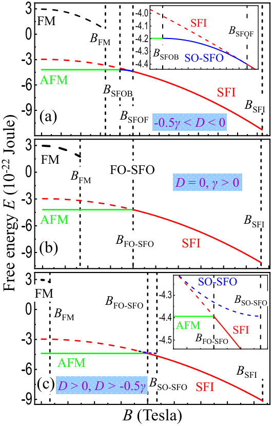
(i) The case of the SO SFO transition ( ${-}\frac{1}{2}\gamma<D<0$ ). Supposing that $M_{\textrm{0}}$ = 4 $\mu_{\textrm{B}}$ , J = 2 T/ $\mu_{\textrm{B}}$ , D = -0.2 T/ $\mu_{\textrm{B}}$ , and $B_{\textrm{SFOB}}=8$ T [85, 157], which are all substituted into equation (23), one thus gets $\gamma\sim$ 1.228 T/ $\mu_{\textrm{B}}$ which satisfies the boundary condition $D>{-}\frac{1}{2}\gamma$ . Therefore, based on these values, we obtain that $B_{\textrm{SFOF}}\sim$ 9.325 T [equation (24)], $\delta\sim 2.414$ [equation (3.1.)], and $B_{\textrm{SFI}}\sim 22.514$ T [equation (26)]. Hence, the relative sublattice-moment related free energies of all possible magnetic states can be calculated as shown in Figure 4(a).

(ii) With the above assumed parameters if one sets $D=0$ T/ $\mu_{\textrm{B}}$ , then $\gamma\sim$ 0.828 T/ $\mu_{\textrm{B}}$ , and $B_{\textrm{SFOF}}=B_{\textrm{SFOB}}=8$ T. This corresponds to a FO SFO transition. The calculated relative free energies at $D=0$ T/ $\mu_{\textrm{B}}$ are shown in Figure 4(b).

(iii) In the case of $D>0$ , $B_{\textrm{SFOB}}>B_{\textrm{SFOF}}$ . To extract the exact field for the FO SFO transition, we solved $E_{\textrm{AFM}(z{-}\textrm{axis})}$ = $E_{\textrm{SFI}}$ [equation (28)]. This yields

\displaystyle B_{\textrm{SFO}}=M_{0}\sqrt{(2D{+}\gamma)(2J{-}2D{+}\gamma)}.

(30)

If one sets $D=0.2$ T/ $\mu_{\textrm{B}}$ , then $\gamma\sim$ 0.561 T/ $\mu_{\textrm{B}}$ , and $B_{\textrm{SFI}}\sim 16.645$ T. The corresponding free-energy scales at $D=0.2$ T/ $\mu_{\textrm{B}}$ are displayed in Figure 4(c).

3.3. Nature of the SFO and SFI Transitions

As shown in Figure 4(a), an AFM state persists up to $B_{\textrm{SFOB}}$ , then a SO SFO transition occurs in the range of magnetic fields $B_{\textrm{SFOB}}\leq B\leq B_{\textrm{SFOF}}$ , followed by a SFI transition at $B>B_{\textrm{SFOF}}$ . Finally, all sublattice spins are aligned along the magnetic field direction at $B_{\textrm{SFI}}$ . By contrast, as shown in Figures 4(b) and 4(c), an antiferromagnet experiences a FO SFO transition at $B_{\textrm{FO{-}SFO}}$ and then enters directly into the process of a SFI transition. It is pointed out that an occurrence of the SFO transition is attributed to the existence of magnetic anisotropy, $\gamma$ and/or $D$ . In the SFOD state [93],

\displaystyle\textrm{sin}\beta=\frac{B_{\textrm{SFO}}(\textrm{or }B_{\textrm{SFOF}})}{M_{0}(2J{-}2D{+}\gamma)}.

(31)

Therefore, the angle $\beta$ can never be zero, which is a sharp contrast to the traditional FO-type SFO transition where $\beta=90^{\circ}$ in the SFOD state.

We calculated the angles $\phi$ and $\beta$ and further confirmd the FO and the SO SFO transitions. The nature of a SFO transition can also be recognized by the character, continuous or discontinuous, of the first derivative of the free energy (Figure 5) with regard to magnetic field based on the Ehrenfest’s criterion [158] for the FO and the SO phase transitions. A continuous slope change is clearly illustrated in Figure 5(a), where one can easily deduce that the second derivative $\partial^{2}E/\partial^{2}B$ is indeed discontinuous. By contrast, an abrupt change in the slope is obviously displayed at $B_{\textrm{FO{-}SFO}}$ in Figures 5(b) and 5(c). To better understand the magnetic phase transitions with field, the values of the angles $\phi$ and $\beta$ (Figure 3) for all deduced magnetic states are calculated in the whole magnetic field range as shown in Figures 6(a) and 6(b). The SO (Figure 6(a)) and the FO (Figure 6(b)) SFO transitions are much clear in terms of the variations of $\phi$ and $\beta$ with magnetic field. Finally, it can convincingly be concluded that a SO SFO transition indeed exists theoretically [93].

4. Discussion

4.1. Ruling Out the Rotating FM-Like State [93]

We first rule out the rotating FM-like state. It is clear that in the magnetic-field range $B\leq B_{\textrm{FM}}$ , the relative sublattice-moment related free energy $E_{\textrm{FM{-}like}}$ is always higher than those of other allowed magnetic states (Figure 4), indicating that the rotating FM-like state does not exist at all in view of its relatively higher free energy.

4.2. Equilibrium Phase Condition and Origin of the Magnetic Phase Transition [93]

To clearly present the deduced magnetic ground states and associated magnetic phase transitions with magnetic field, we calculate the three-dimensional $(J,\gamma,D)$ and the two-dimensional $(\gamma,D)$ phase diagrams as shown in Figures 8-13 and 14, respectively. The corresponding spin configurations in point are schematically exhibited in Figure 15.

In this study, for an antiferromagnet $J>0$ ; when $J<0$ , on the other hand, the magnet houses a FM state. Additionally, for the existences of the SFO (FO or SO) and SFI transitions, $B_{\textrm{SFOF}}>0$ [Figure 3(b) and equation (4.3.)], $B_{\textrm{SFO}}>0$ [Figure 3(d) and equation (4.3.)], and $B_{\textrm{SFI}}>0$ [Figure 3(e) and equations (4.3.) and (4.3.)]. One thus can deduce that $J>\frac{1}{2}(2D{-}\gamma)$ for the validation of these magnetic states. Furthermore, by comparing $E_{\textrm{AFM}(z{-}\textrm{axis})}$ and $E_{\textrm{SFID}}$ [equation (28)], one can finally conclude that there exists the possibility for a FM state even when $J>0$ as shown in Figures 13 and 15(f), where $0<J<\frac{1}{2}(2D{-}\gamma)$ .

From the foregoing remarks, we know that for a FO SFO transition $D\geq 0$ and $D>{-}\frac{1}{2}\gamma$ . By including the condition of $J>\frac{1}{2}(2D{-}\gamma)$ for the validated existence of an antiferromagnet, one can divide the FO SFO transition into two regimes:

(i) FO SFO transition-1: $D>\pm\frac{1}{2}\gamma$ and $J>\frac{1}{2}(2D{-}\gamma)$ (Figure 8);

(ii) FO SFO transition-2: $0\leq D\leq\frac{1}{2}\gamma$ (Figure 9).

In addition, for a SO SFO transition, ${-}\frac{1}{2}\gamma<D<0$ (Figures 3(b) and 10). It is pointed out that when ${-}\frac{1}{2}\gamma<D<\frac{1}{2}\gamma$ , it is always true that $J>\frac{1}{2}(2D{-}\gamma)$ . The difference between the two types of FO SFO transitions (1 and 2) in the context of $J$ is that for the FO SFO transition-1, $J>0$ and $J>\frac{1}{2}(2D{-}\gamma)$ ; by contrast, for the FO SFO transition-2, $J$ can be any values larger than zero. As shown in Figure 11, when $D={-}\frac{1}{2}\gamma$ , $B_{\textrm{SFOB}}=B_{\textrm{SFOF}}=0$ [equation (4.3.)]. Therefore, the antiferromagnet directly enters a SFI transition (Figure 15(b)). To further demonstrate this interesting magnetic phase transition, we calculate the relative free energies and the variations of the angles $\phi$ and $\beta$ (with the parameters $M_{0}=$ 4 $\mu_{\textrm{B}}$ , $J$ = 2 T/ $\mu_{\textrm{B}}$ , $D$ = -0.2 T/ $\mu_{\textrm{B}}$ , and $\gamma=0.4$ T/ $\mu_{\textrm{B}}$ ) as shown in Figures 7(a) and 7(b). It is clear that this magnetic phase transition is theoretically favourable. It is more interesting that if $J={-}\gamma$ , $E_{\textrm{AFM}(z{-}\textrm{axis})}$ = $E_{\textrm{SFID}}$ [equation (28)], which implies that the AFM state can coexist with the SFID state (Figure 15(c)). Based on the above discussion, it is reasonable to deduce that when $J=0$ (a paramagnetic state) and $D=\gamma=0$ (without any magnetic anisotropy), all paramagnetic spins will direct and be bounded to an applied-field direction when $B>0$ (Figure 15(d)). This is the so-called superparamagnetic state as schematically shown in Figure 3(f).

When $D<{-}\frac{1}{2}\gamma$ , $E_{\textrm{AFM}}$ is always larger than $E_{x{-}\textrm{axis}}$ [equation (28)], indicating that the AFM easy axis will change from the $z$ to the $x$ axis (Figures 12 and 15(e)). Therefore, the AFM easy direction is determined by the competition between magnetic anisotropies, i.e., $\gamma$ and $D$ .

4.3. Estimation of the Magnetic Exchange Parameters $(J,\gamma,D)$ [93]

As discussed above, when ${-}\frac{1}{2}\gamma<D<0$ (Figure 3(b)), a SO SFO transition occurs in an antiferromagnet. With the known exchange parameters $(J,\gamma,D)$ , one can calculate the SFO $(B_{\textrm{SFOB}},B_{\textrm{SFOF}})$ and SFI $(B_{\textrm{SFI}})$ fields, i.e.,

\displaystyle\left\{\begin{array}[]{lll}\begin{split}B_{\textrm{SFOB}}&=M_{0}\sqrt{(2D{+}\gamma)(2J{+}2D{+}\gamma)},\\ B_{\textrm{SFOF}}&=M_{0}(2J{-}2D{+}\gamma)\sqrt{\frac{2D{+}\gamma}{2J{+}2D{+}\gamma}},\\ B_{\textrm{SFI}}&=M_{0}(2J{-}2D{+}\gamma).\end{split}\end{array}\right.

On the other hand, if the values of $B_{\textrm{SFOB}}$ , $B_{\textrm{SFOF}}$ and $B_{\textrm{SFI}}$ are known, one can calculate the corresponding values of $(J,\gamma,D)$ according the following deduced equations from the above equation (4.3.), i.e.,

\displaystyle\left\{\begin{array}[]{lll}\begin{split}D&=\frac{B_{\textrm{SFI}}}{4M_{0}}\left(\frac{B_{\textrm{SFOB}}{-}B_{\textrm{SFOF}}}{B_{\textrm{SFOF}}}\right),\\ \gamma&=\frac{1}{M_{0}}\left[\frac{B_{\textrm{SFOB}}B_{\textrm{SFOF}}}{B_{\textrm{SFI}}}{-}\frac{B_{\textrm{SFI}}(B_{\textrm{SFOB}}{-}B_{\textrm{SFOF}})}{2B_{\textrm{SFOF}}}\right],\\ J&=\frac{1}{2M_{0}}\left[B_{\textrm{SFI}}{-}\frac{B_{\textrm{SFOB}}B_{\textrm{SFOF}}}{B_{\textrm{SFI}}}{+}\frac{B_{\textrm{SFI}}(B_{\textrm{SFOB}}{-}B_{\textrm{SFOF}})}{B_{\textrm{SFOF}}}\right].\end{split}\end{array}\right.

When $D\geq 0$ , $D>{-}\frac{1}{2}\gamma$ , and $J>\frac{1}{2}(2D{-}\gamma)$ (Figure 3(d)), a FO SFO transition occurs, and

\displaystyle\left\{\begin{array}[]{ll}\begin{split}B_{\textrm{SFO}}&=M_{0}\sqrt{(2D{+}\gamma)(2J{-}2D{+}\gamma)},\\ B_{\textrm{SFI}}&=M_{0}(2J{-}2D{+}\gamma).\end{split}\end{array}\right.

Although it is impossible to solve the above equation (4.3.) to extract the detailed values of $(J,\gamma,D)$ , one can deduce that

\displaystyle 2D{+}\gamma=\frac{B_{\textrm{SFO}}^{2}}{M_{0}B_{\textrm{SFI}}}.

(38)

Hence, one can calculate two special cases, i.e.,

\displaystyle\left\{\begin{array}[]{lll}\begin{split}\textrm{if}{\color[rgb]{1,1,1}a}D&=0,\\ \textrm{then}{\color[rgb]{1,1,1}a}\gamma&=\frac{B^{2}_{\textrm{SFO}}}{M_{0}B_{\textrm{SFI}}},{\color[rgb]{1,1,1}a}\textrm{and}\\ J&=\frac{B^{2}_{\textrm{SFI}}{-}B^{2}_{\textrm{SFO}}}{2M_{0}B_{\textrm{SFI}}};\end{split}\end{array}\right.

and

\displaystyle\left\{\begin{array}[]{lll}\begin{split}\textrm{if}{\color[rgb]{1,1,1}a}\gamma&=0,\\ \textrm{then}{\color[rgb]{1,1,1}a}D&=\frac{B^{2}_{\textrm{SFO}}}{2M_{0}B_{\textrm{SFI}}},{\color[rgb]{1,1,1}a}\textrm{and}\\ J&=\frac{B_{\textrm{SFI}}^{2}{+}B_{\textrm{SFO}}^{2}}{2M_{0}B_{\textrm{SFI}}}.\end{split}\end{array}\right.

Traditionally, through fitting the relevant Q (momentum)- $E$ (energy) spectra recorded usually by inelastic neutron scattering, one can extract the magnetic exchange parameters $(J,\gamma,D)$ . Here, based on our model, one can first obtain the values of $B_{\textrm{SFO}}(B_{\textrm{SFOB}},B_{\textrm{SFOF}})$ and $B_{\textrm{SFI}}$ for a suitable SFO and SFI compound, e.g., via magnetization measurements using a commercial physical property measurement system or a Quantum Design MPMS-7 SC quantum interference device magnetometer (Quantum Design, San Diego, USA). Then the values of $(J,\gamma,D)$ can be estimated according to equation (4.3.), (4.3.) or (4.3.) [93].

Conclusion

To summarize, a consistent mean-field calculation of the SFO and SFI phase transitions has been performed for localized collinear antiferromagnets. In this study, we can unify all possible magnetic ground states as well as the related magnetic phase transitions within one model. Some special magnetic states are derived with a change in the strength of applied magnetic field: (1) A rotating FM-like state (that is finally ruled out); (2) A SO SFO transition; (3) A direct SFI transition from the AFM state without experiencing a SFO transition as usual; (4) An existence of the FM state; (5) A coexistence of the AFM and FM states even when the magnetic exchange is of AFM. The corresponding equilibrium phase conditions of the deduced mathematically allowable magnetic states are summarized in Figure 16. Based on the quantitative changes of the ground-state free energies, the case (1) has been clearly ruled out, and the others indeed exist theoretically. This model calculation unifies the AFM state, FO and SO SFO transitions, SFOD state, SFI transition as well as the SFID state. Their respective phase boundary conditions are extracted and clearly listed. We find an alternative to the estimation of magnetic exchange parameters $(J,\gamma,D)$ .

Acknowledgments

Authors acknowledge the start-up research grants (No. SRG2016-00002-FST and No. SRG2016-00091-FST) at the University of Macau and financial support from the Science and Technology Development Fund, Macao SAR (Files No. 063/2016/A2, No. 064/2016/A2, No. 028/2017/A1, and No. 0051/2019/AFJ), and the Guangdong–Hong Kong–Macao Joint Laboratory for Neutron Scattering Science and Technology (Grant No. 2019B121205003), and thank X.Q.Y. for his help in collecting the references.

References

[1] Bednorz, J. G. and M $\ddot{\textrm{u}}$ ller, K. A. (1986): Possible high $T_{\textrm{c}}$ superconductivity in the Ba ${-}$ La ${-}$ Cu ${-}$ O system. ${-}$ Zeitschrift f $\ddot{\textrm{u}}$ r Physik B Condensed Matter. 64: 189-193.
[2] Simon, R. and Smith, A. (1988): Superconductors: Conquering Technology’s New Frontier - Plenum Publishing Corporation, New York.
[3] Gao, L., Xue, Y. Y., Chen, F., Xiong, Q., Meng, R. L., Ramirez, D., Chu, C. W., Eggert, J. H., and Mao, H. K. (1994): Superconductivity up to 164 K in HgBa₂Ca ${}_{\textrm{m}{-}1}$ Cu ${}_{\textrm{m}}$ O ${}_{2\textrm{m}{+}2{+}\delta}$ (m = 1, 2, and 3) under quasihydrostatic pressures. Phys. Rev. B 50: 4260-4263.
[4] Tanaka, S. (2006): High-Temperature Superconductivity. Jpn. J. Appl. Phys. 45: 9011-9024.
[5] Monthoux, P., Pines, D., and Lonzarich, G. G. (2007): Superconductivity without phonons. Nature 450: 1177-1183.
[6] Paglione, J. and Greene, R. L. (2010): High-temperature superconductivity in iron-based materials. Nat. Phys. 6: 645-658.
[7] Schmid, H. (1994): Multi-ferroic magnetoelectrics. Ferroelectrics 162: 317-338.
[8] Fiebig, M., Lottermoser, Th., Fr $\ddot{\textrm{o}}$ hlich, D., Goltsev, A.V., and Pisarev, R.V. (2002): Observation of coupled magnetic and electric domains. Nature 419: 818-820.
[9] Kimura, T., Goto, T., Shintani, H., Ishizaka, K., Arima, T., and Tokura, Y. (2003): Magnetic control of ferroelectric polarization. Nature 426: 55-58.
[10] Prellier, W., Singh, M. P., and Murugavel, P. (2005): The single-phase multiferroic oxides: from bulk to thin film. J. Phys.: Condens. Matter 17: R803.
[11] Spaldin, N. A. and Fiebig, M. (2005): The Renaissance of Magnetoelectric Multiferroics. Science 309: 391-392.
[12] Eerenstein, W., Mathur, N. D., and Scott, J. F. (2006): Multiferroic and magnetoelectric materials. Nature 442: 759-765.
[13] Cheong, S.-W. and Mostovoy, M. (2007): Multiferroics: a magnetic twist for ferroelectricity. Nat. Mater. 6: 13-20.
[14] Scott, J. F. (2015): Searching for new ferroelectrics and multiferroics: A user’s point of view. npj Computational Materials 1: 15006-9.
[15] Van Santen, J. H. and Jonker, G. H. (1950): Electrical conductivity of ferromagnetic compounds of manganese with perovskite structure. Physica 16: 599-600.
[16] Jin, S., Tiefel, T. H., McCormack, M., Fastnacht, R. A., Ramesh, R., and Chen, L. H. (1994): Thousandfold Change in Resistivity in Magnetoresistive La-Ca-Mn-O Films. Science 264: 413-415.
[17] Ibarra, M. R., Algarabel, P. A., Marquina, C., Blasco, J., and García, J. (1995): Large Magnetovolume Effect in Yttrium Doped La-Ca-Mn-O Perovskite. Phys. Rev. Lett. 75: 3541-3544.
[18] Kadomtseva, A. M., Popov, Yu. F., Vorob’ev, G. P., Kamilov, K. I., Ivanov, V. Yu., Mukhin, A. A., and Balbashov, A. M. (2000): Thermal-expansion and magnetostriction anomalies in phase transitions in La ${}_{1{-}\textrm{x}}$ Sr ${}_{\textrm{x}}$ MnO₃. Physics of the Solid State 42: 1110-1115.
[19] Abramovich, A. I. and Michurin, A. V. (2001): Giant volume magnetostriction in CMR manganites R ${}_{1{-}\textrm{x}}$ Sr ${}_{\textrm{x}}$ MnO₃ (R = Sm, Nd). Low Temperature Physics 27: 278-282.
[20] Demin, R., Koroleva, L., Szymczak, R., and Szymczak, H. (2002): Magnetic two-phase ferromagnetic-antiferromagnetic state in manganites. Physics Letters A 296: 139-144.
[21] Andersson, G. (1956): Studies on Vanadium Oxides. II. The Crystal Structure of Vanadium Dioxide. Acta. Chem. Scand. 10: 623-628.
[22] Morin, F. J. (1959): Oxides Which Show a Metal-to-Insulator Transition at the Neel Temperature. Phys. Rev. Lett. 3: 34-36.
[23] Clarke, J. B., Hastie, J. W., Kihlborg, L. H. E., Metselaar, R., and Thackeray, M. M. (1994): Definitions of terms relating to phase transitions of the solid state. Pure & Appl. Chem. 66: 577-594.
[24] Husmann, A., Jin, D. S., Zastavker, Y. V., Rosenbaum, T. F., Yao, X., and Honig, J. M. (1996): Dynamical Signature of the Mott-Hubbard Transition in Ni(S,Se)₂. Science 274: 1874-1876.
[25] Abrahams, E. and Kotliar, G. (1996): The Metal-Insulator Transition in Correlated Disordered Systems. Science 274: 1853-1854.
[26] Imada, M., Fujimori, A., and Tokura, Y. (1998): Metal-insulator transitions. Rev. Mod. Phys. 70: 1039-1263.
[27] Schilbe, P. (2002): Raman scattering in VO₂. Physica B: Condensed Matter 316-317: 600-602.
[28] Demin, R. V., Koroleva, L. I., Muminov, A. Z., and Mukovskiĭ, Ya. M. (2006): Giant volume magnetostriction and colossal magnetoresistance in La_0.7Ba_0.3MnO₃ at room temperature. Physics of the Solid State 48: 322-325.
[29] Rossat-Mignod, J., Regnault, L. P., Vettier, C., Bourges, P., Burlet, P., Bossy, J., Henry, J. Y., and Lapertot, G. (1991): Neutron scattering study of the YBa₂Cu₃O ${}_{6{+}\textrm{x}}$ system. Physica C: Superconductivity 185-189: 86-92.
[30] Mook, H. A., Yethiraj, M., Aeppli, G., Mason, T. E., and Armstrong, T. (1993): Polarized neutron determination of the magnetic excitations in YBa₂Cu₃O₇. Phys. Rev. Lett. 70: 3490-3493.
[31] Dai, P. C., Mook, H. A., Aeppli, G., Hayden, S. M., and Do $\breve{\textrm{g}}$ an, F. (2000): Resonance as a measure of pairing correlations in the high- $T_{\textrm{c}}$ superconductor YBa₂Cu₃O_6.6. Nature 406: 965-968.
[32] Lake, B., Aeppli, G., Clausen, K. N., McMorrow, D. F., Lefmann, K., Hussey, N. E., Mangkorntong, N., Nohara, M., Takagi, H., Mason, T. E., and Schr $\ddot{\textrm{o}}$ der, A. (2001): Spins in the Vortices of a High-Temperature Superconductor. Science 291: 1759-1762.
[33] Demler, E., Sachdev, S., and Zhang, Y. (2001): Spin-Ordering Quantum Transitions of Superconductors in a Magnetic Field. Phys. Rev. Lett. 87: 067202-4.
[34] Lake, B., Lefmann, K., Christensen, N. B., Aeppli, G., McMorrow, D. F., Ronnow, H. M., Vorderwisch, P., Smeibidl, P., Mangkorntong, N., Sasagawa, T., Nohara, M., and Takagi, H. (2005): Three-dimensionality of field-induced magnetism in a high-temperature superconductor. Nat. Phys. 4: 658-662.
[35] Christianson, A. D., Goremychkin, E. A., Osborn, R., Rosenkranz, S., Lumsden, M. D., Malliakas, C. D., Todorov, I. S., Claus, H., Chung, D. Y., Kanatzidis, M. G., Bewley, R. I., and Guidi, T. (2008): Unconventional superconductivity in Ba_0.6K_0.4Fe₂As₂ from inelastic neutron scattering. Nature 456: 930-932.
[36] Lumsden, M. D., Christianson, A. D., Parshall, D., Stone, M. B., Nagler, S. E., MacDougall, G. J., Mook, H. A., Lokshin, K., Egami, T., Abernathy, D. L., Goremychkin, E. A., Osborn, R., McGuire, M. A., Sefat, A. S., Jin, R., Sales, B. C., and Mandrus, D. (2009): Two-dimensional resonant magnetic excitation in BaFe_1.84Co_0.16As₂. Phys. Rev. Lett. 102: 107005-4.
[37] Chi, S., Schneidewind, A., Zhao, J., Harriger, L. W., Li, L., Luo, Y., Cao, G., Xu, A., Loewenhaupt, M., Hu, J., Dai, P. (2009): Inelastic Neutron-Scattering Measurements of a Three-Dimensional Spin Resonance in the FeAs-Based BaFe_1.9Ni_0.1As₂ Superconductor. Phys. Rev. Lett. 102: 107006-4.
[38] Qiu, Y., Bao, W., Zhao, Y., Broholm, C., Stanev, V., Tesanovic, Z. et al. (2009): Spin Gap and Resonance at the Nesting Wave Vector in Superconducting FeSe_0.4Te_0.6. Phys. Rev. Lett. 103: 067008-4.
[39] Haug, D., Hinkov, V., Suchaneck, A., Inosov, D. S., Christensen, N. B. et al. (2009): Magnetic-Field-Enhanced Incommensurate Magnetic Order in the Underdoped High-Temperature Superconductor YBa₂Cu₃O_6.45. Phys. Rev. Lett. 103: 017001-4.
[40] Parker, D. R., Smith, M. J., Lancaster, T., Steele, A. J., Franke, I. et al. (2010): Control of the Competition between a Magnetic Phase and a Superconducting Phase in Cobalt-Doped and Nickel-Doped NaFeAs Using Electron Count. Phys. Rev. Lett. 104: 057007-4.
[41] Inosov, D. S., Park, J. T., Bourges, P., Sun, D. L., Sidis, Y. et al. (2009): Normal-state spin dynamics and temperature-dependent spin-resonance energy in optimally doped BaFe_1.85Co_0.15As₂. Nat. Phys. 6: 178-181.
[42] Li, H. F., Broholm, C., Vaknin, D., Fernandes, R. M., Abernathy, D. L. et al. (2010): Anisotropic and quasipropagating spin excitations in superconducting Ba(Fe_0.926Co_0.074)₂As₂. Phys. Rev. B 82: 140503(R)-4.
[43] Zhao, J., Regnault, L. P., Zhang, C., Wang, M., Li, Z. et al. (2010): Neutron spin resonance as a probe of the superconducting energy gap of BaFe_1.9Ni_0.1As₂ superconductors. Phys. Rev. B 81: 180505(R)-4.
[44] Wen, J., Xu, G., Xu, Z., Lin, Z. W., Li, Q., Chen, Y. et al. (2010): Effect of magnetic field on the spin resonance in FeTe_0.5Se_0.5 as seen via inelastic neutron scattering. Phys. Rev. B 81: 100513(R)-4.
[45] Liu, J., Savici, A. T., Granroth, G. E., Habicht, K., Qiu, Y., Hu, J., Mao, Z. Q., and Bao, W. (2018): A triplet resonance in superconducting Fe_1.03Se_0.4Te_0.6. Chin. Phys. Lett. 35: 127401-5.
[46] Li, S., Lu, X., Wang, M., Luo, H.-Q., Wang, M. et al. (2011): Effect of the in-plane magnetic field on the neutron spin resonance in optimally doped FeSe_0.4Te_0.6 and BaFe_1.9Ni_0.1As₂ superconductors. Phys. Rev. B 84: 024518-4.
[47] Scalapino, D. J. (2012): A common thread: The pairing interaction for unconventional superconductors. Rev. Mod. Phys. 84: 1383-1417.
[48] Stock, C., Broholm, C., Zhao, Y., Demmel, F., Kang, H. J. et al. (2012): Magnetic Field Splitting of the Spin Resonance in CeCoIn₅. Phys. Rev. Lett. 109: 167207-5.
[49] Raymond, S., Kaneko, K., Hiess, A., Steffens, P., and Lapertot, G. (2012): Evidence for Three Fluctuation Channels in the Spin Resonance of the Unconventional Superconductor CeCoIn₅. Phys. Rev. Lett. 109: 237210-5.
[50] Heimes, A., Grein, R., and Eschrig, M. (2012): Effect of spin fluctuations on the electronic structure in iron-based superconductors. Phys. Rev. B 86: 064528-19.
[51] Steffens, P., Lee, C. H., Qureshi, N., Kihou, K., Iyo, A., Eisaki, H., and Braden, M. (2013): Splitting of Resonance Excitations in Nearly Optimally Doped Ba(Fe_0.94Co_0.06)₂As₂: An Inelastic Neutron Scattering Study with Polarization Analysis. Phys. Rev. Lett. 110: 137001-5.
[52] Zhang, Q., Tian, W., Li, H., Kim, J.-W., Yan, J. et al. (2013): Magnetic structures and interplay between rare-earth Ce and Fe magnetism in single-crystal CeFeAsO. Phys. Rev. B 88: 174517-9.
[53] Zhang, C., Li, H.-F., Song, Y., Su, Y., Tan, G. et al. (2013): Distinguishing $s^{\pm}$ and $s^{++}$ electron pairing symmetries by neutron spin resonance in superconducting NaFe_0.935Co_0.045As. Phys. Rev. B 88: 064504-8.
[54] Zhang, C., Li, H.-F., Su, Y., Das, T., Yu, R. et al. (2013): Neutron spin resonances in superconducting NaFe_1-xCo_xAs, Scientific Highlights 2: 42-43, Heinz Maier-Leibnitz Zentrum MLZ, Garching, Germany.
[55] Tucker, G. S., Fernandes, R. M., Li, H.-F., Thampy, V., Ni, N. et al. (2012): Magnetic excitations in underdoped Ba(Fe_1-xCo_x)₂As₂ with x = 0.047. Phys. Rev. B 86: 024505-11.
[56] Li, H. F., Yan, J.-Q., Kim, J. W., McCallum, R. W., Lograsso, T. A., and Vaknin, D. (2011): Anisotropic magnetoelastic coupling in single-crystalline CeFeAsO as seen via high-resolution x-ray diffraction. Phys. Rev. B 84: 220501(R)-5.
[57] Li, H. F., Tian, W., Yan, J.-Q., Zarestky, J. L., McCallum, R. W., Lograsso, T. A., and Vaknin, D. (2010): Phase transitions and iron-ordered moment form factor in LaFeAsO. Phys. Rev. B 82: 064409-6.
[58] Diallo, S. O., Pratt, D. K., Fernandes, R. M., Tian, W., Zarestky, J. L. et al. (2010): Paramagnetic spin correlations in CaFe₂As₂ single crystals. Phys. Rev. B 81: 214407-10.
[59] Ramirez, A. P. (1997): Colossal magnetoresistance. J. Phys.: Condens. Matter 9: 8171-8199.
[60] Rao, C. N. R. and Raveau, B. (1998): Colossal magnetoresistance, charge ordering and related properties of manganese oxides. World Scientific, Singapore.
[61] Kaplan, T. A. and Mahanti, S. D. (1999): Physics of Manganites. Kluwer Academic/Plenum Publishers, New York.
[62] Coey, J. M. D., Viret, M., and Moln $\acute{\textrm{a}}$ r, S. von. (1999): Mixed-valence manganites. Advances in Physics 48: 167-293.
[63] Tokura, Y. (2000): Colossal Magnetoresistive Oxides. Gordon and Breach Science Publishers, Amesterdam.
[64] Tokura, Y. and Tomioka, Y. (1999): Colossal magnetoresistive manganites. J. Magn. Magn. Mater. 200: 1-23.
[65] Moreo, A. and Dagotto, E. (2002): Theory of Manganites. In: Gonis, A., Kioussis, N., and Ciftan, M. (eds) Electron Correlations and Materials Properties 2. Springer, Boston, MA.
[66] Okimoto, Y. and Tokura, Y. (2000): Optical Spectroscopy of Perovskite-Type Manganites. J. Supercond. 13: 271-284.
[67] Goodenough, J. B. (2001): Localized to Itinerant Electronic Transition in Perovskite Oxides. Springer-Verlag, Berlin and Heidelberg.
[68] Dagotto, E., Hotta, T., and Moreo, A. (2001): Colossal magnetoresistant materials: the key role of phase separation. Physics Reports 344: 1-153.
[69] Chatterji, T. (2004): Colossal Magnetoresistive Manganites. Springer, Dordrecht.
[70] Greiner, M., Mandel, O., Esslinger, T., H $\ddot{\textrm{a}}$ nsch, T. W., and Bloch, I. (2002): Quantum phase transition from a superfluid to a Mott insulator in a gas of ultracold atoms. Nature 415: 39-44.
[71] Senthil, T., Vishwanath, A., Balents, L., Sachdev, S., and Fisher, M. P. A. (2004): Deconfined Quantum Critical Points. Science 303: 1490-1494.
[72] Coleman, P. and Schofield, A. J. (2005): Quantum criticality. Nature 433: 226-229.
[73] Rønnow, H. M., Parthasarathy, R., Jensen, J., Aeppli, G., Rosenbaum, T. F., and McMorrow, D. F. (2005): Quantum Phase Transition of a Magnet in a Spin Bath. Science 308: 389-392.
[74] Zwierlein, M. W., Schunck, C. H., Schirotzek, A., and Ketterle, W. (2006): Direct observation of the superfluid phase transition in ultracold Fermi gases. Nature 442: 54-58.
[75] Sachdev, S. (2008): Quantum magnetism and criticality. Nat. Phys. 4: 173-185.
[76] Balakirev, F. F., Betts, J. B., Migliori, A., Tsukada, I., Ando, Y. et al. (2009): Quantum Phase Transition in the Magnetic-Field-Induced Normal State of Optimum-Doped High- $T_{\textrm{c}}$ Cuprate Superconductors at Low Temperatures. Phys. Rev. Lett. 102: 017004-4.
[77] Simon, J., Bakr, W. S., Ma, R., Tai, M. E., Preiss, P. M. et al. (2011): Quantum simulation of antiferromagnetic spin chains in an optical lattice. Nature 472: 307-312.
[78] Zyuzin, A. A., Hook, M. D., and Burkov, A. A. (2011): Parallel magnetic field driven quantum phase transition in a thin topological insulator film. Phys. Rev. B 83: 245428-4.
[79] Chen, L.-Q., Chen, L.-D., Kalinin, S. V., Klimeck, G., Kumar, S. K. et al. (2015): Design and discovery of materials guided by theory and computation. npj Computational Materials 1: 15007-2.
[80] Kirklin, S., Saal, J. E., Meredig, B., Thompson, A., Doak, J. W. et al. (2015): The Open Quantum Materials Database (OQMD): Assessing the accuracy of DFT formation energies. npj Computational Materials 1: 15010-15.
[81] Yang, J., Xi, L., Qiu, W., Wu, L., Shi, X. et al. (2016): On the tuning of electrical and thermal transport in thermoelectrics: an integrated theory-experiment perspective. npj Computational Materials 2: 15015-17.
[82] Urban, A., Seo, D.-H., and Ceder, G. (2016): Computational understanding of Li-ion batteries. npj Computational Materials 2: 16002-13.
[83] Li, H.-F. (2008): Synthesis of CMR manganites and ordering phenomena in complex transition metal oxides. J $\ddot{\rm u}$ lich: Forschungszentrum J $\ddot{\rm u}$ lich GmbH Press.
[84] Xiao, Y., Nandi, S., Su, Y., Price, S., Li, H.-F. et al. (2013): Magnetic anisotropic energy gap and low-energy spin wave excitation in the antiferromagnetic block phase of K₂Fe₄Se₅. Phys. Rev. B 87: 140408(R)-6.
[85] Toft-Petersen, R., Andersen, N. H., Li, H., Li, J., Tian, W. et al. (2012): Magnetic phase diagram of magnetoelectric LiMnPO₄. Phys. Rev. B 85: 224415-7.
[86] Li, H.-F., Su, Y., Xiao, Y. G., Persson, J., Meuffels, P., and Brueckel, Th. (2009): Crystal and magnetic structure of single-crystal La_1-xSr_xMnO₃ (x $\approx\frac{1}{8}$ ). Eur. Phys. J. B 67: 149-157.
[87] Li, H. F., Su, Y., Persson, J., Meuffels, P., Walter, J. M., Skowronek, R., and Brueckel, Th. (2007): Neutron-diffraction study of structural transition and magnetic order in orthorhombic and rhombohedral La_7/8 Sr_1/8Mn_1-γO_3+δ. J. Phys.: Condens. Matter 19: 176226-12.
[88] Li, H. F., Su, Y., Persson, J., Meuffels, P., Walter, J. M., Skowronek, R., and Brueckel, Th. (2007): Correlation between structural and magnetic properties of La_7/8 Sr_1/8Mn_1-γO_3+δ with controlled nonstoichiometry. J. Phys.: Condens. Matter 19: 016003-12.
[89] Zhang, L., Li, X., Wang, F., Wang, T., and Shi, W. (2013): Colossal electroresistance and magnetoresistance effect in polycrystalline perovskite cobaltites Nd_1-xSr_xCoO₃ ( $x$ = 0.1, 0.2, 0.3). Mater. Res. Bull. 48: 1088-1092.
[90] Kajimoto, R., Yoshizawa, H., Kawano, H., Kuwahara, H., Tokura, Y. et al. (1999): Hole-concentration-induced transformation of the magnetic and orbital structures in Nd ${}_{1{-}\textrm{x}}$ Sr ${}_{\textrm{x}}$ MnO₃. Phys. Rev. B 60: 9506-9517.
[91] Blake, G. R., Palstra, T. T. M., Ren, Y., Nugroho, A. A., and Menovsky, A. A. (2002): Neutron diffraction, x-ray diffraction, and specific heat studies of orbital ordering in YVO₃. Phys. Rev. B 65: 174112-9.
[92] Blundell, S. (2001): Magnetism in Condensed Matter. Oxford University Press Inc., New York.
[93] Li, H.-F. (2016): Possible ground states and parallel magnetic-field-driven phase transitions of collinear antiferromagnets. npj Computational Materials 2: 16032-8.
[94] N $\acute{{\textrm{e}}}$ el, L. (1936): Propri $\acute{\textrm{e}}$ t $\acute{\textrm{e}}$ s magn $\acute{\textrm{e}}$ tiques de l’ $\acute{\textrm{e}}$ tat m $\acute{\textrm{e}}$ tallique et $\acute{{\textrm{e}}}$ nergie d’interaction entre atomes magn $\acute{\textrm{e}}$ tiques. Ann. Phys. 11: 232-279.
[95] Poulis, N. J., van den Handel, J., Ubbink, J., Poulis, J. A., and Gorter, C. J. (1951): On Antiferromagnetism in a Single Crystal. Phys. Rev. 82: 552-552.
[96] Yano, R., Mitsunaga, M., and Uesugi, N. (1992): Stimulated-photon-echo spectroscopy. I. Spectral diffusion in Eu³⁺: YAlO₃. Phys. Rev. B 45: 12752-12759.
[97] Keren, A., Alloul, H., Mendels, P., and Yoshinari, Y. (1997): NMR Study of ¹⁷O Transverse Relaxation in YBa₂Cu₃(¹⁶O ${}^{17}_{1{-}\textrm{c}}$ O ${}_{\textrm{c}}$ )₇. Phys. Rev. Lett. 78: 3547-3550.
[98] Zhang, W. and Cory, D. G. (1998): First Direct Measurement of the Spin Diffusion Rate in a Homogenous Solid. Phys. Rev. Lett. 80: 1324-1327.
[99] Kurata, S., Sasaki, C., and Kawasaki, K. (2000): Static and dynamical properties of frustrated two-dimensional square quantum Heisenberg antiferromagnets. Phys. Rev. B 63: 024412-11.
[100] de Sousa, R. and Das Sarma, S. (2003): Theory of nuclear-induced spectral diffusion: Spin decoherence of phosphorus donors in Si and GaAs quantum dots. Phys. Rev. B 68: 115322-13.
[101] Deviatov, E. V., W $\ddot{\textrm{u}}$ rtz, A., Lorke, A., Melnikov, M. Y., Dolgopolov, V. T., Reuter, D., and Wieck, A. D. (2004): Two relaxation mechanisms observed in transport between spin-split edge states at high imbalance. Phys. Rev. B 69: 115330-6.
[102] Ono, K. and Tarucha, S. (2004): Nuclear-Spin-Induced Oscillatory Current in Spin-Blockaded Quantum Dots. Phys. Rev. Lett. 92: 256803-4.
[103] W $\ddot{\textrm{u}}$ rtz, A., M $\ddot{\textrm{u}}$ ller, T., Lorke, A., Reuter, D., and Wieck, A. D. (2005): Electrical Readout of the Local Nuclear Polarization in the Quantum Hall Effect: A Hyperfine Battery. Phys. Rev. Lett. 95: 056802-4.
[104] Witzel, W. M. and Sarma, S. D. (2007): Multiple-Pulse Coherence Enhancement of Solid State Spin Qubits. Phys. Rev. Lett. 98: 077601-4.
[105] Witzel, W. M. and Das Sarma, S. (2007): Nuclear spins as quantum memory in semiconductor nanostructures. Phys. Rev. B 76: 045218-10.
[106] Takahashi, S., Hanson, R., van Tol, J., Sherwin, M. S., and Awschalom, D. D. (2008): Quenching Spin Decoherence in Diamond through Spin Bath Polarization. Phys. Rev. Lett. 101: 047601-4.
[107] Cywi $\acute{\textrm{n}}$ ski, $\L$ ., Witzel, W. M., and Sarma, S. D. (2009): Electron Spin Dephasing due to Hyperfine Interactions with a Nuclear Spin Bath. Phys. Rev. Lett. 102: 057601-4.
[108] Poggio, M., Mamin, H. J., Degen, C. L., Sherwood, M. H., and Rugar, D. (2009): Nuclear Double Resonance between Statistical Spin Polarizations. Phys. Rev. Lett. 102: 087604-4.
[109] Yang, W. and Liu, R.-B. (2009): Quantum many-body theory of qubit decoherence in a finite-size spin bath. II. Ensemble dynamics. Phys. Rev. B 79: 115320-7.
[110] Phelps, C., Sweeney, T., Cox, R. T., and Wang, H. (2009): Ultrafast Coherent Electron Spin Flip in a Modulation-Doped CdTe Quantum Well. Phys. Rev. Lett. 102: 237402-4.
[111] Chekhovich, E. A., Makhonin, M. N., Kavokin, K. V., Krysa, A. B., Skolnick, M. S., and Tartakovskii, A. I. (2010): Pumping of Nuclear Spins by Optical Excitation of Spin-Forbidden Transitions in a Quantum Dot. Phys. Rev. Lett. 104: 066804-4.
[112] Fehr, M., Schnegg, A., Rech, B., Astakhov, O., Finger, F., Bittl, R., Teutloff, C., and Lips, K. (2014): Metastable Defect Formation at Microvoids Identified as a Source of Light-Induced Degradation in (a-Si:H). Phys. Rev. Lett. 112: 066403-5.
[113] Kim, J. W., Artyukhin, S., Mun, E. D., Jaime, M., Harrison, N., Hansen, A. et al. (2015): Successive Magnetic-Field-Induced Transitions and Colossal Magnetoelectric Effect in Ni₃TeO₆. Phys. Rev. Lett. 115: 137201-5.
[114] Glaetzle, A. W., Dalmonte, M., Nath, R., Gross, C., Bloch, I., and Zoller, P. (2015): Designing Frustrated Quantum Magnets with Laser-Dressed Rydberg Atoms. Phys. Rev. Lett. 114: 173002-5.
[115] Yokosuk, M. O., al-Wahish, A., Artyukhin, S., O’Neal, K. R., Mazumdar, D. et al. (2016): Magnetoelectric Coupling through the Spin Flop Transition in Ni₃TeO₆. Phys. Rev. Lett. 117: 147402-5.
[116] Hou, D., Qiu, Z., Barker, J., Sato, K., Yamamoto, K. et al. (2017): Tunable Sign Change of Spin Hall Magnetoresistance in Pt/NiO/YIG Structures. Phys. Rev. Lett. 118: 147202-6.
[117] Becker, J., Tsukamoto, A., Kirilyuk, A., Maan, J. C., Rasing, Th. et al. (2017): Ultrafast Magnetism of a Ferrimagnet across the Spin-Flop Transition in High Magnetic Fields. Phys. Rev. Lett. 118: 117203-5.
[118] Bender, S. A., Skarsvåg, H., Brataas, A., and Duine, R. A. (2017): Enhanced Spin Conductance of a Thin-Film Insulating Antiferromagnet. Phys. Rev. Lett. 119: 056804-5.
[119] Boldyrev, K. N., Stanislavchuk, T. N., Sirenko, A. A., Kamenskyi, D., Bezmaternykh, L. N., and Popova, M. N. (2017): Bifurcations of Coupled Electron-Phonon Modes in an Antiferromagnet Subjected to a Magnetic Field. Phys. Rev. Lett. 118: 167203-5.
[120] Qaiumzadeh, A., Skarsvåg, H., Holmqvist, C., and Brataas, A. (2017): Spin Superfluidity in Biaxial Antiferromagnetic Insulators. Phys. Rev. Lett. 118: 137201-6.
[121] Rosenfeld, E. L., Pham, L. M., Lukin, M. D., and Walsworth, R. L. (2018): Sensing Coherent Dynamics of Electronic Spin Clusters in Solids. Phys. Rev. Lett. 120: 243604-6.
[122] Emmanouilidou, E., Liu, J. Y., Graf, D., Cao, H. B., and Ni, N. (2019): Spin-flop phase transition in the orthorhombic antiferromagnetic topological semimetal Cu_0.95MnAs. J. Magn. Magn. Mater. 469: 570-573.
[123] Anderson, F. B. and Callen, H. B. (1964): Statistical Mechanics and Field-Induced Phase Transitions of the Heisenberg Antiferromagnet. Phys. Rev. 136: A1068-A1087.
[124] Ranicar, J. H. and Elliston, P. R. (1967): Spin-flopping in LiMnPO₄ and Cr₂BeO₄. Phys. Lett. A 25: 720-721.
[125] Tian, W., Li, J., Li, H.-F., Lynn, J. W., Zarestky, J. L., and Vaknin, D. (2010): Neutron Scattering Studies of LiCoPO₄ & LiMnPO₄. J. Phys.: Conf. Ser. 251: 012005-4.
[126] Schelleng, J. H. and Friedberg, S. A. (1969): Thermal Behavior of the Antiferromagnet MnBr ${}_{2}\cdot$ 4H₂O in Applied Magnetic Fields. Phys. Rev. 185: 728-734.
[127] Shapira, Y. and Foner, S. (1970): Magnetic Phase Diagram of MnF₂ from Ultrasonic and Differential Magnetization Measurements. Phys. Rev. B 1: 3083-3096.
[128] Rohrer, H. (1975): Properties of GdAlO₃ near the Spin-Flop Bicritical Point. Phys. Rev. Lett. 34: 1638-1641.
[129] Butera, R. A., Corliss, L. M., Hastings, J. M., Thomas, R., and Mukamel, D. (1981): Neutron scattering investigation of the spin-flop transition in MnCl ${}_{2}\cdot$ 4D₂O. Phys. Rev. B 24: 1244-1254.
[130] Paduan-Filho, A., Becerra, C. C., and Palacio, F. (1991): Hysteresis at the spin-flop transition in the antiferromagnets K₂Fe(Cl_1-xBr_x) ${}_{5}\cdot$ H₂O. Phys. Rev. B 43: 11107-11111.
[131] Bogdanov, A. N., Zhuravlev, A. V., and R $\ddot{\textrm{o}}{\ss}$ ler, U. K. (2007): Spin-flop transition in uniaxial antiferromagnets: Magnetic phases, reorientation effects, and multidomain states. Phys. Rev. B 75: 094425-13.
[132] Holmes, L., Eibsch $\ddot{\textrm{u}}$ tz, M., and Guggenheim, H. J. (1969): Spin-flop transition in BaMnF₄. Solid State Commun. 7: 973-976.
[133] Saito, H., Suzuki, S., Fukamichi, K., Mitamura, H., and Goto, T. (1996): Metamagnetic Transition in GdSi. J. Phys. Soc. Jpn. 65: 1938-1940.
[134] Wolf, M., Ruck, K., Eckert, D., Krabbes, G., and M $\ddot{\textrm{u}}$ ller, K.-H. (1999): Spin-flop transition in the low-dimensional compound Ba₃Cu₂O₄Cl₂. J. Magn. Magn. Mater. 196-197: 569-570.
[135] Tsukada, I., Takeya, J., Masuda, T., and Uchinokura, K. (2001): Two-Stage Spin-Flop Transitions in the $S=$ 1/2 Antiferromagnetic Spin Chain BaCu₂Si₂O₇. Phys. Rev. Lett. 87: 127203-4.
[136] Tsukada, I., Takeya, J., Masuda, T., Uchinokura, K., and Zheludev, A. (2003): Anomalous two-stage spin-flop transition in BaCu₂Si₂O₇. Physica B: Condensed Matter 329-333: 886-887.
[137] Zou, J. D., Liu, J., and Yan, M. (2015): Crystal structure and magnetic properties of GdSi_1.78, Gd(Si_0.684Ge_0.316)_1.78, GdGe_1.57, and GdSn₂ compounds. J. Magn. Magn. Mater. 385: 77-82.
[138] Oliveira, N. F., Paduan Filho, Jr. A., Salinas, S. R., and Becerra, C. C. (1978): Magnetic phase diagram of NiCl ${}_{2}\cdot$ 6H₂O: The low-temperature canted-paramagnetic boundary and the bicritical point. Phys. Rev. B 18: 6165-6177.
[139] Becerra, C. C., Paduan-Filho, A., Palacio, F., and Barbeta, V. B. (1993): Random field effects at the spin-flop transition of diluted and mixed (K_1-xRb_x)₂Fe_1-yIn_y(Cl_1-zBr_z) ${}_{5}\cdot$ H₂O. J. Appl. Phys. 73: 5491-5493.
[140] Keffer, F. and Chow, H. (1973): Dynamics of the Antiferromagnetic Spin-Flop Transition. Phys. Rev. Lett. 31: 1061-1063.
[141] King, A. R. and Rohrer, H. (1979): Spin-flop bicritical point in MnF₂. Phys. Rev. B 19: 5864-5876.
[142] Lynn, J. W., Heller, P., and Lurie, N. A. (1977): Neutron-diffraction study of the staggered magnetization of CuCl ${}_{2}\cdot$ 2D₂O. Phys. Rev. B 16: 5032-5039.
[143] Oh, Y. S., Artyukhin, S., Yang, J. J., Zapf, V., Kim, J. W. et al. (2014): Non-hysteretic colossal magnetoelectricity in a collinear antiferromagnet. Nat. Commun 5: 3201-7.
[144] Yokosuk, M. O., Artyukhin, S., al-Wahish, A., Wang, X., Yang, J. et al. (2015): Tracking the continuous spin-flop transition in Ni₃TeO₆ by infrared spectroscopy. Phys. Rev. B 92: 144305-7.
[145] Smeets, J. P. M., Frikkee, E., and de Jonge, W. J. M. (1982): Intermediate Phase in a Spin-Flop System with Coupled Order Parameters. Phys. Rev. Lett. 49: 1515-1518.
[146] Basten, J. A. J., de Jonge, W. J. M., and Frikkee, E. (1980): Intermediate phase in the spin-flop system CoBr ${}_{2}\cdot 6$ (0.48D₂O, 0.52H₂O). Phys. Rev. B 21: 4090-4093.
[147] Yamashita, N. (1972): Field Induced Phase Transitions in Uniaxial Antiferromagnets. J. Phys. Soc. Jpn. 32: 610-615.
[148] Liu, K.-S. and Fisher, M. E. (1973): Quantum lattice gas and the existence of a supersolid. J. Low Temp. Phys 10: 655-683.
[149] Becerra, C. C. and Ferreira, L. G. (1974): Phase Transitions in Uniaxial Antiferromagnets. J. Phys. Soc. Jpn. 37: 951-955.
[150] Li, H.-F., Zhang, C., Senyshyn, A., Wildes, A., Schmalzl, K., Schmidt, W. et al. (2014): Incommensurate antiferromagnetic order in the manifoldly-frustrated SrTb₂O₄ with transition temperature up to 4.28 K. Front. Phys. 2: 42-10.
[151] Li, H.-F., Senyshyn, A., Fabelo, O., Persson, J., Hou, B. et al. (2015): Absence of magnetic ordering in the ground state of a SrTm₂O₄ single crystal. J. Mater. Chem. C 3: 7658-7668.
[152] Wen, J.-J., Tian, W., Garlea, V. O., Koohpayeh, S. M., McQueen, T. M. et al. (2015): Disorder from order among anisotropic next-nearest-neighbor Ising spin chains in SrHo₂O₄. Phys. Rev. B 91: 054424-9.
[153] Li, H.-F., Wildes, A., Hou, B., Zhang, C., Schmitz, B. et al. (2014): Magnetization, crystal structure and anisotropic thermal expansion of single-crystal SrEr₂O₄. RSC Adv. 4: 53602-53607.
[154] Li, H.-F., Cao, C., Wildes, A., Schmidt, W., Schmalzl, K. et al. (2015): Distinct itinerant spin-density waves and local-moment antiferromagnetism in an intermetallic ErPd₂Si₂ single crystal. Sci. Rep. 5: 7968-7.
[155] Li, H., Xiao, Y., Schmitz, B., Persson, J., Schmidt, W. et al. (2012): Possible magnetic-polaron-switched positive and negative magnetoresistance in the GdSi single crystals. Sci. Rep. 2: 750-6.
[156] Prystasz, W. (1982): Phase diagram for the antiferromagnet with the ferromagnetic integral of intersublattice exchange. Solid State Commun. 44: 267-269.
[157] Peters, D., McCulloch, I. P., and Selke, W. (2009): Spin-one Heisenberg antiferromagnetic chain with exchange and single-ion anisotropies. Phys. Rev. B 79: 132406-4.
[158] Tari, A. (2003): The Specific heat of matter at low temperatures. Imperial College Press, London.

Figure 1.: FM and AFM ground states. (a) Spin arrangements in ordered FM state. FM = Ferromagnetic. (b) Spin arrangements in ordered AFM state. AFM = Antiferromagnetic. (b1 & b2) Two interpenetrating FM-like sublattices decomposed from (b).

Figure 2.: Possible AFM spin orders. AFM = Antiferromagnetic. A-type (a), C-type (b), E-type (c), G-type (d) and CE-type (e) AFM spin orders. The two types of arrows drawn in figures (a-e) represent the two possible spin states.

Figure 3.: Magnetic phase transitions while applying magnetic field to a collinear two-sublattice antiferromagnet. (a) In a normal AFM state

[J>0

and

J>\frac{1}{2}(2D{-}\gamma)

], the AFM easy axis

M^{0}_{-}M^{0}_{+}

coincides with the localized sublattice moments

M_{+}

and

M_{-}

, and all are supposed to be parallel to the

z

axis when

0\leq B<B_{\textrm{SFO}}

. Here

\phi=\beta_{1}=\beta_{2}=0^{\circ}

. (b) A SO SFO transition in the range of magnetic fields

B_{\textrm{SFOB}}\leq B<B_{\textrm{SFOF}}

\phi

denotes an angle of the AFM easy direction away from the

z

axis.

\beta_{1}

and

\beta_{2}

correspond to the angles of sublattice moments

M_{+}

and

M_{-}

away from the

M^{0}_{-}M^{0}_{+}

axis, respectively. Here

0<\phi<90^{\circ}

, and

\beta_{1}\equiv\beta_{2}=\beta

in the saturation magnetic state at sufficiently low temperatures. (c) Traditional spin-flopped state where

\phi=90^{\circ}

and

\beta=0^{\circ}

. (d) When

\phi=90^{\circ}

, the sublattice moments are flopped at

B_{\textrm{SFO}}

and then tilted away from the

x

axis by an angle of

\beta

. Here

\beta\in(0^{\circ},90^{\circ})

and

B_{\textrm{SFO}}<B<B_{\textrm{SFI}}

in the process of a SFI transition. (e) The sublattice moments

M_{+}

and

M_{-}

are completely aligned along the B (i.e.,

z

) direction in a strong enough magnetic field

B_{\textrm{SFI}}

so that

\beta=90^{\circ}

. It is stressed that in this study, for an antiferromagnet

J>0

, and the signs (

\pm

) of magnetic exchanges are expressed by the corresponding angles of

\phi

and

\beta

. (f) Derived superparamagnetic state where

\beta=90^{\circ}

and

J=0

Refer to caption — Figure 4.: Calculated relative sublattice-moment related free energies of the deduced magnetic states as a function of magnetic field B. (a) When ${-}\frac{1}{2}\gamma<D<0$ , a SO SFO transition occurs. Here we suppose that $M_{\textrm{0}}$ = 4 $\mu_{\textrm{B}}$ , J = 2 T/ $\mu_{\textrm{B}}$ , D = -0.2 T/ $\mu_{\textrm{B}}$ , and $B_{\textrm{SFOB}}=8$ T. (b) When $D=0$ and $\gamma>0$ , a FO SFO transition happens. Here we suppose that $M_{\textrm{0}}$ = 4 $\mu_{\textrm{B}}$ , J = 2 T/ $\mu_{\textrm{B}}$ , D = 0 T/ $\mu_{\textrm{B}}$ , and $B_{\textrm{SFOB}}=8$ T. (c) When $D>0$ and $D>{-}\frac{1}{2}\gamma$ , a FO SFO transition occurs. Here we suppose that $M_{\textrm{0}}$ = 4 $\mu_{\textrm{B}}$ , J = 2 T/ $\mu_{\textrm{B}}$ , D = 0.2 T/ $\mu_{\textrm{B}}$ , and $B_{\textrm{SFOB}}=8$ T. In (a-c), the calculated free energies are all plotted for a clear comparison. The insets of a and c show an enlargement of the most interesting magnetic-field regimes. The $E_{\textrm{SFI}}$ under $B<B_{\textrm{SFOF}}$ is also shown (dashed read line, as marked). In (c), the mathematically permissible E of the SO SFO transition is also displayed. In any case, the solid lines as shown in (a-c) represent the theoretically-allowed magnetic ground states and associated magnetic phase transitions with a change in the strength of magnetic field B.

Figure 7.: Variations of the angles

\phi

and

\beta

with magnetic filed B for a direct SFI transition, corresponding to Figure 11. (a) The calculated relative sublattice-moment related free energies when

D={-}\frac{1}{2}\gamma

and

J>{-}\gamma

. In this case,

B_{\textrm{SFO}}=0

, and thus a SFI transition occurs directly while

B>0

. (b) The corresponding variations of the angles

\phi

and

\beta

with magnetic field B. In a and b,

M_{0}=

\mu_{\textrm{B}}

J

= 2 T/

\mu_{\textrm{B}}

D

= -0.2 T/

\mu_{\textrm{B}}

, and

\gamma=0.4

\mu_{\textrm{B}}

Figure 11.: Three-dimensional (

J,\gamma,D

) phase diagram of a collinear two-sublattice antiferromagnet. When

D={-}\frac{1}{2}\gamma

and

J>{-}\gamma

, there is no SFO transition occurring at all. In this case, the antiferromagnet in question goes directly to a SFI transition from the AFM state, and the

xz

-plane becomes an AFM easy plane.

Figure 15.: Mathematically-allowed magnetic states of a collinear two-sublattice antiferromagnet as a function of

(J,\gamma,D,B)

. (a) As magnetic field

B

increases from 0 to

B_{\textrm{SFO}}

(for a FO SFO transition) or to

(B_{\textrm{SFOB}},B_{\textrm{SFOF}})

(for a SO SFO transition) and then to

B_{\textrm{SFI}}

, the antiferromagnet transfers from an AFM ground state to a FO SFO transition-1 or a FO SFO transition-2 or a SO SFO transition, and then to a SFOD state, from where a SFI transition occurs until all spins are flipped by applied magnetic field. (b) When

D={-}\frac{1}{2}\gamma

and

J>{-}\gamma

, there exists an AFM easy plane. (c) When

D={-}\frac{1}{2}\gamma

and

J={-}\gamma

, the SFID state has the same energy level as that of the AFM ground state. (d) Based on the above analysis of (b) and (c), one can deduce that when

J=D=\gamma=0

, if magnetic field

B>0

applied, all spins will directly go to the SFID state and point to the applied field direction. This is the so-called superparamagnetism (Figure 3(f)). (e) When

J>0

and

D>{-}\frac{1}{2}\gamma

, the AFM easy axis is along the

z

direction; while

D<{-}\frac{1}{2}\gamma

, the

x

axis becomes an AFM easy direction. (f) When

J>0

and

J>\frac{1}{2}(2D{-}\gamma)

, the magnet houses an AFM state; while when

J<\frac{1}{2}(2D{-}\gamma)

, the spins are ferromagnetically arranged. (g) When

J>0

and

J=\frac{1}{2}(2D{-}\gamma)

, it is reasonable to deduce that the AFM state coexists with the FM state.

Figure 16.: The corresponding equilibrium magnetic phase conditions. (a) The normal AFM state. AFM = Antiferromagnetic. (b) The SO SFO transition. SO SFO = Second order spin-flop transition. (c) The FO SFO transition. FO SFO = First order spin-flop transition. Here exit two types of FO SFO transitions. (d) The SFI transition. SFI = Spin-flip transition. (e) The SFID state. SFID = Spin-flipped state. (f) Derived superparamagnetic state.