Level Set Binocular Stereo with Occlusions
Abstract
Localizing stereo boundaries and predicting nearby disparities are difficult because stereo boundaries induce occluded regions where matching cues are absent. Most modern computer vision algorithms treat occlusions secondarily (e.g., via left-right consistency checks after matching) or rely on high-level cues to improve nearby disparities (e.g., via deep networks and large training sets). They ignore the geometry of stereo occlusions, which dictates that the spatial extent of occlusion must equal the amplitude of the disparity jump that causes it. This paper introduces an energy and level-set optimizer that improves boundaries by encoding occlusion geometry. Our model applies to two-layer, figure-ground scenes, and it can be implemented cooperatively using messages that pass predominantly between parents and children in an undecimated hierarchy of multi-scale image patches. In a small collection of figure-ground scenes curated from Middlebury and Falling Things stereo datasets, our model provides more accurate boundaries than previous occlusion-handling stereo techniques. This suggests new directions for creating cooperative stereo systems that incorporate occlusion cues in a human-like manner.
Index Terms:
stereo, level set, occlusion, cooperative optimization, variational methodI Introduction
Deep convolutional networks can provide fast and accurate estimates of binocular stereo disparity by internalizing and exploiting local and non-local patterns of scene shape and appearance in a dataset [3], but their reliance on spatial sub-sampling (i.e., stride and pooling) limits their accuracy near object boundaries [4, 5]. One way to address this is to develop iterative bottom-up systems for disparity estimation that can eventually be combined with fast, feed-forward estimates from a CNN, and that complement their coarse top-down disparity information by analyzing local disparity signals at high spatial resolution and explicitly modeling the smooth curvilinear properties of boundaries.
One appealing class of bottom-up techniques for estimating boundaries in two-dimensional signals are active contours implemented as level sets. These have the benefits of not presupposing a boundary topology, and of being able to simultaneously exploit the smooth curvilinear behavior of boundaries while also exploiting the smoothness of signals in between them [6, 7].
A substantial challenge in creating level set boundary techniques for binocular disparity signals is that each disparity boundary has an adjacent region where the matching signal is “missing”. A foreground object necessarily causes an adjacent spatial region of the background to be visible in only one of the left or right input images (Fig. 1(a)), and this causes the left-right disparity matching signal to be invalid in that occluded region (Fig. 1(b)).
In this paper, we take a step toward a level-set framework for binocular stereo boundaries by examining the special case of figure-ground scenes comprising two depth layers: a foreground layer and a background layer. Our key contributions are an energy and multiscale optimization strategy that accurately hard-code the geometry of occlusions, namely that in a rectified stereo pair, the spatial extent of an occluded region is equal to the magnitude of the disparity discontinuity that causes it [8]. This constraint has been properly enforced in some one-dimensional algorithms that operate on isolated stereo scanlines [8, 9, 10], but it has been ignored or crudely approximated in previous two-dimensional stereo algorithms, including those based on level sets [11].
Another benefit of our approach is that it can be implemented cooperatively using local calculations among distributed computational units. The units have overlapping receptive fields at multiple scales, and each unit maintains a compact local state and shares information through only a sparse set of connections in location and scale. In this sense, the model exhibits some basic tenets of biological plausibility.
We evaluate our model by measuring the accuracy of estimated disparity and occlusions at and near foreground/background boundaries in a small collection of synthetic and captured images curated from the Middlebury [12, 13] and Falling Things [14] datasets. With approximate initialization, our model converges to estimates of foreground disparity boundaries and background occlusions that are more accurate than those of existing techniques.
Our exposition begins by revisiting the geometry of stereo occlusions, as well as the concepts of disparity, stereo cost volumes derived from matching, and the local information that exists within these cost volumes for the locations of foreground disparity boundaries (Sec. II). We follow these preliminaries with a summary of related work (Sec. III), and then we introduce and evaluate our objective and optimization strategy, which are based on a level set formulation that discounts matching penalties in regions of occlusion.
II Preliminaries

As is typical, we assume left and right input images are rectified to have aligned horizontal epipolar scanlines, which corresponds to having two effective cameras with equal focal lengths and aligned, parallel image planes. See Fig. 1(a). We follow [8] by defining a virtual cyclopean camera that is centered between the rectified left and right cameras and that shares the same horizontal epipolar scanlines. We represent disparity, which is inversely proportional to depth, as a function on the cyclopean visual field , where indexes locations within a scanline and indexes the set of scanlines. Our task is to associate a disparity value with each , where we define disparity as the horizontal difference (say, in Fig. 1(a)) between a cyclopean image point (say, ) and some left image point (say, ).
An important signal for estimating the disparity at cyclopean point is the similarity between the values of the left image near to and the values of the right image near to . We follow common practice by assuming the existence of a precomputed data structure called a stereo cost volume which records these as local dissimilarity scores or matching costs. Fig. 1(b) depicts a cartoon -slice of a stereo cost volume that might exist when surface textures are highly distinctive, with matching costs abstracted as being either high or low (resp. orange or blue). Away from surface boundaries, it is reasonable to expect that true disparity values have relatively low matching costs.
For the purposes of this paper, we restrict our estimated disparity functions to be piecewise smooth. Specifically, we define global basis functions , and within the th spatial region we express the estimated disparity function as a linear combination with shape coefficients . We refer to as global shapes and use the convention and for foreground and background, respectively. Our experiments use a second-order polynomial basis, , and an example is depicted in Fig. 1(b).
These conventions and definitions make the geometry of occlusions very simple [8]. Suppose is a foreground surface boundary as depicted in Fig. 1(a), and suppose is the boundary of a background surface that is not visible in the left camera. The occluded region in the visual field is the interval between their cyclopean projections. Since the foreground and background disparity functions are smooth, we can denote them along scanline by and , respectively, and write
| (1) |
Subtracting these equations yields
| (2) |
which shows that the size of the occluded region is equal to the disparity change that occurs at the foreground/background boundary. As in Fig. 1(b), this can be visualized as an “occluding ray” with slope in the cost volume: As the shape or position of the background surface changes, the location of in the cost volume travels along this ray. Note that for an occlusion event on the other side of a foreground object, the analogous ray has a -slope of opposite sign.
There are generally two types of signals to help identify foreground occluding points within the stereo cost volume (such as point in Fig. 1(b)). When foreground and background surfaces have different colors or textures, the projections of the occluding point into each of the left and right images will coincide with a detectable color or texture boundary in that image. We define a monocular boundary cost and assume it has been pre-computed by: (i) executing a monocular edge or boundary detector in each of the left and right images to produce left and right boundary costs ; and (ii) combining them using
| (3) |
The second type of signal relates to the fact that -like points within a cost volume have distinctive local signatures [4] associated with a rapid spatial transition from low to high matching costs (e.g., is large [10]). We define an occlusion boundary cost and assume it has been pre-computed by executing an occlusion detector in the cost volume. We assume both costs are normalized so and presume that foreground occluding points tend to occur at locations with lower boundary costs.
III Related Work
Here we discuss the methods that influenced our model most. Broader reviews of stereo algorithms can be found elsewhere, including [15] for classical methods and [3] for methods based on deep-learning. For a summary of the biological evidence supporting the use of occlusion cues in human stereo vision, see Tsirlin et al. [16].
Level set stereo. Our approach is very different from the level-set binocular stereo method of Deriche et al. [11], which estimates the shape of a smooth surface using a level set function in three dimensions and does not allow the surface to self-occlude. It is also very different from level-set multi-view stereo methods (e.g., [17]), which use a volumetric level set function to model surface shape and avoid the challenges of occlusion by assuming the input includes a sufficient number of views to guarantee that every surface point is visible in (and therefore can be matched using) at least two images. In contrast, we use a level set function in two dimensions to model foreground boundaries, and we explicitly account for occlusion induced by these boundaries.
Stereo occlusions. Accounting for the geometry of occlusions is well-established in scanline approaches to binocular stereo [8, 9, 18, 10], which operate on one horizontal row at time and can use dynamic programming. But full two-dimensional stereo algorithms that exploit the curvilinear structure of boundaries across scanlines have only approximated occlusion geometry. Approaches include:
- 1.
restricting occlusion boundaries to be a subset of monocular texture and intensity boundaries (e.g. [19]);
- 2.
treating occlusions as secondary to matching, by using a “left-right consistency check” [20] that separately computes two disparity maps from each of the left and right viewpoints and then tries to determines occlusions from their inconsistencies;
- 3.
- 4.
augmenting left images with fake occlusions when training a CNN [24].
None of these methods enforce the complete occlusion geometry described in Sec. II, and they all have limitations. In particular, the first one fails when occlusions do not co-occur with any texture or intensity boundary (such as in random dot stereograms [25]), and the second one fails when matching cues are weak (e.g., such as the stimuli reviewed in [10]).
Layered stereo methods. Our model is related to previous layer-based approaches to stereo and motion, including: early examples that introduce the idea of representing a disparity map as a collection of smooth base layers plus per-pixel residual displacements within these layers (“surface + parallax”) [26, 27, 28, 29]; Lin and Tomasi [30], who add a geometry-agnostic outlier label for pixels not assigned to any base layer; and Sun et al. [31], who further require outlier labels to respect polarity (but not magnitude) of disparity jumps between base layers. Our contribution is a descent-based method for inferring the base layers while respecting complete occlusion geometry. We do this by focusing on two-layer scenes, and we do it without explicitly estimating the per-pixel residual displacements within the inferred layers.
Cooperative stereo methods. There is a long history of cooperative stereo algorithms, from Marr and Poggio’s early work [32] to graph cuts [21] and loopy belief propagation [33, 34, 35]. The most relevant to our model is Chakrabarti et al. [36], who introduce an effective hierarchical structure of patches that we also use in our model. While some of these cooperative models allow for discounting occluded regions as outliers to matching [37, 21, 36], none of them incorporate the geometric occlusion constraint discussed in Sec. II. A notable exception is the work of Tsirlin et al. [16], who propose a sequence of local computations that may account for these non-local constraints. We design a different architecture and set of dynamics from an optimization perspective.
IV Energy and optimization
To obtain foreground/background boundaries, we evolve a continuous level set function that is zero-valued at the boundary, positive-valued in the foreground, and negative valued in the background. It evolves in response to the three driving forces described in Sec. II: stereo matching cost , occlusion boundary cost , and monocular boundary cost . We combine these into the energy
| (4) |
where are Heaviside and Dirac delta functions, and
with tunable parameters .

The first term of Eq. 4 is easy to interpret as the integrated matching cost of the foreground surface, and the third is the weighted length of the foreground boundaries with weight . The second term integrates the matching cost of the background surface, but only over the subset that is not occluded. It uses an intermediate function that tractably encodes a close approximation to the occlusion geometry of Sec. II:
| (5) |
an example of which is in Fig. 1(c). The term distinguishes left and right sides of the foreground surface, and referring to Fig. 1(b), the approximation comes from using the vertical distance between and as a surrogate for that between and , i.e., . It assumes disparity changes are small within the occluded region.
We use alternating updates to find and that locally minimize . We begin with some initialization and at first assume no occlusion, . We alternate between: (i) updating global models using the current and ; (ii) solving for the optimal shape parameters and in each region using weighted linear least squares; (iii) updating using Eq. 5; and (iv) updating by following the common practice (e.g., [6, 7]) of replacing and with differentiable approximations and and iteratively minimizing the Euler-Lagrange equation by gradient descent. Parameterizing the descent by and assuming that foregound surfaces are sufficiently wide (see Appendix A) one derives
| (6) |
with on the boundary of the visual field. Here, and are the curvature and normal of the foreground contour, and is the exterior normal to . At any time during the evolution, a global piecewise-smooth disparity map is available via
| (7) |
V Multiscale Alternating Descent

It is challenging to implement the alternating approach in a way that succeeds despite the erratic behavior of matching costs . Noise, textureless surfaces, repetitive textures, and other effects create many local minima and sometimes false global minima, even when matching signals are aggregated over spatial patches of the visual field (e.g., green curves in Fig. 2). Our strategy is to aggregate matching within dense overlapping patches at multiple scales, and to share information among these patches through an evolving family of per-pixel Gaussian disparity distributions that we call the consensus. The consensus is visualized in Fig. 3 by its means and standard deviations . During iterations, the consensus summarizes the disparity information at each pixel from all unoccluded patches that contain the pixel.
Specifically, let , a set of densely overlapping patches of multiple sizes, including a complete subset of patches that each comprise a single pixel . Equip each patch with an evolving state representing a patch’s occlusion status and a disparity message , visualized by the orange curves in Fig. 2, that represents a balance between the patch’s local matching cost and the evolving global model .
The multiscale descent alternates between:
- 1.
each patch updates its occlusion status and local disparity message based on the current boundary and global models ;
- 2.
local disparity messages are collected in the consensus ;
- 3.
an update of the global models and boundary based on the consensus.
The details of each step follow.
1. Updating local disparity messages.
We initially assume all patches are unoccluded or valid: . At subsequent iterations, each patch updates its validity using
| (8) |
where is the logical XOR operator. This says that a valid patch is neither contained in an occluded regions nor includes portions of both foreground and visible-background.
Each valid patch also updates its local disparity message based on a combination of its local matching cost and the current piecewise-smooth global disparity map:
| (9) |
where with a tunable parameter and computed using Eq. 7. Fig. 2 shows two examples of the evolving local disparity messages. We interpret as parameters of an evolving Gaussian-like approximation, and depict them by drawing
| (10) |
2. Updating consensus. The consensus aggregates the local disparity messages from all valid patches and is updated as a product of Gaussians:
| (11) |
3. Updating global shapes and boundary. The global models and are updated by maximum likelihood estimation:
| (12) |
with the foreground and background respectively. This requires solving two linear systems of equations based on the consensus values at many pixels, one for each region :
| (13) |
Lastly, to complete the alternation round, the function is updated using Eq. 5, and the boundary is updated by descent using a discrete approximation to Eq. 6.
VI Cooperative Architecture
The multiscale alternating descent can be implemented in a fully-cooperative manner, with messages passing between sparse connections among patches. We describe one such implementation here, based on an undecimated, hierarchical set of multiscale patches as used in [36]. The patches are arranged in a hierarchy as depicted in Fig. 4 for a 1D epipolar scanline. The single-pixel patches are at the lowest level and each patch in levels is a union of its non-overlapping child patches, denoted . For example, a patch has nine children (only three of which are shown in the 1D depiction). Each patch below the top layer shares a bi-directional connection to its parent patches, denoted . Each -patch also connects laterally to its neighbors along its epipolar scanline. We use notation to denote the size of patch .

We associate with each patch a computational unit as well as read-only memory storing its location and the local portion of the basis as a matrix and writable memory for the local matching cost and a local state. Pixel-level patches are indexed by , and each one stores and an evolving state comprising values: . Higher-level patches store evolving states representing a patch’s validity and local disparity message. The cooperative process proceeds as follows.

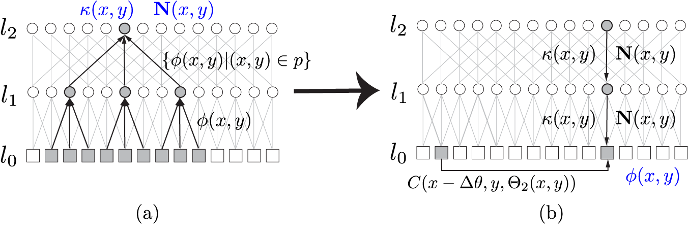
1. Upward pass: Updating local disparity messages. Patch validities and disparity messages are updated in an upward pass, with messages passing from children to parents, as depicted in black in Fig. 4 and in Fig. 5(a). For validities, each patch computes an internal pair of binary values indicating, respectively, whether it contains a foreground pixel and a visible-background pixel. With this notation, Eq. 8 becomes , and computing for is trivial using lateral connections. For patches in higher levels, , we sequentially compute
| (14) |
with the logical OR operator.
Local disparity messages are updated by first computing
| (15) |
at patches and then sequentially computing
| (16) |
for .
2. Downward pass: Updating consensus. Consensus values are updated using messages from parents to children in a downward pass, as depicted in blue in Fig. 4 and in Fig. 5(b). Each patch computes
| (17) |
and passes and to its children. The consensus at each pixel is the result at the pixel level:
| (18) |
3. Updating global shapes and boundary. Global shapes can be computed cooperatively in by first computing local correlation matrix
| (19) |
and cross-correlation -vector
| (20) |
with -vector in each patch separately, and then updating using Tron and Vidal’s consensus averaging algorithm [38] with the lateral connections in .
VII Experiments
Datasets. Existing stereo benchmarks do not include two-layer, figure-ground scenes, so we curate our own using four photographic crops from Middlebury 2006 [13] and eleven renderings from Falling Things [14], shown in Fig. 8. The latter includes ground-truth foreground boundaries, and we manually annotate them in the former. We additional use three multi-layer scenes from Middlebury 2006 [13] to examine the model’s behavior when a scene differs significantly from a two-layer one (Fig. 10).
Matching and boundary signals. Our model can use any underlying matching and boundary signals, including those from learned, deep models (e.g., [4, 39, 40]). Here we choose to use simpler, weaker signals to focus the burden on our optimization and to ensure we are providing a conservative estimate of achievable performance.
We use absolute difference of intensity for matching, . We generate the monocular boundary cost from Eq. 3 using edge maps created by convolving a Sobel filter with each input image, thresholding the responses, and converting the resulting binary edge maps to distance functions and where at detected edges and away from edges. For the occlusion boundary cost , we compute the epipolar gradient magnitude , threshold the result, and convert the binary volumetric function to a distance function where at the detected boundaries. We linearly normalize the values in each of , and to be in the range . The thresholds for monocular edge maps and occlusion boundary maps vary slightly from scene to scene and are optimized for each scene.


| Image | 1 | 2 | 3 | 4 | 5 | 6 | 7 | 8 | 9 | 10 | 11 | 12 | 13 | 14 | 15 | Avg occlusion F1 | |
|---|---|---|---|---|---|---|---|---|---|---|---|---|---|---|---|---|---|
| SGM [41] | 0.39 | 0.38 | 0.42 | 0.65 | 0.23 | 0.32 | 0.00 | 0.02 | 0.58 | 0.67 | 0.04 | 0.87 | 0.27 | 0.61 | 0.72 | 0.41 | |
| BM-LR | 0.37 | 0.34 | 0.48 | 0.70 | 0.01 | 0.22 | 0.00 | 0.00 | 0.57 | 0.72 | 0.18 | 0.92 | 0.07 | 0.59 | 0.44 | 0.37 | |
| KZ [21] | 0.14 | 0.55 | 0.76 | 0.78 | 0.76 | 0.53 | 0.68 | 0.70 | 0.83 | 0.82 | 0.57 | 0.90 | 0.46 | 0.60 | 0.85 | 0.66 | |
| HSM [24] | 0.55 | 0.63 | 0.98 | 0.62 | 0.49 | 0.31 | 0.04 | 0.60 | 0.64 | 0.83 | 0.18 | 0.87 | 0.23 | 0.70 | 0.90 | 0.57 | |
| Ours | 0.87 | 0.60 | 0.99 | 0.78 | 0.86 | 0.55 | 0.61 | 0.75 | 0.75 | 0.98 | 0.64 | 0.95 | 0.79 | 0.81 | 0.88 | 0.79 |
| Image | 1 | 2 | 3 | 4 | 5 | 6 | 7 | 8 | 9 | 10 | 11 | 12 | 13 | 14 | 15 | Avg bad-4.0 | |
|---|---|---|---|---|---|---|---|---|---|---|---|---|---|---|---|---|---|
| SGM [41] | 13.10 | 21.79 | 43.66 | 10.30 | 10.65 | 29.53 | 8.09 | 11.46 | 17.41 | 8.94 | 8.03 | 19.75 | 14.27 | 14.17 | 32.38 | 17.57 | |
| BM-LR | 19.88 | 30.71 | 36.97 | 9.21 | 12.78 | 32.36 | 13.42 | 13.13 | 22.07 | 15.47 | 7.83 | 16.42 | 17.09 | 17.86 | 45.06 | 20.68 | |
| KZ [21] | 31.26 | 13.15 | 49.97 | 3.84 | 3.53 | 18.86 | 2.10 | 3.22 | 12.52 | 1.62 | 2.57 | 9.99 | 24.60 | 57.40 | 29.05 | 17.58 | |
| HSM [24] | 1.69 | 3.35 | 0.25 | 1.80 | 0.99 | 2.92 | 0.00 | 0.00 | 2.59 | 0.89 | 0.00 | 5.69 | 2.38 | 3.18 | 63.08 | 5.92 | |
| Ours | 0.71 | 24.84 | 7.54 | 8.05 | 0.17 | 30.89 | 0.00 | 1.50 | 41.38 | 1.73 | 0.60 | 10.23 | 3.20 | 32.34 | 77.81 | 16.07 |
Metrics and comparison methods. We measure boundary accuracy using precision and recall—summarized by F1 score—of estimated binary occlusion labels in a region of epipolar pixels around the ground-truth boundary (see Fig. 7). As a secondary comparison, we measure accuracy of estimated disparities in the true, mutually-visible subset of this region, using the fraction of pixels at which the disparity error is greater than four pixels (bad-4.0).
For comparisons, we consider four categories of techniques and select one representative method from each of them:
- 1.
BM-LR: Block matching and pixel-wise winner-take-all, followed by a left-right consistency check (e.g., [42]);
- 2.
SGM: Semi-global matching, based on multi-directional 1D dynamic programming [41];
- 3.
KZ: Graph-cuts with occlusion [21];
- 4.
HSM: A deep CNN model that augments training with fake occlusions [24].
Implementation details. For each input, we manually initialize our model to an elliptical boundary as shown in Figures 8 and 10. We re-initialize to a signed distance function every iterations, and we apply a median filter to after every iteration to eliminate thin structures. Parameters values are: ; ; ; ; and . Our implementation of the alternating descent algorithm and data are open sourced at https://github.com/jialiangw/levelsetstereo.
We use MATLAB 2019b implementations of SGM and BM-LR and the authors’ implementation for KZ and HSM. We use the HSM authors’ weights, trained on a mixture of datasets including Middlebury, and the occlusion geometry discussed in Sec. II to get occlusions.


VII-A Results on two-layer scenes
Our qualitative results on two-layer, figure-ground scenes are shown in Fig. 8, and some comparisons with other methods are shown in Fig. 9. The quantitative results are summarized in Tables I and II. Our model provides the highest boundary accuracy (lowest occlusion F1-score) in all but four scenes, and its disparity error near the boundaries (bad-4.0 error) is better than most. The deep model, HSM, achieves substantially lower disparity error as expected, but its occlusion accuracy is middling. This supports the belief that iterative bottom-up models like ours could complement disparity estimates from deep feed-forward models.
Our model’s least accurate boundaries, meaning those with lowest occlusion F1-score, occur in scenes 2, 6, 7, 9 and 11. The qualitative results in Fig. 8 show that this typically occurs when the foreground or background shape deviates substantially from a quadratic model, as can be seen in scenes 2, 6 and 9. F1-scores in scenes 7 and 11 are low for a different reason: the ground truth contains very few occluded pixels, making F1-score very sensitive to boundary misalignment. Our model also performs poorly in scene 4, where the background regions between the doll’s head and arms are almost entirely occluded or have weak matching cues (especially with our simple matching cost), causing our model not to properly group these regions with the rest of the background.
VII-B Results on more complex scenes
Fig. 10 qualitatively demonstrates how the model behaves for three scenes that deviate substantially from two-layer. Note that rows (3) and (4) depict results for the same scene but with different initializations. In scene (1) there are few boundary occlusion cues, so is roughly constant and the model fits its two quadratic shapes to match monocular color boundaries and minimize matching cost. The predicted boundaries are not meaningful, but the disparity map still provides a coarsened approximation to the ground truth. In scenes (2) and (3), the model’s foreground boundary is more useful but still inaccurate. Row (4) shows that when a scene deviates substantially from two quadratic layers, our method can be sensitive to local minima caused by the boundary cues induced by secondary objects. Here we initialize the boundary to a larger ellipse and find that the model converges to a local minimum caused by the painted color boundaries on the box behind the lampshade. Nonetheless, the converged consensus and the final disparity map still provide a coarsened approximation to the ground truth.
VIII Conclusion
By exploiting occlusion and matching cues on equal footing, our model localizes foreground contours in a variety of bi-layer scenes. The algorithm can be implemented in a cooperative manner, with messages passing along sparse connections between units with different receptive field sizes. It provides promising results despite having only five tunable parameters and using local matching and boundary signals that are as simple as possible.
An algorithm like ours can be used as-is for scenes with isolated foreground objects and for tasks, like grasping, that rely heavily on having an accurate foreground mask. Broadening to general scenes and tasks will require upgrading the underlying matching and boundary signals to more sophisticated (e.g., “deep” [39, 4, 40]) alternatives, and perhaps tuning the parameters jointly by unrolling our model’s iterations in time. It could also be combined with a secondary processing step to recover higher-fidelity disparity details within the two smooth regions (i.e., surface parallax).
Open question include how to increase the number of regions beyond two (e.g., using multi-phase level sets [43]), how to reduce sensitivity with respect to initialization, and how to combine this sort of bottom-up stereo boundary processing with complementary top-down information from deep feed-forward models. Another direction is to explore ways of encoding geometric relationships between smooth layers, such as when planar facets join at a crease. How and whether such relationships are encoded in the human visual system remains a mystery (see [44, 45]) that computational models may help solve.
Appendix A Derivation of update to
The Euler-Langrange equations are
| (22) |
| (23) |
In the last line, we use the property when . This assumes that there are no thin foreground structures that violate the ordering constraints [46], as illustrated using the purple points in Figure 11. Therefore,
| (24) |
The second part of Equation 22 is
| (25) |
Combining Equations (24) and (25) gives
| (26) |
The second Euler-Lagrange equation (23) also has two parts but the second one is zero, so the right side of that equation is
| (27) |
where we assume there are no thin background structures such that the entire background segment is occluded, as depicted by blue points in Figure 11.
Let and sum Equations (26) and (27). We obtain:
| (28) |
where
are the curvature and normal of the foreground boundary contour.
Near the border of the cyclopean visual field , it is possible that is outside of the visual field. When this occurs, we extrapolate the value of from the border for use in Equation 28.
References
- [1] J. Wang and T. Zickler, “Level set stereo for cooperative grouping with occlusion,” arXiv preprint arXiv:2006.16094, 2021.
- [2] J. Wang, “Perceptually-consistent boundaries and shape from stereo occlusions,” PhD dissertation, Harvard University, 2021.
- [3] M. Poggi, F. Tosi, K. Batsos, P. Mordohai, and S. Mattoccia, “On the synergies between machine learning and stereo: a survey,” arXiv:2004.08566, 2020.
- [4] J. Wang and T. Zickler, “Local detection of stereo occlusion boundaries,” in Computer Vision and Pattern Recognition, 2019.
- [5] D. Scharstein, H. Hirschmüller, Y. Kitajima, G. Krathwohl, N. Nešić, X. Wang, and P. Westling, “High-resolution stereo datasets with subpixel-accurate ground truth,” in German conference on pattern recognition. Springer, 2014, pp. 31–42.
- [6] V. Caselles, R. Kimmel, and G. Sapiro, “Geodesic active contours,” in International Journal of Computer Vision. Springer, 1997.
- [7] T. F. Chan and L. A. Vese, “Active contours without edges,” in Transactions on Image Processing, 2001.
- [8] P. N. Belhumeur, “A bayesian approach to binocular steropsis,” in International Journal of Computer Vision, 1996.
- [9] A. F. Bobick and S. S. Intille, “Large occlusion stereo,” International Journal of Computer Vision, 1999.
- [10] J. Wang, D. Glasner, and T. Zickler, “Toward perceptually-consistent stereo: A scanline study,” in International Conference on Computer Vision, 2017.
- [11] R. Deriche, C. Bouvin, and O. D. Faugeras, “Level-set approach for stereo,” in Investigative Image Processing, 1997.
- [12] D. Scharstein and C. Pal, “Learning conditional random fields for stereo,” in Computer Vision and Pattern Recognition, 2007.
- [13] H. Hirschmuller and D. Scharstein, “Evaluation of cost functions for stereo matching,” in Computer Vision and Pattern Recognition, 2007.
- [14] J. Tremblay, T. To, and S. Birchfield, “Falling things: A synthetic dataset for 3D object detection and pose estimation,” in Computer Vision and Pattern Recognition Workshops, 2018.
- [15] R. Szeliski, Computer vision: algorithms and applications. Springer Science & Business Media, 2010.
- [16] I. Tsirlin, L. M. Wilcox, and R. S. Allison, “A computational theory of da Vinci stereopsis,” in Journal of vision. The Association for Research in Vision and Ophthalmology, 2014.
- [17] A. Yezzi and S. Soatto, “Stereoscopic segmentation,” in International Journal of Computer Vision, 2003.
- [18] S. Birchfield and C. Tomasi, “Depth discontinuities by pixel-to-pixel stereo,” International Journal of Computer Vision, vol. 35, no. 3, pp. 269–293, 1999.
- [19] X. Song, X. Zhao, L. Fang, H. Hu, and Y. Yu, “Edgestereo: An effective multi-task learning network for stereo matching and edge detection,” International Journal of Computer Vision, 2020.
- [20] J. Weng, N. Ahuja, T. S. Huang et al., “Two-view matching.” in ICCV, vol. 88, 1988, pp. 64–73.
- [21] V. Kolmogorov and R. Zabih, “Computing visual correspondence with occlusions using graph cuts,” in International Conference on Computer Vision, 2001.
- [22] A. S. Ogale and Y. Aloimonos, “Shape and the stereo correspondence problem,” International Journal of Computer Vision, vol. 65, no. 3, pp. 147–162, 2005.
- [23] K. Yamaguchi, T. Hazan, D. McAllester, and R. Urtasun, “Continuous markov random fields for robust stereo estimation,” in European Conference on Computer Vision, 2012.
- [24] G. Yang, J. Manela, M. Happold, and D. Ramanan, “Hierarchical deep stereo matching on high-resolution images,” in Computer Vision and Pattern Recognition, 2019.
- [25] B. Julesz, Foundations of Cyclopean Perception. University of Chicago Press, 1971.
- [26] T. Darrell and A. Pentland, “Robust estimation of a multi-layered motion representation,” in Proceedings of the IEEE Workshop on Visual Motion. IEEE Computer Society, 1991, pp. 173–174.
- [27] J. Y. Wang and E. H. Adelson, “Layered representation for motion analysis,” in Computer Vision and Pattern Recognition, 1993.
- [28] R. Kumar, P. Anandan, and K. Hanna, “Direct recovery of shape from multiple views: A parallax based approach,” in International Conference on Pattern Recognition, 1994.
- [29] S. Baker, R. Szeliski, and P. Anandan, “A layered approach to stereo reconstruction,” in Computer Vision and Pattern Recognition, 1998.
- [30] M. H. Lin and C. Tomasi, “Surfaces with occlusions from layered stereo,” in Computer Vision and Pattern Recognition, 2003. Proceedings., 2003.
- [31] D. Sun, E. B. Sudderth, and M. J. Black, “Layered image motion with explicit occlusions, temporal consistency, and depth ordering,” in Advances in Neural Information Processing Systems, 2010.
- [32] D. Marr and T. Poggio, “Cooperative computation of stereo disparity,” in Science. American Association for the Advancement of Science, 1976.
- [33] J. Sun, N.-N. Zheng, and H.-Y. Shum, “Stereo matching using belief propagation,” IEEE Transactions on pattern analysis and machine intelligence, vol. 25, no. 7, pp. 787–800, 2003.
- [34] P. F. Felzenszwalb and D. P. Huttenlocher, “Efficient belief propagation for early vision,” in International Journal of Computer Vision, 2006.
- [35] G. Li and S. W. Zucker, “Differential geometric inference in surface stereo,” in IEEE Transactions on Pattern Analysis and Machine Intelligence. IEEE, 2008.
- [36] A. Chakrabarti, Y. Xiong, S. J. Gortler, and T. Zickler, “Low-level vision by consensus in a spatial hierarchy of regions,” in Computer Vision and Pattern Recognition, 2015.
- [37] C. L. Zitnick and T. Kanade, “A cooperative algorithm for stereo matching and occlusion detection,” Transactions on Pattern Analysis and Machine Intelligence, 2000.
- [38] R. Tron and R. Vidal, “Distributed computer vision algorithms through distributed averaging,” in Computer Vision and Pattern Recognition, 2011.
- [39] J. Žbontar and Y. LeCun, “Stereo matching by training a convolutional neural network to compare image patches,” in Journal of Machine Learning Research, 2016.
- [40] S. Xie and Z. Tu, “Holistically-nested edge detection,” in International Conference on Computer Vision, 2015.
- [41] H. Hirschmuller and D. Scharstein, “Evaluation of stereo matching costs on images with radiometric differences,” in Transactions on Pattern Analysis and Machine Intelligence, 2009.
- [42] P. Fua, “A parallel stereo algorithm that produces dense depth maps and preserves image features,” Machine vision and applications, 1993.
- [43] L. A. Vese and T. F. Chan, “A multiphase level set framework for image segmentation using the Mumford and Shah model,” in International Journal of Computer Vision, 2002.
- [44] K. Nakayama and S. Shimojo, “Experiencing and perceiving visual surfaces,” in Science, 1992.
- [45] W. H. Ehrenstein and B. J. Gillam, “Early demonstrations of subjective contours, amodal completion, and depth from half-occlusions:“stereoscopic experiments with silhouettes” by Adolf von Szily (1921),” in Perception, 1998.
- [46] A. L. Yuille and T. Poggio, “A generalized ordering constraint for stereo correspondence,” Tech. Rep., 1984.