Generalized Minimum Error Entropy for Adaptive Filtering

Renyi’s seminal work on information theory is called Renyi’s ${\mu}$ entropy:

Here, ${\mu\left({\mu\neq 1,\mu>0}\right)}$ represent the order of Renyi’s entropy. The ${\mu}$ information potential (${\mu}$ IP) ${{V_{\mu}}\left(e\right)}$ of continuous variables is expressed as

Here ${p\left(\cdot\right)}$ denotes the probability density function (PDF) with respect to ${e}$, and ${{\text{E}}\left[\cdot\right]}$ stands for the expectation operator. In fact, PDF ${p\left(x\right)}$ is always estimated utilizing Parzen’s window strategy:

where ${{{\text{G}}_{\sigma}}(x)=\left({1/\sqrt{2\pi}\sigma}\right)\exp\left({-{x^{2}}/2{\sigma^{2}}}\right)}$ stands for the Gaussian kernel function, and ${\sigma}$ stands for kernel bandwidth, and ${\left\{{{e_{i}}}\right\}_{i=1}^{L}}$ are ${L}$ error samples. Combining (2) and (3), the estimation of the quadratic IP ${{V_{2}}\left(e\right)}$ can be obtained

The kernel function of conventional error entropy is always a Gaussian kernel function, however, it is not necessarily the best option. The GGD function is a widely known extension of Gaussian density function [38]:

In Eq. (5), parameter ${\alpha}$, referred to as a shape parameter, denotes the exponential rate of decay. Parameter ${\beta}$, often called scale parameter, denotes the dispersion of the distribution. When shape parameter is set to 1 or 2, the GGD distribution turns to Laplacian or Gaussian distribution. Fig. 1 shows the GGD distribution with different shape parameters. According to Fig. 1, it is obvious that the smaller the value of ${\alpha}$, the heavier the tail of the GGD distribution shape. When it satisfies ${\alpha\to\infty}$, the GGD distribution turns to the uniform distribution. When it satisfies ${\alpha\to 0{\text{ + }}}$, GGD distribution turns to ${\delta}$-distribution.

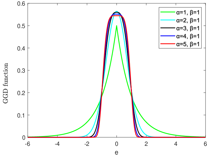
In our study, the GGD function is treated as the new kernel function of error entropy, and we define IP

where

In practical application, only a finite number of error set ${\left\{{{e_{i}}}\right\}_{1}^{L}}$ can be obtained. Substituting (7) into (6) yields (${\mu{\text{ = }}2}$)

According to (8), the IP can be calculated by using double summation method. This method causes a huge computational burden to get the IP, especially for large data sets. Therefore, on the basis of the generalized error entropy, we refer to previous studies [39] to propose quantized generalized error entropy

Here, where quantization operator [39] ${{\text{Q}}\left[{{e_{j}},\gamma}\right]\in C}$ (${\gamma}$ denotes the quantization threshold) is used to obtain a codebook ${C=\left\{{{c_{1}},{c_{2}},\cdots{c_{H}}\in{\mathbb{R}^{1}}}\right\}}$ (in general ${H\leqslant L}$). ${{H_{h}}}$ denotes the number of error set that are quantized to the code, ${\hat{p}_{\alpha,\beta}^{Q}\left(e\right)=(1/L)\sum\nolimits_{h=1}^{H}{{H_{h}}{{\text{G}}_{\alpha,\beta}}(e-{c_{h}})}}$ is the PDF estimator based on the quantized error samples. Obviously, one has ${L=\sum\nolimits_{h=1}^{H}{{H_{h}}}}$ and ${\int{\hat{p}_{\alpha,\beta}^{Q}}\left(e\right)de=1}$.

Generalized error entropy is similar to error entropy and can also serve as a criterion in estimation related problems. For linear adaptive filtering, under the generalized minimum error entropy (GMEE) criterion, the optimal weight vector of adaptive filtering can be calculated through minimizing equation (12):

Under new optimization criterion (12), We derive a kind of random gradient-based novel adaptive filtering, and call it GMEE algorithm

with

where ${\operatorname{sign}(\cdot)}$ is SIGN function, ${\eta>0}$ is the step-size.

Similar to the derivation of (12) and (13), we can obtain the cost function based on quantized generalized error entropy (9)

and an updated form of the weight vector

Here, ${{{\boldsymbol{\Lambda}}_{n}}=\left[{\begin{array}[]{*{20}{c}}{{a_{n}}}&{{a_{n+1}}}&\cdots&{{a_{n+L-1}}}\end{array}}\right]\in{\mathbb{R}^{1\times L}}}$ is a vector with

The computational burden of the GMEE algorithm can be effectively reduced by quantifying the set of errors ${\left\{{{e_{i}}}\right\}_{i=1}^{L}}$, and the computational complexity and performance of the proposed QGMEE are shown in Sections IV and V, respectively.

In this subsection, a new kernel adaptive filtering algorithm based on GMEE criterion. The kernel adaptive filtering algorithms are efficient online learning methods for nonlinear and nonstationary system modeling, which are linear adaptive algorithms in kernel space and virtually nonlinear algorithms in original space [43]. The kernel adaptive filtering algorithm consists of two main types of algorithms, kernel least mean square (KLMS) and kernel recursive least squares (KRLS). The KRLS algorithms outperform KLMS algorithms at the cost of higher computational complexity, and kernel recursive minimum error entropy (KRMEE) [44] and kernel recursive maximum correntropy (KMC) [45] are good examples. The derivation of the new kernel adaptive filtering algorithm is shown below.

The cost function, based on GMEE criterion, of kernel adaptive filtering is given as following:

and the gradient of (19) with respect to ${{\boldsymbol{w}}}$ can be obtain

with

Here, ${{\gamma_{1}}}$ represents regularization factor, ${{{e_{i}}}}$ is error.

Setting ${\partial J\left({\boldsymbol{w}}\right)/\partial{\boldsymbol{w}}=0}$, and one can obtain

with

A new KRLS type algorithm based on GMEE (KRGMEE) can be obtained from the derivation above, and its pseudo-code is displayed in Algorithm 1.

The equation (13) it is further formulated as below

where ${{{\boldsymbol{\tilde{w}}}_{n}}={{\boldsymbol{w}}_{s}}-{{\boldsymbol{w}}_{n}}}$, and priori and posteriori errors of the GMEE algorithm are defined by

and ${{{\boldsymbol{\varepsilon}}_{a;n}}{\text{ = }}\left[{\begin{array}[]{*{20}{c}}{{{\boldsymbol{e}}_{a;n}}}&{{{\boldsymbol{e}}_{a;n+1}}}&\cdots&{{{\boldsymbol{e}}_{a;n+L-1}}}\end{array}}\right]}$.

Some expressions can obtain for simplicity

Moreover, by combining the defining (28) and (29), one can obtain

Left multiply both sides of (27) by ${{\boldsymbol{U}}_{n}^{\text{T}}}$, and one can obtain

we can further get the following expression with assumption that matrix ${{{\boldsymbol{U}}_{n}^{\text{T}}{{\boldsymbol{U}}_{n}}}}$ is invertible

Substituting (32) into (27), and one can obtain

We then square both sides to get

This yields, after some straightforward manipulations, the relation

From (35), when it meets the conditions ${{\text{E}}\left[{{{\left\|{{{{\boldsymbol{\tilde{w}}}}_{n+1}}}\right\|}^{2}}}\right]={\text{E}}\left[{{{\left\|{{{{\boldsymbol{\tilde{w}}}}_{n}}}\right\|}^{2}}}\right]}$, one can obtain

According to assumption A2, the equation (36) can be rewritten as

According to assumption A2, it is easy to obtain

then one can obtain

When time point ${n\to\infty}$, one can get ${{e_{n}}\to{v_{n}}}$, then matrices ${{{{\boldsymbol{P}}_{n}}}}$ and ${{{{\boldsymbol{Q}}_{n}}}}$ can be written as

with

When the system is ergodic in a general sense, (41) can be further written as

It is obvious that if step-size ${\eta}$ satisfies (39), then the sequence of ${{\text{E}}\left[{{{\left\|{{{{\boldsymbol{\tilde{w}}}}_{n}}}\right\|}^{2}}}\right]}$ is convergent.

Similar to the derivation above (the stability analysis of the QGMEE algorithm is very similar to that of the GMEE algorithm, so we present the convergence conditions of the QGMEE algorithm directly), one can obtain the convergence condition of the QGMEE algorithm as the following form

with

where ${{v_{h}}=Q\left[{{e_{j}},\gamma}\right],(h=1,2,\cdots,H).}$ One can obtain an approximation of the critical value of the step size of the QGMEE algorithm by calculating Eqs. (43) and (44).

To investigated the steady-state behavior of GMEE algorithm, we start from the averaged relation (35). It is assumed that the GMEE algorithm is stable, and it will reach a steady state when it meets that

One can further obtain from (35)

Left multiplying both sides of (46) by left inverse of ${{\text{E}}\left[{\left({{{\boldsymbol{P}}_{n}}-{{\boldsymbol{Q}}_{n}}}\right)}\right]}$:

and we obtain

Substituting (38) into (48), one can obtain

Assuming that the proposed adaptive filter is stable, we can get the steady-state excess mean square error (EMSE) of GMEE algorithm.

The steady-state excess mean square error (EMSE) of QGMEE algorithm can be obtain by a similar derivation process as above

When time point ${n\to\infty}$, one can get ${{e_{n}}\to{v_{n}}}$, then matrices ${{{{\boldsymbol{P}}_{n}}}}$ and ${{{{\boldsymbol{Q}}_{n}}}}$ can be computed. Knowing the noise distribution, the theoretical value of the EMSE can be calculated by (50).

As shown in table I, we compare the computational complexities of the proposed algorithms (GMEE and QGMEE) with several adaptive filtering algorithms including LMS, LMF, and GMCC algorithms. The method [40] is utilized to approximate the computational complexity of the algorithm, and the results are displayed as follows

From Eq. (52), we can obtain the GMEE algorithm has a slightly higher computational complexity compared with LMS, LMF, and GMCC algorithms. In general, the number of real-valued code words ${H}$ is much less than the length of the sliding window ${L}$, as it shown in Table 2. We can infer that the adoption of the quantization mechanism can effectively reduce the computational complexity of the GMEE algorithm, and which has only a minimal negative impact on the performance of the GMEE algorithm (detailed simulations are shown in Section V).

References

- [1] W. Yin, Y. Wei, T. Liu, and Y. Wang, “A novel orthogonalized fractional order filtered-x normalized least mean squares algorithm for feedforward vibration rejection,” Mechanical Systems and Signal Processing, vol. 119, pp. 138–154, 2019.
- [2] P. Song and H. Zhao, “Filtered-x least mean square/fourth (fxlms/f) algorithm for active noise control,” Mechanical Systems and Signal Processing, vol. 120, pp. 69–82, 2019.
- [3] L. Tan and J. Jiang, “Active control of impulsive noise using a nonlinear companding function,” Mechanical Systems and Signal Processing, vol. 58-59, pp. 29–40, 2015.
- [4] C. Huang, W. Ding, R. Gao, P. Mei, and H. R. Karimi, “Distributed state-of-charge estimation for lithium-ion batteries with random sensor failure under dynamic event-triggering protocol,” Information Fusion, vol. 95, pp. 293–305, 2023.
- [5] S. H. Pauline, D. Samiappan, R. Kumar, A. Anand, and A. Kar, “Variable tap-length non-parametric variable step-size nlms adaptive filtering algorithm for acoustic echo cancellation,” Applied Acoustics, vol. 159, p. 107074, 2020.
- [6] P. Wen, J. Zhang, S. Zhang, and D. Li, “Augmented complex-valued normalized subband adaptive filter: Algorithm derivation and analysis,” Journal of the Franklin Institute, vol. 356, no. 3, pp. 1604–1622, 2019.
- [7] Y. Bai, X. Wang, X. Jin, T. Su, J. Kong, and B. Zhang, “Adaptive filtering for mems gyroscope with dynamic noise model,” ISA Transactions, vol. 101, pp. 430–441, 2020.
- [8] B. Chen, L. Xing, H. Zhao, N. Zheng, and J. C. Prı´ncipe, “Generalized correntropy for robust adaptive filtering,” IEEE Transactions on Signal Processing, vol. 64, no. 13, pp. 3376–3387, 2016.
- [9] A. Cichocki and S.-i. Amari, Adaptive blind signal and image processing: learning algorithms and applications. John Wiley & Sons, 2002.
- [10] G. Wang, R. Xue, and J. Zhao, “Switching criterion for sub-and super-gaussian additive noise in adaptive filtering,” Signal Processing, vol. 150, pp. 166–170, 2018.
- [11] A. H. Sayed, Fundamentals of adaptive filtering. John Wiley & Sons, 2003.
- [12] S. S. Haykin, B. Widrow, and B. Widrow, Least-mean-square adaptive filters. Wiley Online Library, 2003, vol. 31.
- [13] W. Wang, H. Zhao, and B. Chen, “Bias compensated zero attracting normalized least mean square adaptive filter and its performance analysis,” Signal Processing, vol. 143, pp. 94–105, 2018.
- [14] M. S. E. Abadi, S. Z. Mousavi, and A. Hadei, “Variable step-size block least mean square adaptive filters,” in First International Conference on Industrial and Information Systems, 2006, pp. 593–595.
- [15] S. Cheng, Y. Wei, Y. Chen, S. Liang, and Y. Wang, “A universal modified lms algorithm with iteration order hybrid switching,” ISA Transactions, vol. 67, pp. 67–75, 2017.
- [16] M. Rathod, V. Patel, and N. V. George, “Generalized spline nonlinear adaptive filters,” Expert Systems with Applications, vol. 83, pp. 122–130, 2017.
- [17] T. Veerakumar, B. N. Subudhi, and S. Esakkirajan, “Empirical mode decomposition and adaptive bilateral filter approach for impulse noise removal,” Expert Systems with Applications, vol. 121, pp. 18–27, 2019.
- [18] P. I. Hubscher and J. C. M. Bermudez, “An improved statistical analysis of the least mean fourth (lmf) adaptive algorithm,” IEEE transactions on Signal Processing, vol. 51, no. 3, pp. 664–671, 2003.
- [19] S.-C. Pei and C.-C. Tseng, “Least mean p-power error criterion for adaptive fir filter,” IEEE Journal on Selected Areas in Communications, vol. 12, no. 9, pp. 1540–1547, 1994.
- [20] J. Chambers, O. Tanrikulu, and A. Constantinides, “Least mean mixed-norm adaptive filtering,” Electronics letters, vol. 30, no. 19, pp. 1574–1575, 1994.
- [21] J. Chambers and A. Avlonitis, “A robust mixed-norm adaptive filter algorithm,” IEEE Signal Processing Letters, vol. 4, no. 2, pp. 46–48, 1997.
- [22] Y. Zou, S.-C. Chan, and T.-S. Ng, “Least mean m-estimate algorithms for robust adaptive filtering in impulse noise,” IEEE Transactions on Circuits and Systems II: Analog and Digital Signal Processing, vol. 47, no. 12, pp. 1564–1569, 2000.
- [23] S.-C. Chan and Y.-X. Zou, “A recursive least m-estimate algorithm for robust adaptive filtering in impulsive noise: fast algorithm and convergence performance analysis,” IEEE Transactions on Signal Processing, vol. 52, no. 4, pp. 975–991, 2004.
- [24] X. Zhang, K. Li, Z. Wu, Y. Fu, H. Zhao, and B. Chen, “Convex regularized recursive maximum correntropy algorithm,” Signal Processing, vol. 129, pp. 12–16, 2016.
- [25] B. Chen, X. Wang, N. Lu, S. Wang, J. Cao, and J. Qin, “Mixture correntropy for robust learning,” Pattern Recognition, vol. 79, pp. 318–327, 2018.
- [26] W. Wang, H. Zhao, K. Doğançay, Y. Yu, L. Lu, and Z. Zheng, “Robust adaptive filtering algorithm based on maximum correntropy criteria for censored regression,” Signal Processing, vol. 160, pp. 88–98, 2019.
- [27] S. Peng, B. Chen, L. Sun, W. Ser, and Z. Lin, “Constrained maximum correntropy adaptive filtering,” Signal Processing, vol. 140, pp. 116–126, 2017.
- [28] J. C. Principe, Information theoretic learning: Renyi’s entropy and kernel perspectives. Springer Science & Business Media, 2010.
- [29] X. Fan, G. Wang, J. Han, and Y. Wang, “A background-impulse kalman filter with non-gaussian measurement noises,” IEEE Transactions on Systems, Man, and Cybernetics: Systems, vol. 53, no. 4, pp. 2434–2443, 2022.
- [30] B. Chen, L. Xing, N. Zheng, and J. C. Principe, “Quantized minimum error entropy criterion,” IEEE transactions on neural networks and learning systems, vol. 30, no. 5, pp. 1370–1380, 2018.
- [31] J. He, G. Wang, X. Zhang, H. Wang, and B. Peng, “Maximum total generalized correntropy adaptive filtering for parameter estimation,” Signal Processing, vol. 203, p. 108787, 2023.
- [32] J. He, G. Wang, K. Cao, H. Diao, G. Wang, and B. Peng, “Generalized minimum error entropy for robust learning,” Pattern Recognition, vol. 135, p. 109188, 2023.
- [33] J. He, G. Wang, H. Yu, J. Liu, and B. Peng, “Generalized minimum error entropy kalman filter for non-gaussian noise,” ISA transactions, vol. 136, pp. 663–675, 2023.
- [34] B. Chen, Y. Zhu, and J. Hu, “Mean-square convergence analysis of adaline training with minimum error entropy criterion,” IEEE transactions on neural networks, vol. 21, no. 7, pp. 1168–1179, 2010.
- [35] Z. Li, L. Xing, and B. Chen, “Adaptive filtering with quantized minimum error entropy criterion,” Signal Processing, vol. 172, p. 107534, 2020.
- [36] S. Peng, W. Ser, B. Chen, L. Sun, and Z. Lin, “Robust constrained adaptive filtering under minimum error entropy criterion,” IEEE Transactions on Circuits and Systems II: Express Briefs, vol. 65, no. 8, pp. 1119–1123, 2018.
- [37] J. He, G. Wang, B. Peng, Q. Sun, Z. Feng, and K. Zhang, “Mixture quantized error entropy for recursive least squares adaptive filtering,” Journal of the Franklin Institute, 2021.
- [38] M. K. Varanasi and B. Aazhang, “Parametric generalized gaussian density estimation,” The Journal of the Acoustical Society of America, vol. 86, no. 4, pp. 1404–1415, 1989.
- [39] B. Chen, L. Xing, N. Zheng, and J. C. Príncipe, “Quantized minimum error entropy criterion,” IEEE Transactions on Neural Networks and Learning Systems, vol. 30, no. 5, pp. 1370–1380, 2019.
- [40] B. Chen, X. Liu, H. Zhao, and J. C. Principe, “Maximum correntropy kalman filter,” Automatica, vol. 76, pp. 70–77, 2017.
- [41] G. Wang, B. Chen, X. Yang, B. Peng, and Z. Feng, “Numerically stable minimum error entropy kalman filter,” Signal Processing, vol. 181, p. 107914, 2021.
- [42] F. Ma, J. He, and X. Zhang, “Robust kalman filter algorithm based on generalized correntropy for ultra-wideband ranging in industrial environment,” IEEE Access, vol. 7, pp. 27 490–27 500, 2019.
- [43] Y. Engel, S. Mannor, and R. Meir, “The kernel recursive least-squares algorithm,” IEEE Transactions on Signal Processing, vol. 52, no. 8, pp. 2275–2285, 2004.
- [44] G. Wang, X. Yang, L. Wu, Z. Fu, X. Ma, Y. He, and B. Peng, “A kernel recursive minimum error entropy adaptive filter,” Signal Processing, vol. 193, p. 108410, 2022.
- [45] Z. Wu, J. Shi, X. Zhang, W. Ma, and B. Chen, “Kernel recursive maximum correntropy,” Signal Processing, vol. 117, pp. 11–16, 2015.