Exploring tidal obliquity variations with SMERCURY-TJournal: PSJ
Abstract
We introduce our new code, SMERCURY-T, which is based on existing codes SMERCURY (Lissauer et al. 2012) and Mercury-T (Bolmont et al. 2015). The result is a mixed-variable symplectic N-body integrator that can compute the orbital and spin evolution of a planet within a multi-planet system under the influence of tidal spin torques from its star. We validate our implementation by comparing our experimental results to that of a secular model. As we demonstrate in a series of experiments, SMERCURY-T allows for the study of secular spin-orbit resonance crossings and captures for planets within complex multi-planet systems. These processes can drive a planet’s spin state to evolve along vastly different pathways on its road toward tidal equilibrium, as tidal spin torques dampen the planet’s spin rate and evolve its obliquity. Additionally, we show the results of a scenario that exemplifies the crossing of a chaotic region that exists as the overlap of two spin-orbit resonances. The test planet experiences violent and chaotic swings in its obliquity until its eventual escape from resonance as it tidally evolves. All of these processes are and have been important over the obliquity evolution of many bodies within the Solar System and beyond, and have implications for planetary climate and habitability. SMERCURY-T is a powerful and versatile tool that allows for further study of these phenomena.
Keywords:
Exoplanet dynamics - Astrobiology - Habitable planets - Computational methodsI Introduction
Planetary obliquity is a fundamental parameter that factors into the assessment of a planet’s habitability. The obliquity of a planet, or axial tilt, is the angle between the planet’s spin axis and orbit normal. Together, the value of obliquity and its evolution over time determines the nature of the planet’s seasons (Williams & Kasting 1997; Williams & Pollard 2003; Kilic et al. 2017; Kane & Torres 2017; Kang 2019), atmospheric and oceanic processes (Kilic et al. 2018; Guendelman & Kaspi 2019; Dong et al. 2019; Olson et al. 2020), and ultimately its climatic stability (Milanković 1998; Armstrong et al. 2014; Spiegl et al. 2015; Deitrick et al. 2018b; Colose et al. 2019). Various studies investigated the obliquity evolution of bodies in the Solar System as well as exoplanets for purposes such as gaining insights into their dynamical history, making predictions for the future, or even judging their potential for habitability.
Many processes can contribute to alter a planet’s obliquity over time. Constant torques exerted on a planet’s equatorial bulge by its planetary neighbors in addition to the regular precessional motion of the planet’s orbit plane set a range of benign obliquity variations. On the other hand, a planet can experience large obliquity variations of many tens of degrees if it enters into a secular spin-orbit resonance. Such a resonance occurs when a planet’s spin-axis precession becomes commensurate with a driving eigenfrequency of its orbital precession (Colombo 1966; Peale 1969; Henrard & Murigande 1987). The resultant obliquity variations of this resonance depend on the amplitude of the orbital mode in addition to the planet’s proximity to the resonance center. Provided that a planet resides within a spin-orbit resonance, its resonant angle, , will typically librate about 0 (the stable Cassini States 1 and 2 or the unstable Cassini State 4) or 180 degrees (Cassini State 2, stable), where is the planet’s spin precession angle that defines the azimuthal orientation of the planet’s spin vector and is the phase angle of the orbital precession mode (Deitrick et al. 2018a; Saillenfest et al. 2019; Su & Lai 2020). Furthermore, in the case that the widths of multiple spin-orbit resonances overlap, a planet’s spin axis can be subject to chaotic evolution in which its obliquity swings across a wide range of values. Mars is the poster child for this chaotic behavior, as its obliquity swings from (Laskar & Robutel 1993b; Touma & Wisdom 1993; Laskar et al. 2004b; Li & Batygin 2014). The Earth would suffer a similar fate if not for the Moon’s help in speeding up the Earth’s spin-axis precession enough so that the Earth peacefully resides outside of the chaotic region (Laskar et al. 1993a; Laskar et al. 2004a; Brasser & Walsh 2011).
Considering the working parts that contribute to this resonance, rhythmic gravitational tugs from neighboring planets drive orbital precession while torques from the planet’s star and moons fuel its spin precession. The rate of a planet’s spin precession obeys
| (1) |
where is the planet’s obliquity, and is its orbital eccentricity. In the case of a moonless planet, the precession constant, , goes as
| (2) |
Here is the planet’s mean motion, its spin rate, its oblateness coefficient, and is its normalized polar moment of inertia (this expression is approximate, based on the assumption that the planet’s dynamical ellipticity is roughly proportional to ) (Laskar & Robutel 1993b; Li & Batygin 2014; Quarles et al. 2020).
The status of a planet’s presence within a spin-orbit resonance can change with time. For instance, although the Earth rests easy now, it may have crossed a high-order resonance just a few million years ago (Laskar et al. 1993a; Laskar et al. 2004a). Change can be brought on by a variety of processes, such as those that shift the location and amplitudes of potentially resonant orbital frequencies. Planetary orbital migration mechanisms are one such way to achieve these shifts (Brasser & Lee 2015; Vokrouhlický & Nesvorný 2015; Millholland & Laughlin 2019). In a similar vein, the works of Saillenfest et al. 2020, Saillenfest et al. 2021a, and Saillenfest, Melaine et al. 2021 studied the past and future influence that satellite migration may have had on the obliquity evolution of Jupiter and Saturn. Millholland & Batygin 2019 and Su & Lai 2020 studied another mechanism in which a shrinking protoplanetary disk could cause sweeping spin-orbit resonances to influence the obliquity distribution of newly formed protoplanets. Another study applied this concept to Uranus’s circumplanetary disk to attempt to infer its dynamical history (Rogoszinski & Hamilton 2020).
Alternatively, a planet can be driven into or out of a spin-orbit resonance by processes that alter its spin precession rate (Equation 1). Tidal spin torques are one mechanism that can dynamically shape the fate of a planet’s spin state over time. The tidal friction generated from a system’s star pulling on the equatorial bulges of a planet will slowly drive it toward tidal equilibrium, in which its obliquity will typically increase followed by a gradual decline to a small values, while its spin rate undergoes rotation braking until its spin period becomes synchronous with its orbital period (or pseudo-synchronous for eccentric orbits). This journey amounts to a constant decline in a planet’s precession constant and consequently its spin-precession rate over time, allowing for opportunities to encounter spin-orbit resonances as time goes on. Tidal spin torques can drive a planet’s spin axis to traverse parameter space and undergo scenarios such as spin-orbit resonance crossings, captures, or even traverses of chaotic resonance regions. Since the magnitude of the tidal force decays roughly as with distance, this process is likely especially important for planets in close proximity to their star. The Earth will likely undergo chaotic obliquity variations itself in a few billion years after entering the chaotic zone thanks to its decaying rotation rate (Neron de Surgy & Laskar 1997).
We introduce SMERCURY-T (Kreyche 2021), a joining of the existing code SMERCURY (Lissauer et al. 2012) with elements from Mercury-T (Bolmont et al. 2016) so that we can investigate these dynamic tidal spin phenomena and build a more complete picture of planetary spin dynamics. While SMERCURY utilizes its implementation of the spin Hamiltonian from Touma & Wisdom 1994 to accurately compute the orbital and rotational dynamics of a planetary system due to N-body interactions, it is not equipped to compute tidal evolution. On the other hand, Mercury-T is capable of computing the tidal evolution of a system but limits the study planetary spin evolution by neglecting planet-planet cross terms in its spin calculations. In addition, Mercury-T lacks a scheme to efficiently explore parameter space like the “ghost planet” scheme featured in the SMERCURY-T code (discussed in Section II.1). Similar open-source codes such as Posidonius (Blanco-Cuaresma & Bolmont 2017) and VPLanet (Barnes et al. 2020) are also guilty of these charges. We bridge this gap by branching SMERCURY-T from SMERCURY to include modifications that allow for the complete simultaneous computation of the orbital and spin evolution of a planet while under the effects of stellar tidal spin torques.
In this article, we begin with Section II in which we describe the SMERCURY-T code and discuss our implementation of its new modules. Following that, in Section III we perform several experiments that demonstrate the phenomena of spin-orbit resonance crossings, captures, and chaotic crossings which express the versatility of SMERCURY-T as a tool. We conclude in Section IV.
II Methods
II.1 The Base Code
We present our new code, SMERCURY-T, as a modified version of its predecessor, SMERCURY (Lissauer et al. 2012; Barnes et al. 2016; Quarles et al. 2020; Kreyche et al. 2020). SMERCURY is a mixed-variable symplectic N-body integrator which is itself a modified spin-tracking version of the original MERCURY package (Chambers 1999). Just like the code that SMERCURY-T derives from, it is capable of computing the orbital evolution of multiplanet systems while tracking the spin state of one planet and its “ghosts”. The ghost planet scheme entails the simultaneous simulation of massless copies of the spin-tracked planet, in which the user assigns a unique initial spin state to each ghost planet which will evolve while its orbital evolution mimics that of the original planet. This scheme makes SMERCURY-T advantageous over similar codes by allowing for efficient exploration of parameter space, however its present implementation restricts the user to only being able to simulate the spin evolution of one system’s planet at a time. SMERCURY-T is publicly available (Kreyche 2021).
SMERCURY-T treats the spin computation by considering the spin-tracked planet to be an axisymmetric rigid body. Gravitational torques from the planet’s star and neighboring planets exerted on the spin-tracked planet’s equatorial bulge modify its obliquity. When preparing a simulation, we express the planet’s spin rate by assigning it a value for its zonal gravity coefficient according to the Darwin-Radau relation (Hubbard 1984; Murray & Dermott 1999). This takes the form
| (3) |
with , , and as the planet’s spin rate, mass, and equatorial radius, respectively. Here is the universal gravitational constant and the placeholder is short for
| (4) |
where is the planet’s normalized polar moment of inertia. We calculate according to
| (5) |
with as the average density of the planet. We refer to Lissauer et al. 2012 for a more thorough description of this technique.
II.2 Code Modifications
In this section, we describe the modifications that we include within the SMERCURY-T package based on the alterations that we made to the base SMERCURY code. Here we include the details and implementation of the tidal spin torque module and then discuss the results of a test experiment to verify its accuracy. We also discuss our additional inclusion of a general relativity module.
II.2.1 Tidal Spin Torque Module
The most significant inclusion to the SMERCURY-T code is the tidal spin torque module. We follow the methods of Bolmont et al. 2015 and adopt the constant time lag tidal formulation expressed by Leconte et al. 2010 and others (Mignard 1979; Hut 1981; Eggleton et al. 1998), which is valid for arbitrary values of obliquity, spin, and orbital eccentricity. Contrary to the rigid body considerations that we employ for the N-body torque computations, this model assumes that the body is made of a weakly viscous fluid (Alexander 1973). In the future, SMERCURY-T’s modular design makes it simple to implement and explore alternative tidal models. Our approach differs from the aforementioned works in that we neglect orbital tides and consider only the effects of tidal spin torque on the spin-tracked planet from its star. This choice saves valuable computation time, while still allowing for sufficient study of the behavior of planetary spin evolution in most planetary systems except the most compact ones. Readers can refer to Table 2 of Mardling & Lin 2004, or can perform quick calculations with handy equations such as those found in Rodríguez, A. & Ferraz-Mello, S. 2010 to estimate the importance of orbital tides in their desired system. We justify our study of the systems that we consider in Section III by estimating the semi-major axis damping timescale () and eccentricity damping timescale () to be practically infinite for the Earth-mass planet under study compared to our integration time of 4 Gyr. Another consequence of our methodology is that it is technically in violation with the law of conservation of angular momentum, since the spin-tracked planet’s spin angular momentum decays while the system gets nothing back in return. The choice to neglect the effects of this feedback is acceptable for the study of planetary systems since the total angular momentum of the system will always vastly dwarf the the spin-tracked planet’s spin angular momentum.
The task to modify the spin routine of SMERCURY-T to include tidal spin torques is a relatively straight-forward one. Since SMERCURY-T already integrates the summation of all of the torques felt by the spin-tracket planet’s rotational bulge at each time step, all that remains is calculating the additional tidal torque within the routine. From Bolmont et al. 2015, the non-averaged tidal torque felt by a planet from its star goes as
| (6) |
where is the radial vector between the planet at its star, is the planet’s spin vector, is the radial unit vector, is the planet’s velocity vector, is its potential love number of degree 2, is the constant time lag, is the mass of the star, and is the universal gravitational constant. This calculation treats the star as a point mass while the planet is made up of a reduced central point mass with two point mass bulges. Figure 1 from Bolmont et al. 2015 is a useful diagram that demonstrates some of these elements. Converting this result to heliocentric coordinates allows for a final expression that conforms with the requirements of SMERCURY-T’s spin algorithm. Taking the planet’s spin angular momentum as , the adjusted tidal torque is
| (7) |
As the spin-tracked planet’s spin rate damps over time due to the inclusion of the tidal torque, it is necessary to update the planet’s and equatorial radius at each time step to represent the reduction of its equatorial bulge. This is important not only due to the dependence of the strength of the tidal torque on , but even more so due to the sensitive nature of the N-body spin dynamics computations to the value of as the planet’s spin state evolves. We develop a scheme to update these parameters and provide the details in Appendix A. This scheme involves instructing SMERCURY-T to use the value of the planet’s spin angular momentum to solve a cubic equation to ultimately determine new values for and using Equations A6 and 3.
One possible concern with the inclusion of the tidal spin torque module is that there may be scenarios in which the magnitude of the computed tidal torque is so small that it under flows machine precision, causing the planet’s tidal evolution to cease entirely. We solve this issue by implementing a “tidal tolerance” input parameter that the user can specify prior to running a simulation. This parameter is a fractional value that determines a certain threshold after being multiplied by the total spin angular momentum at the current time step. If the tidal torque components exceed this threshold, then they are integrated and added to the spin vector. However, if they fall below the threshold then SMERCURY-T saves their values and adds them to a running total to be checked the next time around. A typical value for the tidal tolerance parameter that we use in this article is .
II.3 Tidal Spin Torque Module Verification
We verify the implementation of the SMERCURY-T tidal spin torque module by simulating and comparing the results of a test system’s tidal evolution to that of a secular code based on the framework of Leconte et al. 2010. The secular code is capable of solving the averaged equations of one planet’s orbital and rotational tidal evolution. However, since SMERCURY-T only accounts for the effects of tidal spin torques, for a fair comparison we hold the orbital elements constant and evolve the secular code solely with the spin equations. We implement the same scheme from Section II.2.1, detailed in Appendix A, into the secular code to similarly update the planet’s equatorial radius at each time step.
The test system that we use here is a one-planet system that consists of the Sun and an Earth-mass planet with an semi-major axis of 0.2 AU and an orbital eccentricity of 0.3. This choice ensures a short integration time and demonstrates the capability of SMERCURY-T to handle large eccentricities. For both simulations, we assign this planet with a polar moment of inertia, average density, initial spin period, initial equatorial radius, potential love number of degree 2, constant time lag, and initial obliquity according to Table 1. We integrate the SMERCURY-T simulation with a time step of 1.6 days ( 5% of the inner-most planet’s orbital period, our usual rule of thumb) and sample at an interval of 1000 years. The time step for the averaged equations of the secular code does not need to be as small, so we proceed with 1000 year increments. We run both simulations for 10 Myr which is more than enough time for the planet to reach tidal equilibrium.
Planet Physical Parameters
| [g/] | [hours] | [km] | [sec] | [deg] | ||
|---|---|---|---|---|---|---|
| 0.3296108 | 5.5136 | 24 | 6378 | 0.305 | 698 | 45 |
Note. — Physical values for the test planet that we describe in Section II.3. Here we list the planet’s moment of inertia (), average density (), initial spin period (), initial equatorial radius (), potential love number of degree 2 (), constant time lag (), and initial obliquity ().
Looking to Figure 1, we show a comparison between the results of the two codes for the spin evolution of the Earth-mass planet due to the effects of tidal spin torques. Examining the evolution of the planet’s obliquity, spin period, equatorial radius, (initially calculated with Equation 3), and spin angular momentum, we show that SMERCURY-T is in good agreement with the secular code. Although there is a slight discrepancy between the extent of the planet’s obliquity values near the peaks of the plot in Figure 1’s upper left panel, each parameter ultimately tracks and converges to the same end value with little difference between the two codes. In summary, we see that tidal spin torques cause the planet to initially experience an increase in its obliquity until its spin rate decays such that the altitudinal component of its spin angular momentum overtakes the azimuthal component, as shown in the upper and lower right panels of Figure 1. From there, its spin period continues to increase while its obliquity declines until it reaches tidal equilibrium when its obliquity is near zero and its spin period is that of its pseudo-synchronous period ( 21 days here). The planet’s equatorial radius shrinks by about 7 km while its reduces considerably.

II.3.1 General Relativity Module
We also incorporate the general relativistic (GR) force due to the post-Newtonian potential into SMERCURY-T as an optional module following section 2.2 of Bolmont et al. 2016. The GR force not only plays an important role with regard to the stability of a planetary system, but we reason that it can also have an indirect influence on planetary obliquity evolution. This influence stems from the GR effect that causes the precession of periapsis of planetary orbits to speed up. Bearing this in mind, GR can indirectly influence planetary obliquity by shifting the potentially resonant orbital eigenfrequencies. While these effects are important to a degree in our own Solar System, they are likely especially important for compact exoplanet systems whose planets reside deep within their star’s gravitational well.
In the spirit of one famous confirmation of Einstein’s general theory of relativity (Einstein 1916), we verify the implementation of our GR module by checking the contribution of GR to the precession of periapsis of our planetary neighbor, Mercury. We compare the results of our SMERCURY-T simulation to that of the measured rate from the MESSENGER spacecraft reported by Park et al. 2017. We obtain an average value of ′′/Julian century over the course of our 1 Myr simulation in which we used a system consisting only of the Sun and Mercury to isolate the effect of GR. Specifically, this value is the difference between Mercury’s precession rate when the GR module was enabled versus another simulation when it was not. Here we set the integration time step to be 5% of Mercury’s orbital period and sampled at 100 year intervals. This value is in good agreement and lies within the error bars of the Park et al. 2017 result.
III Experiments
In this section, we apply the code modifications discussed in Section II.2 to demonstrate the usefulness and versatility of SMERCURY-T as a tool to study planetary spin dynamics. Here we showcase examples of three different scenarios driven by the effects of tidal spin torques: a spin-orbit resonance crossing, a spin-orbit resonance capture, and a chaotic resonance crossing. We enable the general relativity and tidal spin torque modules (“tidal tolerance” set to ) for these experiments with the exception of the initial frequency analysis runs detailed in Sections III.1.1 and III.3.1.
III.1 Spin-orbit Resonance Crossing
III.1.1 Initial Conditions and Pre-analysis
We design an experiment to exemplify the scenario in which tidal spin torques drive a planet to undergo a spin-orbit resonance crossing as its increasing obliquity and spin period cause its precession constant to decline over time. We choose to use a simple toy system consisting of the Sun, an Earth-mass planet initially placed at 0.5 AU, and a Jupiter-mass planet initially placed at 2.5 AU. This choice allows us to study this process appropriately while minimizing the necessary integration time thanks to the stronger presence of tides closer to the Sun. We display the masses and orbital elements of these bodies in Table 2 listed under system E-J, which shows that the Earth-mass planet and Jupiter-mass planet share an initial mutual inclination of .
System Orbital Parameters
| System | Planet | [] | [AU] | [deg] | [deg] | [deg] | [deg] | |
|---|---|---|---|---|---|---|---|---|
| E-J | Earth | 3.003 x | 0.5 | 0 | 1 | 0 | 0 | 0 |
| Jupiter | 9.54244 x | 2.5 | 0 | 0 | 0 | 0 | 0 | |
| E-E-J | Inner Earth | 3.003 x | 0.5 | 0 | 5 | 0 | 0 | 0 |
| Outer Earth | 3.003 x | 0.7 | 0 | 2.5 | 0 | 0 | 0 | |
| Jupiter | 9.54244 x | 3.5 | 0 | 0 | 0 | 0 | 0 |
Note. — Initial values for the plantary mass (), semimajor axis (), eccentricity (), inclination (), argument of periapsis (), longitude of ascending node (), and mean anomomly () for the Earthmoo-Jupiter (E-J) and Earth-Earth-Jupiter (E-E-J) systems that we test in this article. We take the mass of Sun to be 1.98911 kg.
We perform an initial simulation of the E-J system over the course of 10 Myr, sampling on an interval of 1000 years with a numerical time step of 6.46 days ( 5% of the Earth-mass planet’s orbital period). For this part we are only interested in the system’s orbital evolution, so we leave the GR module enabled but disable the tidal spin torque module in the interest of shaving off some computation time. Taking these results, we perform a frequency analysis routine by applying a Frequency Modified Fourier Transform (Šidlichovský & Nesvorný 1996) to the Earth-mass planet’s inclination and eccentricity vectors ([, ] and [, ] respectively). This process extracts the frequencies, amplitudes, and initial phases of the precessional modes that could enter resonance with the Earth-mass planet. First order resonances appear directly in the inclination series. We display these values in Table 3 listed under system E-J. This information allows us to compute both the location of a resonance center and its width enclosed by the separatrix as a function of a planet’s precession constant and obliquity, following the procedure of Saillenfest et al. 2019. The simplicity of the E-J system results in the single dominant mode in the inclination series at ′′/yr. This frequency sets the target resonance for the Earth-mass planet in the experiments we describe in Section III.1.2 and III.2.2.
Secular Orbital Frequencies
| Inclination Vector Series | Eccentricity Vector Series | ||||||
|---|---|---|---|---|---|---|---|
| System | [′′/yr] | [deg] | [′′/yr] | [deg] | |||
| E-J | 1 | -22.69 | 871406 | 359.94 | 22.89 | 804.86 | 179.80 |
| 2 | 0.00 | 1221 | 0.00 | 0.03 | 431 | 183.31 | |
| 3 | -22.47 | 183 | 15.31 | -9.11 | 15 | 41.66 | |
| 4 | -22.90 | 170 | 149.56 | -6.23 | 14 | 346.47 | |
| 5 | -22.30 | 102 | 6.21 | -7.45 | 13 | 235.11 | |
| E-E-J | 1 | -10.67 | 3736801 | 359.99 | 30.74 | 704 | 180.09 |
| 2 | -32.25 | 617977 | 359.84 | 0.03 | 617 | 180.22 | |
| 3 | -3.97 | 8169 | 0.09 | 12.59 | 53 | 2.33 | |
| 4 | -53.83 | 2096 | 179.43 | 9.15 | 14 | 191.46 | |
| 5 | 10.91 | 786 | 358.52 | -98.64 | 8 | 77.37 |
Note. — The results from our Frequency Modified Fourier Transform analysis of the inclination vector ([,]) and the eccentricity vector ([, ]) of the Earth-mass planet in the Earth-Jupiter (E-J) system and the inner Earth-mass planet in the Earth-Earth-Jupiter (E-E-J) system, where is the orbital inclination, is the longitude of ascending node, is the eccentricity, and is the longitude of periapsis. We show the top five values of the frequencies (), amplitudes (), and phases () of the inclination vector, as well as the top five values of the frequencies (), amplitudes (), and phases () of the eccentricity vector.
Targeting the mode, we initialize the Earth-mass planet so that it will begin its tidal evolution just outside of the resonance and cross paths with the resonance center some time later. Therefore we assign it with an initial obliquity of and a precession constant of 60 ′′/yr (using Equation 2 with a spin period of hours and ). These planetary characteristics are not unrealistic, and could be the aftermath of various primordial scenarios such as giant impacts. We set its initial precession angle to be , while we use the same values for its average density, normalized polar moment of inertia, potential love number of degree 2, and constant time lag as found in Table 1. We run this simulation for 4 Gyr and sample every 10,000 years with the same 6.46 day time step.
III.1.2 Results and Discussion
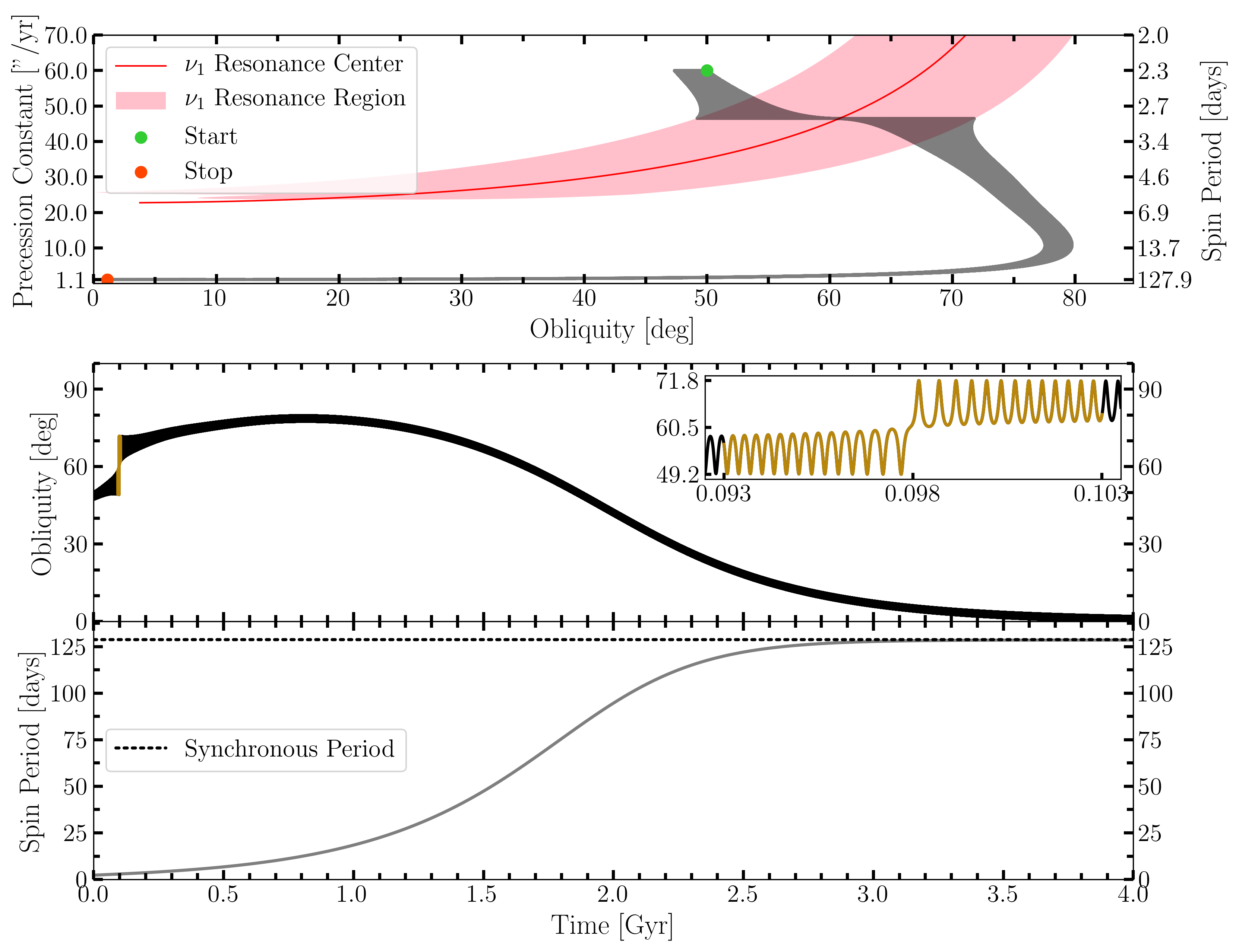
We explore the results of the spin-orbit resonance crossing experiment by looking to Figure 2. We see that the Earth-mass planet begins with an obliquity of and experiences benign obliquity variations of a few degrees that are primarily due to the precessional motion of its orbit. The planet’s precession constant declines while tidal spin torques cause its obliquity to gradually increase as it approaches the resonance. Upon entering the resonance region, the planet’s obliquity swings wildly in the range of . Then, at about 98 Myr into the simulation, the planet’s obliquity suddenly shifts ten degrees as it crosses the resonance center and swings in a new range of . The planet then proceeds to exit the resonance and eventually converges towards tidal equilibrium with the behavior of Cassini State 1, as its obliquity draws near zero and its spin period approaches the synchronous period of days. The nature of these short term obliquity variations as the planet crossed through this resonance during its tidal evolution would likely be harmful toward its prospects for climatic stability and habitability. However, a true assessment of these prospects would require a more complete study that that would explore the application of a climate model. We include an accessory video that shows a time lapse of the crossing event in Figure 3.
Further examination of the resonance crossing event leads us to reason that our choice of the planet’s initial precession angle ensured that it crossed through the resonance’s hyperbolic point (Saillenfest et al. 2021a). In other words, this behavior resulted due to the chance timing and positioning of the planet’s spin axis as its spin precession wound down while the planet crossed the resonance center. Looking to Figure 4, we examine the evolution of the angle centered around the time of the resonance center crossing event at Myr, where is its spin precession angle and is the planet’s longitude of ascending node. We treat this angle as a close approximation of the resonant angle, in which it is diagnostic of the nature of a resonance event. This angle tends to librate about when a planet is captured in resonance in the vicinity of Cassini State 2, otherwise it usually circulates (Deitrick et al. 2018a; Quarles et al. 2020). Here we show that the resonant angle circulates while the planet approaches and moves away from the resonance center while an inflection point appears at the time of the crossing. This behavior reinforces that the planet was never captured into the resonance at any point in time and indeed crossed through its hyperbolic point.

https://github.com/SMKreyche/Kreyche-et-al.-2021-Videos

This angle is diagnostic of the presence of a planet in a spin-orbit resonance. Here the angle circulates with a brief inflection point at the time of the crossing event ( Myr), which indicates that the planet was not captured into the resonance and instead crossed through its hyperbolic point (Saillenfest et al. 2021a).
III.2 Spin-orbit Resonance Capture
III.2.1 Initial Conditions and Pre-analysis
Following the spin-orbit resonance crossing experiment described in Section III.1.1, we now consider an alternative fate for the Earth-mass planet in which it could instead become captured into the spin-orbit resonance. Here we use the exact same initial conditions as the former experiment save one: the initial precession angle. Since the outcome is probabilistic based on the value of the precession angle upon its arrival at the resonance (Henrard 1982; Saillenfest et al. 2021a), we consider a slew of initial precession angles but handpick the case of the Earth-mass planet with an initial precession angle of . We stress here that although this serves our example, this is an atypical pathway toward resonance capture since the planet crosses the resonance “from above” ( proceeds toward unity from greater to smaller values) (Ward & Hamilton 2004; Hamilton & Ward 2004). We simulate this system for 4 Gyr with the same sample rate and time step as the experiment described in Section III.1.1.
III.2.2 Results and Discussion
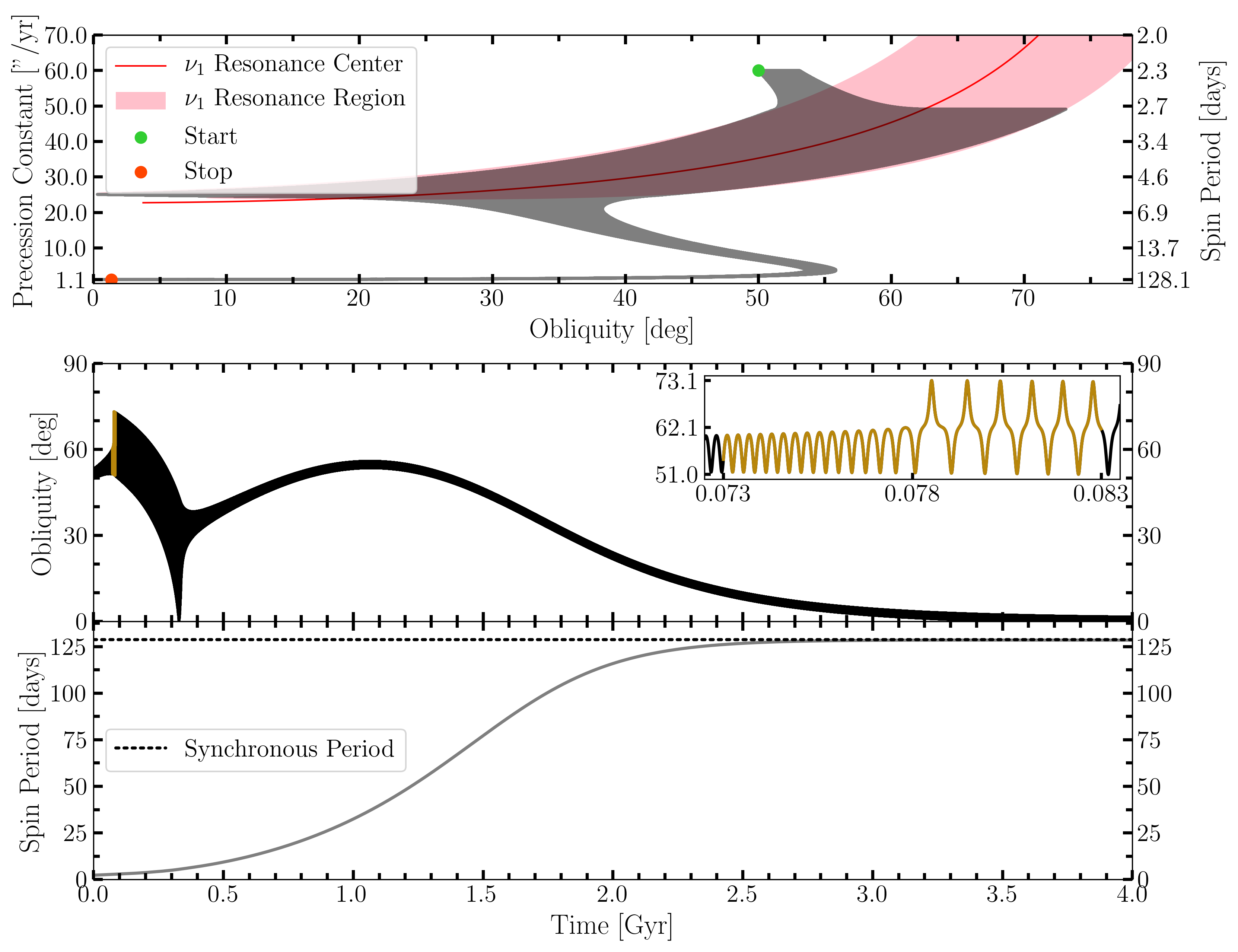
We show the results of the spin-orbit resonance capture experiment by looking to Figure 5. While the Earth-mass planet begins on a track very similar to the crossing experiment described in Section III.1.2, its spin evolution takes a very different path once it enters the resonance. After about 75 Myr into the simulation, the planet crosses the resonance center and is subsequently captured into the resonance. From here, its obliquity experiences large variations of order as it is bound to the follow the track of the resonance’s center as its precession constant declines. Eventually, at around the 350 Myr mark the separatrix of the resonance disappears and the planet exits the resonance. Since the planet’s ride within the resonance led to an inefficient decay of its spin rate, the planet’s obliquity then trends to greater values until peaks at about and then reverses while the planet heads towards tidal equilibrium. The path that the planet’s obliquity ultimately took from start to finish spanned a wide range of values with frequently large obliquity variations over short timescales. Similar to the resonance crossing experiment from Section III.1.2, this behavior would likely be detrimental toward the planet’s prospects for habitability. Look to Figure 6 for a video that shows a time lapse of the initial resonance capture event.
Why did this experiment lead to the Earth-mass planet getting captured into the resonance while the other did not? Recalling that we set this planet to have an initial precession angle of rather than the former experiment’s , we show the temporal evolution of its resonant angle centered around the event in Figure 7. Here we show that prior to the planet’s encounter with the resonance center its resonant angle circulates. However, following the event the resonant angle then librates about , albeit very widely, which is confirmation of the planet’s capture into the resonance. This time, our choice of initial precession angle ensured that the conditions were ripe for capture into the resonance at the time of crossing.

https://github.com/SMKreyche/Kreyche-et-al.-2021-Videos

III.3 Chaotic Crossing
III.3.1 Initial Conditions and Pre-analysis
For our final experiment, we design a scenario that exemplifies a chaotic spin-orbit resonance crossing. The resonance overlap criterion specifies that chaotic regions of parameter space exist in the case that two first-order resonances overlap. Therefore we now consider a system with an additional planet to introduce an additional forced inclination frequency (Saillenfest et al. 2019). We present this system in Table 2 listed under system E-E-J, which shows our new system to consist of the Sun, an Earth-mass planet at 0.5 AU with an inclination of , an Earth-mass planet at 0.7 AU with an inclination of , and a Jupiter-mass planet at 3.5 AU whose orbit sits flat with an inclination of .
We conduct the same frequency analysis as described in Section III.1.1 to extract the information on the relevant modes of this system. We display this information in Table 3 listed under system E-E-J. This time, our inclusion of the additional Earth-mass planet raised the “temperature” of the system, where the inner Earth shows two prominent driving frequencies in its inclination series. The first mode, , has a frequency of ′′/yr and is the primary driver of the inner Earth-mass planet’s orbital precession. The second mode, , has a frequency of ′′/yr with a considerably smaller amplitude. These two frequencies have resonant widths that overlap to form a chaotic region.
We set the inner Earth’s obliquity to and its precession constant to 110 ′′/yr (using Equation 2 with a spin period of hours and ) so that it will begin its tidal evolution just outside of the resonance region and will tidally evolve to cross into the chaotic region. The inner Earth has the same average density, normalized polar moment of inertia, potential love number of degree 2, and constant time lag found in Table 1. We simulate this system over the course of 4 Gyr by sampling on 10,000 year intervals with a 6.46 day time step.
III.3.2 Results and Discussion
We show the results of the chaotic spin-orbit resonance crossing experiment in Figure 8. These results share similarities with Figures 4a and 4b of Neron de Surgy & Laskar 1997 that studied possible chaotic futures for the real Earth. Here the inner Earth begins with an obliquity of and experiences variations of order which are on par with benign variations resulting primarily from the precessional motion of its orbit. As tidal spin torques dampen the planet’s precession constant and push its obliquity towards higher values, the planet crosses into the resonance after about 150 Myr. The resonance excites larger obliquity variations as the planet first crosses the center of the resonance and then into the chaotic overlap region of the and resonance. Chaos ensues, in which the planet’s obliquity violently swings as much as in an unpredictable fashion within the range . This behavior spans from 200-600 Myr into the simulation until the planet finally transitions to crossing through just the resonance and eventually exits to proceed towards tidal equilibrium where its obliquity trends towards zero and its spin period approaches the synchronous period days. Although this planetary system is fictional, its example of chaotic spin evolution implicates the probable catastrophic effects that this behavior could have on the planet’s well-being. Refer to Figure 9 for a video that shows a time lapse of for a period of this chaotic behavior.


https://github.com/SMKreyche/Kreyche-et-al.-2021-Videos
IV Conclusion
In this article we presented our new code, SMERCURY-T, a numerical N-body integrator that is capable of computing the orbital and rotational evolution of a planet under the influence of tidal spin torques. Additionally, we included a module that adds the effects of the general relativistic force to planetary orbital evolution. We verified the proper implementation of these inclusions and showed the potential of SMERCURY-T as a powerful and versatile tool that is capable of tackling a variety of problems.
We used SMERCURY-T to perform a series of experiments to investigate different phenomena that a planet could experience due to the effects of tidal spin torques. These processes are likely important to the long-term dynamics of many planets. The spin-orbit resonance crossing and capture experiments demonstrated the possibility that a planet can take vastly different pathways which are determined purely by its initial conditions. While the resonance crossing experiment showed an example in which tidal spin torques drew a planet to encounter a spin-orbit resonance followed by an abrupt kick to its obliquity, the resonance capture experiment instead resulted in the planet engaging in a stable libration within the resonance while it was transported toward lower obliquity for a period of time. We also showed the results of the crossing of a chaotic region formed by the overlap of two spin-orbit resonances. The large chaotic swings of the planet’s obliquity are familiar and consistent with the dynamics of some of the bodies in our own Solar System.
Although the planetary systems that we considered in this article were fictional, our general study of the nature of tidal obliquity evolution demonstrates possible scenarios that may have implications for the past, present, and future dynamics of planetary obliquity evolution. Knowing that the climatic stability and consequently, the habitability of planet, is strongly related to the nature of its obliquity evolution, understanding the dynamic role that tidal spin torques can play is critical knowledge. Large and rapid obliquity variations like those that we observed in our experiments would likely be detrimental toward a planet’s climatic stability, and therefore its prospects for habitability. Although we did not investigate this claim in this article, an interesting avenue for future work could involve the application of a climate model to explore the potentially destructive consequences of these evolutionary pathways.
For future work, SMERCURY-T can serve as a tool to further explore tidal obliquity evolution and seek answers to questions about the planets in our Solar System and beyond. The effects of tidal spin torques are especially relevant to planets that are in close proximity to their star, such our own system’s inner terrestrial planets or those in compact exoplanet systems such as TRAPPIST-1. Future characterization of exoplanet obiquities will allow for the opportunity to perform more complete assessments of their dynamical nature.
V Acknowledgements
We thank the anonymous referees for their insights and suggestions which helped to improve this manuscript. This work was supported by the NASA Habitable Worlds program, grant No. 80NSSC19K0312.
Appendix A Scheme to Update Planetary Radius and
The inclusion of the tidal spin torque module that we discuss in Section II.2.1 calls for the need to update the values of the spin-tracked planet’s equatorial radius, , and zonal gravity coefficient, , at each time step within a SMERCURY-T simulation (or at an interval set by the “tidal tolerance” parameter). This is necessary because the effects of the tidal torque on the planet’s equatorial bulge cause its spin rate, and therefore its equatorial radius and , to decay over time. These parameters are critical for SMERCURY-T to compute the magnitude of the tidal torque following Equation 6 as well as to populate the planet’s inertia tensor for the N-body torque calculations following Lissauer et al. 2012.
Sticking with the rigid body considerations described in Section II.1, we begin an expression for the planet’s equatorial radius (like that of Equation 5) as
| (A1) |
where , , and are the planet’s mass, spin rate, and average density, respectively. Here is the universal gravitational constant and
| (A2) |
where is the planet’s normalized polar moment of inertia. Now, we can shuffle the equation for the planet’s rotational angular momentum to get
| (A3) |
Here is the magnitude of the planet’s spin angular momentum and its moment of inertia. We plug Equation A3 into Equation A1 to work toward a solution for . This gives
| (A4) |
Shifting some things around, squaring both sides, and isolating the terms to one side yields:
| (A5) |
This reduces to
| (A6) |
This equation takes the form , for which we solve for with the use of Cardano’s general cubic formula (Cardano 1993). We obtain the corresponding value of by plugging the solution for back into Equation A3. Finally, we calculate the planet’s with Equation 3.
References
- Alexander (1973) Alexander, M. E. 1973, Ap&SS, 23, 459, doi: 10.1007/BF00645172
- Armstrong et al. (2014) Armstrong, J., Barnes, R., Domagal-Goldman, S., et al. 2014, Astrobiology, 14, 277, doi: 10.1089/ast.2013.1129
- Barnes et al. (2016) Barnes, J. W., Quarles, B., Lissauer, J. J., Chambers, J., & Hedman, M. M. 2016, Astrobiology, 16, 487, doi: 10.1089/ast.2015.1427
- Barnes et al. (2020) Barnes, R., Luger, R., Deitrick, R., et al. 2020, Publications of the Astronomical Society of the Pacific, 132, 024502, doi: 10.1088/1538-3873/ab3ce8
- Blanco-Cuaresma & Bolmont (2017) Blanco-Cuaresma, S., & Bolmont, E. 2017, in EWASS Special Session 4 (2017): Star-planet interactions (EWASS-SS4-2017), doi: 10.5281/zenodo.1095095
- Bolmont et al. (2016) Bolmont, E., Libert, A.-S., Leconte, J., & Selsis, F. 2016, A&A, 591, A106, doi: 10.1051/0004-6361/201628073
- Bolmont et al. (2015) Bolmont, E., Raymond, S. N., Leconte, J., Hersant, F., & Correia, A. C. M. 2015, A&A, 583, A116, doi: 10.1051/0004-6361/201525909
- Brasser & Lee (2015) Brasser, R., & Lee, M. H. 2015, AJ, 150, 157, doi: 10.1088/0004-6256/150/5/157
- Brasser & Walsh (2011) Brasser, R., & Walsh, K. J. 2011, Icarus, 213, 423
- Cardano (1993) Cardano, G. 1993, Ars magna or the rules of algebra (New York, Dover Publications)
- Chambers (1999) Chambers, J. E. 1999, Monthly Notices of the Royal Astronomical Society, 304, 793, doi: 10.1046/j.1365-8711.1999.02379.x
- Colombo (1966) Colombo, G. 1966, SAO Special Report, 203
- Colose et al. (2019) Colose, C. M., Genio, A. D. D., & Way, M. J. 2019, The Astrophysical Journal, 884, 138, doi: 10.3847/1538-4357/ab4131
- Deitrick et al. (2018a) Deitrick, R., Barnes, R., Quinn, T. R., et al. 2018a, The Astronomical Journal, 155, 60, doi: 10.3847/1538-3881/aaa301
- Deitrick et al. (2018b) Deitrick, R., Barnes, R., Bitz, C., et al. 2018b, The Astronomical Journal, 155, 266, doi: 10.3847/1538-3881/aac214
- Dong et al. (2019) Dong, C., Huang, Z., & Lingam, M. 2019, The Astrophysical Journal, 882, L16, doi: 10.3847/2041-8213/ab372c
- Eggleton et al. (1998) Eggleton, P. P., Kiseleva, L. G., & Hut, P. 1998, ApJ, 499, 853, doi: 10.1086/305670
- Einstein (1916) Einstein, A. 1916, Annalen der Physik, 354, 769, doi: https://doi.org/10.1002/andp.19163540702
- Guendelman & Kaspi (2019) Guendelman, I., & Kaspi, Y. 2019, The Astrophysical Journal, 881, 67, doi: 10.3847/1538-4357/ab2a06
- Hamilton & Ward (2004) Hamilton, D. P., & Ward, W. R. 2004, The Astronomical Journal, 128, 2510, doi: 10.1086/424534
- Henrard (1982) Henrard, J. 1982, Celestial mechanics, 27, 3
- Henrard & Murigande (1987) Henrard, J., & Murigande, C. 1987, Celestial Mechanics, 40, 345, doi: 10.1007/BF01235852
- Hubbard (1984) Hubbard, W. B. 1984, Planetary Interiors (New York, Van Nostrand Reinhold Co.)
- Hut (1981) Hut, P. 1981, A&A, 99, 126
- Kane & Torres (2017) Kane, S. R., & Torres, S. M. 2017, The Astronomical Journal, 154, 204, doi: 10.3847/1538-3881/aa8fce
- Kang (2019) Kang, W. 2019, The Astrophysical Journal, 876, L1, doi: 10.3847/2041-8213/ab18a8
- Kilic et al. (2018) Kilic, C., Lunkeit, F., Raible, C. C., & Stocker, T. F. 2018, The Astrophysical Journal, 864, 106, doi: 10.3847/1538-4357/aad5eb
- Kilic et al. (2017) Kilic, C., Raible, C. C., & Stocker, T. F. 2017, The Astrophysical Journal, 844, 147, doi: 10.3847/1538-4357/aa7a03
- Kreyche (2021) Kreyche, S. M. 2021, SMKreyche/SMERCURY-T: First Release of SMERCURY-T, v1.0.0, Zenodo, doi: 10.5281/zenodo.5098340
- Kreyche et al. (2020) Kreyche, S. M., Barnes, J. W., Quarles, B. L., et al. 2020, The Planetary Science Journal, 1, 8, doi: 10.3847/psj/ab8198
- Laskar et al. (2004b) Laskar, J., Correia, A., Gastineau, M., et al. 2004b, Icarus, 170, 343, doi: 10.1016/j.icarus.2004.04.005
- Laskar et al. (1993a) Laskar, J., Joutel, F., & Boudin, F. 1993a, A&A, 270, 522. https://ui.adsabs.harvard.edu/abs/1993A&A...270..522L
- Laskar & Robutel (1993b) Laskar, J., & Robutel, P. 1993b, Nature, 361, 608, doi: https://doi.org/10.1038/361608a0
- Laskar et al. (2004a) Laskar, J., Robutel, P., Joutel, F., et al. 2004a, A&A, 428, 261, doi: 10.1051/0004-6361:20041335
- Leconte et al. (2010) Leconte, J., Chabrier, G., Baraffe, I., & Levrard, B. 2010, A&A, 516, A64, doi: 10.1051/0004-6361/201014337
- Li & Batygin (2014) Li, G., & Batygin, K. 2014, The Astrophysical Journal, 790, 69, doi: 10.1088/0004-637x/790/1/69
- Lissauer et al. (2012) Lissauer, J. J., Barnes, J. W., & Chambers, J. E. 2012, Icarus, 217, 77 , doi: https://doi.org/10.1016/j.icarus.2011.10.013
- Mardling & Lin (2004) Mardling, R. A., & Lin, D. N. C. 2004, The Astrophysical Journal, 614, 955, doi: 10.1086/423794
- Mignard (1979) Mignard, F. 1979, Moon and Planets, 20, 301, doi: 10.1007/BF00907581
- Milanković (1998) Milanković, M. 1998, Canon of Insolation and the Ice-Age Problem (Belgrade, Textbook Publishing Company)
- Millholland & Batygin (2019) Millholland, S., & Batygin, K. 2019, The Astrophysical Journal, 876, 119, doi: 10.3847/1538-4357/ab19be
- Millholland & Laughlin (2019) Millholland, S., & Laughlin, G. 2019, Nature Astronomy, 3, 424
- Murray & Dermott (1999) Murray, C. D., & Dermott, S. F. 1999, Solar System Dynamics (Cambridge University Press)
- Neron de Surgy & Laskar (1997) Neron de Surgy, O., & Laskar, J. 1997, A&A, 318, 975
- Olson et al. (2020) Olson, S. L., Jansen, M., & Abbot, D. S. 2020, The Astrophysical Journal, 895, 19, doi: 10.3847/1538-4357/ab88c9
- Park et al. (2017) Park, R. S., Folkner, W. M., Konopliv, A. S., et al. 2017, The Astronomical Journal, 153, 121
- Peale (1969) Peale, S. J. 1969, AJ, 74, 483, doi: 10.1086/110825
- Quarles et al. (2020) Quarles, B., Barnes, J. W., Lissauer, J. J., & Chambers, J. 2020, Astrobiology, 20, 73, doi: 10.1089/ast.2018.1932
- Rodríguez, A. & Ferraz-Mello, S. (2010) Rodríguez, A., & Ferraz-Mello, S. 2010, EAS Publications Series, 42, 411, doi: 10.1051/eas/1042044
- Rogoszinski & Hamilton (2020) Rogoszinski, Z., & Hamilton, D. P. 2020, The Astrophysical Journal, 888, 60, doi: 10.3847/1538-4357/ab5d35
- Saillenfest et al. (2021a) Saillenfest, M., Lari, G., & Boué, G. 2021a, Nature Astronomy, 1
- Saillenfest et al. (2020) Saillenfest, M., Lari, G., & Courtot, A. 2020, A&A, 640, A11, doi: 10.1051/0004-6361/202038432
- Saillenfest et al. (2019) Saillenfest, M., Laskar, J., & Boué, G. 2019, A&A, 623, A4, doi: 10.1051/0004-6361/201834344
- Saillenfest, Melaine et al. (2021) Saillenfest, Melaine, Lari, Giacomo, Boué, Gwenaël, & Courtot, Ariane. 2021, A&A, 647, A92, doi: 10.1051/0004-6361/202039891
- Šidlichovský & Nesvorný (1996) Šidlichovský, M., & Nesvorný, D. 1996, Celestrial Mechanics and Dynamical Astronomy, 65, 137, doi: https://doi.org/10.1007/BF00048443
- Spiegl et al. (2015) Spiegl, T., Paeth, H., & Frimmel, H. 2015, Earth and Planetary Science Letters, 415, 100, doi: https://doi.org/10.1016/j.epsl.2015.01.035
- Su & Lai (2020) Su, Y., & Lai, D. 2020, The Astrophysical Journal, 903, 7, doi: 10.3847/1538-4357/abb6f3
- Touma & Wisdom (1993) Touma, J., & Wisdom, J. 1993, Science, 259, 1294, doi: 10.1126/science.259.5099.1294
- Touma & Wisdom (1994) Touma, J., & Wisdom, J. 1994, AJ, 107, 1189, doi: 10.1086/116931
- Vokrouhlický & Nesvorný (2015) Vokrouhlický, D., & Nesvorný, D. 2015, The Astrophysical Journal, 806, 143, doi: 10.1088/0004-637x/806/1/143
- Ward & Hamilton (2004) Ward, W. R., & Hamilton, D. P. 2004, The Astronomical Journal, 128, 2501, doi: 10.1086/424533
- Williams & Kasting (1997) Williams, D. M., & Kasting, J. F. 1997, Icarus, 129, 254, doi: https://doi.org/10.1006/icar.1997.5759
- Williams & Pollard (2003) Williams, D. M., & Pollard, D. 2003, International Journal of Astrobiology, 2, 1, doi: 10.1017/S1473550403001356