Algorithm for computing Representations of the Braid Group and Temperley-Lieb algebraThanks: I would like to thank Emil Prodan for introducing me to braid groups, useful discussions and help with this work.
Abstract.
The braid group appears in many scientific fields and its representations are instrumental in understanding topological quantum algorithms, topological entropy, classification of manifolds and so on. In this work, we study planer diagrams which are Kauffman’s reduction of the braid group algebra to the Temperley-Lieb algebra. We introduce an algorithm for computing all planer diagrams in a given dimension. The algorithm can also be used to multiply planer diagrams and find their matrix representation.
1. Introduction to Braid Group
1.1. Braid Group
There are many good textbooks on the braid group and its representations. Among them, the one by Kassel and Tuarev stands out [1].
The braid group , as a set, consists of all finite braid operations that can be applied to straight strands [1]. A braid operation can be represented pictorially by its action on straight strands, which results in weaved strands like the one shown below:
In these pictures, we will take the view that time progresses vertically up. When operations are performed, it is useful to enclose the braid operations in boxes. For example, two braid operations applied sequentially in time result in a new overall braid operation, and this is better represented with boxes, as below:
In fact, the above rule defines the braid group composition.
The braid operations are defined up to the Reidemeister moves [2]. For example:
| (1.1) |
and:
| (1.2) |
are equivalent from a topological point of view and they are considered as representing the same element of the braid group. Note that the ends of the strands are kept fixed when deformations of the strands are attempted. Diagrams like the ones above are called links and will generically be referred to and represented as . Such diagram represents the entire equivalence class of that link relative to deformations allowed by topology. One can think of the explicit link being drawn as a representative and of the link plus the box as the entire equivalence class. The composition rule says that, when multiplying two elements of the braid group, one chooses representatives for the classes to be multiplied and stacks the boxed links on top of each other, with the right boxed link at the bottom. Then one erases the line in the middle which results in a boxed linked, i.e. in an new equivalence class. Note that the unit of the braid group is represented by parallel boxed lines.
As it is apparent from the above diagrams, the braid operations can be generated from a set of basic moves, called the generators. For , there are 3 generators and they look as below:
| (1.3) |
The inverse of these generators are:
| (1.4) |
Indeed, a quick check shows:
| (1.5) |
In general, has generators and in terms of these generators, which will be denoted by , …, , the braid group can be defined as the free group generated by the ’s modulo the following relations:
| (1.6) |
This is known as the Artin presentation of the braid group [3]. The first set of relations translates the equivalence of (1.1) and (1.2). Let us point out that, although the braid group has finite generators, the group itself is of infinite cardinality. Indeed, in the Artin presentation, an element of takes the form:
| (1.7) |
where the indices are drawn from and the powers can be any natural number. The convention is that , the identity of the braid group. The square brackets are there to remind us that these monoidals are defined only up to the equivalence relations (1.6). In other words, that we are dealing with an equivalence class.
1.2. Planar Diagrams
A planar -diagram consists of:
- •
A set of equidistant points located at the bottom of a box;
- •
A set of equidistant points located at the top of a box;
- •
smooth planar strands emerging from a point at the bottom or at the top of a box, and diving in a point at the top as well as at the bottom of same box, always normally to the edges of the box.
- •
Arbitrary number of strands that close into themselves and are suspended inside the box;
None of the strands are allowed to intersect the other and the strands are defined up to deformations allowed by topology. Below are examples of such diagrams:
| (1.8) |
Note that, necessarily, every single point at the top or at the bottom of the box are paired by a strand with one and only one other such point. Again, we should think of a specific planar diagram as a representative of all its equivalent diagrams and by a boxed planar diagram as the equivalence class of that particular diagram.
Planar diagrams can be composed in a similar manner as the link diagrams. For example, the composition of the diagrams shown in (1.9) gives:
| (1.9) |
The composition with straight strands does not modify the class of a planar diagram, hence it serves again as the unit. However, not any planar diagram has an inverse, hence the set of planar diagrams and the composition rule forms only a monoid.
Any planar diagram which contains closed loops can be written as the product of straight strands plus all the closed loops and a diagram with no closed loops. For example:
| (1.10) |
Furthermore, the element:
| (1.11) |
commutes with all the elements of the monoid and (1.10) can be written as:
| (1.12) |
As such, any planar diagram can be expressed as the product of to some power and a planar diagram with no closed loops inside it.
We call the dimensional vector space of planar diagrams . For a given dimension , there are distinct planar diagrams which form a basis of
2. The code
2.1. Generating Planar Diagrams
We want to generate the space of all possible planar diagrams (PD) using a simple code. Since planar diagrams are primarily pairwise relationships between two nodes, along with some additional conditions which restrict how connections can be made, we consider a matrix of size by where is the number of bottom nodes in the planar diagram (making the total number of nodes ) with if node is connected to node on the planar diagram and otherwise. If one were to consider all pairwise connections between two nodes in a node system, the number of possible diagrams to consider would be of size . Due the the inherent restrictions governing which connections are possible in planar diagrams, we in fact only have many unique diagrams. It is therefore importent to consider how those rescrictions translate to a smaller possibility space.
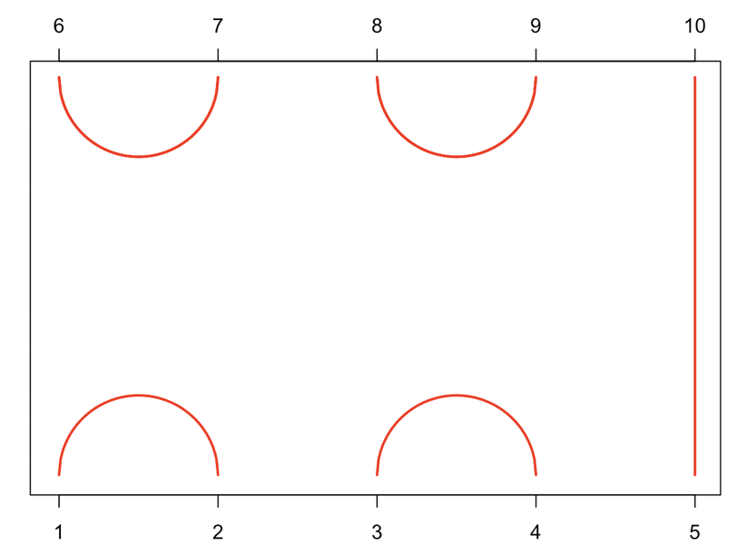
From the start it is clear that if a planar diagram is to have no edge intersections it must be the case that not every node can connect to any other node. Take for example an edgeless PD with nodes on the bottom and on the top, with the bottom nodes labeled through , and the top labeled through (from left to right). While no edges have yet been placed, it remains the case that node is only connectable with nodes . For if it were to connect with node , for example, node would be forced to have its edge intersect with the edge or to remain connectionless, both of which options violate the definition of a PD. Further, node cannot connect with node since that would prevent any other possible top-bottom connections, leaving an odd number of nodes both on top and on bottom, implying at least two nodes which can never be connected. See Figure 2.1.


Thus the set of nodes to which node can connect to even on an edgeless PD is a strict subset of the full node set, containing further a dependence on itself. In particular, let be the connectability of nodes and , with
Then for a given , if is odd, we have if is odd, and if is even then, if and are either both on top or on bottom when is odd, otherwise when is even.
Computer Code 1.
Below are code lines which performs the binary connectablility of any two nodes .
| (2.1) |
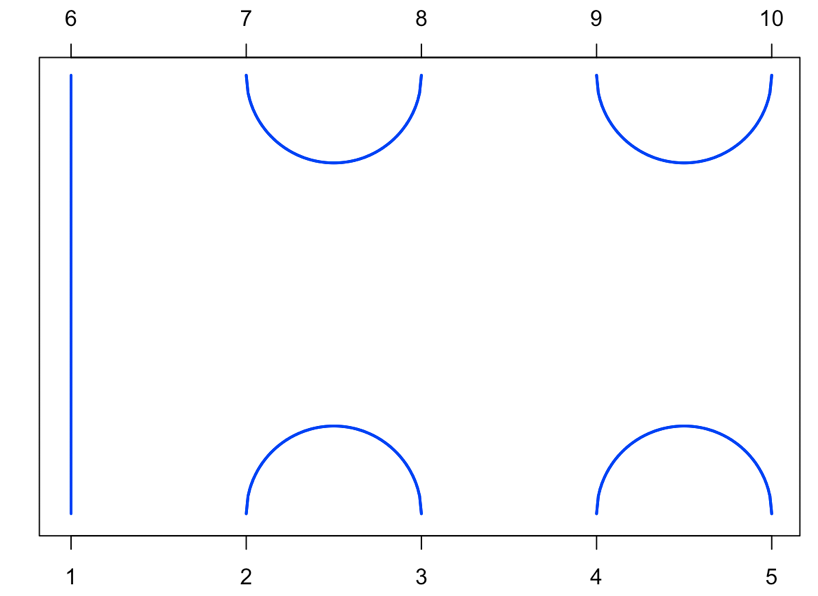
Now that it is clear which nodes can connect to which, even before any edges have been placed (in anticipation of future edge intersections), we turn to considering the particular effects which previously placed edges have on future possibilities. Namely, let be a planer diagram with fixed edges connecting all nodes up to node (not including ) and let be the set of connected nodes. Finally, let be the by matrix associated with , where if node is connected with node (by definition implies either or , and if ). It is clear that node cannot connect to any even if , for they have already been connected by assumption. Further, if node connects to node (which is opposite node on the upper level of the PD), then those nodes which are greater than but less than are also no longer connectable with . Indeed if any of the nodes in connect to node , we would have that is no longer connectable with nodes greater than but less than . We could generalize even further by recognizing that any node will not be connectable with if there is a node in which connects to a node , see Figure 2.2. Lastly we have the edge restrictions which arise from having a node connect with a node with (bottom-bottom connections which surround the node ). Similar to before, these edge placements will make it such that can only connect to nodes which are less than the minimum such and greater than , see Figure 2.2.
Computer Code 2.
Below are code lines which performs the removal of connectablility between node in defined above and .
| (2.2) |
It is worthwhile to note that though in principle we should consider bottom-top connections to the right of node as we did for those to the left of node , if one places edges sequentially (from to ) then future connections need not be considered.


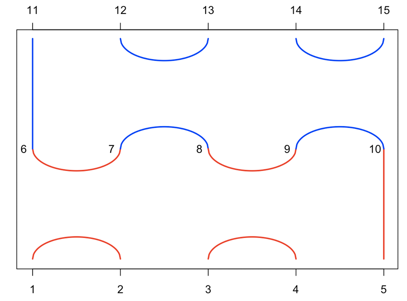
With these restrictions in mind, we can now begin generating all of the possible PDs sequentially. Beginning with node , we have , the set of all possible PDs which have nothing but the first node connected. Form the above discussion it is clear that the cardinality of is (since there are possible nodes to which node can connect). If is one particular PD, then let be all possible planer diagrams which can be generated from by adding only one edge (since the number of next possible edges depends on , so will the cardinality of depend on ). We can now iteratively span the possible PDs via,
with being the complete set of planer diagrams with bottom nodes see Figures 2.3 and 2.4. The code was verified via the equation and by counting the number of PDs obtained for .
Computer Code 3.
Below are code lines which sequentially span the set of possible PDs for dim = N.
| (2.3) |


2.2. The representation of Planer Diagram multiplication
Now that we can both ariticulate planer diagrams using matricies and generate the space for any given dimention, we would like to consider the function which produces the product diagram for any two diagrams. As mentioned in the previus section, the product diagram of two diagrams is the sequential stacking of the second onto the first. In particular, we can consider all pairwise connections in the product diagram:(, , ) and determine whether the pair is connected, given the two input diagrams.
Let be two planer diagrams, with thier respective matrix representations, and let with , its matrix representation. If are a pair of nodes in then if
- (1)
when
- (2)
when
- (3)
If there exists a sequence satisfying
- •
- •
- •
when
- •
In other words, two nodes are connected in the product diagram if there is a path connecting them when the second diagram is placed ontop of the first see Figure 2.5. This can also be verified by evaluating the product series and requiring that .
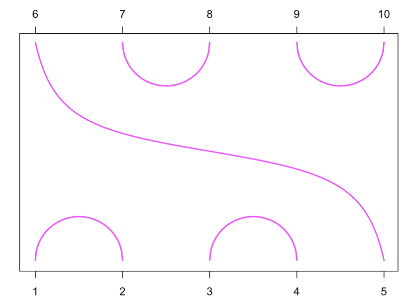
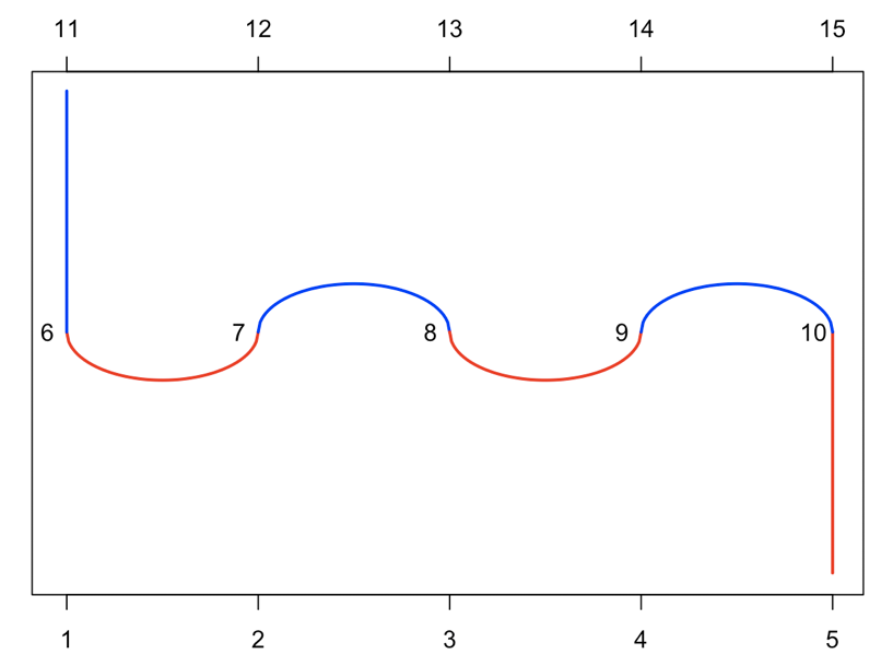
Since the set could in principle contain as many elements as the dimention of the diagram (as was the case in Figure 2.5), determining whether two nodes situated on top and bottom of the product diagram are connected, requires finding all paths of length with . This could be computed by raising to the power see Code 2.4
Computer Code 4.
Below are code lines which solve the product diagram for two diagrams and matrix representions with .
| (2.4) |
3. Computing representations for the generators of planar diagrams
As mentioned, we call the dimensional vector space of planar diagrams . For a given dimension , there are distinct planar diagrams which form a basis of , with generators which are:
| (3.1) |
These generators satisfy the following relations:
| (3.2) |
In this section we will describe a method for finding matrix representations for the generators of , ones which satisfy the relations 3.2. As an example, using the programming language we will find such representations for .
3.1. Representations of the generators for
We begin by creating all possible diagrams in the fourth dimension, which can be seen in Figure 3.1. We have thirteen diagrams in total and we are not including the identity. When the identity is included these diagrams form a basis for and one can verify that is in fact .

Next we create the generators for the fourth dimension, which can be seen in Figure 3.2. As mentioned, these generators satisfy the relations 3.2.

has ideal subspaces such that for any generator and a diagram we have that . One way of finding these ideal subspaces is by looking at the bottoms of the graphs in Figure 3.1 and grouping together all diagrams with the same bottom. We say that two diagrams have the same bottom if their bottom connections, meaning the connections from a bottom node to a bottom node, are the same. In Figure 3.1 this grouping has already been done, with the first eight diagrams belonging to the first ideal and the remaining diagrams belonging to the second ideal. Thus we can split into two subspaces which, as will be shown, can be used to encode the operations of the generators by a matrix.


In Figure 3.3, we show three examples of the multiplication of diagrams and their outcomes. In Figure 3.4, we multiply the first generator with some of the planar diagrams from Figure 3.1 and plot the resulting diagrams. One can verify that each diagram is mapped back into its ideal space. We use this to form a matrix representation of each generator. We form three matrices as follows. Suppose a diagram is mapped to a diagram through multiplication by a generator . If no is obtained by this operation then we place a in the column and row of the matrix . If a is obtained through this operation then we place a in the column and row of the matrix . We place a zero in all other components of . Such a matrix will represent the generator and will satisfy the relations 3.2.
For , we obtain the matrices given in Figure 3.5. Instead of placing a when a bubble is created, we place a in the matrix. From Figure 3.4, we see that the first generator times the second graph in Figure 3.1 is the first graph without a bubble. This is encoded in the first matrix, as a is placed in the second column and first row. The code also verified that the relations 3.2 were satisfied by these three matrices.

References:
References
- [1] C. Kassel, V. Turaev, Braid groups, (Springer, Berlin, 2008).
- [2] L. Kauffman, Knots and physics, (World Sci. Publ., New Jersey, 2001).
- [3] E. Artin, Theory of Braids, Annals of Mathematics 48, 101–126 (1947).
- [4] Z. Wang, Topological Quantum Computation, (AMS, Providence, 2010).