Sifting Through the Static: Moving Object Detection in Difference ImagesKBMOD (Whidden et al. 2019), LSST Science Pipelines (Jurić et al. 2017), astropy (Astropy Collaboration et al. 2013), scikit-image (van der Walt et al. 2014), numpy (Oliphant 2006), CUDA (Nickolls et al. 2008), scikit-learn (Pedregosa et al. 2012), pandas (McKinney 2010), matplotlib (Hunter 2007), tensorflow (Abadi et al. 2016)
Abstract
Trans-Neptunian Objects (TNOs) provide a window into the history of the Solar System, but they can be challenging to observe due to their distance from the Sun and relatively low brightness. Here we report the detection of 75 moving objects that we could not link to any other known objects, the faintest of which has a VR magnitude of using the KBMOD platform. We recover an additional 24 sources with previously-known orbits. We place constraints on the barycentric distance, inclination, and longitude of ascending node of these objects. The unidentified objects have a median barycentric distance of 41.28 au, placing them in the outer Solar System. The observed inclination and magnitude distribution of all detected objects is consistent with previously published KBO distributions. We describe extensions to KBMOD, including a robust percentile-based lightcurve filter, an in-line graphics processing unit (GPU) filter, new coadded stamp generation, and a convolutional neural network (CNN) stamp filter, which allow KBMOD to take advantage of difference images. These enchancements mark a significant improvement in the readiness of KBMOD for deployment on future big data surveys such as LSST.
I Introduction
Small bodies are the final frontier in the study of flux-limited populations in the Solar System. While these objects are primarily very small and often very distant, they are nevertheless critical to our understanding of the formation of the Solar System. For example, Trans-Neptunian Objects (TNOs) contain dynamically-unperturbed relics from the formation of the Solar System (Luu & Jewitt 2002). They provide a window into the early history of the Solar System and enable tests of planetary formation and migration hypotheses. The Nice model (Tsiganis et al. 2005) suggests that all the giant planets formed well-interior to 20 au and migrated outwards due to interactions with planetesimals. Better knowledge of the dynamical populations of TNOs would enable tests of additional and alternative hypotheses regarding the dynamical history of the Solar System, such as the smooth migration of Neptune (Hahn & Malhotra 2005; Nesvorný 2015; Morbidelli & Nesvorný 2020), a stellar flyby (Kenyon & Bromley 2004), or rogue planetary embryos (Gladman & Chan 2006). Improving our understanding of TNO size and orbital distributions, especially at the low-mass end where they are more poorly constrained, will be critical for our understanding of these and other hypotheses.
Well beyond the edge of the Classical Kuiper Belt lies the Oort Cloud. Most famously, the Inner Oort Cloud includes the object Sedna, which is thought to be a member of a larger population of sednoids (Brown et al. 2004). Sedna is an Inner Oort Cloud object with a perihelion of au, but a semimajor axis of au. Therefore, it spends well over of the time on its orbit beyond the detection limit of the survey that discovered it. According to the Minor Planet Center (MPC) database for TNOs, centaurs, and scattered disk objects (SDO), Sedna has the second largest perihelion (after 2012 VP113) of any detected Solar System object. It represents one of the only currently-observable links to the Oort Cloud, a region that contains a wealth of information about the history of the Solar System. If we could increase the number of known sednoids and other Oort Cloud objects, they would provide observational constraints on the formation environment of the Sun (Brasser et al. 2006) and the Sun’s dynamic history in the Milky Way after leaving its formation environment (Kaib et al. 2011).
New and upcoming approaches to survey astronomy provide exciting opportunities for the study of these populations. For example, the upcoming Legacy Survey of Space and Time (Ivezić et al. 2019, LSST; lsst.org;) expects to survey over 18,000 square degrees of the sky 825 times over a period of 10 years, generating about 20 TB of data every 24 hours.
LSST plans to detect Solar System objects from individual images, with a single-visit limiting magnitude in the r band of 24.7, and link these detections to measure orbits. Current projections (LSST Science Collaboration et al. 2009) show that LSST is expected to detect about 40,000 TNOs, which is by itself a large increase over the currently-known 4077 Centaurs, KBOs, and SDOs (MPC). However, if we could coadd the images to increase the signal-to-noise ratio (SNR) of the Solar System detections, then we could recover significantly more objects. Following the formula , coadding just three months of LSST data would increase the limiting magnitude in the band from 24.7 to 26.1. This increase in depth means LSST would detect times more TNOs compared to a single image, assuming the single power-law band KBO distribution of Fraser et al. 2008. Instead of 40,000 TNOs, we could detect TNOs. If we could coadd a year of LSST data, this increases to over 520,000 new TNOs detected (given our simplified assumptions). None of this requires any more data than LSST will already acquire.
Coadding moving objects poses unique challenges compared to coadding stars. Because stars move very slowly compared to most survey cadences, coaddition of a stack of aligned images usually increases the limiting magnitude for stars compared to single images. Solar System objects, however, generally move at on-sky velocities of , due to both the proper motion of the objects and the reflex motion caused by the Earth’s orbit. This means that traditional image coaddition typically does not increase the number of detectable moving objects. Known moving objects may be tracked and aligned along their orbits to improve the quality of the detection, but to use image coaddition to detect new objects with unknown orbits, another approach is required.
The Kernel-Based Moving Object Detection (Whidden et al. 2019, KBMOD;) algorithm takes a time series of images of the same RA and Dec, uses a “track before detect” (TBD) approach to account for the potential motion of objects on an image, and then coadds the shifted images (increasing the SNR of objects with the candidate trajectory). To sample all possible orbital parameters requires searching billions of candidate trajectories even within the footprint of a single charge-coupled device (CCD). Consequently, current implementations of TBD have generally been restricted to narrow-field surveys (Bernstein et al. 2004). KBMOD addresses this by using GPU-accelerated computing to search over a wide range of trajectories for a stack of CCDs in of order 10 minutes.
In this paper, we present a number of algorithmic improvements to KBMOD that allow us to search for moving objects in difference images. We use the Dark Energy Camera (DECam) NEO Data Survey to validate our improvements. This is a larger survey with a longer and more irregular cadence than KBMOD has been applied to in the past. Successfully running on difference images and a more complicated survey shows that KBMOD is beginning to be applicable at the scale needed for upcoming big data surveys like LSST. In Section II, we discuss the DECam NEO Data Survey and the processing we applied to it using the LSST Software Stack. In Section III, we discuss the KBMOD algorithm and present recent improvements. In Section IV, we discuss the results from our analysis, including the detection of unidentified outer Solar System objects. We discuss current limitations and future improvements in Section V.
II Data
II.1 The DECam NEO Survey Data
The DECam NEO Data Survey covered an area on the sky of greater than 2000 square degrees. The 6.7 TB data set from the DECam NEO Data Survey (PI Lori Allen) uses the Dark Energy Camera on the 4m Blanco telescope at the Cerro Tololo Inter-American Observatory (CTIO) (Flaugher et al. 2015). The DECam NEO Data Survey consists of 32 nights of data. In the first 10-night observing run in 2014, Trilling et al. 2017 found 235 unique NEOs.
Each individual image taken by DECam is a composite of 62 2K x 4K science CCDs, with a fill factor of 0.8 (Herner et al. 2020). Each CCD image covers an area of 0.04 square degrees with a pixel scale of 0.27 arcseconds. This results in a total field of view for DECam of about 3 square degrees. The CCDs are thick fully depleted devices, with a peak quantum efficiency above at Å(Flaugher et al. 2015). Gaps between CCDs are between 153 pixels (columns) and 201 pixels (rows). Observations for this data set were taken in the VR filter, a broad optical filter extending from 500 to 760 nm.
We separate this data set into 782 pointing groups based on RA and Dec. CCD 01 and 61 had no data in our images, leading to a set of 60 CCDs per pointing group. We define a pointing group as a set of DECam exposures within of a common RA and Dec and define a pointing as an individual DECam exposure (i.e. a set of 60 CCDs) in a pointing group. Most pointing groups contain between 5 and 25 pointings. Pointing groups characteristically have 5 pointings per night, with all data taken over nearly-consecutive nights. The intra-night pointings are taken about five minutes apart for a total intra-night timespan of approximately 25 minutes.
24 pointing groups had a high stellar number density, with more than 10000 sources detected in a CCD. When astrometrically calibrating these images (see Section II.2), these pointing groups exceeded the memory limits of the available computational resources and were therefore excluded. The current limitations regarding the processing of dense fields with LSST Science Pipelines are described in Sullivan & Bellm 2021. Detectability of moving objects with KBMOD, however, is driven strongly by the quality of the difference images.
372 pointing groups contained data from at least four unique survey nights. Because of the short intra-night image cadence, which can cause slow-moving objects to exhibit minimal motion within a night, we only search over pointing groups with at least four unique survey nights. This ensures that any given KBMOD trajectory will search a sufficiently-large number of unique on-sky positions, thereby reducing the probability of linking of static objects.
In order to comply with computational limitations, we selected 43 pointing groups from the set of 372 pointing groups, focusing our research on higher-quality data. These 43 pointing groups have a total effective search area of approximately 132 square degrees. We refer to these 43 pointing groups as the “search sample”. This down select from 372 pointing groups was as follows. 40 pointing groups existed where all pointings in the pointing group had a maximum seeing full width at half maximum (FWHM) of . These 40 pointing groups make up the bulk of the search sample. There were an additional 12 pointing groups that had over 20 total pointings, but with only 20 pointings with seeing . These pointing groups returned a greater number of erroneous candidate trajectories that required by-eye rejection. This is possibly due to the inclusion of poor-seeing images in the image differencing template (see Section II.2). Due to computational limitations, we elected to run KBMOD on only 3 of these pointing groups, focusing our GPU resources on the 40 pointing groups where all 20 pointings had the required seeing limits. These 3 pointing groups make up the remainder of the search sample.
II.2 Processing the DECam Data
The raw DECam images were processed by the DECam Community Pipeline (Valdes et al. 2014) resulting in a set of InstCal PROCTYPE images, as defined in the NOAO Data Handbook (NOAO 2015). These images are bias and linearity corrected, flat-fielded, and sky-subtracted by the community pipeline. Data quality masks and inverse variance arrays were provided. We downloaded the compressed InstCal data from the NOAO Data Archive between July and November of 2017.
Prior to running the KBMOD pipeline, we first astrometrically calibrate the images in all 782 pointing groups. This was undertaken using the LSST Science Pipelines Software (Jurić et al. 2017). Sources were detected in the individual images. Sources with a were matched to the data from the GAIA Data Release 1 (DR1). The median astrometric scatter for the sources used to fit the CCD world coordinate systems (WCS) was 25 mas; 373 CCDs had an astrometric scatter worse than 100 mas. The median number of sources detected per CCD was 3575.
As a followup to Whidden et al. 2019, we use image differencing to remove non-variable and non-moving sources within an image (as opposed to just masking the sources). We used the LSST Stack to difference the images in the pointing groups using a method based on Alard & Lupton 1998. For the DECam NEO Survey data, we difference each pointing against a coadded template. Given the short intra-night time separation between images of a given pointing group, objects moving slower than of order will not move a full psf width over a single night. We therefore separate a pointing group into two approximately equal groups such that each image in the first group will be separated in time from each image in the second group by at least twelve hours. A coadded template was independently generated from each group and used to difference the opposite group. Because our minimum search velocity is pixels per day ( per day), this guarantees that objects of interest will be much greater than one PSF away from where they were in the coadded template. This means that pointings in the middle of a pointing group—with respect to time — will have the shortest image differencing baseline, and will therefore set a theoretical limit on the slowest-moving objects we can detect.
In order to difference the science images against the coadded template (Alard & Lupton 1998; Zackay & Ofek 2017a; Zackay & Ofek 2017b; Zackay et al. 2016), we need to find a convolution kernel such that for a science image and a coadded template , . Following the approach of Alard & Lupton 1998, we separated the template into local spatial cells of 128x128 pixels. We detected sources in both images, and grouped them into the spatial cells. Stamps of these sources were created with sizes between 21x21 pixels and 35x35 pixels, depending on the FWHM of the source. Stamps in each cell were used to find the local spatially-invariant convolution kernel solutions of each stamp. The local convolutional kernel was modelled as a set of Gaussian functions multiplied with a polynomial. The coefficients of the kernel were then found by solving a least-squares problem. One source (and thus one stamp) was selected for each grid cell based on the clipped mean of all the kernel solutions in the cell. This gave the local convolution kernel for that cell. Chebyshev polynomials of the first kind were fit to the local kernel coefficients in order to determine a model for spatially-variant global convolution kernel coefficients. This global kernel was then used to match the PSF of the coadded template to that of the science image. We matched the template to the science image, rather than the other way around, because the template has less noise and the convolution correlates noise. The two images were then subtracted. Finally, a decorrelation algorithm was run to remove the correlation in the noise of the difference image. After differencing the image, we warp all images in a pointing group to the sky plane of the first pointing in the pointing group. This ensures that a pixel in one pointing will correspond to the same RA and Dec as that of the same pixel in another pointing.
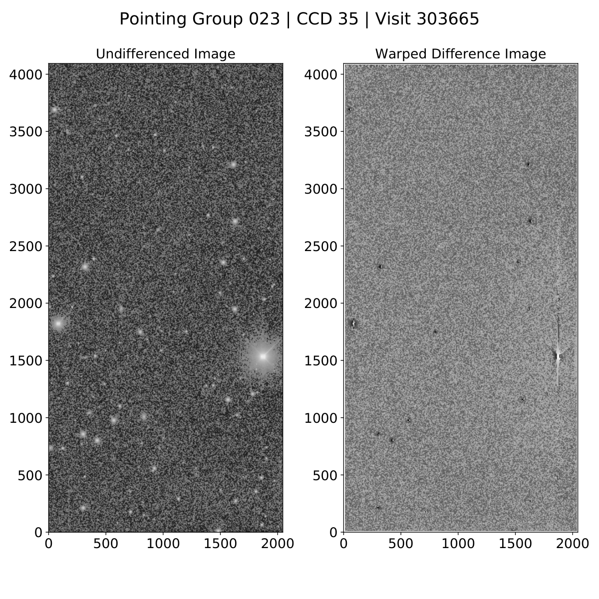
As an example, Figure 1 shows pointing group 023, CCD 35, visit 303665 before and after image differencing and warping. The final image size for the KBMOD image is set by the intersection of the image and the template that is subtracted. Slight misalignments of the pointings in a pointing group may reduce the final image sizes. All pointing groups were, however, aligned to within arcsec in RA and Dec, with all but 28 pointing groups aligned to better than arcsec in both RA and Dec. Therefore the reduction in image area was minimal.
The asteroid search was run for each aligned stack of DECam CCDs independently; we did not search trajectories across CCD boundaries. The effective area on which we are able to search for moving objects is, therefore, about 0.04 square degrees. In other words, a necessary requirement for the detection of a moving object with the KBMOD algorithm is that the object stays within the field of view of an individual CCD for at least two pointings. In practice, we require that an object stay in the field for at least 3 nights (typically 15 pointings). This means that an object must move slower than about to be detected by KBMOD.
III Techniques
KBMOD generates images of likelihood () and variance () from a series of CCD images as described in Whidden et al. 2019. Assuming a Gaussian likelihood function, a stack of and images can then be shifted along a potential asteroid trajectory and summed in order to get the coadded likelihood of a detection ( and ). See Ofek & Zackay 2018 for the optimal approach for source detection with Poisson noise. We define a SNR for a detection such that . In this image, generated for each given angle and velocity vector, any points above some threshold can be considered to be -sigma detections of a moving source. For a single trajectory, we can define the summed likelihood as . The interested reader is directed to Whidden et al. 2019 for more detail.
The large number () of potential asteroid trajectories means that these and images must be searched many times over. For this reason, KBMOD uses massively-parallel GPU computing for the core computations. The current software allows a user to search over potential moving object trajectories in a stack of 10-15 4K x 4K images in under a minute using a consumer-grade GPU (e.g., Nvidia 1080 Ti) (Whidden et al. 2019). Our pointer-arithmetic approach means that we never actually shift and stack images. Rather, we merely sum the previously-calculated likelihoods, utilizing thousands of concurrent GPU threads to keep the computation feasible on consumer-grade hardware.
The DECam NEO data set presents unique filtering challenges compared to Whidden et al. 2019 due to the increased number of potentially-valid trajectories, the short intra-night cadence, and image differencing artifacts. In Whidden et al. 2019, detected sources appearing in the same position in 2 or more images, pixels with counts above 120 counts, and other mask flags set by the DECam community pipeline or the LSST software stack were all masked. In the current data set, we use difference imaging to subtract static sources. This enables us to decrease the masked area of the image, only masking sources flagged as detected if they appear in 10 or more images. However, despite reducing the number of detected individual sources on the image by a factor of about 18 (see Figure 2), leaving most of the image unmasked, coupled with difference imaging artifacts, increases the number of trajectories with by a factor of 10. This problem is worsened by the intranight cadence. The average time between images within a single night is about 5 minutes. This means that for a characteristic trajectory with a velocity of 100 pixels per day, objects will move by less than 1 pixel between images. Conversely, this also means that if a static source appears along the potential trajectory, flux from this object will most likely be present in at least five trajectory data points, introducing repeated outliers into the trajectory.
III.1 Filtering
In order to deal with the increased number of high likelihood trajectories (i.e. with ), we developed faster, more-effective filtering. First, we altered how the GPU and C++ code handed off data to the Python-based filtering, leading to a speed increase of up to 300%. Second, we replaced the Kalman filter used in Whidden et al. 2019 with a more statistically-robust quantile-based filtering method. We describe this new filtering method below.
With a traditional quantile-based filter, the filter rejects data points that are greater than from the central value of the distribution, where is a measure of the spread of the distribution. In the case of a Gaussian distribution, might be estimated by computing the standard deviation of the data and the central value estimated by computing the mean of the data. If we take , then this simple filter would reject any data points that are greater than from the mean.
In the presence of significant outliers, the mean and standard deviation become biased estimators for the central value and the spread of the underlying Gaussian distribution. Following the approach of Ivezić et al. 2014, we adopt a robust estimator for the central value and the true standard deviation of a Gaussian distribution with outliers. Consider the cumulative distribution function (CDF) of a Gaussian distribution
| (1) |
where is the mean, is the standard deviation of the Gaussian, and is the error function. The inverse, then, is given by
| (2) |
By sampling the Gaussian distribution at two quantiles and , we can estimate . To do this, we take the difference of the inverted CDF
| (3) | ||||
| (4) | ||||
| (5) |

Here, C is a coefficient dependent only on the choice of quantiles. and are estimated by selecting values from the lightcurve. The choice of upper and lower quantiles is user-determinable. Here, we estimate using data from the 25th to 75th percentiles, for a coefficient of . Then, we can estimate and from the data by selecting the 25th and 75th percentile values respectively from the data. We can then estimate the standard deviation of the underlying Gaussian distribution with . Given a robust estimator of the spread of the distribution (i.e. ), we apply a filter that rejects any points that are not within (e.g. ) of the median of the data.
We apply this method to the likelihood and/or flux values of each trajectory. We then recompute for the trajectory values that pass the filter and reject the trajectory if the recomputed likelihood () is less than 10. In practice, this filtering method successfully rejects of order erroneous candidate trajectories in approximately s using 30 central processing unit (CPU) cores.
III.2 In-line GPU Filtering
Applying a variant of the filter in the GPU while the search is running, instead of in post-processing, increases the number of potentially-valid trajectories returned to the CPU by KBMOD. In Whidden et al. 2019, KBMOD passed the four trajectories per pixel with the highest from the GPU to the CPU. Other trajectories with the same starting pixel were discarded. Because KBMOD searches of order trajectories for a 2K x 4K image, it is computationally infeasible to keep the results of all evaluated trajectories in GPU RAM. The disadvantage of this approach is that lower-likelihood trajectories may get removed from the search even if they are valid trajectories of true objects. With reduced masking, there are many erroneous candidate trajectories with high likelihood. This means that removing the masks may have increased the probability of discarding valid trajectories.
In-line GPU filtering solves this problem by applying the filtering method to compute before the trajectory is passed back to the CPU. This in-line GPU filter means that if a trajectory has a high only due to an outlier in the data, that trajectory is unlikely to supplant another valid trajectory when GPU results are passed back to the CPU. We also increased the number of returned results per pixel from four to eight. This means that we were able to process about four times as many results per pixel compared to Whidden et al. 2019. The in-line GPU filtering uses a single GPU and is about 10% faster than comparable CPU filtering using 30 CPU cores. Figure 3 demonstrates how the in-line GPU filter returns more potentially-valid trajectories for a given number of trajectories per pixel.
III.3 Median Stamp Coadd Generation
As shown in Figure 1, saturated cores and small image misalignments leave a number of artifacts in the difference image that also have to be accounted for in the filtering process. As in Whidden et al. 2019, we computed the central moments of postage stamps for candidate trajectories. Stamps were rejected if they did not have central moments that were consistent with a Gaussian. In this data, we required that the x, y, xy, xx, and yy moments be strictly less than 0.5, 0.5, 1.5, 36.5, and 36.5 respectively. These values were chosen empirically based on the central moments of known KBOs. We generated coadded stamps by computing the median pixel value for each pixel along the trajectory. This mitigates the effect of image differencing artifacts, improving the performance of the central moment filter.
III.4 CNN Filtering
To further reduce the number of false positives, we filter using a convolutional neural network (CNN). We built a Residual Network with 50 layers (ResNet5011 1 https://github.com/priya-dwivedi/Deep-Learning/blob/master/resnet_keras/Residual_Networks_yourself.ipynb) (He et al. 2016). Residual networks are a type of CNN that add “shortcut connections” into the network architecture, which help to train deeper networks. Training a CNN requires a large amount of representative data. In this case, we needed a large () labeled set of 21x21 stamps containing approximately equal numbers of false positives and true positives. To generate false positives, we ran an untargeted search (with similar grid spacing as described in IV.1) with a coadded likelihood limit of along trajectories unlikely to correspond to real objects (approximately from the direction of the ecliptic). We ran a total of 53 searches with data from 34 unique pointing groups. These pointing groups were not constrained to the search sample. These searches yielded 113,549 21x21 false positive postage stamps. Because KBOs are relatively rare, we could not use real recovered objects to generate the thousands of true positives needed to train the CNN. To circumvent this limitation, we generated 44,950 simulated true positives. To make these stamps, we retrieved 25 21x21 postage stamps from a CCD along a semi-random trajectory. Next, we drew a random brightness from an exponential distribution (with dimmer objects being the most likely). Using this brightness, we added a Gaussian to each background stamp with a random standard deviation ( pixels), a random central offset ( pixels), and a random linear offset ( pixels over the image time baseline). To train the CNN, we cut the false positive stamps and simulated true stamps down to 40,000 randomly-selected coadded stamps each. We used 70% of the data for training, 20% for validation, and the remaining 10% for testing. After 20 epochs, the training set accuracy was about 99%, while the validation set accuracy was about 96%. After training, the test set accuracy was also about 96%.
This CNN returns a predicted probability that a coadded postage stamp contains a simulated object. Because the stamps of simulated objects differ from the stamps of real objects, this probability is not a perfect representation of the likelihood that a coadded stamp contains a real object. However, it creates a user-programmable threshold that can be used to reduce false positives enough that the remaining candidate trajectories can be analyzed by-eye. We reject any stamps with a CNN probability of true less than 75%. As shown in Figure 4, when reviewing only objects with a and using this CNN filter, there are generally fewer than 10 candidate trajectories per CCD that require human by-eye confirmation or rejection.
IV Results
IV.1 Search, Detection, and Recovery
We ran an untargeted KBMOD search on each stack of CCDs in the search sample for a total of 2580 searches. Similar to Whidden et al. 2019, an untargeted search looks for linear trajectories with velocities between 92 and 550 pixels per day ( to ) with angles of from the ecliptic angle. Compared to Whidden et al. 2019, we doubled the resolution of the grid spacing from 256 velocity steps and 128 angle steps to 512 velocity steps and 256 angle steps. This ensured that trajectories would end up separated by no more than about two PSF FWHM from neighboring trajectories.
In order to test the efficiency of these new filtering methods, we generated a list of known objects in the search sample. We used Skybot (Berthier et al. 2006) and JPL Horizons (Giorgini 2015) to find all KBOs that were present in the search sample, with the additional requirement that they be present in the first image of the pointing group. We generated 21x21 pixel postage stamps of the object in each image in which it is present. We developed a variant of KBMOD that computes the likelihoods along a single trajectory then runs the aforementioned quantile-based filtering, and computed the central moments of the postage stamps. Figure 5 shows these results for pointing group 300, CCD 30, object 2015 GQ56. We removed KBOs with an unfiltered . This left us with a “recovery sample” of 26 KBOs.
In the untargeted search of the search sample, we recovered 22 out of 26 (or 84.6%) of the known objects in the recovery sample after all filtering was applied (see Figure 6). The CNN probability threshold was kept at 75%. Recovery statistics for these objects are shown in Figure 7. For object recovery, we discarded any trajectories that had a starting position more than 5 pixels (approximately , or one PSF FWHM) from the predicted location or had a velocity difference from the known velocity of more than 5 pixels per day (approximately ). The median position and speed residuals were and respectively, significantly below the chosen cutoff values. This velocity error corresponds to approximately a 1.27 pixel position error over four days. Using the NOAO DECam Exposure Time Calculator (ETC), we estimate the single-image depth to be at most V. Because the pointing groups contain data from different nights, we computed this limit assuming a new Moon. It is therefore an upper limit. 18 of the recovered objects were fainter than the upper-limit single-image depth. This confirms that KBMOD is able to use difference images to find moving KBOs that are too dim to detect in a single image at the level, extending the result of Whidden et al. 2019 to difference images.
We investigated each of the missed known objects individually. 2013 GY136 (pointing group 204, CCD 57) failed to process due to a CCD that failed image differencing. This reduced the total number of images in CCD 57 to fewer than 20, and CCD 57 was therefore not reprocessed. 2013 GZ137 (pointing group 202, CCD 52) failed CNN filtering with a threshold of 75%, but passes with a threshold of 50%. 2015 GY55 (pointing group 306, CCD 26) starts within 4 pixels of the chip edge, causing this trajectory not to be searched by KBMOD. 2013 GH137 (pointing group 192, CCD 41) has two fully-masked stamps, and two more with partial masking, which may have caused it to be filtered out.
In addition to the detected 22 known objects in the recovery sample, we detected 2 additional known KBOs. These KBOs had an unfiltered along the JPL Horizons trajectories, and were therefore not included in the recovery sample. The best KBMOD trajectories for these objects had a filtered . We then linked these objects back with known KBOs.
IV.2 Orbit Fitting and Analysis
We detected 75 moving objects that we were unable to link to existing objects. Trajectories with that passed all filtering were accepted or rejected with a by-eye examination of the individual stamps, the coadded stamp, and the flux lightcurve.
As shown in Figure 8, we used the method described in Bernstein & Khushalani 2000 to fit barycentric distance , inclination , and longitude of ascending node of both the recovered known objects and the unidentified objects. For the known objects, we compared the orbital parameters fit to the KBMOD trajectory with their respective parameters as reported by JPL Horizons. The medians of the absolute value of the residuals between the best-fit values and the JPL Horizons values are 0.36 au, 0.32 degrees, and 0.92 degrees for , , and respectively. The median values for and of the known objects reported by JPL Horizons are au and respectively. The median values of the unidentified objects for the best-fit and are au and . The three parameters (shown in Figure 8) that are well-fit with our data constrain the plane of the orbit and the initial distance of the object from the Solar System barycenter. Individual values are shown in Table A.
In addition to the method of Bernstein & Khushalani 2000, we used Find_Orb22 2 https://github.com/Bill-Gray/find_orb to fit , , and . This allowed us to compare the best-fit values between the two orbit fitting codes. When best-fit values from Find_Orb were not within 1 of the best-fit value from the Bernstein & Khushalani 2000 code, we show the value as a square in Figure 8. We discarded values with inconsistent inclinations from the remainder of the orbit analysis.
There were a few noteworthy limitations to our dataset and apparent outliers in our best-fit values. Because of the relatively short time baseline of about four days, we were unable to place any meaningful constraints on the other Keplerian elements individually. For three unidentified objects (unidentified object numbers 58, 69, and 74), the orbit fitting code did not return uncertainties. We therefore consider them inconsistent between Bernstein & Khushalani 2000 and Find_Orb. Unidentified object numbers 4, 6, and 8 have a best-fit inclination of . Similarly, known object number 20 (2000 EE173) has a best-fit inclination of , but a JPL Horizons inclination of . However, these 4 objects are all marked as inconsistent between Find_Orb and Bernstein & Khushalani 2000. As such, their best-fit values are removed from further orbital analysis.
To evaluate the consistency of the properties of our detected asteroids with published distributions, we apply the analysis of Whidden et al. 2019 to the detected objects with consistent inclinations reported in this paper. We compared our observed inclination distribution with that of Brown 2001 by using a one-sided Kuiper variant of the Kolmogorov-Smirnov (K-S) test. We use a test statistic of where is the number of objects, and is given by Equation 30 in Whidden et al. 2019.
| (6) |
is the probability for a given inclination distribution that an object has an inclination equal to or below the actual inclination . Some TNO sub-populations have non-uniform inclination distributions around the ecliptic. This is an unmodeled systematic in our test statistic. We compute using Monte Carlo methods. We take inclinations from the Brown 2001 distribution, place them randomly along circular orbits and take all objects within of the ecliptic latitude of discovery. These values allow us to find by calculating the probability that an object with a given has an inclination at or below . We run 1000 Monte Carlo simulations, using the mean as our test statistic. See Section 4.2.1 of Whidden et al. 2019 and Section 3 of Brown 2001 for more detail.
Our mean value for was 1.40. As shown in Figure 9, we reject the null hypothesis that our observed inclinations come from the distribution of Brown 2001 with only 76.6% confidence, which is less than the 1 confidence level of 84.1% (). This is to say that we cannot confidently reject the null hypothesis. We can therefore say that our observed inclinations are consistent with Brown 2001.
We repeated the further comparison of Whidden et al. 2019, using an approximate survey simulation to identify the distribution of objects with a given inclination that we would expect to find given the central RA and Dec of our search sample. We modeled the DECam field of view as a circle with a diameter of . We used the inclinations and orbits from the Monte Carlo simulations used to generate Figure 9 and recorded the objects visible within the simulated camera footprint. We then normalized this simulated object distribution to the number of detected objects in the search sample. Figure 10 shows the simulated distribution (blue) and the observed distribution (orange). The value between the simulated and expected distributions was 8.58, corresponding to a -value of 0.48. We therefore again say that our observed inclinations are consistent with Brown 2001.
IV.3 Magnitude Estimation and Analysis
Figure 11 shows our estimates of the VR magnitude of the known and unidentified objects detected with KBMOD. To fit the VR magnitudes, we generated 25x25 pixel postage stamps in the undifferenced science images following the KBMOD linear trajectory. In each stamp, we fit for the location of the object by maximizing the value of the flux minus the stamp background. The flux was calculated by summing the counts within a circular top-hat psf with a radius of twice the FWHM of the stamp. The local stamp background was estimated from the region outside of this psf. The magnitude zero point was obtained from the InstCal images. We then took the median magnitude value from each set of 15 to 20 magnitude estimates.
As we did in Whidden et al. 2019, we compared our joint magnitude distribution with the apparent magnitude luminosity function presented in Fraser et al. 2008, adjusting for ecliptic latitude by using the inclination distribution of Brown 2001. We use the KBO color reported by Fraser et al. 2008. We note, however, that the DECam VR filter of our observations differs somewhat from the Mosaic2 VR filter used in Fraser et al. 2008. They have similar central wavelengths, but different filter response curves. Individual magnitudes are shown in Table A. The magnitude uncertainties listed in Table A are reported as uncertainties estimated from each set of magnitude estimates.
We approximate the camera footprint as a 3 square degree circle. In practice, our trajectories do not cover the entire camera footprint. Each individual KBMOD search only uses data a single CCD, requiring 60 individual searches to cover a full camera footprint. We further require that each candidate trajectory have at least 15 observations, corresponding to a time baseline of about 3 days. Depending on the search velocity and angle, this means that any objects that start near a CCD edge will not be searched, as the trajectory will go off the CCD edge before the trajectory has the requisite 15 observations. We define an effective search fill factor as the fraction of the CCD that is actually searched with KBMOD. For our search parameters, the search fill factor varies from about 0.5 to about 0.9. Assuming a typical KBO speed and angle of 275 pixels per day with an in-image angle of 4.4 radians gives a typical search fill factor of around 0.7. Multiplying this by the camera active-pixel fill factor of about 0.8 gives a typical net fill factor of approximately 0.55.
Figure 12 shows a histogram of our observed VR magnitudes along with the number expected from Fraser et al. 2008 assuming a fill factor of 1.0 and 0.55. Our joint magnitude distribution is largely inconsistent with Fraser et al. 2008 assuming a fill factor of 1.0, but is consistent to within uncertainties up to about assuming a fill factor of 0.55.
V Discussion
The improvements already presented in this paper helped enable KBMOD to detect 22 out of 26 known objects in the recovery sample. The trajectories of these known objects were recovered with a median error in starting position of less than two pixels. Furthermore, KBMOD was able to detect 75 objects that we were unable to link with any previously-known objects. Although the time baseline of the data was short, we were able to fit the barycentric distance, inclination, and longitude of ascending node of both the known objects and the unidentified objects. The inclination distribution of the recovered objects is consistent with the distribution from Brown 2001. The number of objects detected as a function of magnitude is consistent with the distribution from Fraser et al. 2008 assuming a net fill factor of 0.55.
Whidden et al. 2019 validated KBMOD on the High Cadence Transient Survey (HiTS) (Förster et al. 2016). This work validates algorithmic improvements to KBMOD filtering with a survey that has a time baseline of up to four nights, compared to the three nights used in Whidden et al. 2019. Furthermore, this work validates KBMOD as applied to images that have been differenced with a coadded template.
In so doing, we demonstrated that KBMOD can recover KBOs in difference images from a survey with a longer time baseline and an irregular cadence. However, this required more robust filtering methods. By adding GPU filtering, we have increased the effective number of potentially-valid candidate trajectories that can be passed out of the GPU for further filtering and analysis. With the -based filtering, we have also implemented more robust lightcurve filtering that improves filtering with an irregular image cadence. The CNN ResNet50 stamp filter shows great promise for future stamp filtering methods.
Next-generation astronomy surveys will soon be current-generation. This imminent wealth of data will require new computational tools in order to access its full potential. KBMOD has the potential to increase the number of TNOs detected with LSST from to as well as investigate the faint and mysterious class of objects at the very edge of our Solar System. In terms of probing the sednoids, with three months of coadded data we could detect a Sedna-like object at opposition at over 290 au, as opposed to au for a single image. With a year of coadded data, 290 au increases to 310 au. If we could coadd the entire LSST survey, 310 au increases to over 415 au. Note that objects on elliptical orbits spend much more of their time further from the Sun. If Sedna, which was detected near its perihelion around 90 au (Brown et al. 2004), is representative of a larger population of sedoids, then most of these objects should be closer to apocenter than pericenter. Therefore, a linear increase in detection distance should yield a super-linear increase in the number of detected objects on a similar orbit. With this coaddition approach, it might even be possible to detect inner Oort Cloud objects with perihelion near 400 au, and aphelion well beyond.
Further work is needed before KBMOD will be able to run on LSST. We do not currently address the “look-elsewhere” effect in our search algorithm (Vitells & Gross 2011, e.g.). However, our false positives are already dominated by image artifacts and real sources. Even after filtering, trajectories require human by-eye confirmation or rejection. Because of this requirement of human review, we consider this an acceptable limitation. Future work will further investigate necessary algorithmic improvements to enable machine-only object confirmation, including addressing the “look-elsewhere” effect.
Enabling KBMOD to search across multiple CCDs will increase the effective fill factor, enabling greater completeness and longer time baselines. CCD chip gaps and camera edges will always keep the fill factor below 1.0 (relative to a circular footprint). However, with a CCD chip gap between 153 (columns) and 201 (rows) pixels, a KBO would move past the chip gap and onto the next CCD in about one night, assuming a typical KBO velocity of 275 pixels per day.
Improving image astrometry and image differencing is likely to reduce the number of image differencing artifacts, thereby reducing the number of candidate trajectories requiring by-eye detection. The non-uniformity of the image time baseline in this survey means that artifacts appeared in approximately the same location in up to five images. This posed a unique challenge to filtering out artifacts from candidate trajectories. Because of these factors, and because we ultimately validate each detected object by-eye, we save a full efficiency analysis of KBMOD for a future survey.
Given the relatively low inclination (median value of ) and barycentric distances between 30 au and 50 (median value of au), we find it likely that the majority of the unidentified objects presented in Figure 8 are Kuiper belt objects. However, because the short arcs prevent us from placing accurate constraints on semi-major axis and eccentricity, we are unable to confirm this prediction with the current data. Future follow-up or precovery attempts for these objects may be able to extend the observational arcs enough to accurately constrain them to the Kuiper belt, and perhaps place them within a Kuiper belt subpopulation (e.g. the cold classical Kuiper belt).
The authors acknowledge support from NASA awards NNG16PJ23C and 80NSSC21K1528, and NSF awards AST-1715122, AST-1409547, and OAC-1739419. This work used the Extreme Science and Engineering Discovery Environment (Towns et al. 2014, XSEDE; ), which is supported by National Science Foundation grant number ACI-1548562. This work used the XSEDE Bridges GPU and Bridges-2 GPU-AI at the Pittsburgh Supercomputing Center through allocation TG-AST200009. The authors acknowledge support from the DIRAC Institute in the Department of Astronomy at the University of Washington. The DIRAC Institute is supported through generous gifts from the Charles and Lisa Simonyi Fund for Arts and Sciences, and the Washington Research Foundation.
References
- Abadi et al. (2016) Abadi, M., Barham, P., Chen, J., et al. 2016, in Proceedings of the 12th USENIX Conference on Operating Systems Design and Implementation, OSDI’16 (USA: USENIX Association), 265–283
- Alard & Lupton (1998) Alard, C., & Lupton, R. H. 1998, The Astrophysical Journal, 503, 325. http://stacks.iop.org/0004-637X/503/i=1/a=325
- Astropy Collaboration et al. (2013) Astropy Collaboration, Robitaille, T. P., Tollerud, E. J., et al. 2013, A&A, 558, A33
- Bernstein & Khushalani (2000) Bernstein, G., & Khushalani, B. 2000, The Astronomical journal, 120, 3323
- Bernstein et al. (2004) Bernstein, G. M., Trilling, D. E., Allen, R. L., et al. 2004, The Astronomical Journal, 128, 1364
- Berthier et al. (2006) Berthier, J., Vachier, F., Thuillot, W., et al. 2006, in Astronomical Society of the Pacific Conference Series, Vol. 351, Astronomical Data Analysis Software and Systems XV, ed. C. Gabriel, C. Arviset, D. Ponz, & S. Enrique, 367
- Brasser et al. (2006) Brasser, R., Duncan, M., & Levison, H. 2006, Icarus, 184, 59 . http://www.sciencedirect.com/science/article/pii/S0019103506001230
- Brown (2001) Brown, M. E. 2001, AJ, 121, 2804
- Brown et al. (2004) Brown, M. E., Trujillo, C., & Rabinowitz, D. 2004, The Astrophysical Journal, 617, 645. https://doi.org/10.1086%2F422095
- Flaugher et al. (2015) Flaugher, B., Diehl, H. T., Honscheid, K., et al. 2015, The Astronomical Journal, 150, 150. http://stacks.iop.org/1538-3881/150/i=5/a=150
- Förster et al. (2016) Förster, F., Maureira, J. C., San Martín, J., et al. 2016, ApJ, 832, 155
- Fraser et al. (2008) Fraser, W. C., Kavelaars, J., Holman, M., et al. 2008, Icarus, 195, 827 . http://www.sciencedirect.com/science/article/pii/S0019103508000705
- Giorgini (2015) Giorgini, J. D. 2015, IAU General Assembly, 22, 2256293
- Gladman & Chan (2006) Gladman, B., & Chan, C. 2006, ApJ, 643, L135
- Hahn & Malhotra (2005) Hahn, J. M., & Malhotra, R. 2005, AJ, 130, 2392
- He et al. (2016) He, K., Zhang, X., Ren, S., & Sun, J. 2016, in 2016 IEEE Conference on Computer Vision and Pattern Recognition (CVPR), 770–778
- Herner et al. (2020) Herner, K., Annis, J., Brout, D., et al. 2020, Astronomy and Computing, 33, 100425. https://www.sciencedirect.com/science/article/pii/S2213133720300792
- Hunter (2007) Hunter, J. D. 2007, Computing In Science & Engineering, 9, 90
- Ivezić et al. (2014) Ivezić, Ž., Connolly, A., Vanderplas, J., & Gray, A. 2014, Statistics, Data Mining and Machine Learning in Astronomy (Princeton University Press)
- Ivezić et al. (2019) Ivezić, Ž., Kahn, S. M., Tyson, J. A., et al. 2019, The Astrophysical Journal, 873, 111. https://doi.org/10.3847/1538-4357/ab042c
- Jurić et al. (2017) Jurić, M., Kantor, J., Lim, K. T., et al. 2017, in Astronomical Society of the Pacific Conference Series, Vol. 512, Astronomical Data Analysis Software and Systems XXV, ed. N. P. F. Lorente, K. Shortridge, & R. Wayth, 279
- Kaib et al. (2011) Kaib, N. A., Roškar, R., & Quinn, T. 2011, Icarus, 215, 491 . http://www.sciencedirect.com/science/article/pii/S0019103511003101
- Kenyon & Bromley (2004) Kenyon, S. J., & Bromley, B. C. 2004, Nature, 432, 598
- LSST Science Collaboration et al. (2009) LSST Science Collaboration, Abell, P. A., Allison, J., et al. 2009, LSST Science Book, Version 2.0, LSST Corporation, arXiv:0912.0201
- Luu & Jewitt (2002) Luu, J. X., & Jewitt, D. C. 2002, Annual Review of Astronomy and Astrophysics, 40, 63. https://doi.org/10.1146/annurev.astro.40.060401.093818
- McKinney (2010) McKinney, W. 2010, in Proceedings of the 9th Python in Science Conference, ed. S. van der Walt & J. Millman, 51 – 56
- Morbidelli & Nesvorný (2020) Morbidelli, A., & Nesvorný, D. 2020, in The Trans-Neptunian Solar System, ed. D. Prialnik, M. A. Barucci, & L. A. Young (Elsevier), 25–59. https://www.sciencedirect.com/science/article/pii/B9780128164907000023
- Nesvorný (2015) Nesvorný, D. 2015, The Astronomical journal, 150, 68
- Nickolls et al. (2008) Nickolls, J., Buck, I., Garland, M., & Skadron, K. 2008, Queue, 6, 40. http://doi.acm.org/10.1145/1365490.1365500
- NOAO (2015) NOAO. 2015, NOAO Data Handbook (National Optical Astronomy Observatory). http://ast.noao.edu/sites/default/files/NOAO_DHB_v2.2.pdf
- Ofek & Zackay (2018) Ofek, E. O., & Zackay, B. 2018, AJ, 155, 169
- Oliphant (2006) Oliphant, T. E. 2006, A guide to NumPy (USA: Trelgol Publishing)
- Pedregosa et al. (2012) Pedregosa, F., Varoquaux, G., Gramfort, A., et al. 2012, ArXiv e-prints, arXiv:1201.0490
- Sullivan & Bellm (2021) Sullivan, I., & Bellm, E. 2021, DMTN-171: Fall 2020 status of crowded field processing with the LSST Alert Production Pipelines, LSST Data Management Technical Note DMTN-171, LSST Data Management, doi:10.5281/zenodo.5172677. https://doi.org/10.5281/zenodo.5172677
- Towns et al. (2014) Towns, J., Cockerill, T., Dahan, M., et al. 2014, Computing in Science & Engineering, 16, 62
- Trilling et al. (2017) Trilling, D. E., Valdes, F., Allen, L., et al. 2017, The Astronomical Journal, 154, 170. http://stacks.iop.org/1538-3881/154/i=4/a=170
- Tsiganis et al. (2005) Tsiganis, K., Gomes, R., Morbidelli, A., & Levison, H. F. 2005, Nature, 435, 459, copyright - Copyright Macmillan Journals Ltd. May 26, 2005; Document feature - references; graphs; Last updated - 2017-10-31; CODEN - NATUAS. https://search.proquest.com/docview/204581724?accountid=14784
- Valdes et al. (2014) Valdes, F., Gruendl, R., & DES Project. 2014, in Astronomical Society of the Pacific Conference Series, Vol. 485, Astronomical Data Analysis Software and Systems XXIII, ed. N. Manset & P. Forshay, 379
- van der Walt et al. (2014) van der Walt, S., Schönberger, J. L., Nunez-Iglesias, J., et al. 2014, PeerJ, 2, e453. http://dx.doi.org/10.7717/peerj.453
- Vitells & Gross (2011) Vitells, O., & Gross, E. 2011, Astroparticle Physics, 35, 230
- Whidden et al. (2019) Whidden, P. J., Kalmbach, J. B., Connolly, A. J., et al. 2019, The Astronomical Journal, 157, 119. https://doi.org/10.3847%2F1538-3881%2Faafd2d
- Zackay & Ofek (2017a) Zackay, B., & Ofek, E. O. 2017a, ApJ, 836, 188
- Zackay & Ofek (2017b) —. 2017b, ApJ, 836, 187
- Zackay et al. (2016) Zackay, B., Ofek, E. O., & Gal-Yam, A. 2016, ApJ, 830, 27
Appendix A Table of Detected Object Parameters
| Identifier(pg, ccd) | VR Mag | Barycentric Distance(au) | i (degrees) | (degrees) | Linked toKnown Object |
|---|---|---|---|---|---|
| (190,20) | 24.460.22 | 38.382.42 | 8.582.99 | 48.734.99 | True |
| (190,23) | 24.130.82 | 42.022.43 | 3.100.50 | 84.3510.33 | True |
| (191,27) | 24.270.23 | 39.762.41 | 3.601.33 | 36.210.22 | True |
| (191,47) | 24.180.40 | 31.872.31 | 4.341.69 | 31.891.58 | True |
| (192,06) | 24.510.27 | 54.002.60 | 2.520.92 | 206.204.28 | True |
| (192,36) | 24.480.40 | 41.972.46 | 5.161.89 | 35.820.84 | True |
| (192,42) | 24.370.29 | 43.622.47 | 2.140.78 | 24.315.10 | True |
| (193,05) | 24.610.29 | 39.752.41 | 2.750.35 | 90.869.91 | True |
| (193,18) | 24.440.37 | 42.302.51 | 11.274.05 | 206.484.19 | True |
| (193,21) | 24.480.36 | 46.192.49 | 2.900.67 | 73.629.82 | True |
| (193,23) | 23.720.19 | 43.082.46 | 2.820.59 | 173.4211.60 | True |
| (193,50) | 24.310.29 | 32.362.51 | 17.957.29 | 42.201.84 | True |
| (301,46) | 23.760.57 | 44.952.61 | 2.020.74 | 8.435.74 | True |
| (302,06) | 22.830.29 | 38.443.69 | 30.5517.70 | 199.082.98 | True |
| (195,47) | 22.970.15 | 32.482.45 | 9.903.56 | 14.358.85 | True |
| (202,48) | 23.260.17 | 40.882.58 | 16.225.92 | 47.863.56 | True |
| (203,09) | 24.180.68 | 44.532.48 | 2.080.36 | 166.5112.63 | True |
| (203,11) | 23.920.20 | 48.252.90 | 24.399.49 | 215.161.73 | True |
| (203,43) | 24.520.47 | 44.812.53 | 8.683.05 | 45.782.30 | True |
| (205,18) | 24.040.59 | 41.572.47 | 3.220.04 | 122.654.57 | True |
| (284,29) | 22.060.46 | 34.992.54 | 173.360.54 | 136.6510.42 | True |
| (285,22) | 20.750.07 | 41.603.94 | 14.006.38 | 349.3217.52 | True |
| (296,28) | 22.690.16 | 41.222.71 | 6.751.43 | 252.0813.39 | True |
| (300,30) | 23.700.98 | 46.902.94 | 17.797.56 | 24.730.84 | True |
| (017,46) | 23.990.33 | 35.592.45 | 5.310.24 | 285.017.11 | False |
| (018,20) | 23.931.26 | 38.642.45 | 4.920.10 | 316.135.57 | False |
| (018,52) | 24.780.80 | 46.172.57 | 12.083.39 | 243.098.42 | False |
| (191,19) | 24.990.58 | 42.912.44 | 1.580.62 | 39.441.65 | False |
| (191,50) | 24.140.36 | 30.671.17 | 156.064.63 | 216.930.01 | False |
| (192,05) | 24.410.24 | 41.542.43 | 1.070.49 | 58.6910.24 | False |
| (192,08) | 24.200.23 | 30.661.17 | 155.994.65 | 216.930.01 | False |
| (192,08) | 24.740.24 | 40.492.42 | 0.800.37 | 42.482.53 | False |
| (192,54) | 22.240.04 | 32.951.16 | 166.542.55 | 41.030.58 | False |
| (193,07) | 24.420.33 | 41.652.44 | 3.000.38 | 91.139.69 | False |
| (193,10) | 24.650.52 | 42.192.44 | 2.700.37 | 89.6410.07 | False |
| (193,14) | 23.960.41 | 42.472.45 | 4.011.17 | 62.147.95 | False |
| (193,14) | 25.020.93 | 41.862.43 | 1.830.10 | 107.819.23 | False |
| (193,26) | 23.970.14 | 42.552.44 | 3.060.93 | 63.128.68 | False |
| (193,32) | 24.480.64 | 36.702.37 | 4.861.69 | 50.565.10 | False |
| (193,40) | 24.620.31 | 42.112.44 | 2.220.62 | 66.859.23 | False |
| (301,30) | 22.651.01 | 41.402.73 | 16.186.70 | 203.610.50 | False |
| (301,40) | 23.690.40 | 41.282.65 | 0.630.24 | 238.2515.08 | False |
| (305,14) | 23.270.34 | 39.362.42 | 7.042.54 | 36.553.74 | False |
| (305,28) | 23.400.43 | 41.712.44 | 1.240.04 | 129.488.93 | False |
| (305,60) | 23.230.46 | 33.712.69 | 24.3310.40 | 206.560.24 | False |
| (306,47) | 23.420.28 | 42.582.51 | 4.020.99 | 63.8510.83 | False |
| (306,48) | 22.900.54 | 38.662.59 | 13.045.12 | 37.814.62 | False |
| (306,49) | 22.930.69 | 38.262.46 | 2.750.07 | 130.355.44 | False |
| (307,05) | 23.360.69 | 32.652.60 | 5.200.24 | 135.877.47 | False |
| (310,29) | 22.950.18 | 46.002.53 | 4.400.11 | 105.055.51 | False |
| (310,29) | 23.010.55 | 47.062.54 | 4.180.03 | 125.853.95 | False |
| (310,36) | 23.930.68 | 39.593.05 | 28.7012.84 | 202.303.92 | False |
| (311,46) | 22.380.19 | 41.202.90 | 25.1210.68 | 23.800.88 | False |
| (313,60) | 22.850.24 | 34.452.43 | 5.221.24 | 248.7111.50 | False |
| (314,13) | 23.210.26 | 34.062.38 | 4.651.81 | 213.632.65 | False |
| (316,45) | 23.170.51 | 45.232.49 | 6.532.19 | 14.694.92 | False |
| (316,55) | 23.060.22 | 42.892.46 | 6.752.36 | 19.173.99 | False |
| (194,18) | 24.610.68 | 43.062.45 | 1.510.34 | 351.7313.15 | False |
| (194,21) | 24.420.26 | 43.552.46 | 2.940.83 | 5.449.74 | False |
| (194,27) | 24.52… | 34.992.46 | 14.265.49 | 222.732.60 | False |
| (195,20) | 24.140.21 | 48.322.78 | 21.317.74 | 225.493.55 | False |
| (195,60) | 24.840.70 | 34.812.41 | 4.340.03 | 311.054.15 | False |
| (196,30) | 24.610.57 | 35.512.58 | 14.996.01 | 25.815.82 | False |
| (197,19) | 24.460.49 | 43.062.46 | 2.460.34 | 341.7011.82 | False |
| (197,34) | 22.840.23 | 38.202.45 | 10.773.82 | 229.644.24 | False |
| (197,36) | 24.750.73 | 41.912.45 | 3.260.80 | 359.8211.28 | False |
| (197,58) | 24.130.60 | 35.472.71 | 23.389.82 | 32.452.94 | False |
| (202,05) | 23.880.13 | 41.772.45 | 3.540.03 | 121.934.22 | False |
| (202,20) | 23.600.40 | 46.022.53 | 8.612.62 | 58.426.64 | False |
| (202,27) | 23.440.28 | 39.072.44 | 8.622.75 | 57.976.73 | False |
| (202,36) | 23.710.29 | 38.383.22 | 34.1815.74 | 42.952.59 | False |
| (202,40) | 23.430.24 | 34.433.42 | 35.9918.64 | 41.402.35 | False |
| (202,42) | 24.270.60 | 42.864.42 | 46.1626.51 | 41.312.46 | False |
| (203,12) | 24.180.56 | 45.412.56 | 10.713.84 | 209.743.52 | False |
| (203,43) | 24.571.29 | 41.762.45 | 1.040.01 | 130.9014.38 | False |
| (204,21) | 23.951.04 | 46.442.54 | 5.712.04 | 211.763.18 | False |
| (204,21) | 24.040.45 | 42.462.48 | 2.510.78 | 62.477.19 | False |
| (204,27) | 24.000.42 | 47.182.59 | 10.793.91 | 216.791.34 | False |
| (204,41) | 24.070.48 | 44.492.50 | 0.610.24 | 177.4321.56 | False |
| (205,22) | 24.370.45 | 38.392.49 | 7.672.68 | 198.457.99 | False |
| (205,23) | 24.140.33 | 41.252.53 | 11.444.13 | 205.705.58 | False |
| (205,49) | 24.260.40 | 43.632.49 | 2.330.06 | 139.218.76 | False |
| (284,13) | 23.450.18 | 36.40… | 31.17… | 10.41… | False |
| (284,29) | 23.590.68 | 37.564.53 | 9.234.19 | 340.7722.78 | False |
| (284,42) | 22.600.18 | 41.543.52 | 10.564.43 | 238.9918.72 | False |
| (284,52) | 23.680.27 | 41.113.67 | 10.453.41 | 340.2316.58 | False |
| (284,59) | 23.250.62 | 36.704.97 | 8.473.74 | 254.1932.60 | False |
| (288,15) | 23.890.48 | 45.703.47 | 17.819.31 | 12.574.05 | False |
| (288,29) | 23.410.28 | 44.984.41 | 30.2020.59 | 204.553.45 | False |
| (288,48) | 23.540.27 | 40.103.98 | 19.5513.47 | 208.926.35 | False |
| (289,48) | 23.510.41 | 38.026.91 | 21.0227.89 | 213.7218.67 | False |
| (289,48) | 23.820.51 | 42.453.30 | 8.963.85 | 233.2415.66 | False |
| (290,23) | 23.840.37 | 47.453.38 | 26.3512.60 | 211.834.95 | False |
| (291,08) | 23.250.26 | 34.80… | 40.90… | 18.00… | False |
| (291,27) | 23.850.61 | 33.1010.91 | 29.4564.35 | 206.9713.80 | False |
| (296,43) | 23.600.31 | 38.912.78 | 6.000.71 | 327.1010.71 | False |
| (297,46) | 23.330.27 | 33.724.03 | 7.330.07 | 291.616.21 | False |
| (298,22) | 23.950.41 | 45.594.09 | 36.7320.72 | 216.217.06 | False |
| (298,26) | 22.380.59 | 33.54… | 39.53… | 17.32… | False |