跳到论文正文
W Papers独立论文阅读器 arXiv:2109.03110 论文正文 计算阅读时间 · 0%
引用这篇论文根据当前论文元数据生成,正式投稿前建议核对。


License: CC BY 4.0
arXiv:2109.03110v1 [math.OC] 07 Sep 2021
\NatBibNumeric
\MSCCLASS

90C26, 90C46, 90C30

Local Optimality Conditions for a Class of Hidden Convex Optimization

Mengmeng Song1    Yong Xia1    Hongying Liu1    Corresponding Author
Abstract

Hidden convex optimization is such a class of nonconvex optimization problems that can be globally solved in polynomial time via equivalent convex programming reformulations. In this paper, we focus on checking local optimality in hidden convex optimization. We first introduce a class of hidden convex optimization problems by jointing the classical nonconvex trust-region subproblem (TRS) with convex optimization (CO), and then present a comprehensive study on local optimality conditions. In order to guarantee the existence of a necessary and sufficient condition for local optimality, we need more restrictive assumptions. To our surprise, while (TRS) has at most one local non-global minimizer and (CO) has no local non-global minimizer, their joint problem could have more than one local non-global minimizer.

keywords
Optimality condition, Hidden convexity, Local optimality, Trust region subproblem
††runningauthor: M. Song et al.††runningtitle: Local Optimality for Hidden Convex Optimization††authors: songmengmeng@buaa.edu.cn, yxia@buaa.edu.cn, liuhongying@buaa.edu.cn,
11, School of Mathematical Sciences, Beihang University, Beijing, 100191, People’s Republic of China,
††affiliation: ††affiliation: ††affiliation: ††affiliation:

1 Introduction

As a fundamental topic in operations research, convex optimization has a rapid development in the last two decades [2, 18], thanks to its popular applications in machine learning [3]. One of the key to the algorithmic success in convex optimization is that any local minimizer is in fact a global one. The situation is different in nonconvex optimization, which is in general NP-hard, and often has many local non-global minimizers. Local optimal solutions play a great role in globally solving structured nonconvex optimization problem [1]. However, as shown in [17, 20], checking local optimality of a nonconvex quadratic program is already NP-hard. That is, local optimization is as difficult as global optimization. On the other hand, we notice that not all nonconvex optimization problems are difficult to globally solve. For example, hidden convex optimization admits an equivalent polynomial-solvable convex programming reformulation, see [25] for a recent survey. Accordingly, we ask

Question 1.1

Can we go far beyond the standard local optimality conditions for hidden convex optimization?

A typical hidden convex optimization is the following trust region subproblem (TRS):

minx∈ℝn⁡{12​xT​H​x+cT​x:xT​x≤Δ},\begin{array}[]{cl}\min\limits_{x\in{\mathbb{R}}^{n}}\{\tfrac{1}{2}x^{T}Hx+c^{T}x:x^{T}x\leq\Delta\},\end{array} (TRS)

where H=HT∈ℝn×n,c∈ℝnH=H^{T}\in{\mathbb{R}}^{n\times n},c\in{\mathbb{R}}^{n} and Δ>0\Delta>0. (TRS) plays a key role in trust region methods for solving nonlinear programming problems [5, 28]. In the early 1980s, Gay [9], Sorensen [21], Moré and Sorensen [16] have established necessary and sufficient optimality condition for the global minimizer of (TRS). Observing this, Ye [27] showed that (TRS) can be globally solved in polynomial time. In 1994, Martínez [15] proved that (TRS) has at most one local non-global minimizer, and then established a necessary optimality condition and a sufficient one for the local non-global minimizer of (TRS). Observing the gap between necessary and sufficient conditions, Tao and An [22] pointed out that “For the trust-region subproblem, it is interesting to note the following paradox: checking a global solution is easier than checking a local nonglobal one.” It seems that the answer to Question 1.1 is negative on (TRS). In 2020, Wang and Xia [23] broke Tao and An’s paradox by proving that Martínez’s sufficient optimality condition [15] for (TRS) is also necessary. In the same paper, it is also shown that the local non-global minimizer can be found or proved to do not exist in polynomial time. Thus, Wang and Xia’s result gives a positive answer to Question 1.1 on (TRS).

Towards answering Question 1.1, we introduce in this paper a class of nonconvex optimization, which joints nonconvex trust-region subproblem with convex optimization:

minx∈ℝn,y∈ℝm12​xT​H​x+cT​x+f0​(y)s.t.xT​x+f1​(y)≤0fj(y)≤0,j=2,⋯,k,\begin{array}[]{cl}\min\limits_{x\in{\mathbb{R}}^{n},y\in{\mathbb{R}}^{m}}&\tfrac{1}{2}x^{T}Hx+c^{T}x+f_{0}(y)\\ {\rm s.t.}&x^{T}x+f_{1}(y)\leq 0\\ &\ \ \ \ \ \ \ \ \,f_{j}(y)\leq 0,j=2,\cdots,k,\end{array} (TRS-C)

where H=HT∈ℝn×n,c∈ℝn,k∈ℤ+H=H^{T}\in{\mathbb{R}}^{n\times n},c\in{\mathbb{R}}^{n},k\in\mathbb{Z}^{+}, and fj​(⋅)​(j=0,1,⋯,k)f_{j}(\cdot)~(j=0,1,\cdots,k) are convex and twice continuously differentiable. Throughout this paper, we assume H⋡0H\nsucceq 0, otherwise (TRS-C) is a convex optimization problem. In particular, setting m=1,k=1,f0≡0,f1≡−Δm=1,k=1,f_{0}\equiv 0,f_{1}\equiv-\Delta, (TRS-C) reduces to (TRS).

As we have mentioned above, (TRS) has at most one local non-global minimizer, and convex optimization problem has no local non-global minimizer. Notice that (TRS-C) joints (TRS) with convex optimization. So, it is natural to expect a positive answer to the following question:

Question 1.2

Does (TRS-C) have at most one local non-global minimizer?

We may consider another special case of (TRS-C) by setting m=1,k=1,f0​(y)=σp​yp2,f1​(y)=−ym=1,k=1,f_{0}(y)=\tfrac{\sigma}{p}y^{\tfrac{p}{2}},f_{1}(y)=-y, where σ>0\sigma>0 and p>2p>2 are two parameters:

minx∈ℝn,y∈ℝ⁡{12​xT​H​x+cT​x+σp​yp2:xT​x−y≤0}.\min\limits_{x\in{\mathbb{R}}^{n},y\in{\mathbb{R}}}\{\tfrac{1}{2}x^{T}Hx+c^{T}x+\tfrac{\sigma}{p}y^{\tfrac{p}{2}}:x^{T}x-y\leq 0\}. (1)

The univariate variable yy can be removed by substituting the constraint into the objection. Then (1) is equivalent to the following unconstrained optimization

minx∈ℝn⁡12​xT​H​x+cT​x+σp​‖x‖p,\min\limits_{x\in{\mathbb{R}}^{n}}\tfrac{1}{2}x^{T}Hx+c^{T}x+\tfrac{\sigma}{p}\|x\|^{p}, (pp-RS)

which is known as p−p-regularized subproblem [11]. In particular, the cubic regularization (p=3p=3) was first introduced in [12] and then widely applied in nonlinear programming, see for example, [4, 19, 24]. The other special case of ( p -RS) with p=4p=4 corresponds to the double-well potential optimization [6, 26]. Recently, Hsia et al. [13] established necessary and sufficient optimality conditions for both global and local minimizers of ( p -RS) with any p>2p>2. In the same paper, ( p -RS) is shown to have at most one local non-global minimizer. Thus, both Question 1.1 and 1.2 have positive answers on ( p -RS).

In this paper, we give a comprehensive study on (TRS-C). We first reveal its hidden convexity by establishing necessary and sufficient optimality condition for global minimizer. It makes sense as (TRS-C) joints a hidden convex with a convex optimization problem. We then establish necessary and sufficient optimality conditions for local non-global minimizer, respectively. However, the gap of two conditions exists for the general case. In order to close this gap, we need more assumptions. It supports the conjecture that Question 1.1 has no positive answer. For Question 1.2, to our surprise, the answer is negative. Actually, (TRS-C) may have a finite number of local non-global minimizers. Only for very special cases including (TRS) and ( p -RS), (TRS-C) has at most one local non-global minimizer. Consequently, we conclude that the existence of many local minimizers is NOT a (or at least not a unique) reason making global optimization difficult.

The remainder of this paper is organized as follows. Section 2 presents necessary and sufficient conditions for global minimizers of (TRS-C). Section 3 establishes necessary and sufficient conditions for local non-global minimizer of (TRS-C), respectively. These conditions are further characterized by a scalar function for a special case of (TRS-C) with k=1k=1 in Section 4. We consider another special case of (TRS-C) where f1​(y)f_{1}(y) is a linear function in Section 5. Two instances with more than one local non-global minimizer are constructed. Then a sufficient condition is presented to guarantee that (TRS-C) has at most one local non-global minimizer. As an extension of (TRS) and ( p -RS), we identify a class of cases of (TRS-C) where local non-global minimizer enjoys a necessary and sufficient optimality condition. We conclude the paper in the last section with a few open questions.

Notations. For any matrix P∈ℝn×nP\in{\mathbb{R}}^{n\times n}, PTP^{T} and det(P)\det{(P)} denote the transposition and determination of PP, respectively. P≻(⪰)​0P\succ(\succeq)0 denotes that PP is positive (semi)definite. Let II stand for the identity matrix of order nn. For a vector x∈ℝnx\in{\mathbb{R}}^{n}, Diag⁡(x){\rm Diag}(x) returns a diagonal matrix with diagonal elements being x1,⋯,xnx_{1},\cdots,x_{n}. Let f−1​(⋅)f^{-1}(\cdot) represent the inverse of function f⁡(⋅)f(\cdot), if it exists. ℤ+\mathbb{Z}^{+} denotes the set of all positive integers. The eigenvalue decomposition of the symmetric matrix HH is given by

H=V​Diag​(λ1,⋯,λn)​VT,H=V{\rm Diag}(\lambda_{1},\cdots,\lambda_{n})V^{T}, (2)

where V=(v1,v2,⋯,vn)∈ℝn×nV=(v_{1},v_{2},\cdots,v_{n})\in{\mathbb{R}}^{n\times n} is orthogonal, and λi\lambda_{i} is the ii-th smallest eigenvalue of HH.

2 Global Optimality Condition

In this section, we present the necessary and sufficient optimality condition for the global minimizer of (TRS-C), where the Slater condition is assumed.

Theorem 2.1

Assume that (x∗,y∗)∈ℝn×ℝm(x_{*},y_{*})\in{\mathbb{R}}^{n}\times{\mathbb{R}}^{m} is a global minimizer of (TRS-C) and there exists y¯\bar{y} such that fj(y¯)<0,j=1,⋯,kf_{j}(\bar{y})<0,~j=1,\cdots,k. There exist μj∗≥0\mu^{*}_{j}\geq 0 (j=1,⋯,kj=1,\cdots,k) such that

(H+μ1∗​I)​x∗+c=0,\displaystyle(H+\mu^{*}_{1}I)x_{*}+c=0, (3)
∇f0(y∗)+μ1∗2∇f1(y∗)+∑j=2kμj∗∇fj(y∗)=0,\displaystyle\nabla f_{0}(y_{*})+\frac{\mu^{*}_{1}}{2}\nabla f_{1}(y_{*})+\sum_{j=2}^{k}\mu^{*}_{j}\nabla f_{j}(y_{*})=0, (4)
x∗Tx∗+f1(y∗)=0,μj∗fj(y∗)=0,j=2,⋯,k,\displaystyle x_{*}^{T}x_{*}+f_{1}(y_{*})=0,\ \ \mu^{*}_{j}f_{j}(y_{*})=0,~j=2,\cdots,k, (5)
H+μ1∗​I⪰0.\displaystyle H+\mu^{*}_{1}I\succeq 0. (6)

Proof. Note that λ1<0\lambda_{1}<0 for H⋡0H\nsucceq 0. Since (x∗,y∗)(x_{*},y_{*}) is a global minimizer of (TRS-C), then x∗x_{*} solves

minx∈ℝn⁡{12​xT​H​x+cT​x:xT​x≤−f1​(y∗)}.\min_{x\in{\mathbb{R}}^{n}}\{\tfrac{1}{2}x^{T}Hx+c^{T}x:~x^{T}x\leq-f_{1}(y_{*})\}. (7)

We conclude that

x∗T​x∗+f1​(y∗)=0.x_{*}^{T}x_{*}+f_{1}(y_{*})=0. (8)

Otherwise, it follows from x∗T​x∗+f1​(y∗)<0x_{*}^{T}x_{*}+f_{1}(y_{*})<0 that HH is positive semidefinite by second order necessary optimality, which contradicts the fact λ1<0\lambda_{1}<0.

Therefore, (x∗,y∗)(x_{*},y_{*}) remains a global minimizer of

minx∈ℝn,y∈ℝmF⁡(x,y):=12​xT​H​x+cT​x+f0​(y)−λ12​(xT​x+f1​(y))s.t.xT​x+f1​(y)=0fj(y)≤0,j=2,⋯,k.\begin{array}[]{cl}\min\limits_{x\in{\mathbb{R}}^{n},y\in{\mathbb{R}}^{m}}&F(x,y):=\tfrac{1}{2}x^{T}Hx+c^{T}x+f_{0}(y)-\frac{\lambda_{1}}{2}(x^{T}x+f_{1}(y))\\ {\rm s.t.}&x^{T}x+f_{1}(y)=0\\ &\ \ \ \ \ \ \ \,\ f_{j}(y)\leq 0,~j=2,\cdots,k.\end{array}

Now, consider a convex optimization relaxation of the above problem:

minx∈ℝn,y∈ℝmF⁡(x,y)=12​xT​(H−λ1​I)​x+cT​x+f0​(y)−λ12​f1​(y)s.t.xT​x+f1​(y)≤0fj(y)≤0,j=2,⋯,k.\begin{array}[]{cl}\min\limits_{x\in{\mathbb{R}}^{n},y\in{\mathbb{R}}^{m}}&F(x,y)=\tfrac{1}{2}x^{T}(H-\lambda_{1}I)x+c^{T}x+f_{0}(y)-\frac{\lambda_{1}}{2}f_{1}(y)\\ {\rm s.t.}&x^{T}x+f_{1}(y)\leq 0\\ &\ \ \ \ \ \ \ \ \,f_{j}(y)\leq 0,j=2,\cdots,k.\end{array} (9)

Let (x,y)(x,y) be any feasible solution to (9) with xT​x+f1​(y)<0x^{T}x+f_{1}(y)<0. Let v1v_{1} be an eigenvector of HH corresponding to λ1\lambda_{1} (i.e., H​v1=λ1​v1Hv_{1}=\lambda_{1}v_{1}) and satisfy cT​v1≤0c^{T}v_{1}\leq 0. Then there is a τ>0\tau>0 such that x¯=x+τ​v1\bar{x}=x+\tau v_{1} satisfies x¯T​x¯+f2​(y)=0\bar{x}^{T}\bar{x}+f_{2}(y)=0. We can verify that (x¯,y)(\bar{x},y) is feasible to (9), and

12​x¯T​(H−λ1​I)​x¯+cT​x¯\displaystyle\frac{1}{2}{\bar{x}}^{T}(H-\lambda_{1}I)\bar{x}+c^{T}\bar{x} =\displaystyle= 12​xT​(H−λ1​I)​x+cT​x+τ​cT​v1\displaystyle\frac{1}{2}x^{T}(H-\lambda_{1}I)x+c^{T}x+\tau c^{T}v_{1}
≤\displaystyle\leq 12​xT​(H−λ1​I)​x+cT​x.\displaystyle\frac{1}{2}x^{T}(H-\lambda_{1}I)x+c^{T}x.

Therefore, F⁡(x¯,y)≤F⁡(x,y)F(\bar{x},y)\leq F(x,y). It follows that (x∗,y∗)(x_{*},y_{*}) must be a global minimizer of (9). Notice that (9) is a convex optimization problem where Slater condition holds by assumption. According to the first order necessary optimality condition, there exist μ¯1≥0\bar{\mu}_{1}\geq 0 and μ∗j≥0,j=2,⋯,k\mu^{*}_{j}\geq 0,j=2,\cdots,k, which satisfy

(H+μ¯1I−λ1I)x∗=−c,∇f0(y∗)+μ¯1−λ12∇f1(y∗)+∑j=2kμj∗∇fj(y∗)=0,\displaystyle(H+\bar{\mu}_{1}I-\lambda_{1}I)x_{*}=-c,\ \ \nabla f_{0}(y_{*})+\frac{\bar{\mu}_{1}-\lambda_{1}}{2}\nabla f_{1}(y_{*})+\sum_{j=2}^{k}\mu^{*}_{j}\nabla f_{j}(y_{*})=0, (10)
μ¯1(x∗Tx∗+f1(y∗))=0,μj∗fj(y∗)=0,j=2,⋯,k.\displaystyle\bar{\mu}_{1}(x_{*}^{T}x_{*}+f_{1}(y_{*}))=0,\ \ \mu^{*}_{j}f_{j}(y_{*})=0,j=2,\cdots,k. (11)

Define μ1∗=μ¯1−λ1\mu^{*}_{1}=\bar{\mu}_{1}-\lambda_{1}. Equations (8), (10) and (11) imply that μj∗,j=1,⋯,k\mu^{*}_{j},j=1,\cdots,k, satisfy (3), (4) and (5). Since H−λ1​I⪰0H-\lambda_{1}I\succeq 0 and μ¯1≥0\bar{\mu}_{1}\geq 0, we have H+μ1∗​I⪰0H+\mu^{*}_{1}I\succeq 0, i.e., (6) holds true.   

Remark 2.2

(TRS-C) admits an equivalent convex reformulation (9), which reveals the hidden convexity of (TRS-C).

Theorem 2.1 establishes a necessary condition for global optimality of (x∗,y∗)(x_{*},y_{*}). The next result shows that it is also a sufficient condition.

Theorem 2.3

Let (x∗,y∗)∈ℝn×ℝm(x_{*},y_{*})\in{\mathbb{R}}^{n}\times{\mathbb{R}}^{m} be a feasible solution to (TRS-C). If there exist μ∗j≥0,j=1,⋯,k\mu^{*}_{j}\geq 0,j=1,\cdots,k, satisfying (3)-(6). Then (x∗,y∗)(x_{*},y_{*}) is a global minimizer of (TRS-C).

Proof. Define μ¯1=μ1∗+λ1\bar{\mu}_{1}=\mu^{*}_{1}+\lambda_{1}. It follows from H+μ1∗​I⪰0H+\mu^{*}_{1}I\succeq 0 that μ¯1≥0\bar{\mu}_{1}\geq 0. Substituting μ1∗=μ¯1−λ1\mu^{*}_{1}=\bar{\mu}_{1}-\lambda_{1} into (3), (4) and (5) yields (10) and (11), respectively. That is, (x∗,y∗)(x_{*},y_{*}) is a global minimizer of (9). Therefore, for any feasible solution (x,y)(x,y) to (TRS-C), we have

12​xT​H​x+cT​x+f0​(y)≥F⁡(x,y)≥F⁡(x∗,y∗)=12​x∗T​H​x∗+cT​x∗+f0​(y∗),\tfrac{1}{2}x^{T}Hx+c^{T}x+f_{0}(y)\geq F(x,y)\geq F(x_{*},y_{*})=\tfrac{1}{2}x_{*}^{T}Hx_{*}+c^{T}x_{*}+f_{0}(y_{*}),

where the first inequality follows from the feasibility of (x,y)(x,y) and the fact λ1<0\lambda_{1}<0, the second inequality holds since (x∗,y∗)(x_{*},y_{*}) is a global minimizer of (9), and the equality is implied from (5). Thus, (x∗,y∗)(x_{*},y_{*}) is a global minimizer of (TRS-C).   

3 Local Non-Global Optimality Conditions: General Case

In this section, we present local non-global optimality conditions for (TRS-C). In contrast with linear independence constraint qualification (LICQ) made in general nonlinear programming, we need the following relaxed constraint qualification throughout this section: {assumption} Let (x∗,y∗)(x_{*},y_{*}) be any candidate local minimizer of (TRS-C). The gradients ∇fi​(y∗)\nabla f_{i}(y_{*}) for i∈{j∈{1,⋯,k}:fj​(y∗)=0}i\in\{j\in\{1,\cdots,k\}:~f_{j}(y_{*})=0\} are linearly independent.

Applying the classical optimality conditions in nonlinear programming to (TRS-C) under Assumption 3, we immediately have

Lemma 3.1
  1. (a)

    Let (x∗,y∗)(x_{*},y_{*}) be a local minimizer of (TRS-C). Under Assumption 3, there exist μj∗≥0\mu^{*}_{j}\geq 0 (j=1,⋯,kj=1,\cdots,k) satisfying (3), (4), and (5). Moreover,

    [sTtT]\displaystyle\begin{bmatrix}s^{T}&t^{T}\end{bmatrix} [H+μ1∗​I00∇2f0​(y∗)+μ1∗2​∇2f1​(y∗)+∑j=2kμj∗​∇2fj​(y∗)]​[st]≥0\displaystyle\begin{bmatrix}H+\mu^{*}_{1}I&0\\ 0&\nabla^{2}f_{0}(y_{*})+\frac{\mu^{*}_{1}}{2}\nabla^{2}f_{1}(y_{*})+\sum_{j=2}^{k}\mu^{*}_{j}\nabla^{2}f_{j}(y_{*})\\ \end{bmatrix}\begin{bmatrix}s\\ t\\ \end{bmatrix}\geq 0 (12)

    holds for any (s,t)∈T,(s,t)\in T, where

    T={(s,t):\displaystyle T=\{(s,t): 2sTx∗+tT∇f1(y∗)=0;\displaystyle~2s^{T}x_{*}+t^{T}\nabla f_{1}(y_{*})=0; (13)
    tT∇fi(y∗)=0,i∈{j∈{2,⋯,k}:fj(y∗)=0,μj∗>0};\displaystyle~t^{T}\nabla f_{i}(y_{*})=0,~i\in\{j\in\{2,\cdots,k\}:f_{j}(y_{*})=0,\mu^{*}_{j}>0\};
    tT∇fi(y∗)≤0,i∈{j∈{2,⋯,k}:fj(y∗)=0,μj∗=0}}.\displaystyle~t^{T}\nabla f_{i}(y_{*})\leq 0,~i\in\{j\in\{2,\cdots,k\}:f_{j}(y_{*})=0,\mu^{*}_{j}=0\}\}.
  2. (b)

    Suppose (x∗,y∗)(x_{*},y_{*}) is feasible to (TRS-C) and there exist μj∗≥0\mu^{*}_{j}\geq 0 (j=1,⋯,kj=1,\cdots,k) satisfying (3), (4), (5), and

    [sTtT]​[H+μ1∗​I00∇2f0​(y∗)+μ1∗2​∇2f1​(y∗)+∑j=2kμj∗​∇2fj​(y∗)]​[st]>0,∀(s,t)∈T∖{0}.\displaystyle\begin{bmatrix}s^{T}&t^{T}\end{bmatrix}\begin{bmatrix}H+\mu^{*}_{1}I&0\\ 0&\nabla^{2}f_{0}(y_{*})+\frac{\mu^{*}_{1}}{2}\nabla^{2}f_{1}(y_{*})+\sum_{j=2}^{k}\mu^{*}_{j}\nabla^{2}f_{j}(y_{*})\\ \end{bmatrix}\begin{bmatrix}s\\ t\\ \end{bmatrix}>0,~\forall(s,t)\in T\setminus\{0\}.

    Then (x∗,y∗)(x_{*},y_{*}) is a strict local minimizer of (TRS-C).

Proof. Firstly, we show that LICQ is true at (x∗,y∗)(x_{*},y_{*}) under Assumption 3. If x∗=0x_{*}=0, as (0,∇fi(y∗)T)(0,\nabla f_{i}(y_{*})^{T}) for i∈{j∈{1,⋯,k}:fj​(y∗)=0}i\in\{j\in\{1,\cdots,k\}:~f_{j}(y_{*})=0\} are linearly independent according to Assumption 3, LICQ holds; If x∗≠0x_{*}\neq 0, (0,∇fi(y∗)T)(0,\nabla f_{i}(y_{*})^{T}) for i∈{j∈{2,⋯,k}:fj​(y∗)=0}i\in\{j\in\{2,\cdots,k\}:~f_{j}(y_{*})=0\} together with (x∗T,∇f1(y∗)T)(x_{*}^{T},\nabla f_{1}(y_{*})^{T}) are linearly independent according to Assumption 3 and the fact that x∗≠0x_{*}\neq 0.

With LICQ holding, the proof except (8) in (5) follows from the classical optimality conditions in nonlinear programming (see [8], Chapter 9; [7], Chapter 11). We conclude that (8) hold with the same reason as in Theorem 2.1.   

Next, we show that under Assumption 3, for any local non-global minimizer (x∗,y∗)(x_{*},y_{*}), x∗≠0x_{*}\neq 0.

Theorem 3.2

Suppose (0,y∗)(0,y_{*}) is a local minimizer of (TRS-C). Under Assumption 3, (0,y∗)(0,y_{*}) is a global minimizer of (TRS-C).

Proof. According to Lemma 3.1 (a), there exist μj∗≥0\mu^{*}_{j}\geq 0 (j=1,⋯,kj=1,\cdots,k) such that (3),(4), and (5) hold. Furthermore, the inequality (12) holds for any (s,t)∈T(s,t)\in T in (13) with x∗=0x^{*}=0. Taking t=0t=0 and x∗=0x^{*}=0 into (12) and (13) gives

sT​(H+μ1∗​I)​s≥0,∀s∈ℝn.s^{T}(H+\mu^{*}_{1}I)s\geq 0,~\forall s\in{\mathbb{R}}^{n}.

Thus, H+μ1∗​I⪰0H+\mu^{*}_{1}I\succeq 0 and hence (0,y∗)(0,y_{*}) is a global minimizer of (TRS-C) due to Theorem 2.   

Finally, we present additional necessary conditions of local non-global minimizer for (TRS-C). To this end, the following key lemma is required.

Lemma 3.3
  • (a)

    [Lemma 2.8, [21]] If x∗∈ℝnx_{*}\in{\mathbb{R}}^{n} is a global minimizer of (TRS), there exists μ1∗≥max⁡{−λ1,0}\mu^{*}_{1}\geq\max\{-\lambda_{1},0\} satisfying (3).

  • (b)

    [Lemma 3.2,[15]] If cc is orthogonal to some eigenvector associated with λ1\lambda_{1}, there is no local non-global minimizer of (TRS).

  • (c)

    [Lemma 3.3,[15]] If x∗x_{*} is a local non-global minimizer of (TRS), (3) holds with 0≤μ1∗∈(−λ2,−λ1)0\leq\mu^{*}_{1}\in(-\lambda_{2},-\lambda_{1}) and x∗T​x∗−Δ=0x_{*}^{T}x_{*}-\Delta=0.

  • (d)

    [Proposition 3.5, [14]] At the local non-global minimizer of (TRS), the strict complementarity condition holds.

Theorem 3.4

Let (x∗,y∗)(x_{*},y_{*}) be a local non-global minimizer of (TRS-C). Under Assumption 3, it holds that λ1<λ2\lambda_{1}<\lambda_{2}, there exist μj∗≥0\mu^{*}_{j}\geq 0 (j=1,⋯,kj=1,\cdots,k) such that (3), (4) and (5) with max⁡{0,−λ2}<μ1∗<−λ1\max\{0,-\lambda_{2}\}<\mu^{*}_{1}<-\lambda_{1}, and cc is not orthogonal to any eigenvectors associated with λ1\lambda_{1}.

Proof. According to Lemma 3.1 (a), there exist μj∗≥0\mu^{*}_{j}\geq 0 (j=1,⋯,kj=1,\cdots,k) satisfying (3), (4), and (5). Moreover, x∗x_{*} is a local minimizer of (7), since (x∗,y∗)(x_{*},y_{*}) is locally optimal for (TRS-C). By Theorem 3.2 and the fact that (x∗,y∗)(x_{*},y_{*}) be a local non-global minimizer of (TRS-C), x∗≠0x_{*}\neq 0. Then (7) is an instance of (TRS) with Δ=−f1​(y∗)>0\Delta=-f_{1}(y_{*})>0. We claim that x∗x_{*} is a local non-global minimizer of (7). Suppose this is not true, then x∗x_{*} is a global minimizer of (7). There exists μ¯1≥−λ1\bar{\mu}_{1}\geq-\lambda_{1} such that

(H+μ¯1​I)​x∗+c=0(H+\bar{\mu}_{1}I)x_{*}+c=0 (14)

according to Lemma 3.3 (a). Combining (3), (14) with x∗≠0x_{*}\neq 0, we have μ1∗=μ¯1≥−λ1\mu^{*}_{1}=\bar{\mu}_{1}\geq-\lambda_{1}. Therefore, (x∗,y∗)(x_{*},y_{*}) is globally optimal for (TRS-C) due to Theorem 2.3. It contradicts the fact that (x∗,y∗)(x_{*},y_{*}) is a local non-global minimizer of (TRS-C).

Since x∗T​x∗+f2​(y∗)=0x_{*}^{T}x_{*}+f_{2}(y_{*})=0 according to Lemma 3.3 (c), we get μ1∗>0\mu^{*}_{1}>0 from Lemma 3.3 (d). Then the remaining results to be proved follow from Lemma 3.3 (b), (c) and the fact that x∗x_{*} is a local non-global minimizer of (7).   

4 Local Non-Global Optimality Conditions: Single-Constraint Case

In this section, we study local non-global optimality conditions of the single-constrained case of (TRS-C):

minx∈ℝn,y∈ℝm12​xT​H​x+cT​x+f0​(y)s.t.xT​x+f⁡(y)≤0,\begin{array}[]{cl}\min\limits_{x\in{\mathbb{R}}^{n},y\in{\mathbb{R}}^{m}}&\tfrac{1}{2}x^{T}Hx+c^{T}x+f_{0}(y)\\ {\rm s.t.}&x^{T}x+f(y)\leq 0,\end{array} (15)

where f0​(y),f​(y)f_{0}(y),f(y) are convex and twice continuously differentiable. Note that we do not make Assumption 3 in this section.

We first identify a trivial case without local non-global minimizer.

Remark 4.1

If {y:f⁡(y)<0}=∅\{y:f(y)<0\}=\emptyset holds, (15) has no local nonglobal minimizer.

Proof. If (x∗,y∗)(x_{*},y_{*}) is a local minimizer of (15), we have f⁡(y∗)=0f(y_{*})=0 and x∗=0x_{*}=0, as {y:f⁡(y)<0}=∅\{y:f(y)<0\}=\emptyset and f⁡(y∗)≤−x∗T​x∗≤0f(y_{*})\leq-x_{*}^{T}x_{*}\leq 0. Then (15) reduces to the problem

minf⁡(y)≤0⁡f0​(y),\min_{f(y)\leq 0}f_{0}(y),

which is a convex optimization problem. It follows that (15) under the assumption {y:f⁡(y)<0}=∅\{y:f(y)<0\}=\emptyset has no local non-global minimizer.   

In the remainder of this section, without loss of generality, we assume {y:f⁡(y)<0}≠∅\{y:f(y)<0\}\neq\emptyset.

Lemma 4.2

LICQ holds at any local nonglobal minimizer of (15).

Proof. Let (x∗,y∗)(x_{*},y_{*}) be a local nonglobal minimizer of (15). If x∗≠0x_{*}\neq 0, (x∗T,∇f(y∗)T)≠0(x_{*}^{T},\nabla f(y_{*})^{T})\neq 0, LICQ holds. It’s sufficient to consider the case x∗=0x_{*}=0, which implies that f⁡(y∗)=0f(y_{*})=0 since x∗T​x∗+f⁡(y∗)=0x_{*}^{T}x_{*}+f(y_{*})=0. Under the assumption {y:f⁡(y)<0}≠∅\{y:f(y)<0\}\neq\emptyset and the convexity of f⁡(y)f(y), we have ∇f​(y∗)≠0\nabla f(y_{*})\neq 0, which guarantees LICQ.   

Let (x∗,y∗)(x_{*},y_{*}) be a local non-global minimizer of (15). According to Lemma 4.2 and Theorem 3.2, x∗≠0x_{*}\neq 0. Moreover, it follows from Lemma 4.2 and Theorem 3.4 that there is a unique μ∗∈(max⁡{0,−λ2},−λ1)\mu^{*}\in(\max\{0,-\lambda_{2}\},-\lambda_{1}) such that

(H+μ∗​I)​x∗=−c,\displaystyle(H+\mu^{*}I)x_{*}=-c, (16)
∇f0(y∗)+μ∗2∇f(y∗)=0,\displaystyle\nabla f_{0}(y_{*})+\frac{\mu^{*}}{2}\nabla f(y_{*})=0, (17)
x∗T​x∗+f⁡(y∗)=0.\displaystyle x_{*}^{T}x_{*}+f(y_{*})=0. (18)

Define the following scalar function similar to Martínez [15]

φ⁡(μ)=‖(H+μ​I)−1​c‖2,μ∈(−λ2,−λ1).\varphi(\mu)=\|{(H+\mu I)}^{-1}c\|^{2},~\mu\in(-\lambda_{2},-\lambda_{1}).

Using (2), one can verify that

φ(μ)=∑i=1ngi2(λi+μ)2,φ′(μ)=−∑i=1n2​gi2(λi+μ)3,andφ′′(μ)=∑i=1n6​gi2(λi+μ)4\varphi(\mu)=\sum_{i=1}^{n}\frac{g_{i}^{2}}{{(\lambda_{i}+\mu)}^{2}},\ \varphi^{\prime}(\mu)=-\sum_{i=1}^{n}\frac{2g_{i}^{2}}{{(\lambda_{i}+\mu)}^{3}},\ \text{and}\ \varphi^{\prime\prime}(\mu)=\sum_{i=1}^{n}\frac{6g_{i}^{2}}{{(\lambda_{i}+\mu)}^{4}} (19)

for all μ∈(−λ2,−λ1)\mu\in(-\lambda_{2},-\lambda_{1}), where g=VT​cg=V^{T}c. If a local non-global minimizer exists, we must have g1≠0g_{1}\neq 0 and λ1<λ2\lambda_{1}<\lambda_{2} due to Theorem 3.4.

For easy analysis, we introduce the following nonsingular assumption, which automatically holds if either f0​(y)f_{0}(y) or f⁡(y)f(y) is strongly convex. {assumption} At any y∈ℝmy\in{\mathbb{R}}^{m} with f⁡(y)<0f(y)<0, ∇2f0​(y)+μy2​∇2f​(y)≻0\nabla^{2}f_{0}(y)+\frac{\mu_{y}}{2}\nabla^{2}f(y)\succ 0 for some μy>0\mu_{y}>0. Assumption 4 implies the following property.

Lemma 4.3

Suppose Assumption 4 holds, ∇2f0​(y)+μ2​∇2f​(y)≻0\nabla^{2}f_{0}(y)+\frac{\mu}{2}\nabla^{2}f(y)\succ 0 for any μ>0\mu>0 and any yy such that f⁡(y)<0f(y)<0.

Proof. Under Assumption 4, for any yy with f⁡(y)<0f(y)<0 and any μ>0\mu>0, if μ≥μy\mu\geq\mu_{y},

∇2f0​(y)+μ2​∇2f​(y)⪰∇2f0​(y)+μy2​∇2f​(y)≻0.\nabla^{2}f_{0}(y)+\frac{\mu}{2}\nabla^{2}f(y)\succeq\nabla^{2}f_{0}(y)+\frac{\mu_{y}}{2}\nabla^{2}f(y)\succ 0.

Otherwise, μ<μy\mu<\mu_{y} and it holds that

∇2f0​(y)+μ2​∇2f​(y)=μμy​(∇2f0​(y)+μy2​∇2f​(y))+μy−μμy​∇2f0​(y)≻0.\nabla^{2}f_{0}(y)+\frac{\mu}{2}\nabla^{2}f(y)=\frac{\mu}{\mu_{y}}\left(\nabla^{2}f_{0}(y)+\frac{\mu_{y}}{2}\nabla^{2}f(y)\right)+\frac{\mu_{y}-\mu}{\mu_{y}}\nabla^{2}f_{0}(y)\succ 0.

The last inequality dues to the convexity of f0​(y)f_{0}(y) and μ<μy\mu<\mu_{y}. The proof is complete.   

Let (x∗,y∗)(x_{*},y_{*}) be a local non-global minimizer of (15). We first have φ⁡(μ∗)=−f⁡(y∗)\varphi(\mu^{*})=-f(y_{*}) by (16) and (18). Since x∗x_{*} is a local non-global minimizer of (7), it holds that φ′​(μ∗)≥0\varphi^{\prime}(\mu^{*})\geq 0 by Theorem 3.1 (i) of Martínez [15]. While in our case, we have a stronger result.

Theorem 4.4

Suppose (x∗,y∗)(x_{*},y_{*}) is a local non-global minimizer of (15), there exist μ∗∈(max⁡{0,−λ2},−λ1)\mu^{*}\in(\max\{0,-\lambda_{2}\},-\lambda_{1}) such that (16), (17) and (18) hold. Furthermore, under Assumption 4, we have

φ′(μ∗)≥12∇f(y∗)T[∇2f0(y∗)+μ∗2∇2f(y∗)]−1∇f(y∗).\varphi^{\prime}(\mu^{*})\geq\frac{1}{2}\nabla f(y_{*})^{T}\left[\nabla^{2}f_{0}(y_{*})+\frac{\mu^{*}}{2}\nabla^{2}f(y_{*})\right]^{-1}\nabla f(y_{*}). (20)

Proof. Theorem 3.2 implies x∗≠0x_{*}\neq 0. According to Theorem 3.4, there is a unique μ∗\mu^{*} such that (16), (17) and (18) hold with μ∗∈(max⁡{0,−λ2},−λ1)\mu^{*}\in(\max\{0,-\lambda_{2}\},-\lambda_{1}). Moreover, According to Lemma 3.1 (a), we have

[sTtT]​[H+μ∗​I00∇2f0​(y∗)+μ∗2​∇2f​(y∗)]​[st]≥0\begin{bmatrix}s^{T}&t^{T}\end{bmatrix}\begin{bmatrix}H+\mu^{*}I&0\\ 0&\nabla^{2}f_{0}(y_{*})+\frac{\mu^{*}}{2}\nabla^{2}f(y_{*})\end{bmatrix}\begin{bmatrix}s\\ t\end{bmatrix}\geq 0 (21)

for all s∈ℝn,t∈ℝms\in{\mathbb{R}}^{n},t\in{\mathbb{R}}^{m} satisfying

x∗Ts+12∇f(y∗)Tt=0.x_{*}^{T}s+\tfrac{1}{2}\nabla f(y_{*})^{T}t=0. (22)

Since H+μ∗​IH+\mu^{*}I is nonsingular, it follows from (2) and (16) that

x∗=−(H+μ∗I)−1c=−∑i=1ngiλi+μ∗vi.x_{*}=-(H+\mu^{*}I)^{-1}c=-\sum_{i=1}^{n}\frac{g_{i}}{\lambda_{i}+\mu^{*}}v_{i}. (23)

For any μ∈(−λ2,−λ1)\mu\in(-\lambda_{2},-\lambda_{1}), define W⁡(μ)∈ℝ(n+m)×(n+m−1)W(\mu)\in{\mathbb{R}}^{(n+m)\times(n+m-1)}:

W⁡(μ)=[V00Im]​[g2λ2+μg3λ3+μ⋯gnλn+μ−12​∂f⁡(y∗)∂y1−12​∂f⁡(y∗)∂y2⋯−12​∂f⁡(y∗)∂ym−g1λ1+μ0⋯000⋯00−g1λ1+μ⋯000⋯000⋯−g1λ1+μ00⋯000⋯0−g1λ1+μ0⋯000⋯00−g1λ1+μ⋯000⋯000⋯−g1λ1+μ].W(\mu)=\begin{bmatrix}V&0\\ 0&I_{m}\end{bmatrix}\begin{bmatrix}\frac{g_{2}}{\lambda_{2}+\mu}&\frac{g_{3}}{\lambda_{3}+\mu}&\cdots&\frac{g_{n}}{\lambda_{n}+\mu}&-\frac{1}{2}\frac{\partial f(y_{*})}{\partial y_{1}}&-\frac{1}{2}\frac{\partial f(y_{*})}{\partial y_{2}}&\cdots&-\frac{1}{2}\frac{\partial f(y_{*})}{\partial y_{m}}\\ -\frac{g_{1}}{\lambda_{1}+\mu}&0&\cdots&0&0&0&\cdots&0\\ 0&-\frac{g_{1}}{\lambda_{1}+\mu}&\cdots&0&0&0&\cdots&0\\ \vdots&\vdots&&\vdots&\vdots&\vdots&&\vdots\\ 0&0&\cdots&-\frac{g_{1}}{\lambda_{1}+\mu}&0&0&\cdots&0\\ 0&0&\cdots&0&-\frac{g_{1}}{\lambda_{1}+\mu}&0&\cdots&0\\ 0&0&\cdots&0&0&-\frac{g_{1}}{\lambda_{1}+\mu}&\cdots&0\\ \vdots&\vdots&&\vdots&\vdots&\vdots&&\vdots\\ 0&0&\cdots&0&0&0&\cdots&-\frac{g_{1}}{\lambda_{1}+\mu}\\ \end{bmatrix}. (24)

By Theorem 3.4, we have g1=v1T​c≠0g_{1}=v_{1}^{T}c\neq 0. Therfore,

rank⁡(W⁡(μ))=n+m−1,∀μ∈(−λ2,−λ1).{\rm rank}(W(\mu))=n+m-1,~\forall\mu\in(-\lambda_{2},-\lambda_{1}). (25)

Moreover, by (23) and (24) we have

[x∗T,12∇f(y∗)T]W(μ∗)ej=0,j=1,⋯,n+m−1,\begin{bmatrix}x_{*}^{T},&\tfrac{1}{2}\nabla f(y_{*})^{T}\end{bmatrix}W(\mu^{*})e_{j}=0,~j=1,\cdots,n+m-1, (26)

where eje_{j} is the jj-th standard unit vector in ℝn+m−1{\mathbb{R}}^{n+m-1}. According to (25) and (26), all columns of W⁡(μ∗)W(\mu^{*}) form a basis of the hyperplane (22). For any μ∈(−λ2,−λ1)\mu\in(-\lambda_{2},-\lambda_{1}), define

B⁡(μ)=W​(μ)T​[H+μ​I00∇2f0​(y∗)+μ∗2​∇2f​(y∗)]​W​(μ).B(\mu)=W(\mu)^{T}\begin{bmatrix}H+\mu I&0\\ 0&\nabla^{2}f_{0}(y_{*})+\frac{\mu^{*}}{2}\nabla^{2}f(y_{*})\end{bmatrix}W(\mu). (27)

Then, we have

B⁡(μ)=[B^​(μ)+σ​u​uT−σ2u∇f(y∗)T−σ2∇f(y∗)uTg12σ2(∇2f0(y∗)+μ∗2∇2f(y∗))+σ4∇f(y∗)∇f(y∗)T]B(\mu)=\begin{bmatrix}\hat{B}(\mu)+\sigma uu^{T}&-\tfrac{\sigma}{2}u\nabla f(y_{*})^{T}\\ -\tfrac{\sigma}{2}\nabla f(y_{*})u^{T}&~\frac{g_{1}^{2}}{\sigma^{2}}\left(\nabla^{2}f_{0}(y_{*})+\frac{\mu^{*}}{2}\nabla^{2}f(y_{*})\right)+\frac{\sigma}{4}\nabla f(y_{*})\nabla f(y_{*})^{T}\end{bmatrix}

where

B^​(μ)=[g12​(λ2+μ)(λ1+μ)2⋯0⋱0⋯g12​(λn+μ)(λ1+μ)2],u=[g2λ2+μgnλn+μ],σ=λ1+μ.\hat{B}(\mu)=\begin{bmatrix}\frac{g_{1}^{2}(\lambda_{2}+\mu)}{{(\lambda_{1}+\mu)}^{2}}&\cdots&0\\ \vdots&\ddots&\vdots\\ 0&\cdots&\frac{g_{1}^{2}(\lambda_{n}+\mu)}{{(\lambda_{1}+\mu)}^{2}}\end{bmatrix},~u=\begin{bmatrix}\frac{{g_{2}}}{\lambda_{2}+\mu}\\ \vdots\\ \frac{{g_{n}}}{\lambda_{n}+\mu}\\ \end{bmatrix},~\sigma=\lambda_{1}+\mu.

Equivalently,

B⁡(μ)=B¯​(μ)+σ​u¯​u¯T,B(\mu)=\bar{B}(\mu)+\sigma\bar{u}\bar{u}^{T}, (28)

where

B¯​(μ)=[B^​(μ)00(g1σ)2​(∇2f0​(y∗)+μ∗2​∇2f​(y∗))],u¯=[u−12∇f(y∗)].\bar{B}(\mu)=\begin{bmatrix}\hat{B}(\mu)&0\\ 0&(\frac{g_{1}}{\sigma})^{2}(\nabla^{2}f_{0}(y_{*})+\frac{\mu^{*}}{2}\nabla^{2}f(y_{*}))\end{bmatrix},~\bar{u}=\begin{bmatrix}u\\ -\frac{1}{2}\nabla f(y_{*})\end{bmatrix}.

As g1≠0g_{1}\neq 0, B^​(μ)≻0\hat{B}(\mu)\succ 0 for all μ∈(−λ2,−λ1)\mu\in(-\lambda_{2},-\lambda_{1}). Since both f0​(⋅)f_{0}(\cdot) and f⁡(⋅)f(\cdot) are convex and μ∗>0\mu^{*}>0, according to Assumption 4 and Lemma 4.3, we have

∇2f0​(y∗)+μ∗2​∇2f​(y∗)≻0.\nabla^{2}f_{0}(y_{*})+\frac{\mu^{*}}{2}\nabla^{2}f(y_{*})\succ 0.

Now, B¯​(μ)≻0\bar{B}(\mu)\succ 0 for all μ∈(−λ2.−λ1)\mu\in(-\lambda_{2}.-\lambda_{1}). So

det​(B¯​(μ))>0.\displaystyle{\rm det}(\bar{B}(\mu))>0. (29)

Hence, B⁡(μ)=B¯​(μ)​(I+σ​B¯​(μ)−1​u¯​u¯T)B(\mu)=\bar{B}(\mu)(I+\sigma\bar{B}(\mu)^{-1}\bar{u}\bar{u}^{T}) and (see [10])

det⁡(B⁡(μ))=det⁡(B¯​(μ))​(1+σ​u¯T​[B¯​(μ)]−1​u¯).{\rm det}(B(\mu))={\rm det}(\bar{B}(\mu))(1+\sigma\bar{u}^{T}[\bar{B}(\mu)]^{-1}\bar{u}). (30)

Notice that

1+σ​u¯T​[B¯​(μ)]−1​u¯\displaystyle 1+\sigma\bar{u}^{T}[\bar{B}(\mu)]^{-1}\bar{u}
=\displaystyle= 1+σuTB^−1(μ)u+σ34​g12∇f(y∗)T[∇2f0(y∗)+μ∗2∇2f(y∗)]−1∇f(y∗)\displaystyle 1+\sigma u^{T}\hat{B}^{-1}(\mu)u+\frac{\sigma^{3}}{4g_{1}^{2}}\nabla f(y_{*})^{T}\left[\nabla^{2}f_{0}(y_{*})+\frac{\mu^{*}}{2}\nabla^{2}f(y_{*})\right]^{-1}\nabla f(y_{*})
=\displaystyle= −σ32​g12[−2​g12(λ1+μ)3+⋯+−2​gn2(λn+μ)3−12∇f(y∗)T[∇2f0(y∗)+μ∗2∇2f(y∗)]−1∇f(y∗)]\displaystyle-\frac{\sigma^{3}}{2g_{1}^{2}}\left[\frac{-2g_{1}^{2}}{(\lambda_{1}+\mu)^{3}}+\cdots+\frac{-2g_{n}^{2}}{(\lambda_{n}+\mu)^{3}}-\frac{1}{2}\nabla f(y_{*})^{T}\left[\nabla^{2}f_{0}(y_{*})+\frac{\mu^{*}}{2}\nabla^{2}f(y_{*})\right]^{-1}\nabla f(y_{*})\right]
=\displaystyle= −σ32​g12[φ′(μ)−12∇f(y∗)T[∇2f0(y∗)+μ∗2∇2f(y∗)]−1∇f(y∗)],\displaystyle-\frac{\sigma^{3}}{2g_{1}^{2}}\left[\varphi^{\prime}(\mu)-\frac{1}{2}\nabla f(y_{*})^{T}\left[\nabla^{2}f_{0}(y_{*})+\frac{\mu^{*}}{2}\nabla^{2}f(y_{*})\right]^{-1}\nabla f(y_{*})\right], (31)

where the third equality follows from (19). It follows from (30) and (31) that

det(B(μ))=−σ32​g12det(B¯(μ))[φ′(μ)−12∇f(y∗)T[∇2f0(y∗)+μ∗2∇2f(y∗)]−1∇f(y∗)].{\rm det}(B(\mu))=-\frac{\sigma^{3}}{2g_{1}^{2}}{\rm det}(\bar{B}(\mu))\left[\varphi^{\prime}(\mu)-\frac{1}{2}\nabla f(y_{*})^{T}\left[\nabla^{2}f_{0}(y_{*})+\frac{\mu^{*}}{2}\nabla^{2}f(y_{*})\right]^{-1}\nabla f(y_{*})\right]. (32)

According to the definition of σ\sigma and the fact g1≠0g_{1}\neq 0, for μ∗∈(−λ2,−λ1)\mu^{*}\in(-\lambda_{2},-\lambda_{1}), it holds that

−σ32​g12>0.-\frac{\sigma^{3}}{2g_{1}^{2}}>0. (33)

It implies from (21), (22) and (27) that B⁡(μ∗)⪰0B(\mu^{*})\succeq 0 and hence det⁡(B⁡(μ∗))≥0{\rm det}(B(\mu^{*}))\geq 0. Consequently, by (29), (32) and (33), we get (20).   

Based on the above defined φ⁡(μ)\varphi(\mu), we now characterize the second-order sufficient optimality condition.

Theorem 4.5

Under Assumption 4, if there is a μ∗∈(max⁡{0,−λ2},−λ1)\mu^{*}\in(\max\{0,-\lambda_{2}\},-\lambda_{1}) satisfying (16)-(18), and

φ′(μ∗)>12∇f(y∗)T[∇2f0(y∗)+μ∗2∇2f(y∗)]−1∇f(y∗),\varphi^{\prime}(\mu^{*})>\frac{1}{2}\nabla f(y_{*})^{T}\left[\nabla^{2}f_{0}(y_{*})+\frac{\mu^{*}}{2}\nabla^{2}f(y_{*})\right]^{-1}\nabla f(y_{*}), (34)

then (x∗,y∗)(x_{*},y_{*}) is a strict local minimizer of (15).

Proof. Assume that (x∗,y∗)(x_{*},y_{*}) satisfies (16)-(18) for some μ∗∈(max⁡{0,−λ2},−λ1)\mu^{*}\in(\max\{0,-\lambda_{2}\},-\lambda_{1}) and (34) holds. Since φ′​(⋅)\varphi^{\prime}(\cdot) is strictly increasing in (−λ2,−λ1)(-\lambda_{2},-\lambda_{1}), we have

φ′(μ)>12∇f(y∗)T[∇2f0(y∗)+μ∗2∇2f(y∗)]−1∇f(y∗),∀μ∈[μ∗,−λ1).\varphi^{\prime}(\mu)>\frac{1}{2}\nabla f(y_{*})^{T}\left[\nabla^{2}f_{0}(y_{*})+\frac{\mu^{*}}{2}\nabla^{2}f(y_{*})\right]^{-1}\nabla f(y_{*}),~\forall\mu\in[\mu^{*},-\lambda_{1}). (35)

Suppose that (x∗,y∗)(x_{*},y_{*}) is not a strictly local minimizer of (15). Define W⁡(μ)W(\mu) and B⁡(μ)B(\mu) as in (24) and (27), respectively. Notice that (32) and (33) hold for all μ∈[μ∗,−λ1)\mu\in[\mu^{*},-\lambda_{1}). All the eigenvalues of B¯​(μ)\bar{B}(\mu) are positive for μ∈(−λ2,−λ1)\mu\in(-\lambda_{2},-\lambda_{1}). If (x∗,y∗)(x_{*},y_{*}) is not a strict local minimizer of (15), according to Lemma 3.1 (b), B⁡(μ∗)B(\mu^{*}) has at least one eigenvalue less than or equal to zero. Now by (28), all the eigenvalues of B⁡(μ)B(\mu) are strictly positive if μ∈(−λ2,−λ1)\mu\in(-\lambda_{2},-\lambda_{1}) is close enough to −λ1-\lambda_{1}. Therefore, there exists μ~∈[μ∗,−λ1)\tilde{\mu}\in[\mu^{*},-\lambda_{1}) such that B⁡(μ~)B(\tilde{\mu}) is singular. So,

0=det(B(μ~))=−σ~32​g12det(B¯(μ~))[φ′(μ~)−12∇f(y∗)T[∇2f0(y∗)+μ∗2∇2f(y∗)]−1∇f(y∗)],0={\rm det}(B(\tilde{\mu}))=-\frac{\tilde{\sigma}^{3}}{2g_{1}^{2}}{\rm det}(\bar{B}(\tilde{\mu}))\left[\varphi^{\prime}(\tilde{\mu})-\frac{1}{2}\nabla f(y_{*})^{T}\left[\nabla^{2}f_{0}(y_{*})+\frac{\mu^{*}}{2}\nabla^{2}f(y_{*})\right]^{-1}\nabla f(y_{*})\right], (36)

where σ~=λ1+μ~\tilde{\sigma}=\lambda_{1}+\tilde{\mu}. It implies from (36) and det​(B¯​(μ~))>0{\rm det}(\bar{B}(\tilde{\mu}))>0 that

φ′(μ~)=12∇f(y∗)T[∇2f0(y∗)+μ∗2∇2f(y∗)]−1∇f(y∗),\varphi^{\prime}(\tilde{\mu})=\frac{1}{2}\nabla f(y_{*})^{T}\left[\nabla^{2}f_{0}(y_{*})+\frac{\mu^{*}}{2}\nabla^{2}f(y_{*})\right]^{-1}\nabla f(y_{*}),

which contradicts (35). Thus, the fact μ∗∈(max⁡{0,−λ2},−λ1)\mu^{*}\in(\max\{0,-\lambda_{2}\},-\lambda_{1}), (16)-(18), and (34) imply that (x∗,y∗)(x_{*},y_{*}) is a strict minimizer of (15).   

Under Assumption 4, we show how to find the local non-global minimizer of (15). For μ∈(max⁡{−λ2,0},−λ1)\mu\in(\max\{-\lambda_{2},0\},-\lambda_{1}), define

x⁡(μ)=−(H+μ​I)−1​c,y⁡(μ)=arg⁡miny∈ℝm​f0​(y)+μ2​f​(y).x(\mu)=-(H+\mu I)^{-1}c,~y(\mu)=\arg\min\limits_{y\in{\mathbb{R}}^{m}}\ f_{0}(y)+\frac{\mu}{2}f(y).

Then, we have

∇f0(y(μ))=−μ2∇f(y(μ)).\nabla f_{0}(y(\mu))=-\frac{\mu}{2}\nabla f(y(\mu)). (37)

Notice that, under Assumption 4, y⁡(μ)y(\mu) is uniquely defined and continuously differential in terms of μ\mu, according to the well-known implicit function theorem. Denote by y′​(μ)y^{\prime}(\mu) the derivative of y⁡(μ)y(\mu). Differentiating both sides of equation (37) with respect to μ\mu yields that

[∇2f0(y(μ))+μ2∇2f(y(μ))]y′(μ)=−12∇f(y(μ)).\left[\nabla^{2}f_{0}(y(\mu))+\frac{\mu}{2}\nabla^{2}f(y(\mu))\right]y^{\prime}(\mu)=-\frac{1}{2}\nabla f(y(\mu)).

Note that Assumption 4 and Lemma 4.3 imply the non-singularity of ∇2f0​(y⁡(μ))+μ2​∇2f​(y⁡(μ))\nabla^{2}f_{0}(y(\mu))+\frac{\mu}{2}\nabla^{2}f(y(\mu)). Then we have

y′(μ)=−12[∇2f0(y(μ))+μ2∇2f(y(μ))]−1∇f(y(μ)).y^{\prime}(\mu)=-\frac{1}{2}{[\nabla^{2}f_{0}(y(\mu))+\frac{\mu}{2}\nabla^{2}f(y(\mu))]}^{-1}\nabla f(y(\mu)). (38)

Define

ψ⁡(μ)=−f⁡(y⁡(μ)).\psi(\mu)=-f(y(\mu)).

Applying the chain rule to calculate the derivative of ψ⁡(⋅)\psi(\cdot) gives

ψ′(μ)=−∇f(y(μ))Ty′(μ)=12∇f(y(μ))T[∇2f0(y(μ))+μ2∇2f(y(μ))]−1∇f(y(μ)),\psi^{\prime}(\mu)=-\nabla f(y(\mu))^{T}y^{\prime}(\mu)=\frac{1}{2}\nabla f(y(\mu))^{T}{[\nabla^{2}f_{0}(y(\mu))+\frac{\mu}{2}\nabla^{2}f(y(\mu))]}^{-1}\nabla f(y(\mu)),

where the second equality holds due to (38). According to Theorem 4.5, if there exists μ∈(min⁡{−λ2,0},−λ1)\mu\in(\min\{-\lambda_{2},0\},-\lambda_{1}) such that

φ⁡(μ)=ψ⁡(μ),φ′​(μ)>ψ′​(μ),\varphi(\mu)=\psi(\mu),~\varphi^{\prime}(\mu)>\psi^{\prime}(\mu),

then (x⁡(μ),y⁡(μ))(x(\mu),y(\mu)) is a local non-global minimizer of (15). It is sufficient to find the root of the scalar function

ϕ⁡(μ)=φ⁡(μ)−ψ⁡(μ),μ∈(max⁡{−λ2,0},−λ1)\phi(\mu)=\varphi(\mu)-\psi(\mu),~\mu\in(\max\{-\lambda_{2},0\},-\lambda_{1}) (39)

satisfying ϕ′​(μ)>0\phi^{\prime}(\mu)>0.

5 Local Non-Global Optimality Conditions: an Intensive Analysis on Quadratic Single-Constraint Case.

In this section, we focus on a more special single-constraint case of (TRS-C):

minx∈ℝn,y∈ℝ12​xT​H​x+cT​x+f0​(y)s.t.xT​x−a​y−b≤0,\begin{array}[]{cl}\min\limits_{x\in{\mathbb{R}}^{n},y\in{\mathbb{R}}}&\tfrac{1}{2}x^{T}Hx+c^{T}x+f_{0}(y)\\ {\rm s.t.}&x^{T}x-ay-b\leq 0,\end{array} (40)

where f0f_{0} is twice continuously differentiable and strongly convex in S:={y:a​y+b>0}S:=\{y:ay+b>0\}. We show that in this case, there may be more than one local non-global minimizer, and under some assumptions there is a necessary and sufficient optimality condition for local non-global minimizer.

Specially structured, (40) contains two well-known cases, (TRS) and (1). Specifically, (40) with a=0,b=Δ,f0​(y)=y2a=0,b=\Delta,f_{0}(y)=y^{2} reduces to (TRS), and (1) corresponds to the case of (40) with a=1,b=0,f0​(y)=σp​yp2a=1,b=0,f_{0}(y)=\tfrac{\sigma}{p}y^{\tfrac{p}{2}}. A common property of both cases is that there is at most one local non-global minimizer, characterized by a necessary and sufficient condition [15, 13, 23].

Without loss of generality, we can assume that a>0a>0. Actually, if a=0a=0, (40) separates into (TRS) and an unconstrained convex optimization problem in terms of xx and yy, respectively. If a<0a<0. let z=−yz=-y. Then (40) is equivalent to

minx∈ℝn,z∈ℝ12​xT​H​x+cT​x+f0​(−z)s.t.xT​x−(−a)​z−b≤0,\begin{array}[]{cl}\min\limits_{x\in{\mathbb{R}}^{n},z\in{\mathbb{R}}}&\tfrac{1}{2}x^{T}Hx+c^{T}x+f_{0}(-z)\\ {\rm s.t.}&x^{T}x-(-a)z-b\leq 0,\end{array}

where f0​(−z)f_{0}(-z) is convex in terms of zz.

As shown in Section 2, there are necessary and sufficient optimality conditions for global minimizers of (40) (see Theorems 2.1 and 2.3). According to Theorem 4.4, for any local non-global minimizer of (40) denoted by (x∗,y∗)(x_{*},y_{*}), we have x∗≠0x_{*}\neq 0, and there is a unique max⁡{0,−λ2}<μ∗<−λ1\max\{0,-\lambda_{2}\}<\mu^{*}<-\lambda_{1} such that

(H+μ∗​I)​x∗=−c,f0′​(y∗)−μ∗​a2=0,x∗T​x∗−a​y∗−b=0,φ′​(μ∗)≥a22​f0′′​(y∗).(H+\mu^{*}I)x_{*}=-c,~f_{0}^{\prime}(y_{*})-\frac{\mu^{*}a}{2}=0,~x_{*}^{T}x_{*}-ay_{*}-b=0,~\varphi^{\prime}(\mu^{*})\geq\frac{a^{2}}{2f^{\prime\prime}_{0}(y_{*})}.

Since f0​(⋅)f_{0}(\cdot) is strongly convex and twice continuously differentiable in SS, we have f0′′​(⋅)>0f^{\prime\prime}_{0}(\cdot)>0, and f0′​(⋅)f^{\prime}_{0}(\cdot) is strictly increasing so that (f0′)−1​(μ​a2)(f^{\prime}_{0})^{-1}(\frac{\mu a}{2}) exists. Define

y⁡(μ)=(f0′)−1​(μ​a2).y(\mu)={(f^{\prime}_{0})}^{-1}\left(\frac{\mu a}{2}\right). (41)

Finding a local non-global minimizer of (40) amounts to search in (max⁡{−λ2,0},−λ1)(\max\{-\lambda_{2},0\},-\lambda_{1}) a root of φ⁡(μ)=ψ⁡(μ)\varphi(\mu)=\psi(\mu) such that φ′​(μ)>ψ′​(μ)\varphi^{\prime}(\mu)>\psi^{\prime}(\mu), where

ψ⁡(μ)=a​y​(μ)+b=a​(f0′)−1​(μ​a2)+b.\psi(\mu)=ay(\mu)+b=a{(f^{\prime}_{0})}^{-1}\left(\frac{\mu a}{2}\right)+b. (42)

Then, by Theorem 4.5, (x⁡(x),y⁡(μ))(x(x),y(\mu)) is a local non-global minimizer of (40).

While either (TRS) or (1) has at most one local non-global minimizer, the answer to Question 1.2 could be surprisingly negative. The following two examples illustrate that (40) could have more than one local non-global minimizer.

Example 5.1 (A quartic example of (40) with two local non-global minimizers)

Consider (40) with n=2,H=Diag⁡{−5,−1},c=(1,1),a=1,b=0n=2,H={\rm Diag}\{-5,-1\},c=(1,1),a=1,b=0 and f0​(y)f_{0}(y) is a quartic polynomial function:

f0​(y)=(1237751072−25​2103648)​y4+(5​210228−92577980)​y3+(1366171638400−35​2101824)​y2+(210190+466726600)​y.f_{0}(y)=\left(\tfrac{12377}{51072}-\tfrac{25\sqrt{210}}{3648}\right)y^{4}+\left(\tfrac{5\sqrt{210}}{228}-\tfrac{9257}{7980}\right)y^{3}+\left(\tfrac{1366171}{638400}-\tfrac{35\sqrt{210}}{1824}\right)y^{2}+\left(\tfrac{\sqrt{210}}{190}+\tfrac{4667}{26600}\right)y.

One can verify the strong convexity of f0f_{0}. It follows from (19) and (42) that

φ⁡(μ)=1(μ−5)2+1(μ−1)2,\displaystyle\varphi(\mu)=\frac{1}{{(\mu-5)}^{2}}+\frac{1}{{(\mu-1)}^{2}}, (43)
ψ⁡(μ)=y⁡(μ)=(f0′)−1​(μ2).\displaystyle\psi(\mu)=y(\mu)={(f^{\prime}_{0})}^{-1}\left(\tfrac{\mu}{2}\right).

We plot in Figure 1 the functions φ⁡(μ)\varphi(\mu) and ψ⁡(μ)\psi(\mu). It is observed that, in the interval (1,5)(1,5), there are four roots of φ⁡(μ)=ψ⁡(μ)\varphi(\mu)=\psi(\mu), μ1=3.13,μ2=3.72,μ3=4.17,μ4=4.25\mu_{1}=3.13,\mu_{2}=3.72,\mu_{3}=4.17,\mu_{4}=4.25. As φ′​(μi)>ψ′​(μi)\varphi^{\prime}(\mu_{i})>\psi^{\prime}(\mu_{i}) for i=2,4i=2,4, (x​(μ2)T,y⁡(μ2))(x(\mu_{2})^{T},y(\mu_{2})) and (x​(μ4)T,y⁡(μ4))(x(\mu_{4})^{T},y(\mu_{4})) are two local non-global minimizers of Example 5.1 by Theorem 4.5.

Actually, at μ2\mu_{2} and μ4\mu_{4}, the corresponding solutions are (x​(μ2)T,y⁡(μ2))=(0.78,−0.37,0.74)(x(\mu_{2})^{T},y(\mu_{2}))=(0.78,-0.37,0.74) and (x​(μ4)T,y⁡(μ4))=(1.34,−0.31,1.89)(x(\mu_{4})^{T},y(\mu_{4}))=(1.34,-0.31,1.89), respectively. The reduced Hessian matrices (27) at μ2,μ4\mu_{2},\mu_{4} are given by

B⁡(μ2)=[1.48−0.24−0.240.24]≻0,B⁡(μ4)=[5.77−0.11−0.110.36]≻0.B(\mu_{2})=\begin{bmatrix}1.48&-0.24\\ -0.24&0.24\\ \end{bmatrix}\succ 0,~B(\mu_{4})=\begin{bmatrix}5.77&-0.11\\ -0.11&0.36\\ \end{bmatrix}\succ 0.

Therefore, according to Lemma 3.1 (b), both (x​(μ2)T,y⁡(μ2))(x(\mu_{2})^{T},y(\mu_{2})) and (x​(μ4)T,y⁡(μ4))(x(\mu_{4})^{T},y(\mu_{4})) are local minimizers of Example 5.1. On the other hand, there is a root μ0=5.63\mu_{0}=5.63 of φ⁡(μ)=ψ⁡(μ)\varphi(\mu)=\psi(\mu) in the interval (5,+∞)(5,+\infty). The corresponding solution (x​(μ0)T,y⁡(μ0))=(−1.58,−0.22,2.56)(x(\mu_{0})^{T},y(\mu_{0}))=(-1.58,-0.22,2.56) is a global minimizer by Theorem 2.3.

Refer to caption
Figure 1: Variations of φ⁡(μ)\varphi(\mu) and ψ⁡(μ)\psi(\mu) in Example 5.1.

In the following, we show that (40) could have arbitrary number of local non-global minimizers.

Example 5.2 (An example of (40) with dd local non-global minimizers)

Let n=2,H=Diag⁡{−5,−1},c=(1,1),a=1,b=0n=2,H={\rm Diag}\{-5,-1\},c=(1,1),a=1,b=0, and dd is a given positive integer. We first select a strictly increasing sequence {μ1,⋯,μ2​d}\{\mu_{1},\cdots,\mu_{2d}\} from (max⁡{0,−λ2},−λ1)(\max\{0,-\lambda_{2}\},-\lambda_{1}). We assume that μ1\mu_{1} is sufficiently close to −λ1-\lambda_{1} so that φ⁡(μ)\varphi(\mu) strictly increases when μ>μ1\mu>\mu_{1}. For each j∈{1,⋯,d}j\in\{1,\cdots,d\}, let Lj​(μ):ℝ→ℝL_{j}(\mu):~{\mathbb{R}}\rightarrow{\mathbb{R}} be a linear function passing through two points (μ2​j−1,φ⁡(μ2​j−1))(\mu_{2j-1},\varphi(\mu_{2j-1})) and (μ2​j,φ⁡(μ2​j))(\mu_{2j},\varphi(\mu_{2j})). Define

L⁡(μ)=max⁡{L1​(μ),⋯,Ld​(μ)},L(\mu)=\max\{L_{1}(\mu),\cdots,L_{d}(\mu)\},

which is piecewise linear and convex in terms of μ\mu. L⁡(μ)L(\mu) is nonsmooth at each intersection point of Lj​(μ)L_{j}(\mu) and Lj+1​(μ)L_{j+1}(\mu), denoted by ojo_{j}, for j=1,⋯,d−1j=1,\cdots,d-1. Let

ϵ=12min{min{|oj−μ2​j|,|oj−μ2​j+1|}:j=1,⋯,d−1}.\epsilon=\tfrac{1}{2}\min\{\min\{|o_{j}-\mu_{2j}|,|o_{j}-\mu_{2j+1}|\}:~j=1,\cdots,d-1\}.

Define lj=oj−ϵ,rj=oj+ϵl_{j}=o_{j}-\epsilon,~r_{j}=o_{j}+\epsilon. For j=1,⋯,d−1j=1,\cdots,d-1, let Qj​(μ):ℝ→ℝQ_{j}(\mu):~{\mathbb{R}}\rightarrow{\mathbb{R}} be a quadratic function not only connecting two endpoints (lj,Lj​(lj))(l_{j},L_{j}(l_{j})) and (rj,Lj+1​(rj))(r_{j},L_{j+1}(r_{j})), but also tangent to Lj​(μ)L_{j}(\mu) and Lj+1​(μ)L_{j+1}(\mu) at these two endpoints, respectively. Define

ψ⁡(μ)={Lj​(μ),μ∈[rj−1,lj],for​j=1,⋯,d,Qj​(μ),μ∈[lj,rj],for​j=1,⋯,d−1,\psi(\mu)=\left\{\begin{array}[]{lll}L_{j}(\mu),&\mu\in[r_{j-1},l_{j}],&\text{for}~j=1,\cdots,d,\\ Q_{j}(\mu),&\mu\in[l_{j},r_{j}],&\text{for}~j=1,\cdots,d-1,\end{array}\right.

where r0:=−λ2r_{0}:=-\lambda_{2} and ld:=−λ1l_{d}:=-\lambda_{1}. We can verify that ψ⁡(μ)\psi(\mu) is continuously differentiable and strictly increasing.

With the above definitions, we can see that ψ⁡(μ)\psi(\mu) intersects φ⁡(μ)\varphi(\mu) at (μi,φ⁡(μi)),i=1,2,⋯,2​d(\mu_{i},\varphi(\mu_{i})),i=1,2,\cdots,2d, and it holds that φ′​(μ2​j)>ψ′​(μ2​j)=Lj′​(μ2​j)\varphi^{\prime}(\mu_{2j})>\psi^{\prime}(\mu_{2j})=L^{\prime}_{j}(\mu_{2j}) for j=1,⋯,dj=1,\cdots,d. According to (42) and (a,b)=(1,0)(a,b)=(1,0), we have y⁡(μ)=ψ⁡(μ)y(\mu)=\psi(\mu). It follows from f0′​(y)=μ2f_{0}^{\prime}(y)=\tfrac{\mu}{2} that

f0′​(y)=12​ψ−1​(y),f_{0}^{\prime}(y)=\frac{1}{2}\psi^{-1}(y),

which implies that

f0​(y)=12​∫ψ−1​(y)​𝑑yf_{0}(y)=\frac{1}{2}\int\psi^{-1}(y)dy

is convex, and f0′′​(y)>0f^{\prime\prime}_{0}(y)>0 in (−λ2,−λ1)(-\lambda_{2},-\lambda_{1}) as ψ−1​(y)\psi^{-1}(y) is strictly increasing. Since φ′​(μ2​j)>ψ′​(μ2​j)\varphi^{\prime}(\mu_{2j})>\psi^{\prime}(\mu_{2j}) for j=1,⋯,dj=1,\cdots,d, by Theorem 4.5, (x⁡(μ2​j),ψ⁡(μ2​j))(x(\mu_{2j}),\psi(\mu_{2j})) (j=1,⋯dj=1,\cdots d) are all local non-global minimizers.

When d=3d=3, setting μ1=3.00,μ2=3.58,μ3=3.94,μ4=4.13,μ5=4.40,μ6=4.45,o1=3.80,o2=4.30\mu_{1}=3.00,\mu_{2}=3.58,\mu_{3}=3.94,\mu_{4}=4.13,\mu_{5}=4.40,\mu_{6}=4.45,o_{1}=3.80,o_{2}=4.30 in the above scheme gives

f0(y)={y2+y2,y∈(−∞,2740]1433​y780+2⋅101/2​(195​y−131)3/2114075−32634477300800,y∈(2740,2325]5​y244+383​y200−3836388000,y∈(2325,7950]871​y420+(2100​y−3197)3/21323000−718918310584000,y∈(7950,14350]5​y2212+2189​y1060−206802453584843281474976710656,y∈(14350,∞).f_{0}(y)=\left\{\begin{aligned} y^{2}+\frac{y}{2},&&y\in\left(-\infty,\frac{27}{40}\right]\\ \frac{1433y}{780}+\frac{2\cdot 10^{1/2}{{(195y-131)}^{3/2}}}{114075}-\frac{3263447}{7300800},&&y\in\left(\frac{27}{40},\frac{23}{25}\right]\\ \frac{5y^{2}}{44}+\frac{383y}{200}-\frac{38363}{88000},&&y\in\left(\frac{23}{25},\frac{79}{50}\right]\\ \frac{871y}{420}+\frac{{(2100y-3197)}^{3/2}}{1323000}-\frac{7189183}{10584000},&&y\in\left(\frac{79}{50},\frac{143}{50}\right]\\ \frac{5y^{2}}{212}+\frac{2189y}{1060}-\frac{206802453584843}{281474976710656},&&y\in\left(\frac{143}{50},\infty\right)\\ \end{aligned}\right..

In this case, φ⁡(μ)\varphi(\mu) is given in (43) and

ψ(μ)=y(μ)={μ4−14,μ∈(−∞,3710]39​μ28−143340​μ+53191800,μ∈(3710,3910]115​μ−38350,μ∈(3910,4210)21​μ2−8715​μ+1813950,μ∈(4210,4410]535​μ−218950,μ∈(4410,∞).\psi(\mu)=y(\mu)=\left\{\begin{aligned} \frac{\mu}{4}-\frac{1}{4},&&\mu\in\left(-\infty,\frac{37}{10}\right]\\ \frac{39{\mu}^{2}}{8}-\frac{1433}{40}\mu+\frac{53191}{800},&&\mu\in\left(\frac{37}{10},\frac{39}{10}\right]\\ \frac{11}{5}\mu-\frac{383}{50},&&\mu\in\left(\frac{39}{10},\frac{42}{10}\right)\\ {{21}{\mu}^{2}}-\frac{871}{5}\mu+\frac{18139}{50},&&\mu\in\left(\frac{42}{10},\frac{44}{10}\right]\\ \frac{53}{5}\mu-\frac{2189}{50},&&\mu\in\left(\frac{44}{10},\infty\right)\\ \end{aligned}\right..

We plot both in Figure 2. We observe that φ⁡(μj)=ψ⁡(μj)\varphi(\mu_{j})=\psi(\mu_{j}) for j=1,2,⋯,6j=1,2,\cdots,6 and φ′​(μ2​j)>ψ′​(μ2​j)\varphi^{\prime}(\mu_{2j})>\psi^{\prime}(\mu_{2j}) for j=1,2,3j=1,2,3. Thus, (x⁡(μ2​j),ψ⁡(μ2​j))(x(\mu_{2j}),\psi(\mu_{2j})) (j=1,2,3j=1,2,3) are three local non-global minimizers of Example 5.2 according to Theorem 4.5.
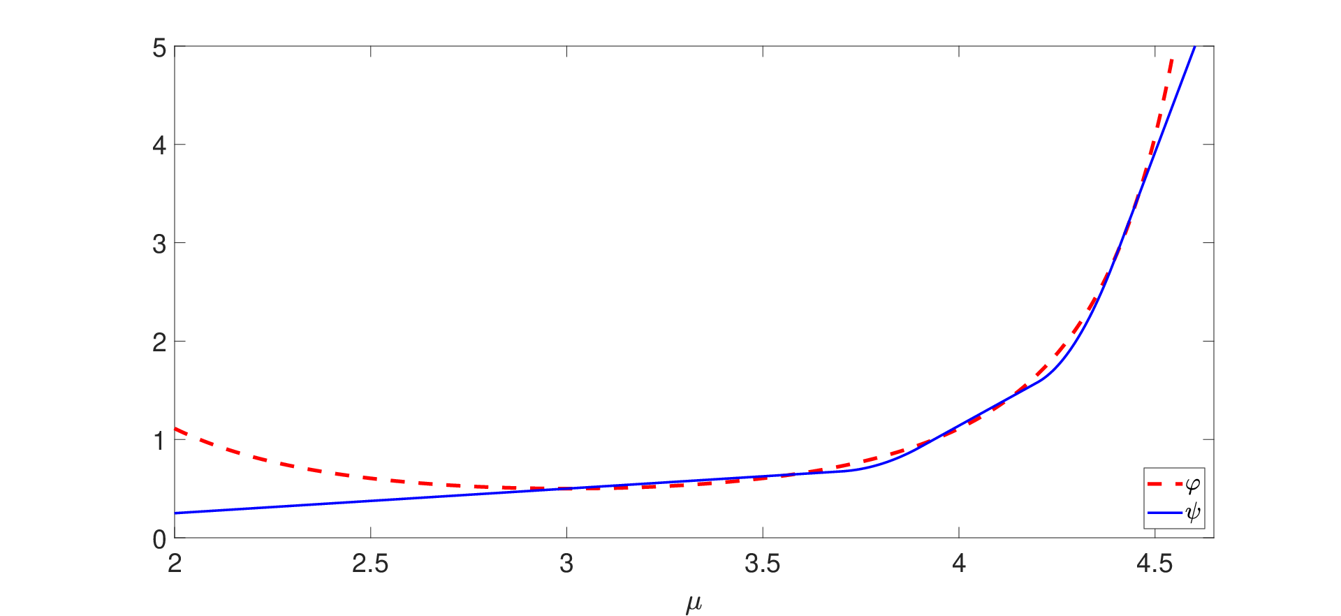
Refer to caption
Figure 2: Variations of φ⁡(μ)\varphi(\mu) and ψ⁡(μ)\psi(\mu) in Example 5.2.

Now, we are interested in when (40) has at most one local non-global minimizer, and whether(40) could have necessary and sufficient optimality condition at local non-global minimizer. The proof is a combination of those of Theorem 3.2 in [13] and Theorem 3.1 in [23].

Theorem 5.3

Suppose f0​(y)f_{0}(y) is thrice continuously differentiable and strongly convex in SS and ψ⁡(μ)\psi(\mu) defined in (42) is log-concave in (max⁡{−λ2,0},−λ1)(\max\{-\lambda_{2},0\},-\lambda_{1}), then

(i) (40) has at most one local non-global minimizer.

(ii) (x∗,y∗)(x_{*},y_{*}) is a local non-global minimizer of (40) if and only if

(H+μ∗​I)​x∗+c=0,f0′​(y∗)−a​μ∗2=0,(H+\mu^{*}I)x_{*}+c=0,~f^{\prime}_{0}(y_{*})-\tfrac{a\mu^{*}}{2}=0, (44)

where μ∗\mu^{*} is a root of the scalar function ϕ⁡(μ)\phi(\mu) defined in (39) in (max⁡{−λ2,0},−λ1)(\max\{-\lambda_{2},0\},-\lambda_{1}) such that ϕ′​(μ∗)>0\phi^{\prime}(\mu^{*})>0.

Proof. (i) We first observe that the scalar function ϕ⁡(μ)\phi(\mu) in (39) has the same roots as

p⁡(μ)=ln⁡φ⁡(μ)−ln⁡ψ⁡(μ),μ∈(max⁡{−λ2,0},−λ1).p(\mu)=\ln\varphi(\mu)-\ln\psi(\mu),~\mu\in(\max\{-\lambda_{2},0\},-\lambda_{1}).

By Theorem 3.4, it is necessary to assume g1≠0g_{1}\neq 0. Using chain rule, (19) gives

p′′​(μ)=[∑i=1n6​gi2(λi+μ)4]​[∑i=1ngi2(λi+μ)2]−[∑i=1n2​gi2(λi+μ)3]2[φ⁡(μ)]2−(ln⁡ψ⁡(μ))′′.p^{\prime\prime}(\mu)=\frac{\left[\sum_{i=1}^{n}\frac{6g_{i}^{2}}{(\lambda_{i}+\mu)^{4}}\right]\left[\sum_{i=1}^{n}\frac{g_{i}^{2}}{(\lambda_{i}+\mu)^{2}}\right]-{\left[\sum_{i=1}^{n}\frac{2g_{i}^{2}}{{(\lambda_{i}+\mu)}^{3}}\right]}^{2}}{[\varphi(\mu)]^{2}}-{\left(\ln\psi(\mu)\right)}^{\prime\prime}.

Define two vectors in ℝn{\mathbb{R}}^{n}:

s=[6​g1(λ1+μ)2,⋯,6​gn(λn+μ)2]T,t=[g1λ1+μ,⋯,gnλn+μ]Ts=\begin{bmatrix}\frac{\sqrt{6}g_{1}}{{(\lambda_{1}+\mu)}^{2}},\cdots,\frac{\sqrt{6}g_{n}}{{(\lambda_{n}+\mu)}^{2}}\end{bmatrix}^{T},~t=\begin{bmatrix}\frac{g_{1}}{\lambda_{1}+\mu},\cdots,\frac{g_{n}}{\lambda_{n}+\mu}\end{bmatrix}^{T}

It follows from Cauchy-Schwartz inequality that

[∑i=1n2​gi2(λi+μ)3]2<(sT​t)2≤(sT​s)​(tT​t)=[∑i=1n6​gi2(λi+μ)4]​[∑i=1ngi2(λi+μ)2].{\left[\sum_{i=1}^{n}\frac{2g_{i}^{2}}{{(\lambda_{i}+\mu)}^{3}}\right]}^{2}<{(s^{T}t)}^{2}\leq(s^{T}s)(t^{T}t)=\left[\sum_{i=1}^{n}\frac{6g_{i}^{2}}{{(\lambda_{i}+\mu)}^{4}}\right]\left[\sum_{i=1}^{n}\frac{g_{i}^{2}}{{(\lambda_{i}+\mu)}^{2}}\right].

The assumption that ψ⁡(μ)\psi(\mu) is log-concave implies that (ln⁡ψ⁡(μ))′′≤0{\left(\ln\psi(\mu)\right)}^{\prime\prime}\leq 0. Therefore, we have p′′​(μ)>0p^{\prime\prime}(\mu)>0 and hence p⁡(μ)p(\mu) is strictly convex for all μ∈(max⁡{−λ2,0},−λ1)\mu\in(\max\{-\lambda_{2},0\},-\lambda_{1}). Thus the equation p⁡(μ)=0p(\mu)=0, as well as ϕ⁡(μ)=0\phi(\mu)=0, has at most two real roots in the above interval, denoted by μ1<μ2\mu_{1}<\mu_{2}. Suppose ϕ′​(μ1)≥0\phi^{\prime}(\mu_{1})\geq 0 and ϕ′​(μ2)≥0\phi^{\prime}(\mu_{2})\geq 0. Then, for any sufficiently small ϵ∈(0,(μ2−μ1)/2)\epsilon\in(0,(\mu_{2}-\mu_{1})/2), we have

ϕ⁡(μ1+ϵ)≥ϕ⁡(μ1)=0,ϕ⁡(μ2−ϵ)≤ϕ⁡(μ2)=0.\phi(\mu_{1}+\epsilon)\geq\phi(\mu_{1})=0,~\phi(\mu_{2}-\epsilon)\leq\phi(\mu_{2})=0.

Therefore, there is a μ~∈[μ1+ϵ,μ2−ϵ]\tilde{\mu}\in[\mu_{1}+\epsilon,\mu_{2}-\epsilon] such that ϕ⁡(μ~)=0\phi(\tilde{\mu})=0, which is a contradiction. Consequently, the scalar function ϕ⁡(μ)\phi(\mu) has at most one real root satisfying ϕ′​(μ)≥0\phi^{\prime}(\mu)\geq 0. Following Theorem 4.4, the proof is complete.

(ii) Firstly, we prove that the assumption that ψ⁡(μ)\psi(\mu) is log-concave in (max⁡{−λ2,0},−λ1)(\max\{-\lambda_{2},0\},-\lambda_{1}) is equivalent to

f0′′′​(y⁡(μ))+aa​y​(μ)+b​f0′′​(y⁡(μ))≥0,μ∈(max⁡{−λ2,0},−λ1).\displaystyle f_{0}^{\prime\prime\prime}(y(\mu))+\frac{a}{ay(\mu)+b}f_{0}^{\prime\prime}(y(\mu))\geq 0,\mu\in(\max\{-\lambda_{2},0\},-\lambda_{1}). (45)

Applying the inverse function theorem to (41), one can verify that

y′(μ)=a2​f0′′​(y⁡(μ)),y′′(μ)=−a​f0′′′​(y⁡(μ))​y′​(μ)2​(f0′′​(y⁡(μ)))2.\begin{array}[]{ll}y^{\prime}(\mu)=\frac{a}{2f^{\prime\prime}_{0}(y(\mu))},~y^{\prime\prime}(\mu)=-\frac{af^{\prime\prime\prime}_{0}(y(\mu))y^{\prime}(\mu)}{2(f^{\prime\prime}_{0}(y(\mu)))^{2}}.\end{array}

Combining with (42),

(ln⁡(ψ⁡(μ)))′′=ψ′′​(μ)​ψ​(μ)−(ψ′​(μ))2(ψ⁡(μ))2=−a34​(a​y​(μ)+b)​[f0′′​(y⁡(μ))]3​[f0′′′​(y⁡(μ))+aa​y​(μ)+b​f0′′​(y⁡(μ))].\begin{array}[]{ll}(\ln(\psi(\mu)))^{\prime\prime}&=\frac{\psi^{\prime\prime}(\mu)\psi(\mu)-{(\psi^{\prime}(\mu))}^{2}}{{(\psi(\mu))}^{2}}\\ &=-\frac{a^{3}}{4(ay(\mu)+b){[f_{0}^{\prime\prime}(y(\mu))]}^{3}}[f_{0}^{\prime\prime\prime}(y(\mu))+\frac{a}{ay(\mu)+b}f_{0}^{\prime\prime}(y(\mu))].\end{array}

which implies (45).

It is sufficient to prove that the optimality condition in Theorem 4.5 is necessary, if (45) hold. Let (x∗,y∗)(x_{*},y_{*}) be a local non-global minimizer of (40). It follows from Theorem 4.4 and the discussion after Theorem 4.5 that (44) holds and μ∗\mu^{*} is a root of the scalar function ϕ\phi in (max⁡{−λ2,0},−λ1)(\max\{-\lambda_{2},0\},-\lambda_{1}) such that ϕ′​(μ∗)≥0\phi^{\prime}(\mu^{*})\geq 0. The remaining part is to show ϕ′​(μ∗)>0\phi^{\prime}(\mu^{*})>0. Suppose this is not true, that is, we assume ϕ′​(μ∗)=0\phi^{\prime}(\mu^{*})=0. According to (32), the reduced Hessian

B:=WT​G​WB:=W^{T}GW

has a zero eigenvalue, where

G=[H+μ∗​I00f0′′​(y∗)],W=[V001]​[g2λ2+μ∗g3λ3+μ∗⋯gnλn+μ∗a2−g1λ1+μ∗0⋯000−g1λ1+μ∗⋯0000⋯−g1λ1+μ∗000⋯0−g1λ1+μ∗].G=\begin{bmatrix}H+\mu^{*}I&0\\ 0&f_{0}^{\prime\prime}(y_{*})\end{bmatrix},~W=\begin{bmatrix}V&0\\ 0&1\end{bmatrix}\begin{bmatrix}\frac{g_{2}}{\lambda_{2}+\mu^{*}}&\frac{g_{3}}{\lambda_{3}+\mu^{*}}&\cdots&\frac{g_{n}}{\lambda_{n}+\mu^{*}}&\frac{a}{2}\\ -\frac{g_{1}}{\lambda_{1}+\mu^{*}}&0&\cdots&0&0\\ 0&-\frac{g_{1}}{\lambda_{1}+\mu^{*}}&\cdots&0&0\\ \vdots&\vdots&&\vdots&\vdots\\ 0&0&\cdots&-\frac{g_{1}}{\lambda_{1}+\mu^{*}}&0\\ 0&0&\cdots&0&-\frac{g_{1}}{\lambda_{1}+\mu^{*}}\end{bmatrix}. (46)

Let q≠0q\neq 0 be an eigenvector of BB corresponding to the zero eigenvalue. That is,

WT​G​W​q=0.W^{T}GWq=0. (47)

Since columns of WW form a basis of the hyperplane x∗T​s−a2​t=0x_{*}^{T}s-\tfrac{a}{2}t=0, i.e.,

WT​[x∗T−a2]T=0,W^{T}\begin{bmatrix}x_{*}^{T}&-\tfrac{a}{2}\end{bmatrix}^{T}=0,

and WW is of full column rank. It follows from (47) that

G​W​q=γ​[x∗−a2]GWq=\gamma\begin{bmatrix}x_{*}\\ -\tfrac{a}{2}\end{bmatrix} (48)

for some γ∈ℝ\gamma\in{\mathbb{R}}. It follows from the linearly independence of columns of WW and q≠0q\neq 0 that

W​q≠0.Wq\neq 0. (49)

Notice that the matrix GG in (46) is nonsingular. By combining (48) and (49), we have

W​q=γ​G−1​[x∗−a2]=:[s∗t∗],Wq=\gamma G^{-1}\begin{bmatrix}x_{*}\\ -\tfrac{a}{2}\end{bmatrix}=:\begin{bmatrix}s_{*}\\ t_{*}\end{bmatrix}, (50)

where s∗∈ℝn,t∗∈ℝs_{*}\in{\mathbb{R}}^{n},t_{*}\in{\mathbb{R}}. Thus γ≠0\gamma\neq 0. Furthermore, we claim that s∗≠0,t∗≠0s_{*}\neq 0,t_{*}\neq 0 and

t∗=2a​x∗T​s∗.t_{*}=\frac{2}{a}x_{*}^{T}s_{*}. (51)

Actually, substituting the matrix GG defined in (46) into the second equality of (50) yields t∗=−γ​a2​f0′′​(y)≠0t_{*}=-\tfrac{\gamma a}{2f^{\prime\prime}_{0}(y)}\neq 0. Multiplying qT​WTq^{T}W^{T} from left to both sides of (48) gives

0=qT​WT​G​W​q=γ⁡(s∗T​x∗−a​t∗2),0=q^{T}W^{T}GWq=\gamma(s_{*}^{T}x_{*}-\tfrac{at_{*}}{2}),

where the first equality holds from (47). Now we obtain (51). Since t∗≠0t_{*}\neq 0, it follows from (51) that s∗≠0s_{*}\neq 0. Define

y⁡(β):=‖x∗+β​s∗‖2−ba,h⁡(β):=q⁡(x∗+β​s∗)+f0​(y⁡(β)).y(\beta):=\tfrac{\|x_{*}+\beta s_{*}\|^{2}-b}{a},~h(\beta):=q(x_{*}+\beta s_{*})+f_{0}(y(\beta)).

One can verify that

h′​(β)=s∗T∇q(x∗+βs∗)+f′0(y(β))y′(β),h′′​(β)=s∗T​∇2q​(x∗+β​s∗)​s∗+f0′′​(y⁡(β))​[y′​(β)]2+f0′​(y⁡(β))​y′′​(β),h′′′​(β)=f0′′′​(y⁡(β))​[y′​(β)]3+3​f0′′​(y⁡(β))​y′​(β)​y′′​(β)+f0′​(y⁡(β))​y′′′​(β),\begin{array}[]{ll}h^{\prime}(\beta)&=s_{*}^{T}\nabla q(x_{*}+\beta s_{*})+f^{\prime}_{0}(y(\beta))y^{\prime}(\beta),\\ h^{\prime\prime}(\beta)&=s_{*}^{T}\nabla^{2}q(x_{*}+\beta s_{*})s_{*}+f^{\prime\prime}_{0}(y(\beta))[y^{\prime}(\beta)]^{2}+f^{\prime}_{0}(y(\beta))y^{\prime\prime}(\beta),\\ h^{\prime\prime\prime}(\beta)&=f^{\prime\prime\prime}_{0}(y(\beta))[y^{\prime}(\beta)]^{3}+3f^{\prime\prime}_{0}(y(\beta))y^{\prime}(\beta)y^{\prime\prime}(\beta)+f^{\prime}_{0}(y(\beta))y^{\prime\prime\prime}(\beta),\end{array}

and y⁡(0)=y∗,y′​(0)=t∗,y′′​(0)=2​s∗T​s∗a,y′′′​(0)=0y(0)=y_{*},y^{\prime}(0)=t_{*},y^{\prime\prime}(0)=\tfrac{2s_{*}^{T}s_{*}}{a},y^{\prime\prime\prime}(0)=0. Let β=0\beta=0,

h′​(0)=s∗T​(H​x∗+c)+f0′​(y∗)​t∗,h′′​(0)=s∗T​H​s∗+f0′′​(y∗)​t∗2+f0′​(y∗)​2​s∗T​s∗a=qT​WT​G​W​q,h′′′​(0)=f0′′′​(y∗)​t∗3+3​f0′′​(y∗)​t∗​2​s∗T​s∗a,\begin{array}[]{ll}h^{\prime}(0)&=s_{*}^{T}(Hx_{*}+c)+f^{\prime}_{0}(y_{*})t_{*},\\ h^{\prime\prime}(0)&=s_{*}^{T}Hs_{*}+f^{\prime\prime}_{0}(y_{*})t_{*}^{2}+f^{\prime}_{0}(y_{*})\tfrac{2s_{*}^{T}s_{*}}{a}=q^{T}W^{T}GWq,\\ h^{\prime\prime\prime}(0)&=f^{\prime\prime\prime}_{0}(y_{*})t_{*}^{3}+3f^{\prime\prime}_{0}(y_{*})t_{*}\tfrac{2s_{*}^{T}s_{*}}{a},\end{array}

where the second equality on h′′​(0)h^{\prime\prime}(0) follows from (44), (46) and (50). The first-order necessary optimality condition (44) and (51) implies h′​(0)=0h^{\prime}(0)=0. According to the definition of qq in (47), we have h′′​(0)=0h^{\prime\prime}(0)=0. Notice that t∗≠0t_{*}\neq 0. Substituting (51) and x∗T​x∗=a​y∗+bx_{*}^{T}x_{*}=ay_{*}+b into h′′′​(0)h^{\prime\prime\prime}(0) yields that

h′′′​(0)t∗3=f0′′′​(y∗)+6​f0′′​(y∗)​s∗T​s∗a​t∗2=f0′′′​(y∗)+3​a​f0′′​(y∗)2​(a​y∗+b)​s∗T​s∗​x∗T​x∗(x∗T​s∗)2≥f0′′′​(y∗)+3​a​f0′′​(y∗)2​(a​y∗+b)>0,\frac{h^{\prime\prime\prime}(0)}{t_{*}^{3}}=f^{\prime\prime\prime}_{0}(y_{*})+6f^{\prime\prime}_{0}(y_{*})\frac{s_{*}^{T}s_{*}}{at_{*}^{2}}=f^{\prime\prime\prime}_{0}(y_{*})+\frac{3af^{\prime\prime}_{0}(y_{*})}{2(ay_{*}+b)}\frac{s_{*}^{T}s_{*}x_{*}^{T}x_{*}}{(x_{*}^{T}s_{*})^{2}}\geq f^{\prime\prime\prime}_{0}(y_{*})+\frac{3af^{\prime\prime}_{0}(y_{*})}{2(ay_{*}+b)}>0,

where the last two inequalities follow from Cauchy-Schwartz inequality, (45) and aa​y​(μ)+b​f0′′​(y⁡(μ))>0\tfrac{a}{ay(\mu)+b}f^{\prime\prime}_{0}(y(\mu))>0. Note that the first inequality also needs the fact a>0a>0. We obtain h′′′​(0)≠0h^{\prime\prime\prime}(0)\neq 0, which contradicts the facts that (x∗+β​s∗,y⁡(β))(x_{*}+\beta s_{*},y(\beta)) is feasible for (40) for all β∈ℝ\beta\in{\mathbb{R}}, and (x∗,y∗)(x_{*},y_{*}) is a local minimizer of (40). Therefore, ϕ′​(μ∗)>0\phi^{\prime}(\mu^{*})>0, the proof of the necessary part is complete.   

Figures (3a) and (3b) illustrate the functions ln⁡ψ⁡(μ)\ln\psi(\mu) and ln⁡φ⁡(μ)\ln\varphi(\mu) for Examples 5.1 and 5.2, respectively. One can observe that in both cases ln⁡ψ⁡(μ)\ln\psi(\mu) is not concave, which implies the necessity of the log-concavity assumption in Theorem 5.3.

Refer to caption
(a) Example 5.1
Refer to caption
(b) Example 5.2
Figure 3: Variants of ln⁡φ⁡(μ)\ln\varphi(\mu) and ln⁡ψ⁡(μ)\ln\psi(\mu) in Examples 5.1 and 5.2.

Finally, we present some examples of f0​(y)f_{0}(y) satisfying the assumptions in Theorem 5.3.

Corollary 5.4

Problem (40) has at most one local non-global minimizer with necessary and sufficient optimality condition for the local non-global minimizer, if one of following conditions holds:

  1. (i)

    f0​(y)=α​yd,α>0,d>1,a=1,b=0f_{0}(y)=\alpha y^{d},~\alpha>0,~d>1,~a=1,~b=0, (which includes Problem (1) as a special case).

  2. (ii)

    f0​(y)f_{0}(y) is a strongly convex quadratic function, a>0,b≥0a>0,~b\geq 0.

  3. (iii)

    f0​(y)f_{0}(y) is a strongly convex cubic polynomial function in (0,+∞)(0,+\infty), a=1,b=0a=1,~b=0.

Proof. According to Theorem 5.3, we only need to verify that (45) holds for each case.

(i) f0​(y)=α​yd,f0′​(y)=α​d​yd−1,f0′′​(y)=α​d​(d−1)​yd−2,f0′′′​(y)=α​d​(d−1)​(d−2)​yd−3.f_{0}(y)=\alpha y^{d},\ f^{\prime}_{0}(y)=\alpha dy^{d-1},\ f^{\prime\prime}_{0}(y)=\alpha d(d-1)y^{d-2},\ f^{\prime\prime\prime}_{0}(y)=\alpha d(d-1)(d-2)y^{d-3}.

f0′′′​(y)+1y​f0′′​(y)=α​d​(d−1)2​yd−3>0,∀y∈(0,+∞),f^{\prime\prime\prime}_{0}(y)+\frac{1}{y}f^{\prime\prime}_{0}(y)=\alpha d{(d-1)}^{2}y^{d-3}>0,\ \forall y\in(0,+\infty),

which implies that the assumption of Theorem 5.3 holds.

(ii) Without loss of generality, we assume f0​(y)=α​y2+β​y,α>0f_{0}(y)=\alpha y^{2}+\beta y,~\alpha>0. Then f0′​(y)=2​α​y+β,f0′′​(y)=2​α,f0′′′​(y)=0f^{\prime}_{0}(y)=2\alpha y+\beta,f^{\prime\prime}_{0}(y)=2\alpha,f^{\prime\prime\prime}_{0}(y)=0.

f0′′′​(y)+aa​y+b​f0′′​(y)=2​a​αa​y+b>0,∀y∈(−ba,+∞).f^{\prime\prime\prime}_{0}(y)+\frac{a}{ay+b}f^{\prime\prime}_{0}(y)=\frac{2a\alpha}{ay+b}>0,~\forall y\in(-\tfrac{b}{a},+\infty).

(iii) Assume that f0​(y)=α​y3+β​y2+γ​yf_{0}(y)=\alpha y^{3}+\beta y^{2}+\gamma y is strongly convex on (0,+∞)(0,+\infty). Notice that

f0′​(y)=3​α​y2+2​β​y+γ,f0′′​(y)=6​α​y+2​β,f0′′′​(y)=6​α.f^{\prime}_{0}(y)=3\alpha y^{2}+2\beta y+\gamma,\ f^{\prime\prime}_{0}(y)=6\alpha y+2\beta,\ f^{\prime\prime\prime}_{0}(y)=6\alpha.

Since f0′′​(y)=6​α​(y+β3​α)>0,∀y∈(0,+∞)f^{\prime\prime}_{0}(y)=6\alpha\left(y+\frac{\beta}{3\alpha}\right)>0,~\forall y\in(0,+\infty). It turns out that α>0\alpha>0 and β>0\beta>0.

f0′′′​(y)+1y​f0′′​(y)>0+0=0,∀y∈(0,+∞).f^{\prime\prime\prime}_{0}(y)+\frac{1}{y}f^{\prime\prime}_{0}(y)>0+0=0,~\forall y\in(0,+\infty).


Note that we cannot extend the above cases presented in Corollary 5.4 to the general quartic polynomial case, see Example 5.1 for a counterexample.

6 Conclusion

We raise a fundamental question (Question 1.1) whether local optimality can be checked in polynomial time for hidden convex optimization. Then we focus on the newly proposed optimization problem by jointing nonconvex trust-region subproblem with convex optimization (TRS-C). We present a necessary and sufficient optimality condition for global minimizer of (TRS-C), which reveals its hidden convexity. However, it is difficult to establish a necessary and sufficient optimality condition for local non-global minimizer, except for some quadratic single-constraint cases. Moreover, different from trust region subproblem (which has at most one local non-global minimizer) and convex optimization (without local non-global minimizer), their joint problem could have more than one local non-global minimizer. There is a quartic polynomial case of (TRS-C) with two local non-global minimizers. We then present a general approach to generate the instances with arbitrary number of local non-global minimizers. Consequently, we conclude that the existence of many local minimizers is NOT a (or at least not a unique) reason making global optimization difficult.

While we have present some negative evidences, Question 1.1 remains open, even on the joint problem problem (TRS-C).

Acknowledgments.

This research was supported by the National Natural Science Foundation of China under grants 11822103, 11571029, and 11771056, and by the Beijing Natural Science Foundation, grant Z180005.

References

  • Beck and Pan [2017] Beck A, Pan D (2017) A branch and bound algorithm for nonconvex quadratic optimization with ball and linear constraints. J. Glob. Optim. 69(2):309–342.
  • Boyd and Vandenberghe [2004] Boyd S, Vandenberghe L (2004) Convex Optimization (Cambridge University Press).
  • Bubeck [2015] Bubeck S (2015) Convex optimization: Algorithms and complexity. Foundations and Trends in Machine Learning 8(3-4):231–357, ISSN 1935-8237, URL http://dx.doi.org/10.1561/2200000050.
  • Cartis et al. [2011] Cartis C, Gould NIM, Toint PL (2011) Adaptive cubic regularisation methods for unconstrained optimization. part i: motivation, convergence and numerical results. Mathematical Programming 127(2):245–295.
  • Conn et al. [2000] Conn AR, Gould NIM, Toint PL (2000) Trust Region Methods (Society for Industrial and Applied Mathematics), URL http://dx.doi.org/10.1137/1.9780898719857.
  • Fang et al. [2017] Fang SC, Gao DY, Lin GX, Sheu RL, Xing WX (2017) Double well potential function and its optimization in the nn-dimensional real space - part i. Journal of Industrial and Management Optimization 13(3):1291–1305.
  • Fletcher [1984] Fletcher R (1984) Linear and Nonlinear Programming, 2nd ed. (Reading, MA: Addison-Wesley).
  • Fletcher [1987] Fletcher R (1987) Practical Methods of Optimization, 2nd ed. (New York: John Wiley).
  • Gay [1981] Gay DM (1981) Computing optimal locally constrained steps. SIAM Journal on Scientific and Statistical Computing 2(2):186–197, URL http://dx.doi.org/10.1137/0902016.
  • Golub and Loan [1989] Golub GH, Loan CFV (1989) Matrix Computations, 2nd ed. (Baltimore: The Johns Hopkins University Press).
  • Gould et al. [2010] Gould NIM, Robinson DP, Thorne HS (2010) On solving trust-region and other regularised subproblems in optimization. Mathematical Programming Computation 2(1):21–57.
  • Griewank [1981] Griewank A (1981) The modification of newton’s method for unconstrained optimization by bounding cubic terms. Technical Report DAMTP/NA12 .
  • Hsia et al. [2017] Hsia Y, Sheu RL, Yuan YX (2017) Theory and application of p-regularized subproblems for p>2p>2. Optimization Methods and Software 32(5):1059–1077, ISSN 1055-6788, URL http://dx.doi.org/10.1080/10556788.2016.1238917.
  • Lucidi et al. [1998] Lucidi S, Palagi L, Roma M (1998) On some properties of quadratic programs with a convex quadratic constraint. SIAM Journal on Optimization 8(1):105–122, URL http://dx.doi.org/10.1137/S1052623494278049.
  • Martínez [1994] Martínez JM (1994) Local minimizers of quadratic functions on euclidean balls and spheres. SIAM Journal on Optimization 4(1):159–176, URL http://dx.doi.org/10.1137/0804009.
  • Moré and Sorensen [1983] Moré JJ, Sorensen DC (1983) Computing a trust region step. Siam Journal on Scientific and Statistical Computing 4(3):553–572.
  • Murty and Kabadi [1987] Murty KG, Kabadi SN (1987) Some np-complete problems in quadratic and nonlinear programming. Math. Program. 39(2):117–129.
  • Nesterov [2018] Nesterov Y (2018) Lectures on Convex Optimization (Cham: Springer International Publishing), ISBN 1931-6836, URL http://dx.doi.org/https://doi.org/10.1007/978-3-319-91578-4.
  • Nesterov and Polyak [2006] Nesterov Y, Polyak BT (2006) Cubic regularization of newton method and its global performance. Mathematical Programming 108(1):177–205.
  • Pardalos and Schnitger [1988] Pardalos PM, Schnitger G (1988) Checking local optimality in constrained quadratic programming is np-hard. Oper. Res. Lett. 7(2):33–45.
  • Sorensen [1982] Sorensen DC (1982) Newton’s method with a model trust region modification. SIAM Journal on Numerical Analysis 19(2):409–426.
  • Tao and An [1998] Tao PD, An LTH (1998) A d.c. optimization algorithm for solving the trust-region subproblem. SIAM Journal on Optimization 8(2):476–505, URL http://dx.doi.org/10.1137/S1052623494274313.
  • Wang and Xia [2020] Wang J, Xia Y (2020) Closing the gap between necessary and sufficient conditions for local nonglobal minimizer of trust region subproblem. SIAM Journal on Optimization 30(3):1980–1995, URL http://dx.doi.org/10.1137/19M1294459.
  • Weiser et al. [2007] Weiser M, Deuflhard P, Erdmann B (2007) Affine conjugate adaptive newton methods for nonlinear elastomechanics. Optimization Methods And Software 22(3):413–431.
  • Xia [2020] Xia Y (2020) A survey of hidden convex optimization. J. Oper. Res. Soc. China. 8(2):1–28.
  • Xia et al. [2017] Xia Y, Sheu RL, Fang SC, Xing W (2017) Double well potential function and its optimization in the nn-dimensional real space - part ii. Journal of Industrial and Management Optimization 13(3):1307–1328.
  • Ye [1992] Ye Y (1992) A new complexity result on minimization of a quadratic function with a sphere constraint (Princeton University Press).
  • Yuan [2015] Yuan YX (2015) Recent advances in trust region algorithms. Mathematical Programming 151(1):249–281.