跳到论文正文
W Papers独立论文阅读器 arXiv:2109.03017 论文正文 计算阅读时间 · 0%
引用这篇论文根据当前论文元数据生成,正式投稿前建议核对。


License: arXiv.org perpetual non-exclusive license
arXiv:2109.03017v1 [math.ST] 07 Sep 2021

Estimation of the covariate conditional tail expectation : a depth-based level set approach

Elisabeth Armaut   Roland Diel   Thomas Laloë Thanks: armaut@unice.fr Note: diel@unice.fr Note: laloe@unice.fr Affiliation: Université de Nice Sophia-Antipolis, Laboratoire J-A Affiliation: Dieudonné, Parc Valrose, 06108 Nice Cedex 02, France

Abstract. The aim of this paper is to study the asymptotic behavior of a particular multivariate risk measure, the Covariate-Conditional-Tail-Expectation (CCTE\CCTE), based on a multivariate statistical depth function. Depth functions have become increasingly powerful tools in nonparametric inference for multivariate data, as they measure a degree of centrality of a point with respect to a distribution. A multivariate risks scenario is then represented by a depth-based lower level set of the risk factors, meaning that we consider a non-compact setting. More precisely, given a probability measure PP on ℝd\mathbb{R}^{d} and a depth function D⁡(⋅,P)D(\cdot,P), we are interested in the α\alpha-lower level set ℒD​(α):={z∈ℝd:D⁡(z,P)≤α}\mathcal{L}_{D}(\alpha):=\left\{z\in\mathbb{R}^{d}:D(z,P)\leq\alpha\right\}. First, we present a plug-in approach in order to estimate ℒD​(α).\mathcal{L}_{D}(\alpha). In a second part, we provide a consistent estimator of our CCTE\CCTE for a general depth function with a rate of convergence, and we consider the particular case of the Mahalanobis depth. A simulation study complements the performances of our estimator.

Key-Words. Plug-in estimation, multivariate depth function, Mahalanobis depth, risk theory.

1 Introduction

Risk theory is a branch of statistics which mainly focuses on unlikely events in the aim of managing the degree of uncertainty of such events and/or the associated costs. For instance, in the context of risk management in financial institutions such as banks or insurance companies, adverse consequences may occur and usually mean potential large losses on a portfolio of assets (Eberlein et al., 2007). In hydrology, risk could represent dam floods (and/or failures) and the associated risk factors could be the amount of rainfall, water flow… Broadly speaking, a risk measure can be viewed as a mapping from a set of real-valued random variables to ℝd\mathbb{R}^{d}, d≥1d\geq 1, and is used to determine the amount of an asset (or assets/goods) to be kept in reserve in order to cover for unexpected losses. One of the most studied risk measure in the univariate risk theory is the Conditional-Tail-Expectation (CTE\CTE) (Denuit et al., 2006). It characterizes the conditional expected loss given that the loss exceeds a critical loss threshold. Formally, given a real random variable XX with distribution function FXF_{X}, the CTE\CTE at level α∈(0,1)\alpha\in(0,1) is defined as :

CTEα(X):=𝔼⁡[X|X>VaR(α)],{\CTE}_{\alpha}(X):=\mathbb{E}[X|X>\VaR(\alpha)], (1.1)

where

VaR(α):=inf{t∈ℝ:FX​(t)≥α}\VaR(\alpha):=\inf\left\{t\in\mathbb{R}:F_{X}(t)\geq\alpha\right\}

is the well-known Value at Risk which corresponds to the univariate quantile of order α\alpha of XX. Thus, the CTE\CTE is nothing but the mathematical description of an average loss in the worst 100​(1−α)%100(1-\alpha)\% risk scenario.

However, considering a single risk factor is restrictive, as we can easily imagine correlated risk factors that could be studied together. One possibility is to consider quantile regions of the risk factors distribution. In the univariate case, a wide panel of univariate quantiles has been reviewed in the literature. When it comes to multivariate risks, the study of multivariate quantile regions has increasingly been pursued in the last decades as a tool to model multivariate risk regions, especially those based on a multivariate distribution function (Belzunce et al., 2007, Dehaan and Huang, 1995, Cousin and Di Bernardino, 2013), or on a depth function (Zuo and Serfling, 2000). In this way, several generalizations in higher dimension of the CTE\CTE emerged in the literature. In particular, one can mention the one proposed by Di Bernardino et al., 2013 : given a random vector 𝑿∈ℝd\bm{X}\in\mathbb{R}^{d}, 𝑿=(X1,⋯,Xd)∈ℝd\bm{X}=(X_{1},\cdots,X_{d})\in\mathbb{R}^{d}, d≥1d\geq 1, with mutivariate distribution function F𝑿:ℝd→[0,1]F_{\bm{X}}:\mathbb{R}^{d}\to[0,1], a generalization of the CTE\CTE in higher dimension is defined by

CTEα(𝑿)\displaystyle{\CTE}_{\alpha}(\bm{X}) =𝔼⁡[𝑿|𝑿∈ℒF𝑿​(α)]∈ℝd,\displaystyle=\mathbb{E}[\bm{X}|\bm{X}\in\mathcal{L}_{F_{\bm{X}}}(\alpha)]\in\mathbb{R}^{d}, (1.2)

where

ℒF𝑿​(α):={x∈ℝd:F𝑿​(x)≥α},α∈(0,1),\mathcal{L}_{F_{\bm{X}}}(\alpha):=\left\{x\in\mathbb{R}^{d}:F_{\bm{X}}(x)\geq\alpha\right\},\penalty\ \alpha\in(0,1),

is the α\alpha-upper level set of F𝑿F_{\bm{X}}, which is one generalization of the univariate quantile region [VaRα(X),+∞)[\VaR_{\alpha}(X),+\infty) in dimension d≥1d\geq 1.

Another interesting problem is to study the behavior of an expected cost Y∈ℝY\in\mathbb{R} associated to d≥1d\geq 1 risk factors which are heterogeneous in nature. In econometrics, for instance, one can be interested in an average return (which measures the performance of a portfolio for a certain period of time) with respect to d≥1d\geq 1 risk factors 𝑿∈ℝd\bm{X}\in\mathbb{R}^{d}. On another note, one can also be interested in the impact of climate change (via dd risk factors) on high temperatures. To address this, Di Bernardino et al., 2015 proposed studying the behavior of a covariate variable YY on the level sets of the distribution of a dd-dimensional vector of risk factors 𝑿\bm{X}. More precisely, they define and estimate the multivariate Covariate-conditional-Tail-Expectation (CCTE\CCTE) defined by

CCTEα(Y,𝑿):=𝔼⁡[Y|𝑿∈ℒF𝑿​(α)],α∈(0,1).{\CCTE}_{\alpha}(Y,\bm{X}):=\mathbb{E}[Y|\bm{X}\in\mathcal{L}_{F_{\bm{X}}}(\alpha)],\penalty\ \alpha\in(0,1). (1.3)

However, this CCTE\CCTE based on the distribution function only considers canonical directions. For instance, it could consider an average cost associated to high or low temperatures, but not to high and low temperatures at the same time. Therefore, instead of studying the level sets ℒF𝑿​(α)\mathcal{L}_{F_{\bm{X}}}(\alpha), Torres et al., 2020 studied the level sets ℒFR​𝑿​(α)\mathcal{L}_{F_{R\bm{X}}}(\alpha) of a rotation RR of the distribution. In other words, oriented orthant are considered in order to investigate other risk regions. We propose here a more general approach, consisting in replacing the distribution function by a depth function (see Zuo and Serfling, 2000).

Roughly speaking, a depth function is a mapping

D:ℝd×𝒫⁡(ℝd)→ℝ+D:\mathbb{R}^{d}\times\mathscr{P}(\mathbb{R}^{d})\to\mathbb{R}_{+}

which provides a P𝑿P_{\bm{X}}-based center-outward ordering of points in ℝd,\mathbb{R}^{d}, where 𝒫⁡(ℝd)\mathscr{P}(\mathbb{R}^{d}) denotes the set of all probability measures on ℝd.\mathbb{R}^{d}. Thus, in order to deal with risk regions, we will consider the l​o​w​e​rlower-level sets of a depth function and propose a depth-based CCTE\CCTE defined by :

CCTED,α(Y,𝑿):=𝔼⁡[Y|𝑿∈ℒD​(α)],α>0,\displaystyle{\CCTE}_{D,\alpha}(Y,\bm{X}):=\mathbb{E}[Y|\bm{X}\in\mathcal{L}_{D}(\alpha)],\penalty\ \alpha>0, (1.4)

where ℒD​(α)={x∈ℝd:D⁡(x,P𝑿)≤α}\mathcal{L}_{D}(\alpha)=\left\{x\in\mathbb{R}^{d}:D(x,P_{\bm{X}})\leq\alpha\right\} is the α\alpha-depth based lower level set.

The paper is organized as follows. In Section 2, we introduce some notations, and tools and the mathematical definition of a depth function. Section 3 is devoted to our main results : in Section 3.1, a construction and consistency and convergence rates of an estimator of our CCTED\CCTE_{D} are given in a general setting, in Section 3.2 we study the general asymptotic behavior of our estimator of the level set ℒD​(α)\mathcal{L}_{D}(\alpha), and in Section 3.3 we provide consistency results and convergence rates of the CCTED\CCTE_{D} in the particular case of M​a​h​a​l​a​n​o​b​i​sMahalanobis depth. Illustrations and simulations are presented in Section 4. Finally, proofs are postponed to section 5.

2 Notations and definitions

This section is dedicated to introducing some useful notations and tools.

2.1 General Notations

Let ∅\varnothing be the empty set, ℕ∗=ℕ\{0}\mathbb{N}^{*}=\mathbb{N}\backslash\left\{0\right\} be the set of positive integers, and 𝒫:=𝒫⁡(ℝd)\mathscr{P}:=\mathscr{P}(\mathbb{R}^{d}) be the set of all probability measures on ℝd,\mathbb{R}^{d}, d≥1.d\geq 1. When dealing with random variables, we assume that they are defined on a common underlying probability space (Ω,𝒜,ℙ).(\Omega,\mathscr{A},\mathbb{P}).Given a r.v 𝑿\bm{X} with distribution P𝑿:=P∈𝒫P_{\bm{X}}:=P\in\mathscr{P} and an i.i.d sample Sn:=(𝑿𝒊)1≤i≤nS_{n}:=(\bm{X_{i}})_{1\leq i\leq n} of size n∈ℕ∗n\in\mathbb{N}^{*} with distribution PP and independent of 𝑿\bm{X}, we denote by Pn:=∑i=1nδ𝑿𝒊P_{n}:=\sum_{i=1}^{n}\delta_{\bm{X_{i}}} the empirical measure based on this finite sample. For notational convenience, we denote by 𝔼P\mathbb{E}_{P} the mathematical expectation under PP, and by 𝔼Sn[Z]:=𝔼[Z|𝑿1,⋯,𝑿n]\mathbb{E}_{S_{n}}[Z]:=\mathbb{E}[Z|\bm{X}_{1},\cdots,\bm{X}_{n}] the conditional expectation of ZZ knowing 𝑿1,⋯,𝑿n\bm{X}_{1},\cdots,\bm{X}_{n}. Moreover, denoting Φ⁡(A):=P𝑿​[A]=P⁡[A]\Phi(A):=P_{\bm{X}}[A]=P[A] for any Borel-set A⊂ℝdA\subset\mathbb{R}^{d}, we denote by PSn​[A]:=Φ⁡[A⁡(X1,⋯,Xn)]P_{S_{n}}[A]:=\Phi[A(X_{1},\cdots,X_{n})], where A:=A⁡(X1,⋯,Xn)A:=A(X_{1},\cdots,X_{n}) is a subset of ℝd\mathbb{R}^{d} which depends on the data X1,⋯,XnX_{1},\cdots,X_{n}. Thus, A⁡(X1,⋯,Xn)A(X_{1},\cdots,X_{n}) is a random subset, so that PSn​[A]P_{S_{n}}[A] is a r.v. Furthermore, for any real number q>0q>0, let 𝕃q​(Ω):=𝕃q​(Ω,𝒜,ℙ)\mathbb{L}^{q}(\Omega):=\mathbb{L}^{q}(\Omega,\mathscr{A},\mathbb{P}) denote the vector space of real-valued random variables UU for which 𝔼⁡[|U|q]<+∞\mathbb{E}[|U|^{q}]<+\infty.

Unambiguously, we denote by ∥⋅∥\|\cdot\| the Euclidean norm in ℝd\mathbb{R}^{d} and by |||⋅|||{\left|\kern-1.07639pt\left|\kern-1.07639pt\left|\cdot\right|\kern-1.07639pt\right|\kern-1.07639pt\right|} the matrix norm induced by the Euclidean norm in ℝd,\mathbb{R}^{d}, i.e for any d×dd\times d real matrix MM,

‖|M|‖:=supx≠0‖M​x‖‖x‖=sup‖x‖=1‖M​x‖.{\left|\kern-1.07639pt\left|\kern-1.07639pt\left|M\right|\kern-1.07639pt\right|\kern-1.07639pt\right|}:=\sup_{x\neq 0}\frac{\|Mx\|}{\|x\|}=\sup_{\|x\|=1}\|Mx\|.

For p∈[1,+∞]p\in[1,+\infty], we also denote by

‖f‖p,λ:=(∫ℝd|f⁡(x)|p​𝑑x)1p​ for ​p<+∞, and\displaystyle\|f\|_{p,\lambda}:=\left(\int_{\mathbb{R}^{d}}|f(x)|^{p}dx\right)^{\frac{1}{p}}\text{\penalty\ \penalty\ for\penalty\ }p<+\infty,\text{\penalty\ and}
‖f‖∞,ℝd:=ess supx∈ℝd​|f⁡(x)|​ for ​p=+∞,\displaystyle\|f\|_{\infty,\mathbb{R}^{d}}:=\text{ess sup}_{x\in\mathbb{R}^{d}}|f(x)|\text{\penalty\ \penalty\ for\penalty\ }p=+\infty,

the 𝕃p​(ℝd,λd)\mathbb{L}^{p}(\mathbb{R}^{d},\lambda_{d}) norm of ff w.r.t the Lebesgue measure on ℝd\mathbb{R}^{d}.

We recall that for A and B non-empty compact sets in (ℝd,∥⋅∥)(\mathbb{R}^{d},\|\cdot\|) the Hausdorff distance between A and B is defined by

dH​(A,B)=sup(supa∈Adist(a,B),supb∈Bdist(b,A))d_{H}(A,B)=\displaystyle\sup\left(\sup_{a\in A}\dist(a,B),\sup_{b\in B}\dist(b,A)\right),

where,

dist(x,A):=infa∈A:=∥a−x∥.\dist(x,A):=\displaystyle\inf_{a\in A}:=\|a-x\|.

Now, given two sequences of real numbers (un)n≥1(u_{n})_{n\geq 1} and (vn)n≥1(v_{n})_{n\geq 1}, we recall that un=On​(vn)u_{n}=O_{n}(v_{n}) means that there exist a constant C>0C>0 and N∈ℕ∗N\in\mathbb{N}^{*} s.t. for all n≥N,n\geq N, |un|≤C​|vn||u_{n}|\leq C|v_{n}|.

Finally, let (Xn)n∈(ℕ∗)r(X_{n})_{n\in(\mathbb{N}^{*})^{r}}, r≥1r\geq 1, be a set of random variables and (un)n∈(ℕ∗)r(u_{n})_{n\in(\mathbb{N}^{*})^{r}} be a deterministic set of positive real numbers, we recall the following classical stochastic dominance

𝑿𝒏=𝓞ℙ,𝒏​(𝒖𝒏)⟺def\bm{X_{n}=\mathcal{O}_{\mathbb{P},n}(u_{n})\stackrel{{\scriptstyle\text{def}}}{{\Longleftrightarrow}}}

∀ε>0,\displaystyle\forall\penalty\ \varepsilon>0, ∃Mε>0,∃Nε≥1,∀n:=(n1,⋯,nr)∈(ℕ∗)r,\displaystyle\penalty\ \exists\penalty\ M_{\varepsilon}>0,\penalty\ \exists\penalty\ N_{\varepsilon}\geq 1,\penalty\ \forall\penalty\ n:=(n_{1},\cdots,n_{r})\in(\mathbb{N}^{*})^{r},
min1≤i≤rni≥Nε⇒ℙ[Xn≥Mε⋅un]≤ε.\displaystyle\min_{1\leq i\leq r}n_{i}\geq N_{\varepsilon}\Rightarrow\mathbb{P}[X_{n}\geq M_{\varepsilon}\cdot u_{n}]\leq\varepsilon.

2.2 Depth functions

In this section, we formally introduce the definition of a statistical multivariate depth function as in Zuo and Serfling, 2000 (Definition 2.1 in [16]). Let us begin with some common multivariate symmetry notions which have been widely used in the literature (the interested reader can refer to Zuo and Serfling, 2000, Liu, 1990, and Beran and Millar, 1997). In what follows, we review some standard symmetry notions.

∙\bullet CC-symmetry : a random vector 𝑿∈ℝd\bm{X}\in\mathbb{R}^{d} is centrally-symmetric (or CC-symmetric) about θ∈ℝd\theta\in\mathbb{R}^{d} if 𝑿−θ=dθ−𝑿\bm{X}-\theta\stackrel{{\scriptstyle\rm d}}{{=}}\theta-\bm{X}.

∙\bullet AA-symmetry (Liu, 1990) : 𝑿\bm{X} is said to be angularly-symmetric (or AA-symmetric) about θ\theta, if (𝑿−θ)/‖𝑿−θ‖(\bm{X}-\theta)/\|\bm{X}-\theta\| is centrally symmetric about the origin.

∙\bullet HH-symmetry (Zuo and Serfling, 2000) : 𝑿\bm{X} is said to be halfspace-symmetric (or HH-symmetric) about θ\theta if P𝑿​[H]≥1/2P_{\bm{X}}[H]\geq 1/2 for every closed halfspace HH containing θ\theta.

Note that, it is easily established that CC-symmetry ⇒\Rightarrow AA-symmetry ⇒\Rightarrow HH-symmetry. In a natural terminology, θ\theta is called the center of the distribution P𝑿P_{\bm{X}}.

Definition 2.1 (Zuo and Serfling, 2000).

A statistical depth function is a mapping D:ℝd×𝒫→ℝD:\mathbb{R}^{d}\times\mathscr{P}\to\mathbb{R} which is bounded, non negative, measurable in its first argument and satisfying :
(D1) Affine invariance : for any P𝐗∈𝒫P_{\bm{X}}\in\mathscr{P}, b∈ℝdb\in\mathbb{R}^{d}, and any invertible size dd matrix AA, D⁡(A​x+b,PA​𝐗+b)=D⁡(x,P𝐗)D(Ax+b,P_{A\bm{X}+b})=D(x,P_{\bm{X}})
(D2) Maximality at center : for any P𝐗∈𝒫P_{\bm{X}}\in\mathscr{P} having a unique center θ∈ℝd\theta\in\mathbb{R}^{d} (for one of the symmetry notions previously presented), D⁡(θ,P𝐗)=supx∈ℝdD⁡(x,P𝐗)D(\theta,P_{\bm{X}})=\sup_{x\in\mathbb{R}^{d}}D(x,P_{\bm{X}})
(D3) Monotonicity relative to deepest point : for any P𝐗P_{\bm{X}} having deepest point θ\theta i.e. D⁡(θ,P𝐗)=supx∈ℝdD⁡(x,P𝐗)D(\theta,P_{\bm{X}})=\sup_{x\in\mathbb{R}^{d}}D(x,P_{\bm{X}}), D⁡(x,P𝐗)≤D⁡(α​x+(1−α)​θ,P𝐗)D(x,P_{\bm{X}})\leq D(\alpha x+(1-\alpha)\theta,P_{\bm{X}}) holds for α∈[0,1]\alpha\in[0,1]
(D4) Vanishing at infinity : D⁡(x,P𝐗)→0D(x,P_{\bm{X}})\to 0 as ‖x‖→∞\|x\|\to\infty, for each P𝐗∈𝒫P_{\bm{X}}\in\mathscr{P}.

Informally, the first property of a depth (𝑫​𝟏)\bm{(D1)} suggests that the depth of a point x∈ℝdx\in\mathbb{R}^{d} does not depend on the underlying coordinate system. As far as property (𝑫​𝟐)\bm{(D2)} is concerned, for a distribution having a unique "center" i.e., the point of symmetry with respect to some notion of multivariate symmetry, the depth function should attain its maximum value at this center. Property (𝑫​𝟑)\bm{(D3)} illustrates the fact that as a point x∈ℝdx\in\mathbb{R}^{d} moves away from the point of maximal depth (for instance the "center" of a distribution) along any fixed ray through the center, the depth at xx should decrease monotonically. Last but not least, property (𝑫​𝟒)\bm{(D4)} implies that the depth of a point xx approaches zero as ‖x‖\|x\| approaches infinity. Note that (𝑫​𝟑)\bm{(D3)} and (𝑫​𝟒)\bm{(D4)} mean that the upper level sets

{x∈ℝd:D⁡(x,P𝑿)≥α},α>0,\left\{x\in\mathbb{R}^{d}:D(x,P_{\bm{X}})\geq\alpha\right\},\penalty\ \alpha>0,

are bounded and starshaped about the point of maximum depth.

3 Main results

In this section, we define a risk measure based on a general depth function, the Covariate-Conditional-Tail-Expectation (CCTED\CCTE_{D}) and we propose an estimator of the CCTED\CCTE_{D} using a plug-in estimator of the level set. We study the asymptotic behavior of the CCTED\CCTE_{D} when consistency of the level sets in terms of the probability under P∈𝒫P\in\mathscr{P} of the volume of the symmetric difference is provided.

3.1 General Covariate-Conditional-Tail-Expectation consistency

Fix a depth function D:ℝd×𝒫→ℝD:\mathbb{R}^{d}\times\mathscr{P}\to\mathbb{R} and a distribution P∈𝒫P\in\mathscr{P}. We denote

αmax​(P):=supz∈ℝdD⁡(z,P)=supz∈ℝdD⁡(z).\alpha_{\max}(P):=\sup_{z\in\mathbb{R}^{d}}D(z,P)=\sup_{z\in\mathbb{R}^{d}}D(z).

Consider a couple (Y,𝑿)(Y,\bm{X}) s.t. YY is a real random variable which is dependent on a random vector 𝑿∈ℝd\bm{X}\in\mathbb{R}^{d} with ditribution PP. In Definition 3.1, we formally define our CCTED\CCTE_{D} and propose an estimator of the latter. For n1,n2≥1n_{1},\penalty\ n_{2}\geq 1, let

S~n1:=(𝑿~i)i=1,..,n1​ be an i.i.d ​n1​-sample from ​P, and\displaystyle\tilde{S}_{n_{1}}:=(\tilde{\bm{X}}_{i})_{i=1,..,n_{1}}\text{\penalty\ be an i.i.d\penalty\ }n_{1}\text{-sample from\penalty\ }P,\text{\penalty\ and}
Sn2:=((Yi,𝑿i))i=1,..,n2​ be an i.i.d ​n2​-sample from ​P(Y,𝑿),\displaystyle S_{n_{2}}:=((Y_{i},\bm{X}_{i}))_{i=1,..,n_{2}}\text{\penalty\ be an i.i.d\penalty\ }n_{2}\text{-sample from\penalty\ }P_{(Y,\bm{X})},

s.t. S~n1\tilde{S}_{n_{1}} and Sn2S_{n_{2}} are independent. Now, we define the α\alpha-lower level set of DD and its plug-in estimator based on S~n1\tilde{S}_{n_{1}} by

𝓛𝑫​(𝜶)=𝓛𝑫​(𝜶,𝑷):={𝒙∈ℝ𝒅:𝑫⁡(𝒙,𝑷)≤𝜶},and\displaystyle\bm{\mathcal{L}_{D}(\alpha)}=\bm{\mathcal{L}_{D}(\alpha,P):=\left\{x\in\mathbb{R}^{d}:D(x,P)\leq\alpha\right\},}\text{and}
𝓛𝒏𝟏​(𝜶):=𝓛𝑫​(𝜶,𝑷~𝒏𝟏)={𝒙∈ℝ𝒅:𝑫𝒏𝟏​(𝒙):=𝑫⁡(𝒙,𝑷~𝒏𝟏)≤𝜶},\displaystyle\bm{\mathcal{L}_{n_{1}}(\alpha):=\bm{\mathcal{L}_{D}(\alpha,\tilde{P}_{n_{1}})}=\left\{x\in\mathbb{R}^{d}:D_{n_{1}}(x):=D(x,\tilde{P}_{n_{1}})\leq\alpha\right\}},

where P~n1\tilde{P}_{n_{1}} is the empirical measure based on the sample S~n1:=(𝑿~𝒊)1≤i≤n1\tilde{S}_{n_{1}}:=(\bm{\tilde{X}_{i}})_{1\leq i\leq n_{1}}.
Finally, we provide the definition of our CCTED\CCTE_{D} and its associated estimator.

Definition 3.1 (Depth-based Covariate-Conditional-Tail-Expectation).

Let 𝐗\bm{X} ∈ℝd\in\mathbb{R}^{d} be a random vector with distribution P∈𝒫P\in\mathscr{P} and YY be an integrable real random variable (which is dependent on 𝐗\bm{X}). Let α>0\alpha>0 and assume P​[ℒD​(α)]>0P[\mathcal{L}_{D}(\alpha)]>0.


(i)(i) The depth-based Covariate-Conditionale-Tail-Expectation at level α\alpha is defined by :

CCTED,α(Y,𝑿):=𝔼⁡[Y|𝑿∈ℒD​(α)].{\CCTE}_{D,\alpha}(Y,\bm{X}):=\mathbb{E}[Y|\bm{X}\in\mathcal{L}_{D}(\alpha)].

(i​i)(ii) Its estimator based on the sample Sn2S_{n_{2}} is given by :

CCTE^D,αn1,n2​(Y,𝑿):=∑i=1n2Yi​𝟙𝑿i∈ℒn1​(α)∑i=1n2𝟙𝑿i∈ℒn1​(α),\displaystyle\widehat{\CCTE}_{D,\alpha}^{n_{1},n_{2}}(Y,\bm{X}):=\displaystyle\frac{\displaystyle\sum_{i=1}^{n_{2}}Y_{i}\mathds{1}_{\bm{X}_{i}\in\mathcal{L}_{n_{1}}(\alpha)}}{\displaystyle\sum_{i=1}^{n_{2}}\mathds{1}_{\bm{X}_{i}\in\mathcal{L}_{n_{1}}(\alpha)}}, (3.1)

with the convention 0/0=0.0/0=0.

Our first result, namely Theorem 3.2, links the rate of convergence of the CCTED\CCTE_{D} to the one of the symmetric difference between the true and estimated α\alpha-level set. We first state the following assumption describing a convergence rate for the level sets:


(H0): there exists an increasing sequence of positive real numbers (vn1)n1≥1(v_{n_{1}})_{n_{1}\geq 1} s.t.

PS~n1​[ℒn1​(α)​Δ​ℒD​(α)]=𝒪P,n1​(vn1−1),P_{\tilde{S}_{n_{1}}}[\mathcal{L}_{n_{1}}(\alpha)\Delta\mathcal{L}_{D}(\alpha)]=\mathcal{O}_{P,n_{1}}\left(v_{n_{1}}^{-1}\right),

where A​Δ​B=(A\B)∪(B\A)A\Delta B=(A\backslash B)\cup(B\backslash A) is the symmetric difference between AA and BB.
In the spirit of Di Bernardino et al., 2015, Theorem 3.2 states that, under some conditions, the CCTED\CCTE_{D} estimator is consistent with at most a convergence rate O⁡(n2).O(\sqrt{n_{2}}). Remark that in Theorem 3.2, the rr-th moment of YY is only involved in the rate (vn1)(v_{n_{1}}). Note that in our setting, the boundaries of the depth-based level sets at hand are compact, contrary to the non-compact setting studied in Di Bernardino et al., 2015.

Theorem 3.2.

Let α>0\alpha>0 and P∈𝒫P\in\mathscr{P}. Assume P​[ℒD​(α)]>0P[\mathcal{L}_{D}(\alpha)]>0, and (H0) is satisfied and there exists r∈[2,∞]r\in[2,\infty] s.t. Y∈𝕃r​(Ω).Y\in\mathbb{L}^{r}(\Omega). Then, it holds that

|CCTE^D,αn1,n2​(Y,𝑿)−CCTED,α(Y,𝑿)|=𝒪P,n1,n2​(n2−12∨vn1−(1−1r)).\displaystyle\big|\widehat{\CCTE}_{D,\alpha}^{n_{1},n_{2}}(Y,\bm{X})-{\CCTE}_{D,\alpha}(Y,\bm{X})\big|=\mathcal{O}_{P,n_{1},n_{2}}\left(n_{2}^{-\frac{1}{2}}\vee v_{n_{1}}^{-(1-\frac{1}{r})}\right).

Furthermore, following the approach of Di Bernardino et al., 2015, Assumption (H0) can be replaced by Assumption (H1) and one can derive a similar result to Theorem 3.2 (c.f. Corollary 3.3) :


(H1): (i)(i) there exists an increasing sequence of positive real numbers (vn1)n1≥1(v_{n_{1}})_{n_{1}\geq 1} s.t.

λd​(ℒn1​(α)​Δ​ℒD​(α))=𝒪P,n1​(vn1−1), and\lambda_{d}(\mathcal{L}_{n_{1}}(\alpha)\Delta\mathcal{L}_{D}(\alpha))=\mathcal{O}_{P,n_{1}}\left(v_{n_{1}}^{-1}\right),\text{\penalty\ and}

(i​i)(ii) PP is absolutely continuous with density function f∈𝕃p​(ℝd,λd)f\in\mathbb{L}^{p}(\mathbb{R}^{d},\lambda_{d}) for some p∈(1,+∞].p\in(1,+\infty].

Corollary 3.3.

Let α>0\alpha>0 and P∈𝒫P\in\mathscr{P}. Assume that P​[ℒD​(α)]>0,P[\mathcal{L}_{D}(\alpha)]>0, and that there exists r∈[2,+∞]r\in[2,+\infty] s.t. Y∈𝕃r​(Ω).Y\in\mathbb{L}^{r}(\Omega). Let (vn1)n1(v_{n_{1}})_{n_{1}} satisfy (H1), then

|CCTE^D,αn1,n2(Y,𝑿)−CCTED,α(Y,𝑿)\displaystyle\big|\widehat{\CCTE}_{D,\alpha}^{n_{1},n_{2}}(Y,\bm{X})-{\CCTE}_{D,\alpha}(Y,\bm{X}) |=𝒪P,n1,n2(n2−12∨vn1−(1−1r)​(1−1p)).\displaystyle\big|=\mathcal{O}_{P,n_{1},n_{2}}\left(n_{2}^{-\frac{1}{2}}\vee v_{n_{1}}^{-\left(1-\frac{1}{r}\right)\left(1-\frac{1}{p}\right)}\right).
Proof.

It is sufficient to show that under the assumptions of Corollary 3.3, assumption (H0) of Theorem 3.2 is satisfied by the sequence (vn11−1/p)n1(v_{n_{1}}^{1-1/p})_{n_{1}}. When p∈(1,+∞),p\in(1,+\infty), it holds almost-surely

vn11−1p​PS~n1​[ℒn1​(α)​Δ​ℒD​(α)]\displaystyle v_{n_{1}}^{1-\frac{1}{p}}P_{\tilde{S}_{n_{1}}}[\mathcal{L}_{n_{1}}(\alpha)\Delta\mathcal{L}_{D}(\alpha)] =vn11−1p​∫𝟙𝒙∈ℒn1​(α)​Δ​ℒD​(α)​f​(𝒙)​𝑑𝒙\displaystyle=v_{n_{1}}^{1-\frac{1}{p}}\int\mathds{1}_{\bm{x}\in\mathcal{L}_{n_{1}}(\alpha)\Delta\mathcal{L}_{D}(\alpha)}f(\bm{x})d\bm{x}
≤vn11−1p​λd​(ℒD​(α)​Δ​ℒn1​(α))1−1p​‖f‖p,λ​ (Hölder)\displaystyle\leq v_{n_{1}}^{1-\frac{1}{p}}\lambda_{d}(\mathcal{L}_{D}(\alpha)\Delta\mathcal{L}_{n_{1}}(\alpha))^{1-\frac{1}{p}}\|f\|_{p,\lambda}\text{\penalty\ \penalty\ (H\"{o}lder)}
≤(vn1​λd​(ℒD​(α)​Δ​ℒn1​(α))1−1pCLOSE⏟ 𝒪P,n1​(1) (H1)(i)​‖f‖p,λ⏟<∞ (H1)(ii).\displaystyle\leq\underbrace{(v_{n_{1}}\lambda_{d}(\mathcal{L}_{D}(\alpha)\Delta\mathcal{L}_{n_{1}}(\alpha))^{1-\frac{1}{p}}}_{\textrm{ $\mathcal{O}_{P,n_{1}}(1)$ ({H1})(i)}}\underbrace{\|f\|_{p,\lambda}}_{\textrm{$<\infty$ ({H1})(ii)}}.

When p=+∞p=+\infty, the result is trivially valid by bounding ff by its essential supremum. ∎

3.2 Consistency of general depth-based level sets in terms of the Hausdorff distance

In this section, the problem of interest is to study the conditions under which assumption (H1)(i) is satisfied : that would provide a rate of convergence for the general CCTED\CCTE_{D}. This means studying the rate of convergence of the volume of the symmetric difference between 𝓛𝒏\bm{\mathcal{L}_{n}} and 𝓛𝑫\bm{\mathcal{L}_{D}}. It happens that, by controlling the Hausdorff distance between the respective boundaries ∂𝓛𝑫​(𝜶)\bm{\partial\mathcal{L}_{D}(\alpha)} and ∂𝓛𝒏​(𝜶)\bm{\partial\mathcal{L}_{n}(\alpha)} of those two sets, one can control the volume of the symmetric difference. Remark first that the Hausdorff distance between those sets is asymptotically well defined since the boundaries of the level sets are compact and non empty (c.f. Remark 3.4 together with Remark 3.7).

Remark 3.4.

On one hand, if α∈(0,αmax​(P))\alpha\in(0,\alpha_{\max}(P)), the sets {x:D⁡(x,P)≥α}\left\{x:D(x,P)\geq\alpha\right\} and {x:D⁡(x,P)<α}\left\{x:D(x,P)<\alpha\right\} are both non-empty, and since DD is vanishing at infinity, the empirical level set {x:D⁡(x,Pn)<α}\left\{x:D(x,P_{n})<\alpha\right\}, n≥1n\geq 1, is non empty. Thus, ℒD​(α)\mathcal{L}_{D}(\alpha) and its boundary ∂ℒD​(α)\partial\mathcal{L}_{D}(\alpha) are non-empty. On the other hand, if the empirical depth a.s. (almost-surely) converges pointwise to its true version on ℝd\mathbb{R}^{d} then (cf. Theorem 4.1 in Dyckerhoff, 2016), for any α∈(0,αmax​(P))\alpha\in(0,\alpha_{\max}(P)) and a.s. for any nn large enough, the upper-level set {x:D⁡(x,Pn)≥α}\left\{x:D(x,P_{n})\geq\alpha\right\} is non-empty as well. Thus, a.s, for nn large enough, ∂ℒn​(α)\partial\mathcal{L}_{n}(\alpha) is non-empty.

Proposition 3.5 is a slight modification of the Proposition 3.1 in the Ph.D. thesis of Rodríguez-Casal, 2003 adapted to depth functions. We introduce the following assumption (L) which characterizes the locally Lipschitz behavior of the mapping α~↦{D=α~}\tilde{\alpha}\mapsto\left\{D=\tilde{\alpha}\right\} w.r.t the Hausdorff distance in a neighborhood of the fixed level α>0\alpha>0 .


(L):(\textbf{L}): ∃A>0,∃γ>0,∀β>0,|α−β|≤γ⇒dH({D=α},{D=β})≤A|α−β|.\exists\penalty\ A>0,\penalty\ \exists\penalty\ \gamma>0,\penalty\ \forall\penalty\ \beta>0,|\alpha-\beta|\leq\gamma\Rightarrow d_{H}(\left\{D=\alpha\right\},\left\{D=\beta\right\})\leq\displaystyle A|\alpha-\beta|.

Proposition 3.5.

Let D:ℝd×𝒫→ℝ+D:\mathbb{R}^{d}\times\mathscr{P}\to\mathbb{R}_{+} be a multivariate depth function. Let α>0\alpha>0, 0<ε<α0<\varepsilon<\alpha and P∈𝒫P\in\mathscr{P} be fixed. Denoting D⁡(x):=D⁡(x,P)D(x):=D(x,P), assume that
(i) the function x↦D⁡(x)x\mapsto D(x) is of class 𝒞2\mathscr{C}^{2} on the set 𝒦ε​(α):=D−1​([α−ε,α+ε]),\mathcal{K}_{\varepsilon}(\alpha):=D^{-1}([\alpha-\varepsilon,\alpha+\varepsilon]), and
(ii) m∇:=m∇​(α,ε,P):=infx∈𝒦ε​(α)‖(∇D)x‖>0\displaystyle m_{\nabla}:=m_{\nabla}(\alpha,\varepsilon,P):=\inf_{x\in\mathcal{K}_{\varepsilon}(\alpha)}\|(\nabla D)_{x}\|>0, where (∇D)x(\nabla D)_{x} is the gradient of D⁡(⋅)D(\cdot) at x.


Then D satisfies Assumption (L), with A=2m∇.A=\frac{2}{m_{\nabla}}.

The following result is an adapted version of Theorem 2 in Cuevas et al., 2006 to depth functions, where we weaken the assumption of continuity of the empirical depth function by an assumption of upper-semicontinuity.

Theorem 3.6.

Let D:ℝd×𝒫→ℝ+D:\mathbb{R}^{d}\times\mathscr{P}\to\mathbb{R}_{+} be a depth function, P∈𝒫P\in\mathscr{P} and α∈(0,αmax​(P))\alpha\in(0,\alpha_{\max}(P)). Denote by PnP_{n} an estimator of PP, n≥1n\geq 1. Suppose that x∈ℝd↦D⁡(x,P):=D⁡(x)x\in\mathbb{R}^{d}\mapsto D(x,P):=D(x) is a continuous function, and x∈ℝd↦Dn​(x):=D⁡(x,Pn)x\in\mathbb{R}^{d}\mapsto D_{n}(x):=D(x,P_{n}) is upper semi-continuous ℙ\mathbb{P}-almost surely for any n≥1n\geq 1, and that

‖Dn−D‖∞,ℝd→n→∞a.s0.\|D_{n}-D\|_{\infty,\mathbb{R}^{d}}\xrightarrow[n\to\infty]{a.s}0.

Under the same assumptions as in Proposition 3.5, it holds that

dH​(∂ℒ⁡(α),∂ℒn​(α))=On→∞​(‖Dn−D‖∞,ℝd),ℙ​-a.s.d_{H}(\partial\mathcal{L}(\alpha),\partial\mathcal{L}_{n}(\alpha))=\underset{n\to\infty}{O}(\|D_{n}-D\|_{\infty,\mathbb{R}^{d}}),\penalty\ \mathbb{P}\text{-a.s}.
Remark 3.7.

Recall that, for nn large enough, ∂ℒn​(α)≠∅\partial\mathcal{L}_{n}(\alpha)\neq\varnothing ℙ\mathbb{P}-a.s, so that the Hausdorff distance is well-defined for large nn (see Remark 3.4 as well). Indeed, in Theorem 3.6, one can underline two main properties of a depth function, namely : upper semi-continuity which is equivalent to having closed depth-based upper level sets, and Property (D4) (vanishing at infinity) which guarantees that the upper level sets are bounded. As a consequence, the Hausdorff distance is well defined since ∂ℒn​(α)\partial\mathcal{L}_{n}(\alpha) is closed by definition and is bounded as it is included in the compact α\alpha-upper level set (α>0\alpha>0). The same applies for ∂ℒ⁡(α)\partial\mathcal{L}(\alpha) (or immediately by continuity of D). What is more, α∈(0,αmax​(P))\alpha\in(0,\alpha_{\max}(P)) implies ∂ℒ⁡(α)≠∅\partial\mathcal{L}(\alpha)\neq\varnothing (cf. Remark 3.4).

3.3 MHD-depth based Covariate-Conditional-Tail-
Expectation consistency

The Mahalanobis depth function (Example 2.5 in Zuo and Serfling, 2000) is a depth function in the sense of Definition 2.1 (see Definition 3.8), and is smooth as a function of xx (which implies the upper-semicontinuity property in the empirical case as well).

In order to study the rate of convergence of the CCTED\CCTE_{D} based on M​H​DMHD, we check here Assumption (H1)(i). According to Section 3.2, the problem reduces to studying the rate of convergence of ‖Dn−D‖∞\|D_{n}-D\|_{\infty}, in probability, when D=M​H​DD=MHD (c.f. Section 3.2, Theorem 3.6).

Definition 3.8 (Mahalanobis depth, Zuo and Serfling, 2000).

Let 𝐗∈ℝd\bm{X}\in\mathbb{R}^{d} be a random vector with distribution P∈𝒫P\in\mathscr{P}. The Mahalanobis depth is defined by

M​H​D​(x,P)={(1+dΣ𝑿2​(x,μ𝑿))−1if ​𝔼P​[‖𝑿‖2]<+∞0if ​𝔼P​[‖𝑿‖2]=+∞MHD(x,P)=\left\{\begin{array}[]{ll}\displaystyle\left(1+d_{\Sigma_{\bm{X}}}^{2}(x,\mu_{\bm{X}})\right)^{-1}&\mbox{if }\mathbb{E}_{P}[\|\bm{X}\|^{2}]<+\infty\\ 0&\mbox{if }\mathbb{E}_{P}[\|\bm{X}\|^{2}]=+\infty\end{array}\right.

where μ𝐗=𝔼P​[𝐗]\mu_{\bm{X}}=\mathbb{E}_{P}[\bm{X}] is the mean vector of 𝐗\bm{X} and Σ𝐗\Sigma_{\bm{X}} is its covariance matrix (which is assumed to be invertible) and

dΣ𝑿2(x,μ𝑿):=∥x−μ𝑿∥Σ𝑿2:=t(x−μ𝑿)Σ𝑿−1(x−μ𝑿)d_{\Sigma_{\bm{X}}}^{2}(x,\mu_{\bm{X}}):=\|x-\mu_{\bm{X}}\|_{\Sigma_{\bm{X}}}^{2}:=\penalty\ ^{t}(x-\mu_{\bm{X}})\Sigma_{\bm{X}}^{-1}(x-\mu_{\bm{X}})

is the Mahalanobis distance.

Remark 3.9.

Note that, the above definition of M​H​DMHD depth is introduced as such in order to highlight the fact that, it is restricted to ditributions with second moment while still remaining a depth function in the sense of Definition 2.1. Furthermore, for a fixed distribution PP, the function x∈ℝd↦M​H​D​(x,P)x\in\mathbb{R}^{d}\mapsto MHD(x,P) is infinitely differentiable, concave, and has x=μ𝐗x=\mu_{\bm{X}} as unique critical point, thus μ𝐗=arg​maxx∈ℝd⁡MHD​(x,P)\displaystyle\mu_{\bm{X}}=\argmax_{x\in\mathbb{R}^{d}}MHD(x,P). And αmax​(P):=maxx∈ℝd⁡M​H​D​(x,P)=1.\displaystyle\alpha_{\max}(P):=\max_{x\in\mathbb{R}^{d}}MHD(x,P)=1.

In Zuo and Serfling, 2000, one can also find the following result which underlines the properties of MHD as a depth function (Theorem 2.10, Zuo and Serfling, 2000).

Proposition 3.10 (Zuo and Serfling, 2000).

Let 𝐗∈ℝd\bm{X}\in\mathbb{R}^{d} be a random vector with distribution P∈𝒫P\in\mathscr{P}. Assume 𝐗\bm{X} is symmetric (for some notion of symmetry) about θ∈ℝd\theta\in\mathbb{R}^{d}. If μ𝐗=θ\mu_{\bm{X}}=\theta, then M​H​DMHD is a statistical depth function in the sense of Definition 2.1.

Refer to caption
Figure 1: Theoretical lower-level sets based on M​H​D​(⋅,P),MHD(\cdot,P), with PP the law of a Gaussian vector in ℝ2.\mathbb{R}^{2}.

A natural estimator of M​H​DMHD is given by

MHDn(x):=MHD(x,Pn)=(1+t(x−μ^n)Σ^n−1(x−μ^n)))−1,\displaystyle MHD_{n}(x):=MHD(x,P_{n})=\left(1+\penalty\ ^{t}(x-\hat{\mu}_{n})\hat{\Sigma}_{n}^{-1}(x-\hat{\mu}_{n}))\right)^{-1}, (3.2)

where μ^n\hat{\mu}_{n} is the empirical mean vector and Σ^n\hat{\Sigma}_{n} is the empirical covariance matrix.

In Proposition 3.11, we provide the particular version of Proposition 3.5 associated to M​H​DMHD and M​H​DnMHD_{n} depths.

Proposition 3.11.

Let 𝐗∈ℝd\bm{X}\in\mathbb{R}^{d} be a random vector from P∈𝒫P\in\mathscr{P} s.t. 𝔼P​[‖𝐗‖2]<∞.\mathbb{E}_{P}[\|\bm{X}\|^{2}]<\infty. Consider D⁡(x):=M​H​D​(x):=M​H​D​(x,P)D(x):=MHD(x):=MHD(x,P) and fix α∈(0,1)\alpha\in(0,1) and 0<ε<α∧(1−α)0<\varepsilon<\alpha\wedge(1-\alpha). Denoting 𝒦ε​(α):=D−1​([α±ε])\mathcal{K}_{\varepsilon}(\alpha):=D^{-1}([\alpha\pm\varepsilon]), it holds


(i) m∇:=infx∈𝒦ε​(α)‖(∇D)x‖>0,\displaystyle m_{\nabla}:=\inf_{x\in\mathcal{K}_{\varepsilon}(\alpha)}\|(\nabla D)_{x}\|>0, and
(ii) dH​(∂ℒM​H​D​(α),∂ℒn​(α))=On→∞​(‖M​H​Dn−M​H​D‖∞,ℝd),ℙ​-a.s.d_{H}(\partial\mathcal{L}_{MHD}(\alpha),\partial\mathcal{L}_{n}(\alpha))=\underset{n\to\infty}{O}(\|MHD_{n}-MHD\|_{\infty,\mathbb{R}^{d}}),\penalty\ \mathbb{P}\text{-a.s}.

Now, Theorem 3.12 is a useful result in which we provide the rate of convergence (in probability) of M​H​DnMHD_{n} to its population version M​H​DMHD uniformly on ℝd\mathbb{R}^{d}.

Theorem 3.12.

Let 𝐗=(X(1),⋯,X(d))\bm{X}=(X^{(1)},\cdots,X^{(d)}) be a random vector with distribution P∈𝒫P\in\mathscr{P} satisfying 𝔼P​[|X(i)|4]<∞\mathbb{E}_{P}[|X^{(i)}|^{4}]<\infty for all 1≤i≤d1\leq i\leq d. Then, it holds that

‖M​H​Dn−M​H​D‖∞,ℝd=𝒪P,n​(n−12).\displaystyle\|MHD_{n}-MHD\|_{\infty,\mathbb{R}^{d}}=\mathcal{O}_{P,n}\left(n^{-\frac{1}{2}}\right).

Finally, in Theorem 3.13, we derive the specific rate of convergence for the CCTE\CCTE based on M​H​DMHD-depth.

Theorem 3.13.

Let P∈𝒫P\in\mathscr{P}, D⁡(⋅,P)=M​H​D​(⋅,P)D(\cdot,P)=MHD(\cdot,P) and α∈(0,1)\alpha\in(0,1). Assume P​[ℒD​(α)]>0.P[\mathcal{L}_{D}(\alpha)]>0. Under the assumptions of Theorem 3.12, and Assumption (H1)(ii) and assuming moreover that there exists r∈[2,+∞]r\in[2,+\infty] s.t. Y∈𝕃r​(Ω)Y\in\mathbb{L}^{r}(\Omega), it holds that

|CCTE^D,αn1,n2​(Y,𝑿)−CCTEα(Y,𝑿)|=𝒪P,n1,n2​(n2−12∨n1−12​(1−1r)​(1−1p)).\displaystyle\displaystyle\left|\widehat{\CCTE}_{D,\alpha}^{n_{1},n_{2}}(Y,\bm{X})-{\CCTE}_{\alpha}(Y,\bm{X})\right|=\mathcal{O}_{P,n_{1},n_{2}}\left(n_{2}^{-\frac{1}{2}}\vee n_{1}^{-\frac{1}{2}\left(1-\frac{1}{r}\right)\left(1-\frac{1}{p}\right)}\right).

4 Simulations and illustrations

In this section, we provide an illustration of Theorem 3.13. We study the estimated CCTED\CCTE_{D} for cost variables YY which are dependent on the law of 𝑿:=(X1,X2)∈ℝ2\bm{X}:=(X_{1},X_{2})\in\mathbb{R}^{2} and having the form :

Y=‖𝑿‖2+ε,Y=\|\bm{X}\|^{2}+\varepsilon,

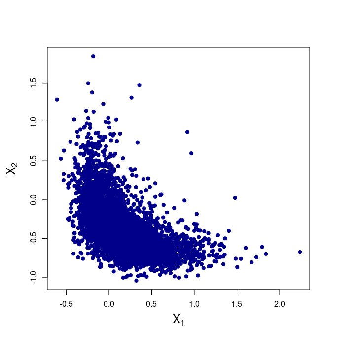
where ε∼𝒩⁡(0,σ2),σ2>0,\varepsilon\sim\mathcal{N}(0,\sigma^{2}),\penalty\ \sigma^{2}>0, is a gaussian noise. In our simulations we will take σ2=0.005.\sigma^{2}=0.005. Here, we choose the squared euclidian norm which has fourth moment under PP, defined by : ‖𝒙‖2=|x1|2+|x2|2\|\bm{x}\|^{2}=|x_{1}|^{2}+|x_{2}|^{2} (see Figure 3). Moreover, we consider dependent risk factors X1X_{1} and X2X_{2} via a bivariate Frank Copula with Gumbel marginals with parameter (μ,β)=(0,0.25)(\mu,\beta)=(0,0.25) and (−0.5,0.25)(-0.5,0.25) respectively (Figure 2).

Refer to caption
Figure 2: Sample of dependent Gumbel marginals via a Frank Copula.

Note that the above example satisfies the assumptions of Theorem 3.13.

Refer to caption
Figure 3: Monotonic function : R⁡(x1,x2)=|x1|2+|x2|2.R(x_{1},x_{2})=|x_{1}|^{2}+|x_{2}|^{2}.

Here we compare CCTE^M​H​D,αn1,n2\widehat{\CCTE}_{MHD,\alpha}^{n_{1},n_{2}} with the theoretical CCTEM​H​D,α\CCTE_{MHD,\alpha} for Mahalanobis depth. For the sake of simplicity, we take n1=n2=nn_{1}=n_{2}=n. Assuming that p,r≈+∞p,r\approx+\infty with our sample, we obtain that |CCTE^M​H​D,αn−CCTEM​H​D,α||\widehat{\CCTE}_{MHD,\alpha}^{n}-\CCTE_{MHD,\alpha}| decays to zero at most with a convergence rate o⁡(n).o(\sqrt{n}).

We provide a deterministic approximation of the true mean vector and covariance matrix, mm and Σ\Sigma respectively. However, due to the complexity of the level-sets as domains of integration in the computation of the CCTED\CCTE_{D}, we perform a Monte Carlo procedure to fix the "true" value of the CCTED\CCTE_{D} based on a sample of size 10810^{8} (without noise), that is:

∑i=1108R⁡(𝑿i)​𝟙𝑿i∈ℒM​H​D​(α)∑i=1108𝟙𝑿i∈ℒM​H​D​(α).\displaystyle\frac{\displaystyle\sum_{i=1}^{10^{8}}R(\bm{X}_{i})\mathds{1}_{\bm{X}_{i}\in\mathcal{L}_{MHD}(\alpha)}}{\displaystyle\sum_{i=1}^{10^{8}}\mathds{1}_{\bm{X}_{i}\in\mathcal{L}_{MHD}(\alpha)}}.

Recall that Theorem 3.13 illustrates convergence rates in probability, however, for the sake of computational simplicity, we provide 𝕃1\mathbb{L}^{1}-estimation for the CCTED\CCTE_{D} (which implies convergence results in probability). More precisely, we denote CCTE^αn¯:=CCTE^α,M​H​Dn¯\overline{\widehat{\CCTE}_{\alpha}^{n}}:=\overline{\widehat{\CCTE}_{\alpha,MHD}^{n}} the mean of the CCTE^M​H​D,αn\widehat{\CCTE}_{MHD,\alpha}^{n} based on 400400 simulations. The empirical standard deviation is

σ^=1399​∑j=1400(CCTE^α,jn−CCTE^αn¯)2,\hat{\sigma}=\displaystyle\sqrt{\frac{1}{399}\sum_{j=1}^{400}\left(\widehat{\CCTE}_{\alpha,j}^{n}-\overline{\widehat{\CCTE}_{\alpha}^{n}}\right)^{2}},

while the relative mean absolute error associated to CCTEαn^\widehat{\CCTE_{\alpha}^{n}}, denoted by RMAE, is defined as follows :

RMAE:=RMAEn,α=1400​∑j=1400|CCTE^α,jn−CCTEM​H​D,α(Y,𝑿))||CCTEM​H​D,α(Y,𝑿)|.\RMAE:={\RMAE}_{n,\alpha}=\displaystyle\frac{1}{400}\sum_{j=1}^{400}\frac{\big|\widehat{\CCTE}_{\alpha,j}^{n}-\CCTE_{MHD,\alpha}(Y,\bm{X}))\big|}{|\CCTE_{MHD,\alpha}(Y,\bm{X})|}.

Note that, most of the times, one uses the Relative Mean Squared Error (RMSE) rather than the RMAE. However, since our results are presented with absolute value (particularly Theorem 3.13), we work here with the RMAE for which we provide 𝕃1\mathbb{L}^{1}-estimation as well.

In Table 1, we provide the above estimations for different values of α\alpha and sample size nn.

nn α=0.1\alpha=0.1 α=0.2\alpha=0.2 α=0.5\alpha=0.5 α=0.8\alpha=0.8 α=0.9\alpha=0.9
CCTE=1.4237\CCTE=1.4237 CCTE=0.8831\CCTE=0.8831 CCTE=0.4804\CCTE=0.4804 CCTE=0.3831\CCTE=0.3831 CCTE=0.3661\CCTE=0.3661
100 Mean 1.2744 0.8568 0.4706 0.3806 0.3636
σ^\widehat{\sigma} 0.6596 0.2678 0.0716 0.045 0.042
RMAE 0.3733 0.2360 0.1217 0.0954 0.0933
1000 Mean 1.4125 0.8758 0.4801 0.3835 0.3664
σ^\widehat{\sigma} 0.1923 0.0782 0.0233 0.0153 0.0143
RMAE 0.1056 0.0696 0.0381 0.0318 0.0310
5000 Mean 1.4213 0.8808 0.4804 0.3832 0.3661
σ^\widehat{\sigma} 0.0855 0.0377 0.0106 0.0065 0.0061
RMAE 0.0476 0.0338 0.018 0.0138 0.0134
10000 Mean 1.4178 0.8807 0.4799 0.3828 0.3659
σ^\widehat{\sigma} 0.0625 0.0271 0.0071 0.0046 0.0043
RMAE 0.0361 0.0241 0.0117 0.0095 0.0094
50000 Mean 1.4231 0.8829 0.4807 0.3833 0.3663
σ^\widehat{\sigma} 0.0283 0.0118 0.0033 0.002 0.0019
RMAE 0.0158 0.0106 0.0055 0.0042 0.0041
Table 1: 𝕃1\mathbb{L}^{1}-estimation of CCTEα,M​H​D(𝐗,Y)\CCTE_{\alpha,MHD}(\mathbf{X},Y) and associated RMAE\RMAE for bivariate Frank Copulas with Gumbel marginals.

According to the results in Table 1, we observe that the error RMAEn\RMAE_{n} decreases as the sample size nn increases, as one may expect. Besides, remark that for low levels α\alpha (α=0.1\alpha=0.1) and sample sizes nn (n=100,1000n=100,1000), the value of RMAE\RMAE is relatively high. This may be explained by the fact that, for small values of α\alpha, there is fewer data to observe so that it becomes more difficult to estimate the mean CCTE^\widehat{\CCTE} as well as the α\alpha-level set. Indeed, for low levels α\alpha, the constant A=2/m∇A=2/m_{\nabla} is large since m∇m_{\nabla} approaches zero (see the proof of Proposition 3.5 and Theorem 3.6 in Section 5), meaning that the constant bounding the error (RMAE\RMAE) becomes large.

In Table 2, we also provide 𝕃1\mathbb{L}^{1}-convergence rates : Vn,α,δ=vn​(δ)⋅RMAEn,α,V_{n,\alpha,\delta}=v_{n}(\delta)\cdot\RMAE_{n,\alpha}, with vn​(δ)=n12−δv_{n}(\delta)=n^{\frac{1}{2}-\delta} for different values of δ\delta (see Figure 4).

α\alpha 100 1000 5000 10000 50000
0.1 0.05 2.9656 2.3641 2.1971 2.2773 2.0529
0.01 3.5654 3.1164 3.0889 3.2916 3.1646
0 3.7335 3.3393 3.3635 3.6092 3.5262
-0.01 3.9094 3.5782 3.6625 3.9574 3.9292
0.2 0.05 1.8749 1.5589 1.5602 1.5217 1.3821
0.01 2.2542 2.0551 2.1935 2.1996 2.1305
0 2.3604 2.2021 2.3885 2.4118 2.374
-0.01 2.4716 2.3595 2.6009 2.6445 2.6452
0.5 0.05 0.9666 0.8522 0.8298 0.7407 0.7124
0.01 1.1411 1.1234 1.1666 1.0707 1.0982
0 1.2169 1.2038 1.2703 1.1740 1.2236
-0.01 1.2742 1.2899 1.3832 1.2872 1.3635
0.8 0.05 0.7577 0.7119 0.6362 0.5989 0.5481
0.01 0.9111 0.9385 0.8945 0.8656 0.845
0 0.9539 1.0056 0.9740 0.9491 0.9415
-0.01 0.9988 1.0775 1.0606 1.0407 1.0491
0.9 0.05 0.7415 0.6949 0.6200 0.5952 0.5281
0.01 0.8914 0.9160 0.8717 0.8603 0.8141
0 0.9334 0.9815 0.9492 0.9433 0.9072
-0.01 0.9774 1.0517 1.0335 1.0344 1.0108
Table 2: Estimated n12−δ⋅RMAEn,αn^{\frac{1}{2}-\delta}\cdot\RMAE_{n,\alpha} based on M​H​DMHD for bivariate Frank Copulas with Gumbel marginals.
Refer to caption
Figure 4: Estimation of the convergence rates Vn,α,δV_{n,\alpha,\delta} associated to RMAE, based on M​H​DMHD for bivariate Frank Copulas with Gumbel marginals.

In Table 2 and Figure 4, the parameter δ\delta allows us to check that the critical regime is δ=0\delta=0 which corresponds to the n1/2n^{1/2}-convergence rate associated to the RMAE\RMAE.

5 Proofs of Section 3

Proofs of Section 3.1.

Proof of Theorem 3.2.

We can write

|CCTE^D,αn1,n2​(Y,𝑿)−CCTED,α(Y,𝑿)|⋅𝟙PS~n1​[ℒn1​(α)]>0\displaystyle\big|\widehat{\CCTE}_{D,\alpha}^{n_{1},n_{2}}(Y,\bm{X})-{\CCTE}_{D,\alpha}(Y,\bm{X})\big|\cdot\mathds{1}_{P_{\tilde{S}_{n_{1}}}[\mathcal{L}_{n_{1}}(\alpha)]>0}
=|1n2​∑i=1n2Yi​𝟙𝑿i∈ℒn1​(α)1n2​∑i=1n2𝟙𝑿i∈ℒn1​(α)−𝔼⁡[Y|𝑿∈ℒD​(α)]|⋅𝟙PS~n1​[ℒn1​(α)]>0\displaystyle=\displaystyle\left|\frac{\frac{1}{n_{2}}\sum_{i=1}^{n_{2}}Y_{i}\mathds{1}_{\bm{X}_{i}\in\mathcal{L}_{n_{1}}(\alpha)}}{\frac{1}{n_{2}}\sum_{i=1}^{n_{2}}\mathds{1}_{\bm{X}_{i}\in\mathcal{L}_{n_{1}}(\alpha)}}-\mathbb{E}[Y|\bm{X}\in\mathcal{L}_{D}(\alpha)]\right|\cdot\mathds{1}_{P_{\tilde{S}_{n_{1}}}[\mathcal{L}_{n_{1}}(\alpha)]>0}
≤|1n2​∑i=1n2Yi​𝟙𝑿i∈ℒn1​(α)1n2​∑i=1n2𝟙𝑿i∈ℒn1​(α)−𝔼S~n1​[Y|𝑿∈ℒn1​(α)]|⋅𝟙PS~n1​[ℒn1​(α)]>0\displaystyle\leq\displaystyle\left|\frac{\frac{1}{n_{2}}\sum_{i=1}^{n_{2}}Y_{i}\mathds{1}_{\bm{X}_{i}\in\mathcal{L}_{n_{1}}(\alpha)}}{\frac{1}{n_{2}}\sum_{i=1}^{n_{2}}\mathds{1}_{\bm{X}_{i}\in\mathcal{L}_{n_{1}}(\alpha)}}-\mathbb{E}_{\tilde{S}_{n_{1}}}[Y|\bm{X}\in\mathcal{L}_{n_{1}}(\alpha)]\right|\cdot\mathds{1}_{P_{\tilde{S}_{n_{1}}}[\mathcal{L}_{n_{1}}(\alpha)]>0}
+|𝔼S~n1[Y|𝑿∈ℒn1(α)]−𝔼[Y|𝑿∈ℒD(α)]|⋅𝟙PS~n1​[ℒn1​(α)]>0.\displaystyle\penalty\ \penalty\ +\displaystyle\left|\mathbb{E}_{\tilde{S}_{n_{1}}}[Y|\bm{X}\in\mathcal{L}_{n_{1}}(\alpha)]-\mathbb{E}[Y|\bm{X}\in\mathcal{L}_{D}(\alpha)]\right|\cdot\mathds{1}_{P_{\tilde{S}_{n_{1}}}[\mathcal{L}_{n_{1}}(\alpha)]>0}.

The proof of Theorem 3.2 is a modified version of the proof of Theorem 5.1 in Di Bernardino et al., 2015. The latter focuses on distribution functions instead of depth functions. Besides, in the proof of Theorem 3.2, we show that 𝟙PS~n1​[ℒn1​(α)]>0\mathds{1}_{P_{\tilde{S}_{n_{1}}}[\mathcal{L}_{n_{1}}(\alpha)]>0} converges to one in probability.

First recall that, in the following, probability measures involving events which depend on ℒn1​(α)\mathcal{L}_{n_{1}}(\alpha) are conditional expectations to the sample S~n1\tilde{S}_{n_{1}}. For notational convenience, we recall that

PS~n1[ℒn1(α)]:=ℙ[𝑿∈ℒn1(α)]P_{\tilde{S}_{n_{1}}}[\mathcal{L}_{n_{1}}(\alpha)]:=\mathbb{P}[\bm{X}\in\mathcal{L}_{n_{1}}(\alpha)]

which is a random variable. Moreover, note that the convergence to zero in probability implies directly the 𝒪P​(1)\mathcal{O}_{P}(1) result.

The proof of Theorem 3.2 is based on the two following preliminary results, Lemma 5.1 and Lemma 5.2. ∎

Lemma 5.1.

Under assumptions of Theorem 3.2, it holds that

|𝔼S~n1​[Y|𝑿∈ℒn1​(α)]−𝔼⁡[Y|𝑿∈ℒD​(α)]|=𝒪P,n1​(vn1−(1−1r)).\left|\mathbb{E}_{\tilde{S}_{n_{1}}}[Y|\bm{X}\in\mathcal{L}_{n_{1}}(\alpha)]-\mathbb{E}[Y|\bm{X}\in\mathcal{L}_{D}(\alpha)]\right|=\mathcal{O}_{P,n_{1}}\left(v_{n_{1}}^{-\left(1-\frac{1}{r}\right)}\right).
Proof of Lemma 5.1.

On the event {PS~n1[ℒn1(α)]>0}\left\{P_{\tilde{S}_{n_{1}}}[\mathcal{L}_{n_{1}}(\alpha)]>0\right\}, it holds

vn11−1r​|𝔼S~n1​[Y|𝑿∈ℒn1​(α)]−𝔼⁡[Y|𝑿∈ℒD​(α)]|=vn11−1r​|𝔼S~n1​[Y​𝟙𝑿∈ℒn1​(α)]PS~n1​[ℒn1​(α)]−𝔼⁡[Y​𝟙𝑿∈ℒD​(α)]P​[ℒD​(α)]|≤vn11−1rPS~n1​[ℒn1​(α)]​P​[ℒD​(α)]×(CLOSEP⁡[ℒD​(α)]​|𝔼S~n1​[Y​𝟙𝑿∈ℒn1​(α)]−𝔼⁡[Y​𝟙𝑿∈ℒD​(α)]|OPEN+|P⁡[ℒD​(α)]−PS~n1​[ℒn1​(α)]|​|𝔼⁡[Y​𝟙𝑿∈ℒD​(α)]|)≤vn11−1rPS~n1​[ℒn1​(α)]​P​[ℒD​(α)]×(|𝔼S~n1​[Y​𝟙𝑿∈ℒn1​(α)]−𝔼⁡[Y​𝟙𝑿∈ℒD​(α)]|CLOSEOPEN+𝔼⁡[|Y|]​|P⁡[ℒD​(α)]−PS~n1​[ℒn1​(α)]|).v_{n_{1}}^{1-\frac{1}{r}}\displaystyle\left|\mathbb{E}_{\tilde{S}_{n_{1}}}[Y|\bm{X}\in\mathcal{L}_{n_{1}}(\alpha)]-\mathbb{E}[Y|\bm{X}\in\mathcal{L}_{D}(\alpha)]\right|\\ =v_{n_{1}}^{1-\frac{1}{r}}\left|\displaystyle\frac{\mathbb{E}_{\tilde{S}_{n_{1}}}[Y\mathds{1}_{\bm{X}\in\mathcal{L}_{n_{1}}(\alpha)}]}{P_{\tilde{S}_{n_{1}}}[\mathcal{L}_{n_{1}}(\alpha)]}-\frac{\mathbb{E}[Y\mathds{1}_{\bm{X}\in\mathcal{L}_{D}(\alpha)}]}{P[\mathcal{L}_{D}(\alpha)]}\right|\hskip 142.26378pt\\ \leq\displaystyle\frac{v_{n_{1}}^{1-\frac{1}{r}}}{P_{\tilde{S}_{n_{1}}}[\mathcal{L}_{n_{1}}(\alpha)]P[\mathcal{L}_{D}(\alpha)]}\times\bigg(\hskip 213.39566pt\\ P[\mathcal{L}_{D}(\alpha)]\Big|\mathbb{E}_{\tilde{S}_{n_{1}}}[Y\mathds{1}_{\bm{X}\in\mathcal{L}_{n_{1}}(\alpha)}]-\mathbb{E}[Y\mathds{1}_{\bm{X}\in\mathcal{L}_{D}(\alpha)}]\Big|\\ +\displaystyle\left|P[\mathcal{L}_{D}(\alpha)]-P_{\tilde{S}_{n_{1}}}[\mathcal{L}_{n_{1}}(\alpha)]\right|\left|\mathbb{E}[Y\mathds{1}_{\bm{X}\in\mathcal{L}_{D}(\alpha)}]\right|\bigg)\\ \leq\displaystyle\frac{v_{n_{1}}^{1-\frac{1}{r}}}{P_{\tilde{S}_{n_{1}}}[\mathcal{L}_{n_{1}}(\alpha)]P[\mathcal{L}_{D}(\alpha)]}\times\bigg(\Big|\mathbb{E}_{\tilde{S}_{n_{1}}}[Y\mathds{1}_{\bm{X}\in\mathcal{L}_{n_{1}}(\alpha)}]-\mathbb{E}[Y\mathds{1}_{\bm{X}\in\mathcal{L}_{D}(\alpha)}]\Big|\hskip 28.45274pt\\ +\displaystyle\mathbb{E}[|Y|]\Big|P[\mathcal{L}_{D}(\alpha)]-P_{\tilde{S}_{n_{1}}}[\mathcal{L}_{n_{1}}(\alpha)]\Big|\bigg).\hskip 28.45274pt

Under Assumption (H0) and since vn1−1→0v_{n_{1}}^{-1}\to 0 as n1→∞n_{1}\to\infty, it holds that

PS~n1​[ℒn1​(α)​Δ​ℒD​(α)]→n1→∞ℙ0,P_{\tilde{S}_{n_{1}}}[\mathcal{L}_{n_{1}}(\alpha)\Delta\mathcal{L}_{D}(\alpha)]\xrightarrow[n_{1}\to\infty]{\mathbb{P}}0,

so that

PS~n1​[ℒn1​(α)]→n1→∞ℙP⁡[ℒD​(α)]>0,P_{\tilde{S}_{n_{1}}}[\mathcal{L}_{n_{1}}(\alpha)]\xrightarrow[n_{1}\to\infty]{\mathbb{P}}P[\mathcal{L}_{D}(\alpha)]>0,

and

ℙ[{PS~n1[ℒn1(α)]>0}]→n1→∞1.\mathbb{P}\left[\left\{P_{\tilde{S}_{n_{1}}}[\mathcal{L}_{n_{1}}(\alpha)]>0\right\}\right]\xrightarrow[n_{1}\to\infty]{}1. (5.1)

On the one hand,

vn11−1r​|PS~n1​[ℒn1​(α)]−P⁡[ℒD​(α)]|≤vn11−1r​PS~n1​[ℒD​(α)​Δ​ℒn1​(α)],\displaystyle v_{n_{1}}^{1-\frac{1}{r}}\left|P_{\tilde{S}_{n_{1}}}[\mathcal{L}_{n_{1}}(\alpha)]-P[\mathcal{L}_{D}(\alpha)]\right|\leq v_{n_{1}}^{1-\frac{1}{r}}P_{\tilde{S}_{n_{1}}}[\mathcal{L}_{D}(\alpha)\Delta\mathcal{L}_{n_{1}}(\alpha)],

so we obtain

vn11−1r​|PS~n1​[ℒn1​(α)]−P⁡[ℒD​(α)]|→n1→∞ℙ0.v_{n_{1}}^{1-\frac{1}{r}}\left|P_{\tilde{S}_{n_{1}}}[\mathcal{L}_{n_{1}}(\alpha)]-P[\mathcal{L}_{D}(\alpha)]\right|\xrightarrow[n_{1}\to\infty]{\mathbb{P}}0. (5.2)

On the other hand, using Hölder inequality

vn11−1r|𝔼S~n1​[Y​𝟙𝑿∈ℒn​(α)]\displaystyle v_{n_{1}}^{1-\frac{1}{r}}\big|\mathbb{E}_{\tilde{S}_{n_{1}}}[Y\mathds{1}_{\bm{X}\in\mathcal{L}_{n}(\alpha)}] −𝔼[Y𝟙𝑿∈ℒD​(α)]|\displaystyle-\mathbb{E}[Y\mathds{1}_{\bm{X}\in\mathcal{L}_{D}(\alpha)}]\big|
≤\displaystyle\leq vn11−1r​𝔼S~n1​[|Y|​𝟙𝑿∈ℒn1​(α)​Δ​ℒD​(α)]\displaystyle v_{n_{1}}^{1-\frac{1}{r}}\mathbb{E}_{\tilde{S}_{n_{1}}}\big[|Y|\mathds{1}_{\bm{X}\in\mathcal{L}_{n_{1}}(\alpha)\Delta\mathcal{L}_{D}(\alpha)}\big]
≤\displaystyle\leq vn11−1r​𝔼​[|Y|r]1r​𝔼S~n1​[𝟙𝑿∈ℒn1​(α)​Δ​ℒD​(α)]1−1r\displaystyle v_{n_{1}}^{1-\frac{1}{r}}\mathbb{E}\big[|Y|^{r}\big]^{\frac{1}{r}}\mathbb{E}_{\tilde{S}_{n_{1}}}\big[\mathds{1}_{\bm{X}\in\mathcal{L}_{n_{1}}(\alpha)\Delta\mathcal{L}_{D}(\alpha)}\big]^{1-\frac{1}{r}}
=\displaystyle= vn11−1r​PS~n1​[ℒn1​(α)​Δ​ℒD​(α)]1−1r​‖Y‖𝕃r​(Ω).\displaystyle v_{n_{1}}^{1-\frac{1}{r}}P_{\tilde{S}_{n_{1}}}[\mathcal{L}_{n_{1}}(\alpha)\Delta\mathcal{L}_{D}(\alpha)]^{1-\frac{1}{r}}\|Y\|_{\mathbb{L}^{r}(\Omega)}.

Since vn1​PS~n1​[ℒn1​(α)​Δ​ℒD​(α)]=𝒪P,n1​(1)v_{n_{1}}P_{\tilde{S}_{n_{1}}}[\mathcal{L}_{n_{1}}(\alpha)\Delta\mathcal{L}_{D}(\alpha)]=\mathcal{O}_{P,n_{1}}(1), it holds

vn11−1r​|𝔼S~n1​[Y​𝟙ℒn1​(α)]−𝔼⁡[Y​𝟙ℒD​(α)]|=𝒪P,n1​(1).v_{n_{1}}^{1-\frac{1}{r}}\big|\mathbb{E}_{\tilde{S}_{n_{1}}}[Y\mathds{1}_{\mathcal{L}_{n_{1}}(\alpha)}]-\mathbb{E}[Y\mathds{1}_{\mathcal{L}_{D}(\alpha)}]\big|=\mathcal{O}_{P,n_{1}}(1). (5.3)

Since the convergence to zero in probability implies the 𝒪P​(1)\mathcal{O}_{P}(1) result, the lemma follows directly from (5.1, (5.2), and (5.3). The case r=+∞r=+\infty is analogous.
∎

Lemma 5.2.

Under assumptions of Theorem 3.2, we obtain

|1n2​∑i=1n2Yi​𝟙𝑿i∈ℒn1​(α)1n2​∑i=1n2𝟙𝑿i∈ℒn1​(α)−𝔼⁡[Y|𝑿∈ℒn1​(α)]|=𝒪P,n1,n2​(n2−12).\displaystyle\left|\frac{\frac{1}{n_{2}}\sum_{i=1}^{n_{2}}Y_{i}\mathds{1}_{\bm{X}_{i}\in\mathcal{L}_{n_{1}}(\alpha)}}{\frac{1}{n_{2}}\sum_{i=1}^{n_{2}}\mathds{1}_{\bm{X}_{i}\in\mathcal{L}_{n_{1}}(\alpha)}}-\mathbb{E}[Y|\bm{X}\in\mathcal{L}_{n_{1}}(\alpha)]\right|=\mathcal{O}_{P,n_{1},n_{2}}(n_{2}^{-\frac{1}{2}}).
Proof of Lemma 5.2.

First, we distinguish the event in which
1n2​∑i=1n2𝟙𝑿i∈ℒn1​(α)=0\frac{1}{n_{2}}\sum_{i=1}^{n_{2}}\mathds{1}_{\bm{X}_{i}\in\mathcal{L}_{n_{1}}(\alpha)}=0, then the one in which 1n2​∑i=1n2𝟙𝑿i∈ℒn1​(α)≠0.\frac{1}{n_{2}}\sum_{i=1}^{n_{2}}\mathds{1}_{\bm{X}_{i}\in\mathcal{L}_{n_{1}}(\alpha)}\neq 0.
Let 0<ε<P⁡[ℒD​(α)].0<\varepsilon<P[\mathcal{L}_{D}(\alpha)]. Since the (Yi,𝑿i)1≤i≤n2(Y_{i},\bm{X}_{i})_{1\leq i\leq n_{2}} are iid so that the (𝑿i)1≤i≤n2(\bm{X}_{i})_{1\leq i\leq n_{2}} are iid, it holds that

ℙ\displaystyle\mathbb{P} [1n2∑i=1n2𝟙𝑿i∈ℒn1​(α)=0]\displaystyle\left[\frac{1}{n_{2}}\sum_{i=1}^{n_{2}}\mathds{1}_{\bm{X}_{i}\in\mathcal{L}_{n_{1}}(\alpha)}=0\right]
=𝔼[PS~n1[1n2∑i=1n2𝟙𝑿i∈ℒn1​(α)=0]]\displaystyle=\mathbb{E}\left[P_{\tilde{S}_{n_{1}}}\left[\frac{1}{n_{2}}\sum_{i=1}^{n_{2}}\mathds{1}_{\bm{X}_{i}\in\mathcal{L}_{n_{1}}(\alpha)}=0\right]\right]
=𝔼[∏i=1n2PS~n1[𝑿i∉ℒn1(α)]]\displaystyle=\mathbb{E}\left[\prod_{i=1}^{n_{2}}P_{\tilde{S}_{n_{1}}}\left[\bm{X}_{i}\notin\mathcal{L}_{n_{1}}(\alpha)\right]\right]
=𝔼[PS~n1[𝑿∉ℒn1(α)]n2]\displaystyle=\mathbb{E}\left[P_{\tilde{S}_{n_{1}}}\left[\bm{X}\notin\mathcal{L}_{n_{1}}(\alpha)\right]^{n_{2}}\right]
=𝔼⁡[(1−PS~n1​[ℒn1​(α)])n2​𝟙PS~n1​[ℒn1​(α)]≥ε]\displaystyle=\mathbb{E}\left[(1-P_{\tilde{S}_{n_{1}}}[\mathcal{L}_{n_{1}}(\alpha)])^{n_{2}}\mathds{1}_{P_{\tilde{S}_{n_{1}}}[\mathcal{L}_{n_{1}}(\alpha)]\geq\varepsilon}\right]
+𝔼⁡[(1−PS~n1​[ℒn1​(α)])n2​𝟙PS~n1​[ℒn1​(α)]<ε]\displaystyle\hskip 113.81102pt+\mathbb{E}\left[(1-P_{\tilde{S}_{n_{1}}}[\mathcal{L}_{n_{1}}(\alpha)])^{n_{2}}\mathds{1}_{P_{\tilde{S}_{n_{1}}}[\mathcal{L}_{n_{1}}(\alpha)]<\varepsilon}\right]
≤(1−ε)n2+ℙ[PS~n1[ℒn1(α)]<ε].\displaystyle\leq(1-\varepsilon)^{n_{2}}+\mathbb{P}\left[P_{\tilde{S}_{n_{1}}}[\mathcal{L}_{n_{1}}(\alpha)]<\varepsilon\right].

Since ε∈(0,P⁡[ℒD​(α)])\varepsilon\in\left(0,P[\mathcal{L}_{D}(\alpha)]\right) and PS~n1​[ℒn1​(α)]→n1→∞ℙP⁡[ℒD​(α)]P_{\tilde{S}_{n_{1}}}[\mathcal{L}_{n_{1}}(\alpha)]\xrightarrow[n_{1}\to\infty]{\mathbb{P}}P[\mathcal{L}_{D}(\alpha)] (see Lemma 5.1), we obtain ℙ[1n2∑i=1n2𝟙𝑿i∈ℒn1​(α)=0]→n1,n2→∞0.\mathbb{P}\left[\frac{1}{n_{2}}\sum_{i=1}^{n_{2}}\mathds{1}_{\bm{X}_{i}\in\mathcal{L}_{n_{1}}(\alpha)}=0\right]\xrightarrow[n_{1},n_{2}\to\infty]{}0. Now on the event
{1n2∑i=1n2𝟙𝑿i∈ℒn1​(α)≠0}∩{PS~n1[ℒn1(α)]>0}\left\{\frac{1}{n_{2}}\sum_{i=1}^{n_{2}}\mathds{1}_{\bm{X}_{i}\in\mathcal{L}_{n_{1}}(\alpha)}\neq 0\right\}\cap\left\{P_{\tilde{S}_{n_{1}}}[\mathcal{L}_{n_{1}}(\alpha)]>0\right\}, we can write

|\displaystyle\Bigg| 1n2​∑i=1n2Yi​𝟙𝑿i∈ℒn1​(α)1n2​∑i=1n2𝟙𝑿i∈ℒn1​(α)−𝔼S~n1[Y|𝑿∈ℒn1(α)]|\displaystyle\frac{\frac{1}{n_{2}}\sum_{i=1}^{n_{2}}Y_{i}\mathds{1}_{\bm{X}_{i}\in\mathcal{L}_{n_{1}}(\alpha)}}{\frac{1}{n_{2}}\sum_{i=1}^{n_{2}}\mathds{1}_{\bm{X}_{i}\in\mathcal{L}_{n_{1}}(\alpha)}}-\mathbb{E}_{\tilde{S}_{n_{1}}}[Y|\bm{X}\in\mathcal{L}_{n_{1}}(\alpha)]\Bigg|
=\displaystyle= |∑i=1n2Yi​𝟙𝑿i∈ℒn1​(α)∑i=1n2𝟙𝑿i∈ℒn1​(α)−𝔼S~n1​[Y​𝟙𝑿∈ℒn1​(α)]PS~n1​[ℒn1​(α)]|\displaystyle\left|\frac{\sum_{i=1}^{n_{2}}Y_{i}\mathds{1}_{\bm{X}_{i}\in\mathcal{L}_{n_{1}}(\alpha)}}{\sum_{i=1}^{n_{2}}\mathds{1}_{\bm{X}_{i}\in\mathcal{L}_{n_{1}}(\alpha)}}-\frac{\mathbb{E}_{\tilde{S}_{n_{1}}}[Y\mathds{1}_{\bm{X}\in\mathcal{L}_{n_{1}}(\alpha)}]}{P_{\tilde{S}_{n_{1}}}[\mathcal{L}_{n_{1}}(\alpha)]}\right|
≤\displaystyle\leq 11n2​∑i=1n2𝟙𝑿i∈ℒn1​(α)​|1n2​∑i=1n2Yi​𝟙𝑿i∈ℒn1​(α)−𝔼S~n1​[Y​𝟙𝑿∈ℒn1​(α)]|\displaystyle\frac{1}{\frac{1}{n_{2}}\sum_{i=1}^{n_{2}}\mathds{1}_{\bm{X}_{i}\in\mathcal{L}_{n_{1}}(\alpha)}}\bigg|\frac{1}{n_{2}}\sum_{i=1}^{n_{2}}Y_{i}\mathds{1}_{\bm{X}_{i}\in\mathcal{L}_{n_{1}}(\alpha)}-\mathbb{E}_{\tilde{S}_{n_{1}}}[Y\mathds{1}_{\bm{X}\in\mathcal{L}_{n_{1}}(\alpha)}]\bigg|
+|𝔼S~n1​[Y​𝟙𝑿∈ℒn1​(α)]|​|11n2​∑i=1n2𝟙𝑿i∈ℒn1​(α)−1PS~n1​[ℒn1​(α)]|\displaystyle+\big|\mathbb{E}_{\tilde{S}_{n_{1}}}[Y\mathds{1}_{\bm{X}\in\mathcal{L}_{n_{1}}(\alpha)}]\big|\bigg|\frac{1}{\frac{1}{n_{2}}\sum_{i=1}^{n_{2}}\mathds{1}_{\bm{X}_{i}\in\mathcal{L}_{n_{1}}(\alpha)}}-\frac{1}{P_{\tilde{S}_{n_{1}}}[\mathcal{L}_{n_{1}}(\alpha)]}\bigg|
≤\displaystyle\leq 11n2​∑i=1n2𝟙𝑿i∈ℒn1​(α)​|1n2​∑i=1n2Yi​𝟙𝑿i∈ℒn1​(α)−𝔼S~n1​[Y​𝟙𝑿∈ℒn1​(α)]|\displaystyle\frac{1}{\frac{1}{n_{2}}\sum_{i=1}^{n_{2}}\mathds{1}_{\bm{X}_{i}\in\mathcal{L}_{n_{1}}(\alpha)}}\bigg|\frac{1}{n_{2}}\sum_{i=1}^{n_{2}}Y_{i}\mathds{1}_{\bm{X}_{i}\in\mathcal{L}_{n_{1}}(\alpha)}-\mathbb{E}_{\tilde{S}_{n_{1}}}[Y\mathds{1}_{\bm{X}\in\mathcal{L}_{n_{1}}(\alpha)}]\bigg|
+𝔼⁡[|Y|]PS~n1​[ℒn1​(α)]​1n2​∑i=1n2𝟙𝑿i∈ℒn1​(α)​|1n2​∑i=1n2𝟙𝑿i∈ℒn1​(α)−PS~n1​[ℒn1​(α)]|.\displaystyle+\frac{\mathbb{E}[|Y|]}{P_{\tilde{S}_{n_{1}}}[\mathcal{L}_{n_{1}}(\alpha)]\frac{1}{n_{2}}\sum_{i=1}^{n_{2}}\mathds{1}_{\bm{X}_{i}\in\mathcal{L}_{n_{1}}(\alpha)}}\bigg|\frac{1}{n_{2}}\sum_{i=1}^{n_{2}}\mathds{1}_{\bm{X}_{i}\in\mathcal{L}_{n_{1}}(\alpha)}-P_{\tilde{S}_{n_{1}}}[\mathcal{L}_{n_{1}}(\alpha)]\bigg|. (R)

Let us first clarify the convergence of the denominator terms. Recall that under Assumption (H0) of Theorem 3.2,

PS~n1​[ℒn1​(α)]→n1→∞ℙP⁡[ℒD​(α)]>0,P_{\tilde{S}_{n_{1}}}[\mathcal{L}_{n_{1}}(\alpha)]\xrightarrow[n_{1}\to\infty]{\mathbb{P}}P[\mathcal{L}_{D}(\alpha)]>0,

and ℙ[{PS~n1[ℒn1(α)]>0}]→n1→∞1\mathbb{P}\left[\left\{P_{\tilde{S}_{n_{1}}}[\mathcal{L}_{n_{1}}(\alpha)]>0\right\}\right]\xrightarrow[n_{1}\to\infty]{}1 (see the proof of Lemma 5.1). Next, we prove

n212​(1n2​∑i=1n2𝟙𝑿i∈ℒn1​(α)−PS~n1​[ℒn1​(α)])=𝒪P,n1,n2​(1),n_{2}^{\frac{1}{2}}\left(\displaystyle\frac{1}{n_{2}}\sum_{i=1}^{n_{2}}\mathds{1}_{\bm{X}_{i}\in\mathcal{L}_{n_{1}}(\alpha)}-P_{\tilde{S}_{n_{1}}}[\mathcal{L}_{n_{1}}(\alpha)]\right)=\mathcal{O}_{P,n_{1},n_{2}}(1), (5.4)

so that we obtain

1n2​∑i=1n2𝟙𝑿i∈ℒn1​(α)−PS~n1​[ℒn1​(α)]→n1,n2→∞ℙ0,\displaystyle\frac{1}{n_{2}}\sum_{i=1}^{n_{2}}\mathds{1}_{\bm{X}_{i}\in\mathcal{L}_{n_{1}}(\alpha)}-P_{\tilde{S}_{n_{1}}}[\mathcal{L}_{n_{1}}(\alpha)]\xrightarrow[\begin{subarray}{c}n_{1},n_{2}\to\infty\end{subarray}]{\mathbb{P}}0, (5.5)

and

1n2​∑i=1n2𝟙𝑿i∈ℒn1​(α)→n1,n2→∞ℙP⁡[ℒD​(α)]>0.\frac{1}{n_{2}}\sum_{i=1}^{n_{2}}\mathds{1}_{\bm{X}_{i}\in\mathcal{L}_{n_{1}}(\alpha)}\xrightarrow[\begin{subarray}{c}n_{1},n_{2}\to\infty\end{subarray}]{\mathbb{P}}P[\mathcal{L}_{D}(\alpha)]>0.

Let us prove (5.4). Let n1≥1n_{1}\geq 1 and ε>0\varepsilon>0. Using Tchebychev inequality, we can write ℙ\mathbb{P}-a.s (here the event ω∈Ω\omega\in\Omega is one realisation of the sample S~n1\tilde{S}_{n_{1}} and is independent of ε\varepsilon)

PS~n1[|1n2∑i=1n2𝟙𝑿i∈ℒn1​(α)−PS~n1[ℒn1(α)]|≥ε]\displaystyle P_{\tilde{S}_{n_{1}}}\bigg[\Big|\displaystyle\frac{1}{n_{2}}\sum_{i=1}^{n_{2}}\mathds{1}_{\bm{X}_{i}\in\mathcal{L}_{n_{1}}(\alpha)}-P_{\tilde{S}_{n_{1}}}[\mathcal{L}_{n_{1}}(\alpha)]\Big|\geq\varepsilon\bigg] ≤𝕍S~n1​(1n2​∑i=1n2𝟙𝑿i∈ℒn1​(α))ε2\displaystyle\leq\displaystyle\frac{\mathbb{V}_{\tilde{S}_{n_{1}}}\big(\frac{1}{n_{2}}\sum_{i=1}^{n_{2}}\mathds{1}_{\bm{X}_{i}\in\mathcal{L}_{n_{1}}(\alpha)}\big)}{\varepsilon^{2}}
=𝕍S~n1​(𝟙𝑿1∈ℒn1​(α))n2​ε2\displaystyle=\displaystyle\frac{\mathbb{V}_{\tilde{S}_{n_{1}}}\big(\mathds{1}_{\bm{X}_{1}\in\mathcal{L}_{n_{1}}(\alpha)}\big)}{n_{2}\varepsilon^{2}}
≤1n2​ε2.\displaystyle\leq\frac{1}{n_{2}\varepsilon^{2}}.

Thus, taking Mε:=1/ε12M_{\varepsilon}:=1/\varepsilon^{\frac{1}{2}} it holds that

supn1,n2≥1ℙ[n212|1n2∑i=1n2𝟙𝑿i∈ℒn1​(α)−PS~n1[ℒn1(α)]|≥Mε]\displaystyle\sup_{n_{1},n_{2}\geq 1}\mathbb{P}\bigg[n_{2}^{\frac{1}{2}}\Big|\displaystyle\frac{1}{n_{2}}\sum_{i=1}^{n_{2}}\mathds{1}_{\bm{X}_{i}\in\mathcal{L}_{n_{1}}(\alpha)}-P_{\tilde{S}_{n_{1}}}[\mathcal{L}_{n_{1}}(\alpha)]\Big|\geq M_{\varepsilon}\bigg] ≤1n2​(Mεn212)2\displaystyle\leq\frac{1}{n_{2}\left(\frac{M_{\varepsilon}}{n_{2}^{\frac{1}{2}}}\right)^{2}}
=ε,\displaystyle=\varepsilon,

which means that (5.4) is satisfied. Similarly, we obtain

1n2​∑i=1n2Yi​𝟙𝑿i∈ℒn1​(α)−𝔼S~n1​[Y​𝟙𝑿∈ℒn1​(α)]=𝒪P,n1,n2​(n212)\frac{1}{n_{2}}\sum_{i=1}^{n_{2}}Y_{i}\mathds{1}_{\bm{X}_{i}\in\mathcal{L}_{n_{1}}(\alpha)}-\mathbb{E}_{\tilde{S}_{n_{1}}}[Y\mathds{1}_{\bm{X}\in\mathcal{L}_{n_{1}}(\alpha)}]=\mathcal{O}_{P,n_{1},n_{2}}\left(n_{2}^{\frac{1}{2}}\right)

Hence the result. ∎

Proofs of Section 3.2.

Remark 5.3.

Among the four properties of a depth function, the only necessary property in Proposition 3.5 is (D4) (vanishing at infinity). The latter guarantees that the set 𝒦ε​(α)\mathcal{K}_{\varepsilon}(\alpha) is compact in ℝd.\mathbb{R}^{d}. Indeed, as DD satisfies (D4), the assumption 0<ε<α0<\varepsilon<\alpha implies 𝒦ε​(α)\mathcal{K}_{\varepsilon}(\alpha) is bounded, moreover under (i), DD is continuous on 𝒦ε​(α)\mathcal{K}_{\varepsilon}(\alpha) so that 𝒦ε​(α)\mathcal{K}_{\varepsilon}(\alpha) is a closed set. By denoting (H​D)x(HD)_{x} the Hessian matrix of DD at x, one can note that MH:=supx∈𝒦ε​(α)‖|(H​D)x|‖<∞M_{H}:=\sup_{x\in\mathcal{K}_{\varepsilon}(\alpha)}{\left|\kern-1.07639pt\left|\kern-1.07639pt\left|(HD)_{x}\right|\kern-1.07639pt\right|\kern-1.07639pt\right|}<\infty, as a supremum of a continuous mapping on a compact set.

Proof of Proposition 3.5.

For the sake of simplicity, denote by [α±ε][\alpha\pm\varepsilon] the interval [α−ε,α+ε][\alpha-\varepsilon,\alpha+\varepsilon]. Under the assumptions of Proposition 3.5, Kε​(α):=D−1​([α±ε])K_{\varepsilon}(\alpha):=D^{-1}([\alpha\pm\varepsilon]) is compact and

MH:=supx∈Kε​(α)‖|H​Dx|‖<∞M_{H}:=\sup_{x\in K_{\varepsilon}(\alpha)}{\left|\kern-1.07639pt\left|\kern-1.07639pt\left|HD_{x}\right|\kern-1.07639pt\right|\kern-1.07639pt\right|}<\infty

(cf. Remark 5.3). We state the following useful lemma.

Lemma 5.4.

Under the assumptions of Proposition 3.5, there exist N:=Nε≥1N:=N_{\varepsilon}\geq 1, some points xi:=xi,ε∈𝒦ε2​(α)x_{i}:=x_{i,\varepsilon}\in\mathcal{K}_{\frac{\varepsilon}{2}}(\alpha), and some positive real numbers ri:=rxi∈ℝ+∗r_{i}:=r_{x_{i}}\in\mathbb{R}_{+}^{*}, 1≤i≤N1\leq i\leq N, s.t.

𝒦ε2​(α)⊂⋃i=1NB(xi,ri2)⊂⋃i=1NB(xi,ri)⊂𝒦ε​(α).\displaystyle\mathcal{K}_{\frac{\varepsilon}{2}}(\alpha)\subset\bigcup_{i=1}^{N}\Boule\bigg(x_{i},\frac{r_{i}}{2}\bigg)\subset\bigcup_{i=1}^{N}\Boule(x_{i},r_{i})\subset\mathcal{K}_{\varepsilon}(\alpha).

Proof of Lemma 5.4.

Since ε>0\varepsilon>0, then Kε2​(α)K_{\frac{\varepsilon}{2}}(\alpha) is a subset of the interior of 𝒦ε​(α)\mathcal{K}_{\varepsilon}(\alpha). Thus, for any x∈Kε2​(α)x\in K_{\frac{\varepsilon}{2}}(\alpha), there exists rx:=rx​(ε)>0r_{x}:=r_{x}(\varepsilon)>0 s.t.

B(x,rx)⊂𝒦ε​(α),\Boule(x,r_{x})\subset\mathcal{K}_{\varepsilon}(\alpha),

that is,

Kε2​(α)⊂⋃x∈Kε2​(α)B(x,rx2)⊂⋃x∈Kε2​(α)B(x,rx)⊂𝒦ε​(α).\displaystyle K_{\frac{\varepsilon}{2}}(\alpha)\subset\bigcup_{x\in K_{\frac{\varepsilon}{2}}(\alpha)}\Boule\bigg(x,\frac{r_{x}}{2}\bigg)\subset\bigcup_{x\in K_{\frac{\varepsilon}{2}}(\alpha)}\Boule(x,r_{x})\subset\mathcal{K}_{\varepsilon}(\alpha).

Since we have an open cover of the compact set Kε2​(α)\displaystyle K_{\frac{\varepsilon}{2}}(\alpha), then the latter has a finite cover. In other words, there exist N≥1N\geq 1, some points xi:=xi,ε∈𝒦ε2​(α)x_{i}:=x_{i,\varepsilon}\in\mathcal{K}_{\frac{\varepsilon}{2}}(\alpha), and ri:=rxi∈ℝ+∗r_{i}:=r_{x_{i}}\in\mathbb{R}_{+}^{*}, 1≤i≤N1\leq i\leq N, s.t.

𝒦ε2​(α)⊂⋃i=1NB(xi,ri2)⊂⋃i=1NB(xi,ri)⊂𝒦ε​(α).\displaystyle\mathcal{K}_{\frac{\varepsilon}{2}}(\alpha)\subset\bigcup_{i=1}^{N}\Boule\bigg(x_{i},\frac{r_{i}}{2}\bigg)\subset\bigcup_{i=1}^{N}\Boule(x_{i},r_{i})\subset\mathcal{K}_{\varepsilon}(\alpha).

Hence the result. ∎

Let 0<γ≤ε/20<\gamma\leq\varepsilon/2 and x∈𝒦γ​(α)x\in\mathcal{K}_{\gamma}(\alpha). For λ∈ℝ\lambda\in\mathbb{R}, define

yλ:=yλ,x=x+λ​(∇D)x‖(∇D)x‖,y_{\lambda}:=y_{\lambda,x}=x+\lambda\frac{(\nabla D)_{x}}{\|(\nabla D)_{x}\|},

with ‖(∇D)x‖≥m∇>0,\|(\nabla D)_{x}\|\geq m_{\nabla}>0, since 𝒦γ​(α)⊂𝒦ε​(α)\mathcal{K}_{\gamma}(\alpha)\subset\mathcal{K}_{\varepsilon}(\alpha). In what follows, we take

‖yλ−x‖=|λ|<min1≤i≤N⁡ri2.\|y_{\lambda}-x\|=|\lambda|<\displaystyle\min_{1\leq i\leq N}\frac{r_{i}}{2}.

It holds [yλ,x]⊂𝒦ε​(α)[y_{\lambda},x]\subset\mathcal{K}_{\varepsilon}(\alpha). Indeed, x∈𝒦γ​(α)x\in\mathcal{K}_{\gamma}(\alpha) so that Lemma 5.4 applies, namely, there exists 1≤i0≤N1\leq i_{0}\leq N s.t. x∈B(xi0,ri0/2),x\in\Boule(x_{i_{0}},r_{i_{0}}/2), and for all z∈[yλ,x],z\in[y_{\lambda},x],

‖z−xi0‖\displaystyle\|z-x_{i_{0}}\| ≤‖z−x‖+‖x−xi0‖\displaystyle\leq\|z-x\|+\|x-x_{i_{0}}\|
≤‖yλ−x‖+‖x−xi0‖\displaystyle\leq\|y_{\lambda}-x\|+\|x-x_{i_{0}}\|
=|λ|+‖x−xi0‖\displaystyle=|\lambda|+\|x-x_{i_{0}}\|
<min1≤i≤N⁡ri2+ri02\displaystyle<\min_{1\leq i\leq N}\frac{r_{i}}{2}+\frac{r_{i_{0}}}{2}
≤ri0.\displaystyle\leq r_{i_{0}}.

Thus, z∈B(xi0,ri0)⊂𝒦ε​(α)z\in\Boule(x_{i_{0}},r_{i_{0}})\subset\mathcal{K}_{\varepsilon}(\alpha) (cf. Lemma 5.4). Since |λ|<min1≤i≤N⁡ri/2\displaystyle|\lambda|<\min_{1\leq i\leq N}r_{i}/2, using a Taylor expansion on the line [x,yλ]⊂𝒦ε​(α)[x,y_{\lambda}]\subset\mathcal{K}_{\varepsilon}(\alpha), it holds

D⁡(yλ)=D⁡(x)+⟨(∇D)x,yλ−x⟩+12​⟨yλ−x,(H​D)x¯​(yλ−x)⟩,\displaystyle D(y_{\lambda})=D(x)+\langle(\nabla D)_{x},y_{\lambda}-x\rangle+\frac{1}{2}\left\langle y_{\lambda}-x,(HD)_{\overline{x}}(y_{\lambda}-x)\right\rangle, x¯∈[x,yλ],\overline{x}\in[x,y_{\lambda}],

then,

D⁡(yλ)=\displaystyle\displaystyle D(y_{\lambda})= D⁡(x)+λ​‖(∇D)x‖+λ22​‖(∇D)x‖2​⟨(∇D)x,(H​D)x¯​(∇D)x⟩.\displaystyle D(x)+\lambda\|(\nabla D)_{x}\|+\frac{\lambda^{2}}{2\|(\nabla D)_{x}\|^{2}}\left\langle(\nabla D)_{x},(HD)_{\overline{x}}(\nabla D)_{x}\right\rangle.

Using Cauchy-Schwarz inequality, it holds

|D⁡(yλ)−D⁡(x)−λ​‖(∇D)x‖|≤\displaystyle|D(y_{\lambda})-D(x)-\lambda\|(\nabla D)_{x}\||\leq\penalty\ λ22​‖(∇D)x‖2​‖(∇D)x‖​‖|(H​D)x¯|‖⋅‖(∇D)x‖\displaystyle\frac{\lambda^{2}}{2\|(\nabla D)_{x}\|^{2}}\|(\nabla D)_{x}\|{\left|\kern-1.07639pt\left|\kern-1.07639pt\left|(HD)_{\overline{x}}\right|\kern-1.07639pt\right|\kern-1.07639pt\right|}\cdot\|(\nabla D)_{x}\|
=\displaystyle= λ22​‖|(H​D)x¯|‖.\displaystyle\frac{\lambda^{2}}{2}{\left|\kern-1.07639pt\left|\kern-1.07639pt\left|(HD)_{\overline{x}}\right|\kern-1.07639pt\right|\kern-1.07639pt\right|}.

Since x¯∈𝒦ε​(α)\overline{x}\in\mathcal{K}_{\varepsilon}(\alpha), then ‖|(H​D)x¯|‖≤supx∈𝒦ε​(α)‖|(H​D)x¯|‖=MH<∞.{\left|\kern-1.07639pt\left|\kern-1.07639pt\left|(HD)_{\overline{x}}\right|\kern-1.07639pt\right|\kern-1.07639pt\right|}\leq\sup_{x\in\mathcal{K}_{\varepsilon}(\alpha)}{\left|\kern-1.07639pt\left|\kern-1.07639pt\left|(HD)_{\overline{x}}\right|\kern-1.07639pt\right|\kern-1.07639pt\right|}=M_{H}<\infty. For any |λ|<min1≤i≤N⁡ri/2\displaystyle|\lambda|<\min_{1\leq i\leq N}r_{i}/2, we obtain

D⁡(x)+λ​‖(∇D)x‖−λ22​MH≤D⁡(yλ)≤D⁡(x)+λ|(∇D)x|+λ22​MH.D(x)+\lambda\|(\nabla D)_{x}\|-\frac{\lambda^{2}}{2}M_{H}\leq D(y_{\lambda})\leq D(x)+\lambda\|(\nabla D)_{x}\|+\frac{\lambda^{2}}{2}M_{H}. (5.6)

If 0<λ<min1≤i≤N⁡ri/2\displaystyle 0<\lambda<\min_{1\leq i\leq N}r_{i}/2, then with the above inequality, we have

D⁡(yλ)≥D⁡(x)+λ​infx∈𝒦ε​(α)‖(∇D)x‖−λ22​MH=D⁡(x)+λ⁡(m∇−λ​MH2)\displaystyle D(y_{\lambda})\geq D(x)+\lambda\inf_{x\in\mathcal{K}_{\varepsilon}(\alpha)}\|(\nabla D)_{x}\|-\frac{\lambda^{2}}{2}M_{H}=D(x)+\lambda\left(m_{\nabla}-\lambda\frac{M_{H}}{2}\right) (5.7)

Suppose now MH>0M_{H}>0 (the case MH=0M_{H}=0 is trivial). That way, if 0<λ<m∇MH∧min1≤i≤N⁡ri/20<\lambda<\frac{m_{\nabla}}{M_{H}}\wedge\min_{1\leq i\leq N}r_{i}/2, using (5.7),

D⁡(yλ)≥D⁡(x)+λ​m∇2D(y_{\lambda})\geq D(x)+\lambda\frac{m_{\nabla}}{2}.

Similarly, using the right hand side of inequality (5.6), for any 0<λ<m∇MH∧min1≤i≤N⁡ri2\displaystyle 0<\lambda<\frac{m_{\nabla}}{M_{H}}\wedge\min_{1\leq i\leq N}\frac{r_{i}}{2},

D⁡(y−λ)≤D⁡(x)−λ​m∇2.D(y_{-\lambda})\leq D(x)-\lambda\frac{m_{\nabla}}{2}.

To sum up, for any 0<γ≤ε/20<\gamma\leq\varepsilon/2, x∈𝒦γ​(α)x\in\mathcal{K}_{\gamma}(\alpha) and 0<λ<m∇MH∧min1≤i≤N⁡ri2\displaystyle 0<\lambda<\frac{m_{\nabla}}{M_{H}}\wedge\min_{1\leq i\leq N}\frac{r_{i}}{2}, it holds

D⁡(yλ)≥D⁡(x)+λ​m∇2,\displaystyle D(y_{\lambda})\geq D(x)+\lambda\frac{m_{\nabla}}{2}, (5.8)
D⁡(y−λ)≤D⁡(x)−λ​m∇2.\displaystyle D(y_{-\lambda})\leq D(x)-\lambda\frac{m_{\nabla}}{2}. (5.9)

Choose γ:=[m∇4​(m∇MH∧min1≤i≤N⁡ri2)]∧ε2>0.\displaystyle\gamma:=\displaystyle\left[\frac{m_{\nabla}}{4}\left(\frac{m_{\nabla}}{M_{H}}\wedge\min_{1\leq i\leq N}\frac{r_{i}}{2}\right)\right]\wedge\frac{\varepsilon}{2}>0. Now we show :

if |α−β|≤γ|\alpha-\beta|\leq\gamma, then dH({D=α},{D=β})≤2m∇|α−β|d_{H}(\left\{D=\alpha\right\},\left\{D=\beta\right\})\leq\frac{2}{m_{\nabla}}|\alpha-\beta|.

Assume |α−β|≤γ|\alpha-\beta|\leq\gamma.
Let β\beta be s.t. 0<β−α≤γ0<\beta-\alpha\leq\gamma. In this case, β=α+η\beta=\alpha+\eta with 0<η≤γ.0<\eta\leq\gamma. First, we have to find an upper bound for supx∈{D=β}dist(x,{D=α})\sup_{x\in\left\{D=\beta\right\}}\dist(x,\left\{D=\alpha\right\}). Let x∈{D=β}x\in\left\{D=\beta\right\}, i.e. D⁡(x)=β=α+ηD(x)=\beta=\alpha+\eta. Since 0<η≤γ0<\eta\leq\gamma, 0<D⁡(x)−α≤γ,0<D(x)-\alpha\leq\gamma, i.e. x∈𝒦γ​(α)x\in\mathcal{K}_{\gamma}(\alpha). Choose λ:=2​ηm∇∈(0,m∇MH∧min1≤i≤N⁡ri2)\lambda:=\frac{2\eta}{m_{\nabla}}\in\displaystyle\left(0,\frac{m_{\nabla}}{M_{H}}\wedge\min_{1\leq i\leq N}\frac{r_{i}}{2}\right) so that with (5.9),

D⁡(y−λ)≤D⁡(x)−λ​m∇2=D⁡(x)−η=α<D⁡(x).D(y_{-\lambda})\leq D(x)-\lambda\frac{m_{\nabla}}{2}=D(x)-\eta=\alpha<D(x).

From the above inequality and the continuity property of z↦D⁡(z)z\mapsto D(z) on 𝒦ε​(α)⊃[y−λ,x]\mathcal{K}_{\varepsilon}(\alpha)\supset[y_{-\lambda},x], there exists a point y∈[y−λ,x]y\in[y_{-\lambda},x] s.t. D⁡(y)=αD(y)=\alpha. Moreover,

‖x−y‖≤‖x−y−λ‖=|λ|=2​ηm∇=2m∇​(β−α).\|x-y\|\leq\|x-y_{-\lambda}\|=|\lambda|=\frac{2\eta}{m_{\nabla}}=\frac{2}{m_{\nabla}}(\beta-\alpha).

As a consequence, for all x∈{D=β}x\in\left\{D=\beta\right\},

dist(x,{D=α}≤∥x−y∥≤2m∇|β−α|.\dist(x,\left\{D=\alpha\right\}\leq\|x-y\|\leq\frac{2}{m_{\nabla}}|\beta-\alpha|.

So

supx∈{D=β}dist(x,{D=α})≤2m∇|β−α|.\sup_{x\in\left\{D=\beta\right\}}\dist(x,\left\{D=\alpha\right\})\leq\frac{2}{m_{\nabla}}|\beta-\alpha|.

In order to get an upper bound for supx∈{D=α}dist(x,{D=β})\sup_{x\in\left\{D=\alpha\right\}}\dist(x,\left\{D=\beta\right\}), we use the inequality (5.8) by proceeding in a similar way.


The proof in the case 0>β−α>−γ0>\beta-\alpha>-\gamma is completely analogous. ∎

Proof of Theorem 3.6.

Let α∈(0,αmax​(P))\alpha\in(0,\alpha_{\max}(P)).


Step 1 : we need to find an upper bound for supx∈∂ℒ⁡(α)d⁡(x,∂ℒn​(α)).\sup_{x\in\partial\mathcal{L}(\alpha)}d(x,\partial\mathcal{L}_{n}(\alpha)).


Let x∈∂ℒ⁡(α)x\in\partial\mathcal{L}(\alpha). Denote εn=2​‖Dn−D‖∞\varepsilon_{n}=2\|D_{n}-D\|_{\infty}. Under the assumptions of Theorem 3.6 εn→0​ℙ\varepsilon_{n}\to 0\penalty\ \mathbb{P}-a.s, so that ℙ\mathbb{P}-a.s, there exists an integer n0:=n0​(ω)≥1n_{0}:=n_{0}(\omega)\geq 1 (independent from xx), s.t. for all n≥n0n\geq n_{0}, εn≤γ.\varepsilon_{n}\leq\gamma. Taking β=α+εn\beta=\alpha+\varepsilon_{n}, it holds

ℙ\mathbb{P}-a.s, for all n≥n0n\geq n_{0}, dH​(∂ℒ⁡(α+εn),∂ℒ⁡(α))≤A​εn.d_{H}(\partial\mathcal{L}(\alpha+\varepsilon_{n}),\partial\mathcal{L}(\alpha))\leq A\varepsilon_{n}.

Thus, from the above inequality and using the continuity property of DD, ℙ\mathbb{P}-a.s, for all n≥n0n\geq n_{0}, there exists un:=ux,εn∈∂ℒ⁡(α+εn)u_{n}:=u_{x,\varepsilon_{n}}\in\partial\mathcal{L}(\alpha+\varepsilon_{n}) i.e. D⁡(un)=α+εnD(u_{n})=\alpha+\varepsilon_{n}, and ln:=lx,εn∈∂ℒ⁡(α−εn)l_{n}:=l_{x,\varepsilon_{n}}\in\partial\mathcal{L}(\alpha-\varepsilon_{n}) i.e. D⁡(ln)=α−εn,D(l_{n})=\alpha-\varepsilon_{n}, s.t.

‖un−x‖≤A​εn​ and ​‖ln−x‖≤A​εn.\|u_{n}-x\|\leq A\varepsilon_{n}\text{\penalty\ and\penalty\ }\|l_{n}-x\|\leq A\varepsilon_{n}.

Let us assume ‖Dn−D‖∞>0\|D_{n}-D\|_{\infty}>0 (the case ‖Dn−D‖∞=0\|D_{n}-D\|_{\infty}=0 is trivial). In this case,

Dn​(un)=Dn​(un)+α+εn−D⁡(un)≥α+εn−‖Dn−D‖∞=α+‖Dn−D‖∞>α.D_{n}(u_{n})=D_{n}(u_{n})+\alpha+\varepsilon_{n}-D(u_{n})\geq\alpha+\varepsilon_{n}-\|D_{n}-D\|_{\infty}=\alpha+\|D_{n}-D\|_{\infty}>\alpha.

Similarly, we have Dn​(ln)<α.D_{n}(l_{n})<\alpha. So ℙ\mathbb{P}-a.s, for all n≥n0n\geq n_{0},

Dn​(ln)<α<Dn​(un).D_{n}(l_{n})<\alpha<D_{n}(u_{n}).

For the sake of simplicity, we denote here ℒn:={x:Dn​(x)≤α}\mathcal{L}_{n}:=\left\{x:D_{n}(x)\leq\alpha\right\}. Then, almost surely, for all n≥n0n\geq n_{0}, ℒn\mathcal{L}_{n} is non-empty (since it contains lnl_{n}). And by definition, ln∈ℒn⊂ℒn¯l_{n}\in\mathcal{L}_{n}\subset\overline{\mathcal{L}_{n}}. Denoting by ℒnc\mathcal{L}_{n}^{c} the complementary of ℒn\mathcal{L}_{n} in ℝd\mathbb{R}^{d}, it holds un∈ℒnc⊂ℒnc¯=(ℒn̊)c,u_{n}\in\mathcal{L}_{n}^{c}\subset\overline{\mathcal{L}_{n}^{c}}=(\mathring{\mathcal{L}_{n}})^{c}, that is, un∉ℒn̊u_{n}\notin\mathring{\mathcal{L}_{n}}. Then,

ℙ\mathbb{P}-a.s, for all n≥n0n\geq n_{0}, there exists zn∈[ln,un]∩∂ℒnz_{n}\in[l_{n},u_{n}]\cap\partial\mathcal{L}_{n}.

Thus, ℙ\mathbb{P}-a.s, for all n≥n0n\geq n_{0},

dist(x,∂ℒn​(α))\displaystyle\dist(x,\partial\mathcal{L}_{n}(\alpha)) ≤‖x−zn‖\displaystyle\leq\|x-z_{n}\|
≤‖x−un‖+‖un−zn‖\displaystyle\leq\|x-u_{n}\|+\|u_{n}-z_{n}\|
≤‖un−x‖+‖un−ln‖\displaystyle\leq\|u_{n}-x\|+\|u_{n}-l_{n}\|
≤‖un−x‖+‖un−x‖+‖x−ln‖\displaystyle\leq\|u_{n}-x\|+\|u_{n}-x\|+\|x-l_{n}\|
≤3​A​εn\displaystyle\leq 3A\varepsilon_{n}
=6​A​‖Dn−D‖∞.\displaystyle=6A\|D_{n}-D\|_{\infty}.

Since the previous inequality holds for all x∈∂ℒ⁡(α)x\in\partial\mathcal{L}(\alpha), we have, ℙ\mathbb{P}-a.s, for all n≥n0n\geq n_{0},

supx∈∂ℒ⁡(α)d⁡(x,∂ℒn​(α))≤6​A​‖Dn−D‖∞.\displaystyle\sup_{x\in\partial\mathcal{L}(\alpha)}d(x,\partial\mathcal{L}_{n}(\alpha))\leq 6A\|D_{n}-D\|_{\infty}.

Step 2 : Let us find an upper bound for supx∈∂ℒn​(α)d⁡(x,∂ℒ⁡(α)).\sup_{x\in\partial\mathcal{L}_{n}(\alpha)}d(x,\partial\mathcal{L}(\alpha)).


Let xn∈∂ℒn(α):=∂ℒn={Dn≤α}¯∩{Dn>α}¯⊂{Dn≥α}¯={Dn≥α}x_{n}\in\partial\mathcal{L}_{n}(\alpha):=\partial\mathcal{L}_{n}=\overline{\left\{D_{n}\leq\alpha\right\}}\cap\overline{\left\{D_{n}>\alpha\right\}}\subset\overline{\left\{D_{n}\geq\alpha\right\}}=\left\{D_{n}\geq\alpha\right\}, since DnD_{n} is a.s upper-semicontinuous, so that the upper level set based on DnD_{n} is closed. Then, Dn​(xn)≥αD_{n}(x_{n})\geq\alpha. Furthermore, since xn∈{Dn≤α}¯x_{n}\in\overline{\left\{D_{n}\leq\alpha\right\}}, there exists ℓn\ell_{n} "close" enough to xnx_{n} s.t. Dn​(ℓn)≤αD_{n}(\ell_{n})\leq\alpha, and s.t. by continuity of DD, |D⁡(xn)−D⁡(ℓn)|≤εn/2.|D(x_{n})-D(\ell_{n})|\leq\varepsilon_{n}/2. On the one hand,

D⁡(xn)=Dn​(xn)−Dn​(xn)+D⁡(xn)≥α−εn/2≥α−εn,D(x_{n})=D_{n}(x_{n})-D_{n}(x_{n})+D(x_{n})\geq\alpha-\varepsilon_{n}/2\geq\alpha-\varepsilon_{n},

on the other hand,

D⁡(xn)\displaystyle D(x_{n}) =Dn​(ℓn)−Dn​(ℓn)+D⁡(ℓn)−D⁡(ℓn)+D⁡(xn)\displaystyle=D_{n}(\ell_{n})-D_{n}(\ell_{n})+D(\ell_{n})-D(\ell_{n})+D(x_{n})
≤α+εn/2+εn/2,\displaystyle\leq\alpha+\varepsilon_{n}/2+\varepsilon_{n}/2,

so,

|D⁡(xn)−α|≤εn.|D(x_{n})-\alpha|\leq\varepsilon_{n}.

Recall that, a.s for all n≥n0n\geq n_{0}, εn≤γ.\varepsilon_{n}\leq\gamma. Then, using property (L) with β=D⁡(xn)\beta=D(x_{n}), we can write

dist(xn,∂ℒ⁡(α))≤dH​(∂ℒ⁡(D⁡(xn)),∂ℒ⁡(α))\displaystyle\dist(x_{n},\partial\mathcal{L}(\alpha))\leq d_{H}(\partial\mathcal{L}(D(x_{n})),\partial\mathcal{L}(\alpha)) ≤A​|D⁡(xn)−α|\displaystyle\leq A|D(x_{n})-\alpha|
≤2​A​‖Dn−D‖∞.\displaystyle\leq 2A\|D_{n}-D\|_{\infty}.

Now we deduce that, a.s. for nn large enough,

supx∈∂ℒn​(α)d⁡(x,∂ℒ⁡(α))≤2​A​‖Dn−D‖∞.\sup_{x\in\partial\mathcal{L}_{n}(\alpha)}d(x,\partial\mathcal{L}(\alpha))\leq 2A\|D_{n}-D\|_{\infty}.

Hence the result. ∎

Proofs of Section 3.3.

Proof of Proposition 3.11.

(i) The function M​H​D​(⋅)MHD(\cdot) is infinitely differentiable on ℝd\mathbb{R}^{d}, and denoting μ=μ𝑿\mu=\mu_{\bm{X}}, we can write for any 1≤k≤d1\leq k\leq d,

∂M​H​D​(x)∂xk\displaystyle\displaystyle\frac{\partial MHD(x)}{\partial x_{k}} =−M​H​D​(x)2​∂∂xk​[∑i,j=1d(xi−μi)​(Σ𝑿−1)i​j​(xj−μj)]\displaystyle=-MHD(x)^{2}\frac{\partial}{\partial x_{k}}\Bigg[\displaystyle\sum_{i,j=1}^{d}(x_{i}-\mu_{i})(\Sigma_{\bm{X}}^{-1})_{ij}(x_{j}-\mu_{j})\Bigg]
=−MHD(x)2⋅2[∑i=1d(Σ𝑿−1)k​i(xi−μi)], (Σ𝑿−1 is symmetric)\displaystyle=-MHD(x)^{2}\cdot 2\Bigg[\displaystyle\sum_{i=1}^{d}(\Sigma_{\bm{X}}^{-1})_{ki}(x_{i}-\mu_{i})\Bigg],\text{\penalty\ }(\Sigma_{\bm{X}}^{-1}\text{\penalty\ is symmetric})
=−2​M​H​D​(x)2​[Σ𝑿−1​(x−μ)]k.\displaystyle=-2MHD(x)^{2}\bigg[\Sigma_{\bm{X}}^{-1}(x-\mu)\bigg]_{k}.

So

(∇MHD)x=−2MHD(x)2Σ𝑿−1(x−μ).(\nabla MHD)_{x}=-2MHD(x)^{2}\Sigma_{\bm{X}}^{-1}(x-\mu).

Since M​H​D​(x)>0MHD(x)>0,

(∇MHD)x=0⟺x=μ=μ𝑿.(\nabla MHD)_{x}=0\Longleftrightarrow x=\mu=\mu_{\bm{X}}.

Thus,

∥(∇MHD)x∥>0,for all x≠μ𝑿.\displaystyle\|(\nabla MHD)_{x}\|>0,\penalty\ \text{for all\penalty\ }x\neq\mu_{\bm{X}}.

Now since x∈ℝd↦∥(∇MHD)x∥x\in\mathbb{R}^{d}\mapsto\|(\nabla MHD)_{x}\| is continuous and 𝒦ε​(α)\mathcal{K}_{\varepsilon}(\alpha) is compact, then there exists x0∈𝒦ε​(α)x_{0}\in\mathcal{K}_{\varepsilon}(\alpha) in which the infimum m∇m_{\nabla} is attained,

m∇=∥(∇MHD)x0∥>0.m_{\nabla}=\|(\nabla MHD)_{x_{0}}\|>0.

The latter inequality is strict since x0∈𝒦ε​(α)x_{0}\in\mathcal{K}_{\varepsilon}(\alpha), and μ𝑿∉𝒦ε​(α)\mu_{\bm{X}}\notin\mathcal{K}_{\varepsilon}(\alpha) (from the assumption OPENε<1−α).\varepsilon<1-\alpha). Indeed,

μ𝑿∈𝒦ε​(α)⇔|M​H​D​(μ𝑿)−α|≤ε⇔|1−α|=1−α≤ε.\mu_{\bm{X}}\in\mathcal{K}_{\varepsilon}(\alpha)\Leftrightarrow|MHD(\mu_{\bm{X}})-\alpha|\leq\varepsilon\Leftrightarrow|1-\alpha|=1-\alpha\leq\varepsilon.

(ii) It suffices to prove

‖M​H​Dn−M​H​D‖∞,ℝd→n→∞a.s0,\|MHD_{n}-MHD\|_{\infty,\mathbb{R}^{d}}\xrightarrow[n\to\infty]{a.s}0, (5.10)

by recalling that αmax​(P)=1\alpha_{\max}(P)=1 for M​H​DMHD depth. The result is hence a straight forward application of Proposition 3.5 and Theorem 3.6. In order to prove (5.10), one can refer to the computations in the proof of Theorem 3.12 and obtain the desired result knowing that Σ^n→n→∞a.sΣ,\hat{\Sigma}_{n}\xrightarrow[n\to\infty]{a.s}\Sigma, and μ^n→n→∞a.sμ.\hat{\mu}_{n}\xrightarrow[n\to\infty]{a.s}\mu. ∎

Proof of Theorem 3.12.

Let x∈ℝd.x\in\mathbb{R}^{d}. Denote μ:=μ𝑿\mu:=\mu_{\bm{X}} and Σ:=Σ𝑿\Sigma:=\Sigma_{\bm{X}}, we can write

|MHDn(x)−\displaystyle|MHD_{n}(x)- MHD(x)|\displaystyle MHD(x)|
=|11+t(x−μ^n)Σ^n−1(x−μ^n)−11+t(x−μ)Σ−1(x−μ)|\displaystyle=\displaystyle\left|\frac{1}{1+\penalty\ ^{t}(x-\hat{\mu}_{n})\hat{\Sigma}_{n}^{-1}(x-\hat{\mu}_{n})}-\frac{1}{1+\penalty\ ^{t}(x-\mu)\Sigma^{-1}(x-\mu)}\right|
≤|t(x−μ^n)Σ^n−1(x−μ^n)−t(x−μ)Σ−1(x−μ)|1+t(x−μ)Σ−1(x−μ).\displaystyle\leq\displaystyle\frac{\left|\penalty\ {}^{t}(x-\hat{\mu}_{n})\hat{\Sigma}_{n}^{-1}(x-\hat{\mu}_{n})-\penalty\ ^{t}(x-\mu)\Sigma^{-1}(x-\mu)\right|}{1+\penalty\ ^{t}(x-\mu)\Sigma^{-1}(x-\mu)}.

Since Σ\Sigma is a positive definite symmetric and invertible matrix, we can make the change of variable y=Σ−12​(x−μ)y=\Sigma^{-\frac{1}{2}}(x-\mu). So that,

∥MHDn\displaystyle\displaystyle\|MHD_{n} −MHD∥∞,ℝd≤supy∈ℝd|‖Σ^n−12​(Σ12​y+μ−μ^n)‖2−‖y‖2|1+‖y‖2.\displaystyle-MHD\|_{\infty,\mathbb{R}^{d}}\leq\displaystyle\sup_{y\in\mathbb{R}^{d}}\frac{\left|\|\hat{\Sigma}_{n}^{-\frac{1}{2}}(\Sigma^{\frac{1}{2}}y+\mu-\hat{\mu}_{n})\|^{2}-\penalty\ \|y\|^{2}\right|}{1+\|y\|^{2}}.

Now, denoting by IdI_{d} the identity matrix of size dd, and using a triangle inequality then Cauchy-Schwarz inequality, it holds

|‖Σ^n−12​(Σ12​y+μ−μ^n)‖2−‖y‖2|1+‖y‖2\displaystyle\frac{\left|\|\hat{\Sigma}_{n}^{-\frac{1}{2}}(\Sigma^{\frac{1}{2}}y+\mu-\hat{\mu}_{n})\|^{2}-\penalty\ \|y\|^{2}\right|}{1+\|y\|^{2}}
≤|‖Σ^n−12​Σ12​y‖2−‖y‖2|+‖Σ^n−12​(μ−μ^n)‖2+2​|⟨Σ^n−12​Σ12​y,Σ^n−12​(μ−μ^n)⟩|1+‖y‖2\displaystyle\leq\frac{\left|\|\hat{\Sigma}_{n}^{-\frac{1}{2}}\Sigma^{\frac{1}{2}}y\|^{2}-\penalty\ \|y\|^{2}\right|+\|\hat{\Sigma}_{n}^{-\frac{1}{2}}(\mu-\hat{\mu}_{n})\|^{2}+2\left|\left\langle\hat{\Sigma}_{n}^{-\frac{1}{2}}\Sigma^{\frac{1}{2}}y,\hat{\Sigma}_{n}^{-\frac{1}{2}}(\mu-\hat{\mu}_{n})\right\rangle\right|}{1+\|y\|^{2}}
≤‖|Σ12​Σ^n−1​Σ12−Id|‖​‖y‖2+‖Σ^n−12​(μ−μ^n)‖2+2​‖|Σ^n−1|‖​‖|Σ12|‖​‖y‖​‖μ−μ^n‖1+‖y‖2,\displaystyle\leq\frac{{\left|\kern-1.07639pt\left|\kern-1.07639pt\left|\Sigma^{\frac{1}{2}}\hat{\Sigma}_{n}^{-1}\Sigma^{\frac{1}{2}}-I_{d}\right|\kern-1.07639pt\right|\kern-1.07639pt\right|}\|y\|^{2}+\|\hat{\Sigma}_{n}^{-\frac{1}{2}}(\mu-\hat{\mu}_{n})\|^{2}+2{\left|\kern-1.07639pt\left|\kern-1.07639pt\left|\hat{\Sigma}_{n}^{-1}\right|\kern-1.07639pt\right|\kern-1.07639pt\right|}{\left|\kern-1.07639pt\left|\kern-1.07639pt\left|\Sigma^{\frac{1}{2}}\right|\kern-1.07639pt\right|\kern-1.07639pt\right|}\|y\|\|\mu-\hat{\mu}_{n}\|}{1+\|y\|^{2}},

This, together with the fact that 2​‖y‖/(1+‖y‖2)≤12\|y\|/(1+\|y\|^{2})\leq 1, for all y∈ℝdy\in\mathbb{R}^{d},

|‖Σ^n−12​(Σ12​y+μ−μ^n)‖2−‖y‖2|1+‖y‖2\displaystyle\frac{\left|\|\hat{\Sigma}_{n}^{-\frac{1}{2}}(\Sigma^{\frac{1}{2}}y+\mu-\hat{\mu}_{n})\|^{2}-\penalty\ \|y\|^{2}\right|}{1+\|y\|^{2}}
≤‖|Σ12​Σ^n−1​Σ12−Id|‖+‖Σ^n−12​(μ−μ^n)‖2+‖|Σ^n−1|‖⋅‖|Σ12|‖​‖μ−μ^n‖.\displaystyle\leq{\left|\kern-1.07639pt\left|\kern-1.07639pt\left|\Sigma^{\frac{1}{2}}\hat{\Sigma}_{n}^{-1}\Sigma^{\frac{1}{2}}-I_{d}\right|\kern-1.07639pt\right|\kern-1.07639pt\right|}+\|\hat{\Sigma}_{n}^{-\frac{1}{2}}(\mu-\hat{\mu}_{n})\|^{2}+{\left|\kern-1.07639pt\left|\kern-1.07639pt\left|\hat{\Sigma}_{n}^{-1}\right|\kern-1.07639pt\right|\kern-1.07639pt\right|}\cdot{\left|\kern-1.07639pt\left|\kern-1.07639pt\left|\Sigma^{\frac{1}{2}}\right|\kern-1.07639pt\right|\kern-1.07639pt\right|}\|\mu-\hat{\mu}_{n}\|.

Now since the right hand side of the above inequality is independent of yy, we obtain

‖M​H​Dn−M​H​D‖∞,ℝd\displaystyle\displaystyle\|MHD_{n}-MHD\|_{\infty,\mathbb{R}^{d}}
≤‖|Σ12​Σ^n−1​Σ12−Id|‖+‖|Σ^n−12|‖2​‖μ−μ^n‖​(‖μ−μ^n‖+‖|Σ12|‖)\displaystyle\leq{\left|\kern-1.07639pt\left|\kern-1.07639pt\left|\Sigma^{\frac{1}{2}}\hat{\Sigma}_{n}^{-1}\Sigma^{\frac{1}{2}}-I_{d}\right|\kern-1.07639pt\right|\kern-1.07639pt\right|}+{\left|\kern-1.07639pt\left|\kern-1.07639pt\left|\hat{\Sigma}_{n}^{-\frac{1}{2}}\right|\kern-1.07639pt\right|\kern-1.07639pt\right|}^{2}\|\mu-\hat{\mu}_{n}\|\left(\|\mu-\hat{\mu}_{n}\|+{\left|\kern-1.07639pt\left|\kern-1.07639pt\left|\Sigma^{\frac{1}{2}}\right|\kern-1.07639pt\right|\kern-1.07639pt\right|}\right)
:=An​(d),\displaystyle:=A_{n}(d), (5.11)

The problem reduces to studying the asymptotic behavior of An​(d).A_{n}(d). On one hand, since Σ^n→n→∞a.sΣ\hat{\Sigma}_{n}\xrightarrow[n\to\infty]{a.s}\Sigma and μ^n→n→∞a.sμ\hat{\mu}_{n}\xrightarrow[n\to\infty]{a.s}\mu, then by the continuity theorem we obtain

‖|Σ^n−12|‖2​(‖μ−μ^n‖+‖|Σ12|‖)→n→∞ℙ‖|Σ−12|‖2​‖|Σ12|‖>0.{\left|\kern-1.07639pt\left|\kern-1.07639pt\left|\hat{\Sigma}_{n}^{-\frac{1}{2}}\right|\kern-1.07639pt\right|\kern-1.07639pt\right|}^{2}\left(\|\mu-\hat{\mu}_{n}\|+{\left|\kern-1.07639pt\left|\kern-1.07639pt\left|\Sigma^{\frac{1}{2}}\right|\kern-1.07639pt\right|\kern-1.07639pt\right|}\right)\xrightarrow[n\to\infty]{\mathbb{P}}{\left|\kern-1.07639pt\left|\kern-1.07639pt\left|\Sigma^{-\frac{1}{2}}\right|\kern-1.07639pt\right|\kern-1.07639pt\right|}^{2}{\left|\kern-1.07639pt\left|\kern-1.07639pt\left|\Sigma^{\frac{1}{2}}\right|\kern-1.07639pt\right|\kern-1.07639pt\right|}>0.

Furthermore, by the multivariate Central Limit theorem, it holds that n12​(μ^n−μ)→n→∞ℒ𝒩⁡(0,Σ)n^{\frac{1}{2}}(\hat{\mu}_{n}-\mu)\xrightarrow[n\to\infty]{\mathcal{L}}\mathcal{N}(0,\Sigma). Thus (by the continuity theorem and Slutsky’s lemma), ‖|Σ^n−12|‖2​‖μ−μ^n‖​(‖μ−μ^n‖+‖|Σ12|‖){\left|\kern-1.07639pt\left|\kern-1.07639pt\left|\hat{\Sigma}_{n}^{-\frac{1}{2}}\right|\kern-1.07639pt\right|\kern-1.07639pt\right|}^{2}\|\mu-\hat{\mu}_{n}\|\left(\|\mu-\hat{\mu}_{n}\|+{\left|\kern-1.07639pt\left|\kern-1.07639pt\left|\Sigma^{\frac{1}{2}}\right|\kern-1.07639pt\right|\kern-1.07639pt\right|}\right) is 𝒪P​(n−12).\mathcal{O}_{P}\left(n^{-\frac{1}{2}}\right). On the other hand, to study the first term in An​(d)A_{n}(d), we define

F:H∈𝒮d​(ℝ)↦Σ12​H−1​Σ12,F:H\in\mathcal{S}_{d}(\mathbb{R})\mapsto\Sigma^{\frac{1}{2}}H^{-1}\Sigma^{\frac{1}{2}},

where 𝒮d​(ℝ)\mathcal{S}_{d}(\mathbb{R}) is the vector space of all symmetric real-valued matrices of size dd. We denote 𝒮d+​(ℝ)\mathcal{S}_{d}^{+}(\mathbb{R}) the set of all positive definite symmetric matrices which is an open set in 𝒮d​(ℝ).\mathcal{S}_{d}(\mathbb{R}). Using classical computations of Fréchet differentiable functions, it holds that for all A∈𝒮d+​(ℝ)A\in\mathcal{S}_{d}^{+}(\mathbb{R}), the differential of FF at AA is given by:

D​FA:H∈𝒮d​(ℝ)↦D​FA​(H)=−Σ12​A−1​H​A−1​Σ12.DF_{A}:H\in\mathcal{S}_{d}(\mathbb{R})\mapsto DF_{A}(H)=-\Sigma^{\frac{1}{2}}A^{-1}HA^{-1}\Sigma^{\frac{1}{2}}. (5.12)

By isomorphism, one can see Σ^n\hat{\Sigma}_{n} as an element of ℝd⁡(d+1)2\mathbb{R}^{\frac{d(d+1)}{2}}. Since 𝑿\bm{X} has all of its components in 𝕃4\mathbb{L}^{4}, then a multivariate CLT applies, i.e. there exists M∗∈𝒮d⁡(d+1)2+​(ℝ)M^{*}\in\mathcal{S}_{\frac{d(d+1)}{2}}^{+}(\mathbb{R}) s.t.

n​(Σ^n−Σ)→n→∞ℒ𝒩⁡(0,M∗),\sqrt{n}(\hat{\Sigma}_{n}-\Sigma)\xrightarrow[n\to\infty]{\mathcal{L}}\mathcal{N}(0,M^{*}), (5.13)

and for notational convenience, the gaussian vector 𝒩⁡(0,M∗)\mathcal{N}(0,M^{*}) could be rearranged in a size dd symmetric random matrix which will be denoted by E∗.E^{*}. For the sake of completeness, we resume a proof of the delta method in the words of Agresti, 2002 (p. 577). Using a first order Taylor expansion, for all A∈𝒮d+​(ℝ)A\in\mathcal{S}_{d}^{+}(\mathbb{R}) and X∈B(A,r)⊂𝒮d+​(ℝ)X\in\Boule(A,r)\subset\mathcal{S}_{d}^{+}(\mathbb{R}), r>0r>0, we can write :

F⁡(X)−F⁡(A)=D​FA​(X−A)+R⁡(X), with\displaystyle F(X)-F(A)=DF_{A}(X-A)+R(X),\text{\penalty\ with}
R⁡(X)⦀X−A⦀→X→A0.\displaystyle\frac{R(X)}{{\left|\kern-1.07639pt\left|\kern-1.07639pt\left|X-A\right|\kern-1.07639pt\right|\kern-1.07639pt\right|}}\xrightarrow[X\to A]{}0.

Then, ℙ\mathbb{P}-almost surely, using (5.12)

F⁡(Σ^n)−F⁡(Σ)\displaystyle F(\hat{\Sigma}_{n})-F(\Sigma) =D​FΣ​(Σ^n−Σ)+R⁡(Σ^n),\displaystyle=DF_{\Sigma}(\hat{\Sigma}_{n}-\Sigma)+R(\hat{\Sigma}_{n}),
=−Σ12​Σ−1​(Σ^n−Σ)​Σ−1​Σ12+R⁡(Σ^n)\displaystyle=-\Sigma^{\frac{1}{2}}\Sigma^{-1}(\hat{\Sigma}_{n}-\Sigma)\Sigma^{-1}\Sigma^{\frac{1}{2}}+R(\hat{\Sigma}_{n})
=−Σ−12​(Σ^n−Σ)​Σ−12+R⁡(Σ^n).\displaystyle=-\Sigma^{-\frac{1}{2}}(\hat{\Sigma}_{n}-\Sigma)\Sigma^{-\frac{1}{2}}+R(\hat{\Sigma}_{n}).

This, together with (5.13), using the continuity theorem and Slutsky’s Lemma, we obtain

n​R​(Σ^n)=n​‖|Σ^n−Σ|‖​R⁡(Σ^n)‖|Σ^n−Σ|‖→n→∞ℒ0,\displaystyle\sqrt{n}R(\hat{\Sigma}_{n})=\sqrt{n}{\left|\kern-1.07639pt\left|\kern-1.07639pt\left|\hat{\Sigma}_{n}-\Sigma\right|\kern-1.07639pt\right|\kern-1.07639pt\right|}\frac{R(\hat{\Sigma}_{n})}{{\left|\kern-1.07639pt\left|\kern-1.07639pt\left|\hat{\Sigma}_{n}-\Sigma\right|\kern-1.07639pt\right|\kern-1.07639pt\right|}}\xrightarrow[n\to\infty]{\mathcal{L}}0,

so n​R​(Σ^n)→n→∞ℙ0.\sqrt{n}R(\hat{\Sigma}_{n})\xrightarrow[n\to\infty]{\mathbb{P}}0. In addition, from the continuity of U↦−Σ−12​U​Σ−12U\mapsto-\Sigma^{-\frac{1}{2}}U\Sigma^{-\frac{1}{2}} and using (5.13), we obtain −n​Σ−12​(Σ^n−Σ)​Σ−12→n→∞ℒ−Σ−12​E∗​Σ−12.-\sqrt{n}\Sigma^{-\frac{1}{2}}(\hat{\Sigma}_{n}-\Sigma)\Sigma^{-\frac{1}{2}}\xrightarrow[n\to\infty]{\mathcal{L}}-\Sigma^{-\frac{1}{2}}E^{*}\Sigma^{-\frac{1}{2}}. Therefore, by continuity of the matrix norm, we deduce that

‖|Σ12​Σ^n−1​Σ12−Id|‖=𝒪P​(n−12).{\left|\kern-1.07639pt\left|\kern-1.07639pt\left|\Sigma^{\frac{1}{2}}\hat{\Sigma}_{n}^{-1}\Sigma^{\frac{1}{2}}-I_{d}\right|\kern-1.07639pt\right|\kern-1.07639pt\right|}=\mathcal{O}_{P}\left(n^{-\frac{1}{2}}\right).

To conclude, it holds that An​(d)=𝒪P​(n−12)A_{n}(d)=\mathcal{O}_{P}\left(n^{-\frac{1}{2}}\right) which implies the desired result:

‖M​H​Dn−M​H​D‖∞,ℝd=𝒪P​(n−12).\|MHD_{n}-MHD\|_{\infty,\mathbb{R}^{d}}=\mathcal{O}_{P}\left(n^{-\frac{1}{2}}\right).

∎

Proof of Corollary 3.13.

Denote D:=M​H​DD:=MHD. Remark that the upper level sets based on M​H​DMHD are ellipsoïdes in ℝd\mathbb{R}^{d}. It is sufficient to prove that under the assumptions of Corollary 3.13, Assumption (H1)(i) of Corollary 3.3 is satisfied i.e. λd​(ℒn1​(α)​Δ​ℒn1​(α))=𝒪P​(vn1−1)\lambda_{d}(\mathcal{L}_{n_{1}}(\alpha)\Delta\mathcal{L}_{n_{1}}(\alpha))=\mathcal{O}_{P}\left(v_{n_{1}}^{-1}\right) with vn1=n112v_{n_{1}}=n_{1}^{\frac{1}{2}}. The result is then a straight forward consequence of Corollary 3.3. We introduce :

ℓn1=ℓn1​(α):=dH​(∂ℒn1​(α),∂ℒD​(α)),\ell_{n_{1}}=\ell_{n_{1}}(\alpha):=d_{H}(\partial\mathcal{L}_{n_{1}}(\alpha),\partial\mathcal{L}_{D}(\alpha)),

and the tube around the boundary ∂ℒD​(α)\partial\mathcal{L}_{D}(\alpha) of radius ℓn1\ell_{n_{1}} defined by

Tube(∂ℒD​(α),ℓn1):={z∈ℝd:dist(z,∂ℒD​(α))≤ℓn1}.\displaystyle\Tube(\partial\mathcal{L}_{D}(\alpha),\ell_{n_{1}}):=\left\{z\in\mathbb{R}^{d}:\dist(z,\partial\mathcal{L}_{D}(\alpha))\leq\ell_{n_{1}}\right\}.

Since ∂ℒD​(α)\partial\mathcal{L}_{D}(\alpha) is closed and ℓn1\ell_{n_{1}} is small enough (ℙ\mathbb{P}-a.s. for n1n_{1} large enough, according to Proposition 3.11 for M​H​DMHD), then ℙ\mathbb{P}-a.s, (cf. Weyl, 1939, p. 461)

λd​(ℒn1​(α)​Δ​ℒD​(α))\displaystyle\lambda_{d}(\mathcal{L}_{n_{1}}(\alpha)\Delta\mathcal{L}_{D}(\alpha)) ≤λd​[Tube(∂ℒD​(α),ℓn1)]\displaystyle\leq\lambda_{d}\left[\Tube(\partial\mathcal{L}_{D}(\alpha),\ell_{n_{1}})\right]
≈Ad−1​(α)​ℓn1​ for large ​n1,(Weyl)\displaystyle\approx A_{d-1}(\alpha)\ell_{n_{1}}\text{\penalty\ \penalty\ for large\penalty\ }n_{1},\penalty\ \text{(Weyl)}
≤Ad−1​(α)⋅C​‖M​H​Dn1−M​H​D‖∞,ℝd​ for large ​n1,\displaystyle\leq A_{d-1}(\alpha)\cdot C\|MHD_{n_{1}}-MHD\|_{\infty,\mathbb{R}^{d}}\text{\penalty\ \penalty\ for large\penalty\ }n_{1},

and the above inequality is obtained by Proposition 3.11, where Ad−1​(α)A_{d-1}(\alpha) is the (d−1)(d-1)-dimensional volume of ℒD​(α)\mathcal{L}_{D}(\alpha).

yyxxℓn1\ell_{n_{1}}ℓn1\ell_{n_{1}}2​ℓn12\ell_{n_{1}}ℓn1\ell_{n_{1}}∂ℒD​(α)\partial\mathcal{L}_{D}(\alpha)∂ℒn1​(α)\partial\mathcal{L}_{n_{1}}(\alpha)
Figure 5: Illustration of λd​(ℒn1​(α)​Δ​ℒD​(α))\lambda_{d}(\mathcal{L}_{n_{1}}(\alpha)\Delta\mathcal{L}_{D}(\alpha)) (yellow), and the tube around ℒD​(α)\mathcal{L}_{D}(\alpha) of radius ℓn1\ell_{n_{1}} (blue).

Finally, according to Theorem 3.12, ‖M​H​Dn1−M​H​D‖∞,ℝd=𝒪P​(n−12).\|MHD_{n_{1}}-MHD\|_{\infty,\mathbb{R}^{d}}=\mathcal{O}_{P}\left(n^{-\frac{1}{2}}\right). Hence,

λd​(ℒn1​(α)​Δ​ℒD​(α))=𝒪P​(n−12).\lambda_{d}(\mathcal{L}_{n_{1}}(\alpha)\Delta\mathcal{L}_{D}(\alpha))=\mathcal{O}_{P}\left(n^{-\frac{1}{2}}\right).

∎

References

  • Agresti, [2002] Agresti, A. (2002). Categorical data analysis. NJ: John Wiley & Sons, Inc.
  • Belzunce et al., [2007] Belzunce, F., Castaño, A., Olvera-Cervantes, A., and Suárez-Llorens, A. (2007). Quantile curves and dependence structure for bivariate distributions. Computational Statistics & Data Analysis, 51(10):5112–5129.
  • Beran and Millar, [1997] Beran, R. J. and Millar, P. W. (1997). Multivariate Symmetry Models. In Festschrift for Lucien Le Cam: Research Papers in Probability and Statistics, pages 13–42. Pollard, David and Torgersen, Erik and Yang, Grace L. Springer New York.
  • Cousin and Di Bernardino, [2013] Cousin, A. and Di Bernardino, E. (2013). On multivariate extensions of value-at-risk. Journal of multivariate analysis, 119:32–46.
  • Cuevas et al., [2006] Cuevas, A., González-Manteiga, W., and Rodríguez–Casal, A. (2006). Plug-in estimation of general level sets. Australian & New Zealand J. Statist., 48:7–19.
  • Dehaan and Huang, [1995] Dehaan, L. and Huang, X. (1995). Large quantile estimation in a multivariate setting. Journal of Multivariate Analysis, 53(2):247–263.
  • Denuit et al., [2006] Denuit, M., Dhaene, J., Goovaerts, M., and Kaas, R. (2006). Actuarial theory for dependent risks: measures, orders and models. John Wiley & Sons.
  • Di Bernardino et al., [2013] Di Bernardino, E., Laloë, T., Maume-Deschamps, V., and Prieur, C. (2013). Plug-in estimation of level sets in a non-compact setting with applications in multivariate risk theory. ESAIM: Probability and Statistics, 17.
  • Di Bernardino et al., [2015] Di Bernardino, E., Laloë, T., and Servien, R. (2015). Estimating covariate functions associated to multivariate risks: a level set approach. Metrika, Springer Verlag, pages 497–526.
  • Dyckerhoff, [2016] Dyckerhoff, R. (2016). Convergence of depths and depth-trimmed regions. arXiv preprint arXiv:1611.08721.
  • Eberlein et al., [2007] Eberlein, E., Frey, R., Kalkbrener, M., and Overbeck, L. (2007). Mathematics in financial risk management. Jahresbericht der DMV.
  • Liu, [1990] Liu, R. (1990). On a notion of data depth based on random simplices. The Annals of Statistics, pages 405–414.
  • Rodríguez-Casal, [2003] Rodríguez-Casal, A. (2003). Estimacíon de conjuntos y sus fronteras. un enfoque geometrico. PhD thesis, University of Santiago de Compostela.
  • Torres et al., [2020] Torres, R., Di Bernardino, E., Laniado, H., and Lillo, R. (2020). On the estimation of extreme directional multivariate quantiles. Communications in Statistics-Theory and Methods, 49(22):5504–5534.
  • Weyl, [1939] Weyl, H. (1939). On the volume of tubes. American Journal of Mathematics, Vol. 61:461–472.
  • Zuo and Serfling, [2000] Zuo, Y. and Serfling, R. (2000). General notions of statistical depth function. Annals of statistics, pages 461–482.